A higher-order finite-volume discretization method
for Poisson’s equation in cut cell geometries

Abstract

We present a method for generating higher-order finite volume discretizations for Poisson’s equation on Cartesian cut cell grids in two and three dimensions. The discretization is in flux-divergence form, and stencils for the flux are computed by solving small weighted least-squares linear systems. Weights are the key in generating a stable discretization. We apply the method to solve Poisson’s equation on a variety of geometries, and we demonstrate that the method can achieve second and fourth order accuracy in both truncation and solution error for these examples. We also show that the Laplacian operator has only stable eigenvalues for each of these examples.

1 Introduction

There are many numerical approaches to solve Poisson’s equation in complex geometries. Green function approaches [16, 10, 8], such as the fast multipole method, are fast and near-optimal in complexity, but they are not conservative. Also, they cannot be easily extended to variable and tensor coefficient Poisson operators, which are important in the earth sciences and multi-material problems.

Another popular approach is to use the finite element method, which has a number of advantages. These advantages include negative-definite discrete operators, higher-order accuracy, and ease of extension to variable coefficients. The conditioning and accuracy of the discrete finite element operator can be strongly mesh-dependent, however [6]. Unfortunately, generating meshes with higher-order conforming elements for complex 3D domains is still an expensive, globally-coupled computation, and an open area of research [17].

This motivates the need for simpler grid generation. Cut cells are a simple way of addressing this. In a cut cell (or embedded boundary) method, the discrete domain is the intersection of the complex geometry with a regular Cartesian grid. Such intersections are local, and can be calculated very efficiently in parallel, enabling fast computation of solution-dependent moving boundaries [2, 20]. The complexity of dealing with complex geometries is shifted back to the discretization approach. The cut-cell approach has been used successfully to solve Poisson’s equation in finite volume [13, 19] and finite difference [9, 14] discretizations.

For many problems, such as heat and mass transfer, discrete conservation is important. Finite volume methods are discretely conservative by construction because they are in discrete flux-divergence form [15]. Previous finite volume methods for Poisson’s equation are first order in truncation error near the embedded boundary and second order in solution error [13, 19].

We present a method for generating higher-order finite volume discretizations for Poisson’s equation on Cartesian cut cell grids in two and three dimensions. The discretization is in flux-divergence form. We compute stencils for the flux by solving small weighted least squares systems. In principle, the method can produce discretizations for any given order of accuracy. In Section §3, we apply the method to solve Poisson’s equations on a number of geometries, and we demonstrate the method can achieve both second order and fourth order convergence in both truncation and solution error.

This paper is organized as follows. In Section §2, we introduce our method. In Section §3, we present 2D and 3D examples that demonstrate convergence with grid refinement. We also show that the Laplacian operator has only stable eigenvalues. Finally, we demonstrate that the method is robust under small perturbations in the geometry.

2 Method

We design a conservative finite volume method to solve Poisson’s equation

$$\Delta\phi=\rho$$

for the potential $\phi$ on a domain $\Omega$ with a charge distribution $\rho$. First, we write the equation in flux-divergence form:

$$\nabla\cdot\nabla\phi=\rho.$$

Integrating over an arbitrary region $V\subseteq\Omega$ and applying the divergence theorem gives

$$\int_{V}\nabla\cdot\nabla\phi d\mathcal{V}=\int_{\partial V}\nabla\phi\cdot{\boldsymbol{n}}d\mathcal{A}.$$ (1)

Our method is based on using a higher-order interpolant of $\phi$ to approximate the flux $\int_{\partial V}\nabla\phi\cdot{\boldsymbol{n}}d\mathcal{A}$.

2.1 Spatial Notation

Our computational domain is a set of distinct, contiguous volumes, $\{\mathcal{V}_{v}\}$, each of which is part of an intersection of $\Omega$ with a cell $\mathcal{V}_{\boldsymbol{i}}$ in a regular grid of grid spacing $h$,

$$\mathcal{V}_{\boldsymbol{i}}=[i_{1}h,(i_{1}+1)h]\otimes...\otimes[i_{D}h,(i_{D}+1)h]\equiv[{\boldsymbol{i}}h,({\boldsymbol{i}}+{\boldsymbol{u}})h],$$

where the index ${\boldsymbol{i}}=(i_{1},...,i_{D})$, and ${\boldsymbol{u}}=(1,...,1)$. Note that we use the index $v$ to uniquely identify a volume; for a given regular cell $\mathcal{V}_{\boldsymbol{i}}$, there may be more than one $\mathcal{V}_{v}$ such that $\cup\{\mathcal{V}_{v}\cap\mathcal{V}_{\boldsymbol{i}}\}=\mathcal{V}_{\boldsymbol{i}}\cap\Omega$, especially in the case of very complex geometries.

The grid-aligned faces associated with $\mathcal{V}_{\boldsymbol{i}}$ in the $\pm d$ directions are identified by an additional half index, ${\boldsymbol{i}}\pm\frac{1}{2}\mathbf{e}^{d}$, where $\mathbf{e}^{d}$ is the unit vector with components $e^{d}_{i}=1$ if $i=d,\,0$ otherwise. For example,

$$\mathcal{A}_{{\boldsymbol{i}}+\frac{1}{2}\mathbf{e}^{d}}\equiv\left[{\boldsymbol{i}}h,({\boldsymbol{i}}+{\boldsymbol{u}}-\mathbf{e}^{d})h\right]\,.$$

For a given volume $\mathcal{V}_{v}$, its surface $\partial\mathcal{V}_{v}$ is discretized into grid-aligned faces, $\mathcal{A}_{v\pm\frac{1}{2}\mathbf{e}^{d}}=\mathcal{A}_{{\boldsymbol{i}}\pm\frac{1}{2}\mathbf{e}^{d}}\cap\partial\mathcal{V}_{v}$, which are shared between neighboring volumes. $\mathcal{V}_{v}$ may also contain a portion of the domain boundary, which we indicate with $\mathcal{A}^{b}_{v}=\partial\Omega\cap\partial\mathcal{V}_{v}$. In either case, we use the index $f$ to provide a unique global index into the set of all such faces, $\{f(v):\mathcal{A}_{f}\in\partial\mathcal{V}_{v}\}$. When discussing volume- or face-average quantities in the sections below, we will use notational shortcuts where $v$ or $f$ are associated with $\mathcal{V}_{v}$ or $\mathcal{A}_{f}$, respectively. For example,

$$\left<\phi\right>_{v} \equiv\frac{1}{|\mathcal{V}_{v}|}\int_{\mathcal{V}_{v}}\phi\,d\mathcal{V}\hbox{ , and }$$ (2)

$$\left<\phi\right>_{f} \equiv\frac{1}{|\mathcal{A}_{f}|}\int_{\mathcal{A}_{f}}\phi\,d\mathcal{A}\,.$$

Volumes and faces contained within $\Omega$ that do not contain a portion of the domain boundary are called “full,” whereas those that do are “cut” by the embedded boundary. We will often identify irregular faces and volumes in terms of their “fraction” of a regular one, that is:

$$|\mathcal{V}_{v}| =\kappa_{v}h^{D}\hbox{ , and }$$

$$|\mathcal{A}_{f}| =\alpha_{f}h^{D-1}\,,$$

where $\kappa_{v}$ and $\alpha_{f}$ are called the volume- and area-fraction, respectively.

Finally, we define the volume moments and face moments that show up in our discretization. In the paper, we use multi-index notation. In particular, for ${\boldsymbol{p}}=(p_{1},...,p_{D})$, ${\boldsymbol{x}}=(x_{1},...,x_{D})$, and ${\boldsymbol{y}}=(y_{1},...,y_{D})$, we define

$$({\boldsymbol{x}}+{\boldsymbol{y}})^{\boldsymbol{p}}=\prod_{d=1}^{D}(x_{d}+y_{d})^{p_{d}}.$$

The ${\boldsymbol{p}}$th volume moment of $\mathcal{V}_{v}$ is

$$m^{{\boldsymbol{p}}}_{v}({\boldsymbol{x}_{0}})=\int_{\mathcal{V}_{v}}({\boldsymbol{x}}-{\boldsymbol{x}_{0}})^{{\boldsymbol{p}}}d\mathcal{V}.$$ (3)

The ${\boldsymbol{p}}$th face moment of $\mathcal{A}_{f}$ is

$$m^{{\boldsymbol{p}}}_{f}({\boldsymbol{x}_{0}})=\int_{\mathcal{A}_{f}}({\boldsymbol{x}}-{\boldsymbol{x}_{0}})^{{\boldsymbol{p}}}d\mathcal{A}.$$ (4)

For an embedded boundary face, it is useful to define a second face moment that includes the normal to the face:

$$m^{{\boldsymbol{p}}}_{d,f}({\boldsymbol{x}_{0}})=\int_{\mathcal{A}_{f}}({\boldsymbol{x}}-{\boldsymbol{x}_{0}})^{{\boldsymbol{p}}}n_{d}({\boldsymbol{x}})d\mathcal{A},$$ (5)

where $n_{d}$ is the $d$th component of the outward unit normal to $f$.

2.2 Flux Approximation

Setting $V=\mathcal{V}_{v}$ in (1) and dividing by the volume of $\mathcal{V}_{v}$ we get

$$\frac{1}{|\mathcal{V}_{v}|}\int_{\mathcal{V}_{v}}\nabla\cdot\nabla\phi\,d\mathcal{V}=\frac{1}{|\mathcal{V}_{v}|}\sum_{f(v)}\int_{\mathcal{A}_{f}}\,\nabla\phi\cdot{\boldsymbol{n}}\,d\mathcal{A}\,.$$

We approximate the flux by replacing $\phi$ by a polynomial interpolant. Suppose

$$\psi({\boldsymbol{x}})=\sum_{|{\boldsymbol{p}}|<P}c_{{\boldsymbol{p}}}({\boldsymbol{x}}-{\boldsymbol{x}_{0}})^{{\boldsymbol{p}}}$$

is a polynomial interpolant of $\phi$ such that $\phi({\boldsymbol{x}})=\psi({\boldsymbol{x}_{0}})+O(|{\boldsymbol{x}}-{\boldsymbol{x}_{0}}|^{P})$. Then

$$\int_{\mathcal{A}_{f}}\nabla\phi\cdot{\boldsymbol{n}}d\mathcal{A}=\sum_{|{\boldsymbol{p}}|<P}c_{{\boldsymbol{p}}}\int_{\mathcal{A}_{f}}\nabla({\boldsymbol{x}}-{\boldsymbol{x}_{0}})^{{\boldsymbol{p}}}\cdot{\boldsymbol{n}}d\mathcal{A}+O(h^{P+D-1}).$$

2.2.1 Calculating the Polynomial Interpolant

To solve for the coefficients $c_{\boldsymbol{p}}$, we create a system of equations using voume-averaged values of neighboring volumes and face-averaged values of neighboring boundary faces. For a face $f$, we require

$$\left<\psi\right>_{v}=\left<\phi\right>_{v},$$

for all neighboring volumes $\mathcal{V}_{v}$. Using equations (2) and (3), this simplifies to

$$\frac{1}{|\mathcal{V}_{v}|}\sum_{|{\boldsymbol{p}}|<P}c_{{\boldsymbol{p}}}m^{{\boldsymbol{p}}}_{v}=\left<\phi\right>_{v}.$$ (6)

If we are given the Dirichlet boundary condition $\phi=g$ on a neighboring boundary face $f_{b}$, then we require

$$\frac{1}{|\mathcal{A}_{f_{b}}|}\sum_{|{\boldsymbol{p}}|<P}c_{{\boldsymbol{p}}}\int_{\mathcal{A}_{f_{b}}}({\boldsymbol{x}}-{\boldsymbol{x}_{0}})^{{\boldsymbol{p}}}d\mathcal{A}=\frac{1}{|\mathcal{A}_{f_{b}}|}\int_{\mathcal{A}_{f_{b}}}gd\mathcal{A},$$

or

$$\frac{1}{|\mathcal{A}_{f_{b}}|}\sum_{|{\boldsymbol{p}}|<P}c_{{\boldsymbol{p}}}m^{{\boldsymbol{p}}}_{f_{b}}({\boldsymbol{x}_{0}})=\frac{1}{|\mathcal{A}_{f_{b}}|}\int_{\mathcal{A}_{f_{b}}}gd\mathcal{A},$$ (7)

using equation (4).

If, instead, the Neumann boundary condition $\nabla\phi\cdot{\boldsymbol{n}}=g$ is specified on $f_{b}$ then we require

$$\frac{1}{|\mathcal{A}_{f_{b}}|}\sum_{d=1}^{D}\sum_{|{\boldsymbol{p}}|<P}c_{{\boldsymbol{p}}}\int_{\mathcal{A}_{f_{b}}}\partial^{{\boldsymbol{e}^{d}}}({\boldsymbol{x}}-{\boldsymbol{x}_{0}})^{{\boldsymbol{p}}}n_{d}d\mathcal{A}=\frac{1}{|\mathcal{A}_{f_{b}}|}\int_{\mathcal{A}_{f_{b}}}gd\mathcal{A},$$

or

$$\frac{1}{|\mathcal{A}_{f_{b}}|}\sum_{d=1}^{D}\sum_{|{\boldsymbol{p}}|<P}p_{d}c_{{\boldsymbol{p}}}m^{{\boldsymbol{p}}-{\boldsymbol{e}^{d}}}_{d,f_{b}}=\frac{1}{|\mathcal{A}_{f_{b}}|}\int_{\mathcal{A}_{f_{b}}}gd\mathcal{A},$$ (8)

using equation (5). Here, we set $m^{{\boldsymbol{p}}-{\boldsymbol{e}^{d}}}_{d,f_{b}}=0$ if ${\boldsymbol{p}}\leq{\boldsymbol{e}^{d}}$ to simplify the notation.

Equations (6), (7), and (8) represent a linear system of equations for the polynomial coefficients $c_{{\boldsymbol{p}}}$. Let $c=[\dots\,c_{{\boldsymbol{p}}}\,\dots]^{T}$ and

$$A_{v{\boldsymbol{p}}}=\frac{m^{{\boldsymbol{p}}}_{v}({\boldsymbol{x}_{0}})}{m^{{\boldsymbol{0}}}_{v}}.$$

Let

$$b_{f_{b},{\boldsymbol{p}}}=\frac{m^{\boldsymbol{p}}_{f_{b}}}{m^{{\boldsymbol{0}}}_{f_{b}}},$$

if Dirichlet boundary conditions are prescribed on $f_{b}$ and

$$b_{f_{b},{\boldsymbol{p}}}=\frac{1}{m^{{\boldsymbol{0}}}_{f_{b}}}\sum\limits_{d=1}^{D}p_{d}\,m^{{\boldsymbol{p}}-{\boldsymbol{e}^{d}}}_{d,f_{b}}.$$

if Neumann boundary conditions are prescribed on $f_{b}$. Recall, $m^{{\boldsymbol{0}}}_{v}=|\mathcal{V}_{v}|$ and $m^{{\boldsymbol{0}}}_{f}=|\mathcal{A}_{f}|$ (see equations (3) and (4)).

Finally, let $\Phi_{\text{vol}}=[\dots\,\left<\phi\right>_{v}\,\dots]^{T}$ and $G=[\dots\,\left<g\right>_{f_{b}}\,\dots]^{T}$. Then the combined linear system is

$$\begin{bmatrix}\dots\\ \dots\,A_{v{\boldsymbol{p}}}\,\dots\\ \dots\\ \dots\,b_{f_{b},{\boldsymbol{p}}}\,\dots\\ \dots\end{bmatrix}c=\begin{bmatrix}\Phi_{\text{vol}}\\ G\end{bmatrix},$$

or

$$Ac=\Phi,$$

where

$$A=\begin{bmatrix}\dots\\ \dots\,A_{v{\boldsymbol{p}}}\,\dots\\ \dots\\ \dots\,b_{f_{b},{\boldsymbol{p}}}\,\dots\\ \dots\end{bmatrix}$$ (9)

and

$$\Phi=\begin{bmatrix}\Phi_{\text{vol}}\\ G\end{bmatrix}.$$ (10)

If we have sufficiently many neighbors, this is an overdetermined full-rank system. We use weighted least squares to obtain the coefficients $c$:

$$c=(WA)^{\dagger}W\Phi.$$

In this paper, we only consider an invertible diagonal weighting matrix $W$.

The weights are extra degrees of freedom in the system, which we use to generate a stable Laplacian operator with eigenvalues that lie on the left half of the complex plane. Let $F=[\dots\,F_{\boldsymbol{p}}\,\dots]^{T}$, where

$$F_{{\boldsymbol{p}}}=\int_{\mathcal{A}_{f}}\nabla({\boldsymbol{x}}-{\boldsymbol{x}_{0}})^{{\boldsymbol{p}}}\cdot{\boldsymbol{n}}d\mathcal{A}.$$

Then

$$\sum_{|{\boldsymbol{p}}|<P}c_{{\boldsymbol{p}}}\int_{\mathcal{A}_{f}}({\boldsymbol{x}}-{\boldsymbol{x}_{0}})^{{\boldsymbol{p}}}d\mathcal{A} =F^{T}c$$

$$=F^{T}(WA)^{\dagger}W\Phi.$$

The vector

$$s=W(A^{T}W)^{\dagger}F$$ (11)

is a stencil for computing the flux through $f$. Note that $s$ satisfies the equation

$$A^{T}s=F,$$ (12)

which is an underdetermined system for $s$. The case

$$s=(A^{T})^{\dagger}F$$

is the solution with minimum $L_{2}$ norm. This flux stencil does not decay with distance from the face (see Figure 1), and it produces an unstable Laplacian operator with large positive eigenvalues (data not shown). Equation (11) is the solution that minimizes $\|W^{-1}s\|_{2}$. By choosing weights that decay with distance, we can force the flux stencil to also decay with distance (see Figure 1). Our particular choice of weights is given in Section 2.4.

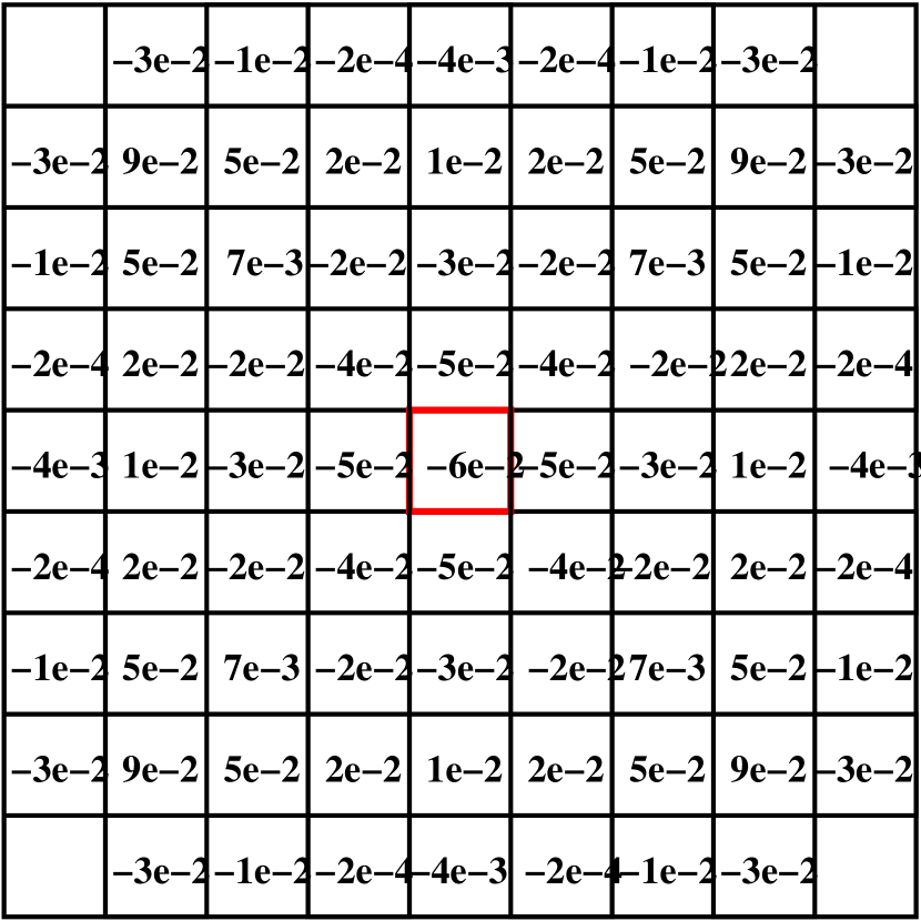
(a) Stencil for a regular cell using standard least squares.

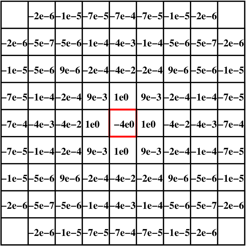
(b) Stencil for a regular cell using weighted least squares.

(c) Stencil for a cut cell using standard least squares.

(d) Stencil for a cut cell using weighted least squares.

Fig. 1: Fourth-order Laplacian stencil for the cell highlighted in red. Without weights, the stencil values do not decay with distance.

2.3 Order of Accuracy

In general, we cannot calculate the moments exactly. The geometry and the corresponding moments are constructed using the method in [20]. Let $M_{d,f}^{{\boldsymbol{p}}}({\boldsymbol{x}_{0}})$ denote the approximation to the exact moment $m_{d,f}^{{\boldsymbol{p}}}({\boldsymbol{x}_{0}})$, so that

$$M_{d,f}^{{\boldsymbol{p}}}({\boldsymbol{x}_{0}})=m_{d,f}^{{\boldsymbol{p}}}({\boldsymbol{x}_{0}})+O(h^{R}).$$

Recall that

$$\phi({\boldsymbol{x}})=\sum_{|{\boldsymbol{p}}|<P}c_{{\boldsymbol{p}}}({\boldsymbol{x}}-{\boldsymbol{x}_{0}})^{{\boldsymbol{p}}}+O(|{\boldsymbol{x}}-{\boldsymbol{x}_{0}}|^{P}).$$

In this subsection, we show that the truncation error for the kappa-weighted Laplacian operator is $O(h^{P-2})$ if $R=P+D-2$.

We assume that for face $f$, ${\boldsymbol{x}_{0}}$ is some point such that $|{\boldsymbol{x}}-{\boldsymbol{x}_{0}}|\leq Ch$ for all points ${\boldsymbol{x}}$ on the face. Then

$$\int_{\mathcal{A}_{f}}\nabla\phi\cdot{\boldsymbol{n}}d\mathcal{A} =\sum_{|{\boldsymbol{p}}|<P}c_{{\boldsymbol{p}}}\int_{\mathcal{A}_{f}}\nabla({\boldsymbol{x}}-{\boldsymbol{x}_{0}})^{{\boldsymbol{p}}}\cdot{\boldsymbol{n}}d\mathcal{A}+O(h^{P+D-2})$$

$$=\sum_{d=1}^{D}\sum_{|{\boldsymbol{p}}|<P}c_{{\boldsymbol{p}}}\int_{\mathcal{A}_{f}}p_{d}({\boldsymbol{x}}-{\boldsymbol{x}_{0}})^{{\boldsymbol{p}}-{\boldsymbol{e}^{d}}}n_{d}({\boldsymbol{x}})d\mathcal{A}+O(h^{P+D-2})$$

$$=\sum_{d=1}^{D}\sum_{|{\boldsymbol{p}}|<P}p_{d}c_{{\boldsymbol{p}}}m_{d,f}^{{\boldsymbol{p}}-{\boldsymbol{e}^{d}}}({\boldsymbol{x}_{0}})+O(h^{P+D-2})$$

$$=\sum_{d=1}^{D}\sum_{|{\boldsymbol{p}}|<P}p_{d}c_{{\boldsymbol{p}}}M_{d,f}^{{\boldsymbol{p}}-{\boldsymbol{e}^{d}}}({\boldsymbol{x}_{0}})+O(h^{R})+O(h^{P+D-2}).$$

We get

$$\frac{\kappa_{v}}{|\mathcal{V}_{v}|}\int_{\mathcal{V}_{v}}\nabla\cdot\nabla\phi\,d\mathcal{V} =\frac{1}{h^{D}}\sum_{f(v)}\int_{\mathcal{A}_{f}}\nabla\phi\cdot{\boldsymbol{n}}d\mathcal{A}$$

$$=\frac{1}{h^{D}}\sum_{f(v)}\sum_{d=1}^{D}\sum_{|{\boldsymbol{p}}|<P}p_{d}c_{{\boldsymbol{p}}}M_{d,f}^{{\boldsymbol{p}}-{\boldsymbol{e}^{d}}}({\boldsymbol{x}_{0}})+O(h^{R})+O(h^{P+D-2}).$$

At volumes $\mathcal{V}_{v}$ that are sufficiently far from the boundary (i.e. they only include regular volumes in their Laplacian stencils), the truncation error is $O(h^{P-1})$ if $R=P+D-1$. The $O(h^{P-2})$ term in the polynomial interpolation error cancels out because of symmetry in the flux stencils.

The truncation error is not the same for different choices of norms because of this disparity in the order of accuracy between volumes near the boundary and interior volumes. The error in the $L_{\infty}$ norm is $O(h^{P-2})$. In the $L_{1}$ norm, however, it is $O(h^{P-1})$. If $N=1/h$, then the number of volumes near the boundary is $O(N)$ whereas the number of interior volumes is $O(N^{2})$. So, the $L_{1}$ error looks like

$$\sum|e_{ij}|\Delta V\approx N^{2}(h^{P-1})(h^{2})+N(h^{P-2})(h^{2})=h^{P-1}.$$

In contrast, the solution error has the same order of accuracy in all the norms. Using potential theory arguments (see [12] for details), it can be shown that the error is $O(h^{P})$ near the boundary for Dirichlet boundary conditions and $O(h^{P-1})$ for Neumann boundary conditions. In the interior, the solution error is $O(h^{P-1})$. So, the order of accuracy in the solution is $Q$ if $P=Q+1$ and $R=Q+D$.

2.4 Neighbors and Weights

Recall, the polynomial interpolant $\psi$ is

$$\psi=\sum_{|{\boldsymbol{p}}|<P}c_{{\boldsymbol{p}}}({\boldsymbol{x}}-{\boldsymbol{x}_{0}})^{{\boldsymbol{p}}}.$$

In our method, we choose ${\boldsymbol{x}_{0}}$ to be the face center when $f$ is a grid-aligned face. If $f$ is an embedded boundary face, ${\boldsymbol{x}_{0}}$ is the center of the cell cut by $f$.

We take the neighbors of a volume $V$ to be the volumes in the physical domain that are $R_{n}$ cells away from $V$. We call $R_{n}$ the path radius. If a neighboring volume touchs a boundary face, then that boundary face is also regarded as a neighbor of $V$. The neighbors of a face $f$ are the neighbors of its adjacent volumes. See Figure 2.

For simplicity, our method uses one path radius for all volumes in the domain. To pin down the interpolant for a boundary face, we need a large path radius. In our results, we set $R_{n}=2$ for the second-order method, and $R_{n}=3$ for the fourth-order method.

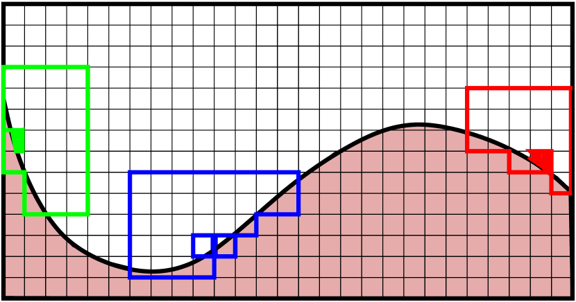
(a) Neighbors of a grid-aligned face (in blue) and two embedded boundary faces (whose corresponding cut cells are highlighted in red and green). In this diagram, the path radius $R_{n}$ is 3.

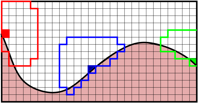
(b) Volumes involved in the Laplacian stencils for three volumes (highlighted in blue, green, and red).

Fig. 2: Neighbors used to construct stencils (flux stencils for faces and Laplacian stencils for volumes).

As explained at the end of Section 2.2.1, we want a weighting that emphasizes nearest neighbors, and gives little weight to far away neighbors. Our results were constructed with the weighting matrix $W$, with entries

$$W_{ii}=\begin{cases}1&\frac{|{\boldsymbol{x}}_{i}-{\boldsymbol{x}_{0}}|}{h}<\frac{1}{2}\\ (2\frac{|{\boldsymbol{x}}_{i}-{\boldsymbol{x}_{0}}|}{h})^{-5}&\frac{|{\boldsymbol{x}}_{i}-{\boldsymbol{x}_{0}}|}{h}\geq\frac{1}{2}\end{cases}.$$

If the $i$th row of $A$ (equation (9)) corresponds to a volume, then ${\boldsymbol{x}}_{i}$ is the cell center. If it corresponds to a grid-aligned boundary face, then ${\boldsymbol{x}}_{i}$ is the face center. Finally, if it corresponds to an embedded boundary face, then ${\boldsymbol{x}}_{i}$ is the cell center of the cut cell.

3 Results

In this section, we apply the method to solve Poisson’s equation on several different geometries, and demonstrate that the method achieves second and fourth order accuracy and produces a stable Laplacian operator.

3.1 Approximate Moments

The results presented in this paper were all obtained using $O(h^{6+D-1})$ accurate face moments and $O(h^{6+D})$ accurate volume moments. (Note that for $D=2$, the grid-aligned face moments are one-dimensional and are calculated exactly.)

3.2 Solver

We use the algebraic multigrid (AMG) method in the PETSc solver framework for our linear equation solves [4, 3, 5]. PETSc provides interfaces to several third party AMG solver and has a build in AMG solver, GAMG. We use a GMRES solver preconditioned with GAMG, which implements a smoothed aggregation AMG method [1]. To compute eigenvalues we use SLEPc, an extension of PETSc [11, 7]. The eigenvalues are found using Davidson methods [18].

3.3 Computing Convergence Rates

To compute convergence rates, we prescribe an exact solution and compare the computed quantities to the exact quantities. Convergence rates are calculated for the face fluxes, the operator truncation error, and the solution error. For a face $f$, the error in the face flux is

$$e^{\text{flux}}_{f}=\frac{1}{A_{f}}s_{f}^{T}\Phi-\frac{1}{A_{f}}\int_{f}\nabla\phi\cdot nd\mathcal{A},$$

where $s_{f}$ is the flux stencil (equation (11)) and $\Phi$ is defined in equation (10). Here, we have written $s_{f}$ instead of $s$ to highlight that $s$ depends on $f$. The flux error is computed for all of the faces, including boundary faces. The (kappa-weighted) truncation error for a volume $\mathcal{V}_{v}$ is

$$e^{\text{lapl}}_{v}=\frac{\kappa_{v}}{|\mathcal{V}_{v}|}\sum_{f(v)}s^{T}_{f(v)}\Phi-\frac{\kappa}{|\mathcal{V}_{v}|}\int_{\mathcal{V}_{v}}\Delta\phi d\mathcal{V}.$$

Finally, the solution error for $\mathcal{V}_{v}$ is the difference between the computed volume-average of $\phi$ and the exact volume-average.

The $L_{\infty}$ error is the maximum absolute error over the faces or the cells. For the flux, the $L_{1}$ error is defined as

$$e^{\text{flux}}_{L_{1}}=\frac{1}{\sum_{f}\alpha_{f}}\sum_{f}|e^{\text{flux}}_{f}|\alpha_{f}.$$

The $L_{1}$ truncation error is

$$e^{\text{lapl}}_{L_{1}}=\sum_{\mathcal{V}_{v}}|e^{\text{lapl}}_{v}||\mathcal{V}_{v}|.$$

Similarily for the solution error.

In each of 2D tests, the exact solution is

$$\phi(x,y)=\sin(2\pi(x-\sqrt{2}/2))\sin(2\pi(x-\sqrt{3}/2)).$$

The exact solution for the 3D example is given in Section 3.6.

3.4 Circle

Our first test geometry is the circle

$$(x-0.5)^{2}+(y-0.5)^{2}=0.25^{2}.$$

We apply the method to the region outside of this circle.

For this geometry, we simulate three cases:

1. 2nd order method with Dirichlet boundary conditions on the boundaries,

2. 4th order method with Dirichlet boundary conditions on the boundaries,

3. 4th order method with Dirichlet boundary conditions on the square and Neumann boundary conditions on the circle.

Figure 3 shows the solution error for test cases 2 and 3. Convergence rates are given in Table 1 for the three cases.

Figure 4(a) shows the spectra for the Laplacian operator in test cases 2 and 3. We have not weighted the operator by the volume fraction. In both cases the eigenvalues of the operator lie in the left half plane. There are a few eigenvalues with large negative real part. The eigenvectors corresponding to these eigenvalues are concentrated in the small cut cells. There is also a cluster of eigenvalues whose imaginary parts are relatively large. If this operator is combined with a temporal discretization like the trapezoidal rule to solve the heat equation, these eigenvalues would introduce oscillations in the solution; however, these oscillations are quickly damped out because the eigenvalues also have large negative real parts.

Without weights, the operator has large positive eigenvalues and is unstable (data not shown). The eigenvectors for the positive eigenvalues are supported on the small cells. The operator also has a pair of eigenvalues with significantly large imaginary parts, with eigenvectors that couple the smallest cells.

As a point of reference, we have plotted the spectrum for the second-order operator generated using the method in [19], (see Figure 5). This operator is weighted by the volume fraction. Like our fourth-order operator, this operator also has eigenvalues with non-negligible imaginary components.

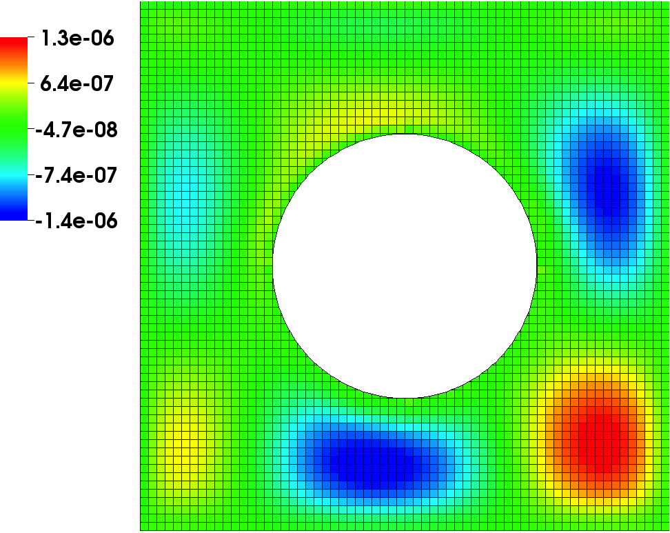
(a) Dirichlet boundary conditions on the circle.

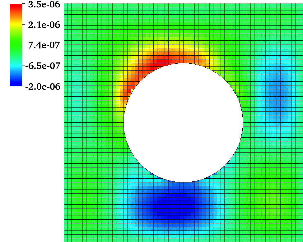
(b) Neumann boundary conditions on the circle.

Fig. 3: Solution error for fourth order method applied to area outside of circle with center $(0.5,0.5)$ and radius $0.25$. Dirichlet boundary conditions are prescribed on the square. The meshwidth of the Cartesian grid is $h=1/64$.

Test	$e_{32}$	Order	$e_{64}$	Order	$e_{128}$
2nd order, Dirichlet EB	5.01	1.03	2.44	1.72	7.43e-01
4th order, Dirichlet EB	9.36e-02	3.96	6.00e-03	2.62	9.72e-04
4th order, Neumann EB	5.30e-02	2.00	1.33e-02	2.83	1.87e-03

(a) $L_{\infty}$ convergence rates for $\kappa$-weighted truncation error.

Test	$e_{32}$	Order	$e_{64}$	Order	$e_{128}$
2nd order, Dirichlet EB	2.39e-01	1.91	6.39e-02	1.96	1.64e-02
4th order, Dirichlet EB	4.89e-03	3.97	3.11e-04	3.89	2.10e-05
4th order, Neumann EB	5.37e-03	3.87	3.68e-04	3.80	2.64e-05

(b) $L_{1}$ convergence rates for $\kappa$-weighted truncation error.

Test	$e_{32}$	Order	$e_{64}$	Order	$e_{128}$
2nd order, Dirichlet EB	1.36e-03	1.90	3.65e-04	1.92	9.64e-05
4th order, Dirichlet EB	2.56e-05	4.17	1.43e-06	3.86	9.80e-08
4th order, Neumann EB	5.24e-05	3.89	3.52e-06	3.94	2.29e-07

(c) $L_{\infty}$ convergence rates for solution error.

Test	$e_{32}$	Order	$e_{64}$	Order	$e_{128}$
2nd order, Dirichlet EB	4.06e-04	2.04	9.90e-05	1.97	2.52e-05
4th order, Dirichlet EB	5.70e-06	3.91	3.78e-07	3.91	2.52e-08
4th order, Neumann EB	1.07e-05	4.05	6.48e-07	3.96	4.16e-08

(d) $L_{1}$ convergence rates for solution error.

Table 1: Convergence rates for method applied to area outside of circle with center $(0.5,0.5)$ and radius $0.25$. $e_{N}$ is the error for a grid with meshwidth $h=1/N$. Dirichlet boundary conditions are prescribed on the square.

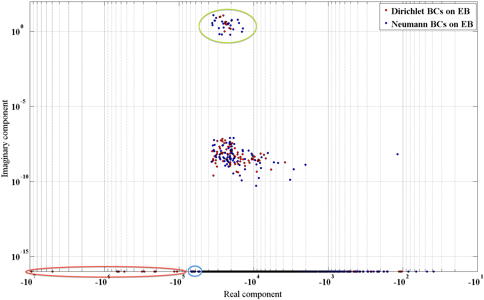
(a) Spectrum for fourth order method applied to domain outside of circle wih center $(0.5,0.5)$ and radius $0.25$. Dirichlet boundary conditions are prescribed on the square. The operator is not weighted by volume fraction. Only the eigenvalues with positive imaginary components are plotted because eigenvalues come in complex conjugate pairs. Independent of the circle boundary condition type, the operator has a few eigenvalues with large imaginary component (indicated by green circle). It also has large negative eigenvalues (indicated by the red circle for Dirchlet boundary conditions and the blue circle for Neumann boundary conditions) because small cells are present. The Cartesian grid is $64\times 64$.

Test Case	$\lambda^{*}$	$\lambda_{\text{max}}$	$\lambda_{\text{min}}$
$x_{0}=(0.5,0.5)$, $r=0.255$, Dirichlet BCs on EB	-3.6e4 + 28$i$	-106	-1.0e6
$x_{0}=(0.501,0.501)$, $r=0.25$, Dirichlet BCs on EB	-3.1e4 + 5.0$i$	-103	-2.5e6
$x_{0}=(0.5,0.5)$, $r=0.255$, Neumann BCs on EB	-3.0e4 + 24$i$	-39	-9.1e4
$x_{0}=(0.501,0.501)$, $r=0.25$, Neumann BCs on EB	-3.5e4 + 17$i$	-38	-1.3e5
$x_{0}=(0.51,0.5)$, $r=0.25$, Neumann BCs on EB	-2.0e4 + 10$i$	-38	-4.0e5

(b) Summary of spectra information for the fourth order method applied to the circle geometries. $x_{0}$ is the center of the circle, $r$ is the radius. The three columns are: the eigenvalue with the largest imaginary component ($\lambda^{*}$), the eigenvalue with the largest real component ($\lambda_{\text{max}}$), and the eigenvalue with the smallest real component ($\lambda_{\text{min}}$). Note that the eigenvalues come in complex conjugate pairs, and only the eigenvalue with a positive imaginary component is given in the first column.

Fig. 4:

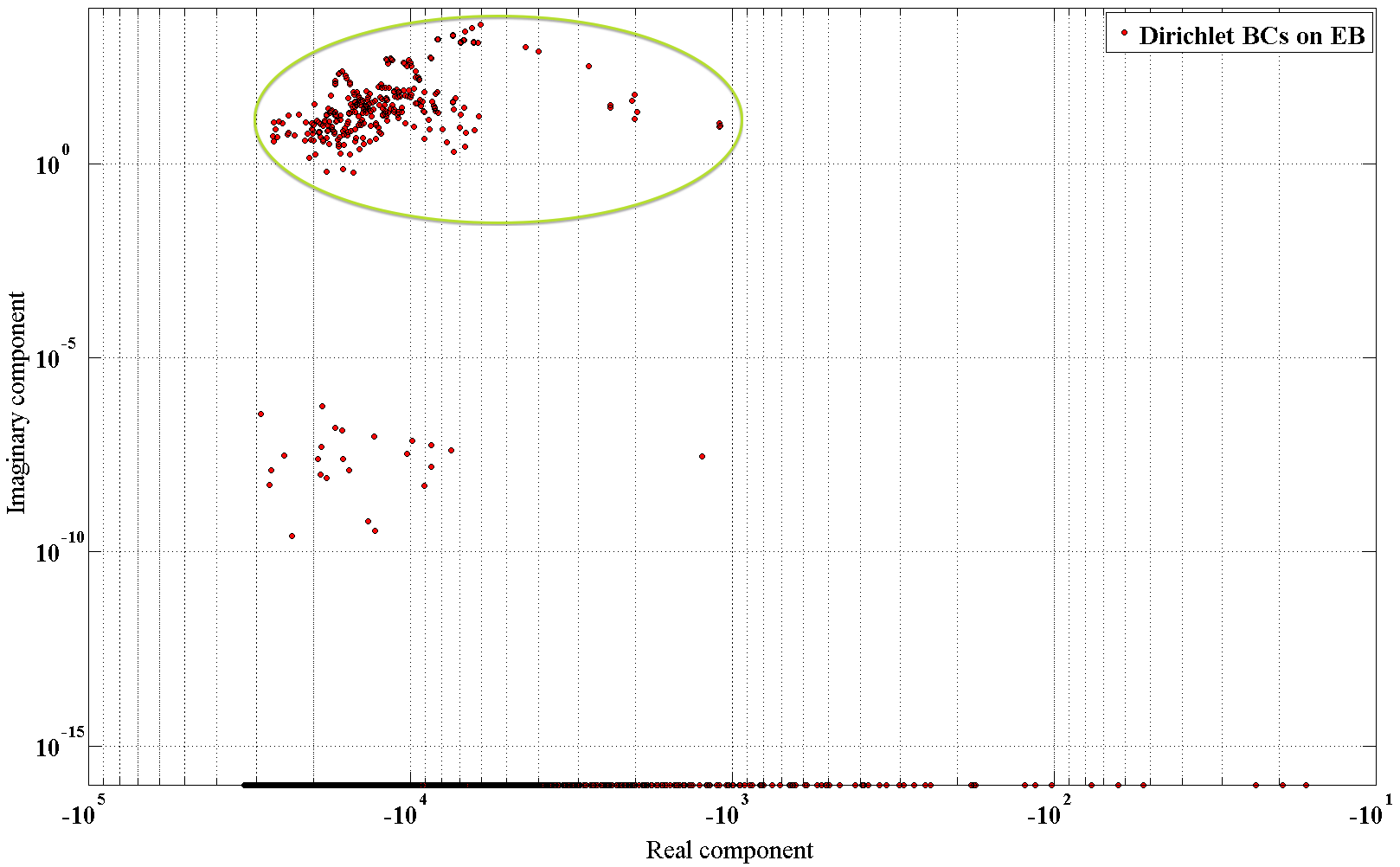
Fig. 5: Spectrum for operator generated using the method in [19]. The operator has been weighted by volume fraction. The domain is the region outside of the circle wih center $(0.5,0.5)$ and radius $0.25$. Dirichlet boundary conditions are prescribed on the boundaries. Like the operator for the weighted least squares method, this operator has a cluster of eigenvalues with non-negligible imaginary component (indicated by the green circle). The Cartesian grid is $64\times 64$.

3.4.1 Geometric Perturbations

Perturbations in the geometry can produce small cells. Our next set of tests demonstrates that the method is robust under small changes in the geometry. In particular, we perturb the radius and center of the circle in the last example, and apply the fourth order method to solve Poisson’s equation on the perturbed domains. Table 2 lists the smallest volume fractions for the original circle example and three perturbations of this circle on the three grids used in the study. Note that perturbing the circle’s center from $x_{0}=(0.5,0.5)$ to $x_{0}=(0.51,0.5)$ changes the smallest volume fraction by a magnitude!

Despite these differences in the geometry, the $\kappa$-weighted truncation error and solution error hardly change. Tables 3 and 4 display the convergence rates in the case of Dirichlet boundary conditions and Neumann boundary conditions on the embedded boundary, respectively.

The spectrum for each perturbation is similar to the spectrum in the previous example. The eigenvalues lie in the left half-plane for each of the perturbations. Also, there are a few eigenvalues with large negative real part corresponding to the small cells and a cluster of eigenvalues with non-negligible imaginary part. We summarize the main features of each spectrum in Figure 4.

Geometry	N=32	N=64	N=128
$x_{0}=(0.5,0.5)$, $r=0.25$	4.5e-3	1.0e-2	2.5e-4
$x_{0}=(0.5,0.5)$, $r=0.255$	1.7e-2	6.8e-3	9.5e-5
$x_{0}=(0.501,0.501)$, $r=0.25$	4.0e-4	1.6e-3	7.2e-6
$x_{0}=(0.51,0.5)$, $r=0.25$	3.6e-4	2.3e-4	4.5e-5

Table 2: Smallest volume fraction on a $N$x$N$ Cartesian grid for the domain outside of circle with center $x_{0}$ and radius $r$.

Test	$e_{32}$	Order	$e_{64}$	Order	$e_{128}$
$x_{0}=(0.5,0.5)$, $r=0.255$	7.24e-02	3.59	6.00e-03	3.10	7.01e-04
$x_{0}=(0.501,0.501)$, $r=0.25$	5.20e-02	3.12	6.00e-03	3.10	7.01e-04
$x_{0}=(0.51,0.5)$, $r=0.25$	7.41e-02	3.46	6.71e-03	2.39	1.28e-03

(a) $L_{\infty}$ convergence rates for $\kappa$-weighted truncation error

Test	$e_{32}$	Order	$e_{64}$	Order	$e_{128}$
$x_{0}=(0.5,0.5)$, $r=0.255$	4.93e-03	3.92	3.26e-04	3.91	2.17e-05
$x_{0}=(0.501,0.501)$, $r=0.25$	4.87e-03	3.95	3.14e-04	3.87	2.14e-05
$x_{0}=(0.51,0.5)$, $r=0.25$	5.06e-03	3.98	3.21e-04	3.91	2.14e-05

(b) $L_{1}$ convergence rates for $\kappa$-weighted truncation error

Test	$e_{32}$	Order	$e_{64}$	Order	$e_{128}$
$x_{0}=(0.5,0.5)$, $r=0.255$	2.01e-05	3.85	1.40e-06	3.88	9.48e-08
$x_{0}=(0.501,0.501)$, $r=0.25$	3.38e-05	4.55	1.45e-06	3.88	9.84e-08
$x_{0}=(0.51,0.5)$, $r=0.25$	3.02e-05	3.34	2.97e-06	4.91	9.88e-08

(c) $L_{\infty}$ convergence rates for solution error

Test	$e_{32}$	Order	$e_{64}$	Order	$e_{128}$
$(x_{0},y_{0})=(0.5,0.5)$, $r=0.255$	5.56e-06	3.90	3.73e-07	3.92	2.47e-08
$(x_{0},y_{0})=(0.501,0.501)$, $r=0.25$	6.06e-06	4.00	3.79e-07	3.91	2.51e-08
$(x_{0},y_{0})=(0.51,0.5)$, $r=0.25$	5.94e-06	3.93	3.90e-07	3.96	2.50e-08

(d) $L_{1}$ convergence rates for solution error

Table 3: Convergence rates for 4th order method applied to domain outside of the circle $(x-x_{0})^{2}+(y-y_{0})^{2}=r^{2}$. Dirichlet boundary conditions are prescribed on the boundaries.

Test	$e_{32}$	Order	$e_{64}$	Order	$e_{128}$
$x_{0}=(0.5,0.5)$, $r=0.255$	5.19e-02	2.29	1.06e-02	2.48	1.90e-03
$x_{0}=(0.501,0.501)$, $r=0.25$	5.17e-02	2.03	1.27e-02	2.69	1.96e-03
$x_{0}=(0.51,0.5)$, $r=0.25$	5.53e-02	2.09	1.30e-02	2.63	2.10e-03

(a) $L_{\infty}$ convergence rates for $\kappa$-weighted truncation error

Test	$e_{32}$	Order	$e_{64}$	Order	$e_{128}$
$x_{0}=(0.5,0.5)$, $r=0.255$	5.41e-03	3.77	3.95e-04	3.90	2.64e-05
$x_{0}=(0.501,0.501)$, $r=0.25$	5.42e-03	3.86	3.72e-04	3.85	2.581e-05
$x_{0}=(0.51,0.5)$, $r=0.25$	5.40e-03	3.82	3.83e-04	3.91	2.542e-05

(b) $L_{1}$ convergence rates for $\kappa$-weighted truncation error

Test	$e_{32}$	Order	$e_{64}$	Order	$e_{128}$
$x_{0}=(0.5,0.5)$, $r=0.255$	5.41e-05	3.95	3.49e-06	3.94	2.27e-07
$x_{0}=(0.501,0.501)$, $r=0.25$	5.32e-05	3.91	3.53e-06	3.95	2.29e-07
$x_{0}=(0.51,0.5)$, $r=0.25$	5.52e-05	3.95	3.58e-06	3.94	2.33e-07

(c) $L_{\infty}$ convergence rates for solution error

Test	$e_{32}$	Order	$e_{64}$	Order	$e_{128}$
$x_{0}=(0.5,0.5)$, $r=0.255$	1.09e-05	4.08	6.45e-07	3.97	4.12e-08
$x_{0}=(0.501,0.501)$, $r=0.25$	1.08e-05	4.06	6.48e-07	3.96	4.17e-08
$x_{0}=(0.51,0.5)$, $r=0.25$	1.11e-05	4.08	6.55e-07	3.96	4.21e-08

(d) $L_{1}$ convergence rates for solution error

Table 4: Convergence rates for 4th order method applied to domain outside of the circle $(x-x_{0})^{2}+(y-y_{0})^{2}=r^{2}$. Dirichlet boundary conditions are prescribed on the square, and Neumann boundary conditions are prescribed on the circle.

3.5 Other Geometries

In the next few sections, we apply the fourth order method on different geometries. In each case, the operator spectrum looks similar to the circle example: there are a few eigenvalues with large negative part that correspond to small cells and a cluster of eigenvalues with non-negligible imaginary part. As a result, we summarize the main features of the spectra in Table 7.

3.5.1 Trignometric Curve

Our next domain is the region underneath the curve

$$y=0.25+\frac{\sqrt{2}}{2}(1-\cos(2\pi x)).$$ (13)

We apply the fourth order method to solve Poisson’s equation on this geometry. Dirichlet boundary conditions are prescribed on the boundaries. Figure 6 shows the solution error on the grid with meshwidth $h=1/128$, and Table 5 lists the convergence rates. It is clear that the method converges at fourth order for this example.

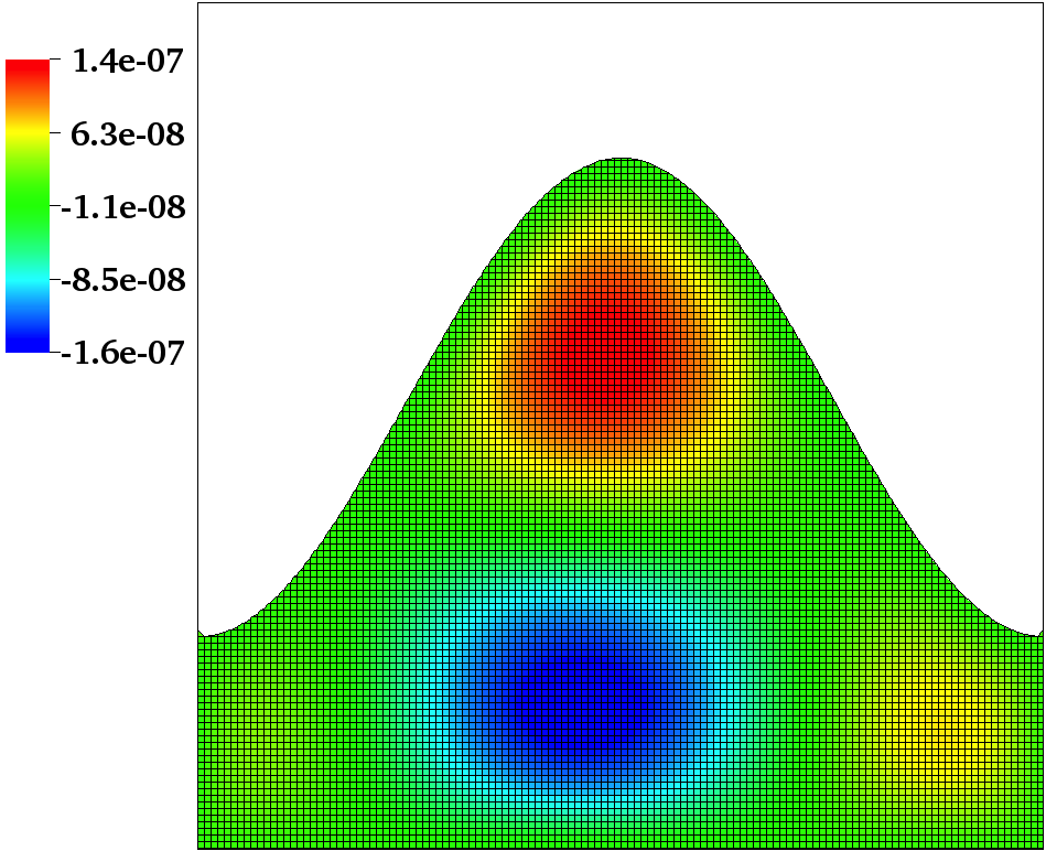
Fig. 6: Solution error from fourth order method applied to area underneath the curve $y=0.25+\frac{\sqrt{2}}{2}(1-\cos(2\pi x))$. Dirichlet boundary conditions are prescribed on the boundaries. The Cartesian grid is $128\times 128$.

Test	$e_{32}$	Order	$e_{64}$	Order	$e_{128}$
$\kappa$-weighted truncation error, $L_{\infty}$	7.82e-02	3.38	7.53e-03	3.06	9.03e-04
$\kappa$-weighted truncation error, $L_{1}$	3.99e-03	3.75	2.97e-04	3.86	2.05e-05
Solution error, $L_{\infty}$	4.03e-05	3.99	2.53e-06	4.00	1.58e-07
Solution error, $L_{1}$	1.10e-05	3.91	7.32e-0	3.93	4.82e-08

Table 5: Convergence rates for fourth order method applied to area underneath the curve $y=0.25+\frac{\sqrt{2}}{2}(1-\cos(2\pi x))$. Dirichlet boundary conditions are prescribed on the boundaries.

3.5.2 Four circles

Next, we consider the domain outside of the four circles with centers $(0.25,0.25)$, $(0.75,0.25)$, $(0.25,0.75)$, $(0.75,0.75)$ and all with radius $0.215$. We apply the fourth order method; Dirichlet boundary conditions are prescribed on the boundaries. Figure 7 shows the solution error on the grid with meshwidth $1/128$.

Unlike the previous examples, we simulate this example on grids with $N=$64, 128, and 256 because the $N=32$ is too coarse to compute a fourth order flux. On the $64x64$ grid, each of the circles is only $3$ grid cells away from the square boundary. Thus, a face close to the boundary has the minimum information to construct a fourth order flux: 3 cells, 1 embedded boundary face, and 1 domain boundary face. Despite this limited information, the $\kappa$-weighted truncation error and solution error converge at fourth order. Also, the operator is stable (see Table 7).

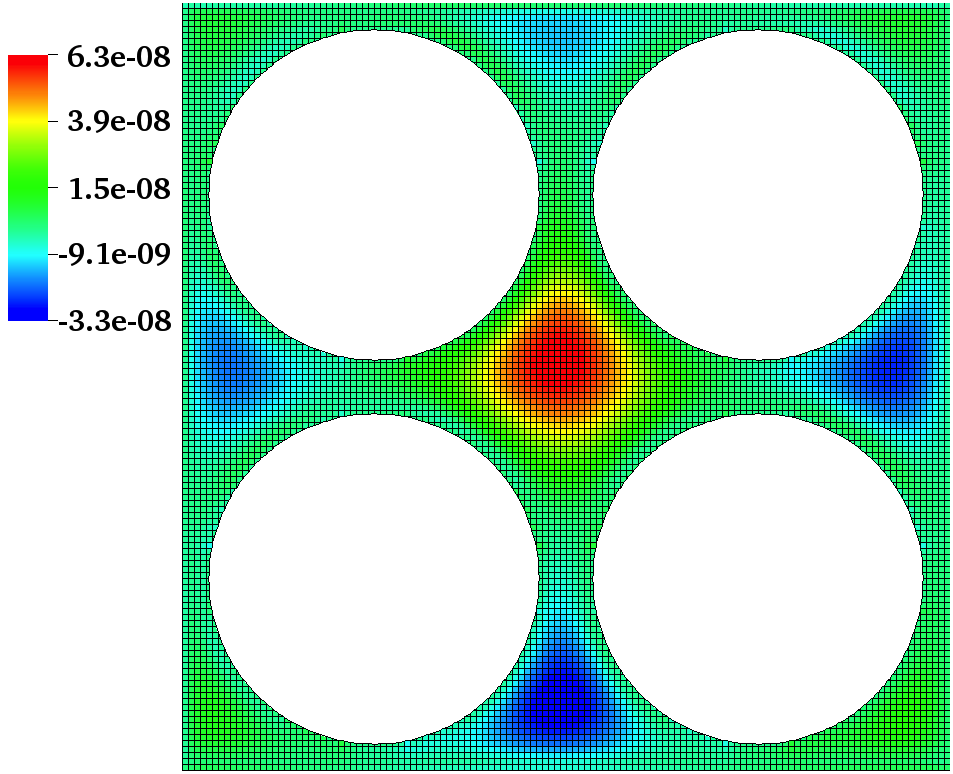
Fig. 7: Solution error from 4th order applied to the area outside of four circles that are close to the square boundary. Dirichlet boundary conditions are prescribed on the boundaries. The Cartesian grid is $128\times 128$.

Test	$e_{64}$	Order	$e_{128}$	Order	$e_{256}$
Truncation error with kappa, $L_{\infty}$	3.45e-02	5.24	9.13e-04	3.19	1.00e-04
Truncation error with kappa, $L_{1}$	1.12e-03	4.61	4.62e-05	3.90	3.10e-06
Solution error, $L_{\infty}$	1.04e-06	4.04	6.30e-08	3.94	4.11e-09
Solution error, $L_{1}$	1.73e-07	4.12	9.98e-09	3.88	6.77e-10

Table 6: Convergence rates for fourth order method where the domain is the outside of four circles that are close to the square boundary.

Test Case	$\lambda^{*}$	$\lambda_{\text{max}}$	$\lambda_{\text{min}}$
$x_{0}=(0.5,0.5)$, $r=0.25$, Dirichlet BCs on EB	-2.5e4 + 11$i$	-104	-9.5e6
$x_{0}=(0.5,0.5)$, $r=0.255$, Dirichlet BCs on EB	-3.6e4 + 28$i$	-106	-1.0e6
$x_{0}=(0.501,0.501)$, $r=0.25$, Dirichlet BCs on EB	-3.1e4 + 5.0$i$	-103	-2.5e6
$x_{0}=(0.5,0.5)$, $r=0.25$, Neumann BCs on EB	-3.5e4 + 12$i$	-38	-6.9e4
$x_{0}=(0.5,0.5)$, $r=0.255$, Neumann BCs on EB	-3.0e4 + 24$i$	-39	-9.1e4
$x_{0}=(0.501,0.501)$, $r=0.25$, Neumann BCs on EB	-3.5e4 + 17$i$	-38	-1.3e5
$x_{0}=(0.51,0.5)$, $r=0.25$, Neumann BCs on EB	-2.0e4 + 10$i$	-38	-4.0e5
Other geometries
Four circles, Dirichlet BCs on EB	-4.4e4 + 1.6e3$i$	-240	-6.4e5
Sine curve, Dirichlet BCs on EB	-3.3e4 + 600$i$	-51	-1.8e6

Table 7: Summary of spectra information for the 4th order method applied to various geometries. The three columns are: the eigenvalue with the largest imaginary component ($\lambda^{*}$), the eigenvalue with the largest real component ($\lambda_{\text{max}}$), and the eigenvalue with the smallest real component ($\lambda_{\text{min}}$). Note that the eigenvalues come in complex conjugate pairs, and only the eigenvalue with a positive imaginary component is given in the first column. The meshwidth of the Cartesian grid is $1/64$. Dirichlet boundary conditions are prescribed on the square boundary.

3.6 Sphere

In this section, we apply a fourth order method to solve Poisson’s equation on the inside of a sphere, with center $(0.5,0.5,0.5)$ and radius 0.45. The exact solution for this test problem is

$$\phi(x,y,z)=\sin(2\pi(x-x_{0}))\sin(2\pi(y-y_{0}))\sin(2\pi(z-z_{0})),$$ (14)

where $x_{0}=\sqrt{2}/2$, $y_{0}=\sqrt{3}/2$, and $z_{0}=0.54321$. Table 8 shows the solution error convergence rates. It is clear that the method is fourth order. Figure 8 shows the solution error on a grid with meshwidth $h=1/128$.

Norm	$e_{32}$	Order	$e_{64}$
$L_{\infty}$	9.16e-05	3.87	6.27e-06
$L_{1}$	1.38e-05	3.81	9.81e-07
$L_{2}$	2.17e-05	3.81	1.54e-06

Table 8: Solution error convergence rates in the $L_{\infty}$, $L_{1}$, and $L_{2}$ norms for 4th order method applied to inside of sphere with center $(0.5,0.5,0.5)$ and radius $0.45$.

Fig. 8: Solution error for 4th order method applied to inside of sphere with center $(0.5,0.5,0.5)$ and radius $0.45$. Each image shows three cross-sections through the center of the sphere. The triad next to each image shows the orientation of the sphere in the image.

4 Conclusions

We have presented an algorithm to generate higher-order conservative finite volume discretizations for Poisson’s equation on cut cell grids. The Poisson operator is written in terms of face fluxes, which we approximate using a polynomial interpolant. The key to the method is to use weighted least squares to generate stable stencils. In particular, the linear system for the face flux stencil is underdetermined, and we can use weights to pick a stable stencil from the space of solutions.

By applying the method to a variety of geometries, we have demonstrated that the method achieves second and fourth order accuracy. In each of these examples, we have also shown that the discrete Laplacian operator is stable; that is, it has strictly negative eigenvalues.

We are currently studying the effect of different weighting functions on the operator spectrum for a future theory paper. We are also looking into how other choices, like neighbor selection and centering of the interpolant, modify the spectrum. Our current method produces a Laplacian operator with eigenvalues that depend on the inverse of the smallest volume fractions. The operator spectrum also contains a small cluster of eigenvalues with non-negligible imaginary components. We hope to alleviate both problems in the future. Finally, we plan to study the effect of using standard regular stencils in the interior for the theory paper.

The method described in this paper is applicable to other problems in div-flux form. For example, we are working on a fourth-order method for advection-diffusion. For this problem, we are using an upwind weighting system. Another application for the future is the variable coefficient Poisson’s equations for smoothly varying coefficients.

References

- [1] M. F. Adams. Algebraic multigrid methods for constrained linear systems with applications to contact problems in solid mechanics. Numerical Linear Algebra with Applications, 11(2-3):141–153, 2004.
- [2] M. J. Aftosmis, M. J. Berger, and J. S. Saltzman. Robust and efficient cartesian mesh generation for component-base geometry. AIAA Journal, 36(6):952–960, June 1998.
- [3] S. Balay, S. Abhyankar, M. F. Adams, J. Brown, P. Brune, K. Buschelman, V. Eijkhout, W. D. Gropp, D. Kaushik, M. G. Knepley, L. C. McInnes, K. Rupp, B. F. Smith, and H. Zhang. PETSc users manual. Technical Report ANL-95/11 - Revision 3.5, Argonne National Laboratory, 2014.
- [4] S. Balay, S. Abhyankar, M. F. Adams, J. Brown, P. Brune, K. Buschelman, V. Eijkhout, W. D. Gropp, D. Kaushik, M. G. Knepley, L. C. McInnes, K. Rupp, B. F. Smith, and H. Zhang. PETSc Web page. http://www.mcs.anl.gov/petsc, 2014.
- [5] S. Balay, W. D. Gropp, L. C. McInnes, and B. F. Smith. Efficient management of parallelism in object oriented numerical software libraries. In E. Arge, A. M. Bruaset, and H. P. Langtangen, editors, Modern Software Tools in Scientific Computing, pages 163–202. Birkhäuser Press, 1997.
- [6] S. Brenner and R. Scott. The Mathematical Theory of Finite Element Methods. Springer, New York, 2007.
- [7] C. Campos, J. E. Roman, E. Romero, and A. Tomas. SLEPc users manual. Technical Report DSIC-II/24/02 - Revision 3.3, D. Sistemes Informàtics i Computació, Universitat Politècnica de València, 2012.
- [8] H. Cheng, L. Greengard, and V. Rokhlin. A fast adaptive multipole algorithm in three dimensions. JCP, 155:468–496, 1999.
- [9] F. Gibou and R. Fedkiw. A fourth order accurate discretization for the laplace and heat equations on arbitrary domains, with applications to the stefan problem. J. Comput. Phys., 202:577–601, 2005.
- [10] L. Greengard and J.-Y. Lee. A direct adaptive poisson solver of arbitrary order accuracy. J. Comput. Phys., 125:415–424, 1996.
- [11] V. Hernandez, J. E. Roman, and V. Vidal. SLEPc: Scalable Library for Eigenvalue Problem Computations. Lecture Notes in Computer Science, 2565:377–391, 2003.
- [12] H. Johansen and P. Colella. A cartesian grid embedded boundary method for poisson’s equation on irregular domains. J. Comput. Phys., 147(1):60–85, 1998.
- [13] H. S. Johansen and P. Colella. A Cartesian grid embedded boundary method for Poisson’s equation on irregular domains. J. Comput. Phys., 147(2):60–85, December 1998.
- [14] R. LeVeque and Z. Ling. The immersed interface method for elliptic equations with discontinuous coefficients and singular sources. SIAM Journal of Numerical Analysis, 31(4):1019–1044, 1994.
- [15] R. J. LeVeque. Numerical Methods for Conservation Laws. Birkhauser-Verlag, Basel, Boston, Berlin, 1990.
- [16] A. McKenney, L. Greengard, and A. Mayo. A fast poisson solver for complex geometries. J. Comput. Phys., 118:348–355, 1995.
- [17] S. Pirzadeh. Advanced unstructured grid generation for complex aerodynamic applications. AIAA Journal, 48(5):904–915, 2010.
- [18] E. Romero and J. E. Roman. A parallel implementation of Davidson methods for large-scale eigenvalue problems in SLEPc. ACM Trans. Math. Software, 40(2):13:1–13:29, 2014.
- [19] P. Schwartz, M. Barad, P. Colella, and T. Ligocki. A Cartesian grid embedded boundary method for the heat equation and Poisson’s equation in three dimensions. Journal of Computational Physics, 211(2):531–550, Jan. 2006.
- [20] P. Schwartz, J. Percelay, T. Ligocki, H. Johansen, D. T. Graves, D. Devendran, P. Colella, and E. Ateljevich. High accuracy embedded boundary grid generation using the divergence theorem. Accepted by CAMCoS, 2014.