Tensor renormalization group study of the 2d O(3) model
Abstract:
We present our progress on a study of the model in two-dimensions using the Tensor Renormalization Group method. We first construct the theory in terms of tensors, and show how to construct -point correlation functions. We then give results for thermodynamic quantities at finite and infinite volume, as well as 2-point correlation function data. We discuss some of the advantages and challenges of tensor renormalization and future directions in which to work.
1 The Model & Tensor Renormalization
In the following we consider the non-linear sigma model with Hamiltonian
| (1) |
where is a three-component vector, and a sum over nearest-neighbor pairs on a two-dimensional square lattice. The partition function is
| (2) |
The sum is over spin configurations on a two-dimensional lattice, and is the unit spherical area element. This model is important for a number of reasons. Firstly, it has a non-Abelian global symmetry. Second, the model has no spontaneous symmetry breaking (i.e. for all ), unlike the Ising model in two dimensions. Thirdly, this model is known to be asymptotically free for large . Lastly, the model also possesses instantons which are labeled by an integer topological index.
The Tensor Renormalization Group (TRG) [1] is a renormalization group method developed for classical statistical models. TRG consists of reformulating a classical partition function in terms of local tensors. The techniques used here are similar to [2], which hinge on using Higher Order Singular Value Decomposition (HOSVD), giving the renormalization group technique the name Higher Order Tensor Renormalization Group (HOTRG). The methodology is as follows. First one must form the initial tensor, or devise a tensor formulation for one’s model. Second, one performs a blocking step. A blocking step includes contracting two tensors together, then using the HOSVD to pick out the most relevant directions in renormalization group product space. Once we pick out the relevant directions in renormalization group space, we project out those states to form a new tensor. This process is illustrated in Figure 1.
1. 2.
2. 3.
3.
The tensor formulation allows one to decouple the lattice at the location of the local constraint, in our case, the sites of the lattice. The lattice is then rebuilt by piecing these tensors together geometrically in the shape of the lattice. The idea of contracting the tensors to build up a lattice is shown in Figure 2.

2 Tensor Formulation for
A simple approach to formulating the model in terms of tensors is through harmonic analysis. has two quantum numbers: and . However the expansion coefficients, when expanding in terms of Legendre polynomials, only depend on . To proceed we expand the Boltzmann weight in terms of Legendre polynomials
| (3) |
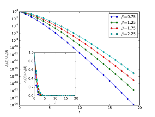
The relative size of the coefficients can be seen in Figure 3. Now
| (4) |
This allows us to factorize the initial contribution from the links. With the angular dependence decoupled, angular integration can now take place, and the theory can be written in terms of integer-valued fields , and .
The spherical harmonics are associated with pairs of sites, or links. Since there are four impinging links per site on the lattice, the angular integration is built out of four spherical harmonics. This integral is responsible for the constraint at a site and has the form
| (5) | |||
| (6) |
This constraint enforces the triangle in-equalities between pairs of external legs of the tensor and intermediate angular momentum quantum numbers. The intermediate sum over and picks out irreducible representations of the angular momenta. A picture of how one might interpret the tensor is shown in Figure 4. The tensor can be written down explicitly as
| (7) |
with the constraint from before, and the location on the lattice. This is in contrast with the Abelian constraint, which simply demands a conservation of the integer-valued fields associated with the links at their common site.

From this tensor the entire partition function and the free energy can be built up and thermodynamical quantities calculated.
3 -point Correlations
-point correlations can be realized on the lattice by inserting spin vectors at particular sites. This comes from the typical expression for correlation functions
| (8) |
These additional spin vectors lead to a modified constraint at each site of insertion. This comes about by expanding the Boltzmann weight as usual, however there are additional degrees of freedom to integrate due to the modified integrand. The integrand can be made more suitable for integration by using the spherical basis,
| (9) |
as a representation for the spin vectors. The angular integral that needs to be preformed at each site of insertion now has the form
| (10) | |||
| (11) | |||
| (12) |
This leads to a tensor whose elements are shifted, or an “impure” tensor.

Average values are computed by contracting these impure tensors with pure tensors using the same algorithmics. The number of impure tensors used during the contraction pattern (and when applicable, their relative separation) determines which -point function one is computing, and what modes one is considering. For -point functions it is necessary to have a source and a sink, i.e. two impure tensors in the lattice (in the absence of a magnetic field). A picture of the insertion of a spin into the lattice using an impure tensor is shown in Figure 5.
4 Results
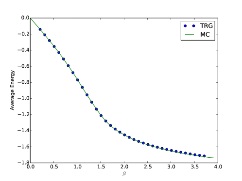
Here we report some of the results obtained during this study. While it has been shown that TRG is able to reproduce numerical data comparable to Monte Carlo simulations for the model [3], it was nevertheless important to cross check observables for since it has not been done using TRG. In Figure 6 we show a comparison between Monte Carlo and TRG for the average energy at finite volume.
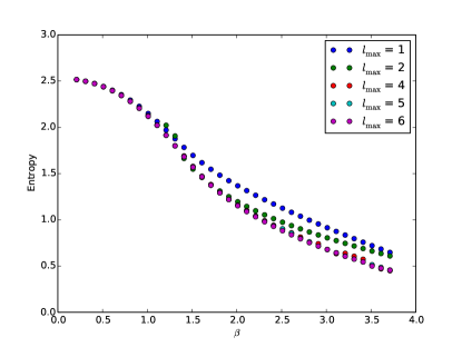
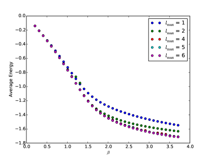
It was then best to use TRG to explore regions where Monte Carlo has difficulty, namely, the infinite volume limit. In Figure 7 we see results for the infinite volume limit for average energy and entropy. The number of states kept during iterations is given in terms of the total angular momentum number . For the number of states, , in terms of is given by .
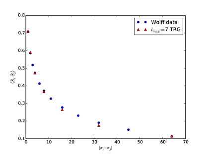
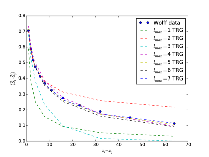
Finally, in Figure 8 we see data from TRG for the 2-point correlation function and the comparison to Table 2 in Ref. [4].
5 Conclusion and Future Work
Tensor renormalization is a powerful method in 2D for extracting infinite volume thermodynamics. However, it appears to give inaccurate results for -point correlation functions so far. TRG appears insensitive to the sign problem [5] and computing in the infinite volume limit is as easy as computing at finite volume, since if one can compute a single block-spin, one can compute any number of them. It’s also possible to formulate many popular models in terms of tensors, and a tensor formulation comes with a convenient graphical representation [6].
Another point of interest is the fact that particular tensor elements in the tensor formulation are negative. It is unclear at this point if this formulation has negative weights for configurations. Alternatively, there are reformulations of the model where all the weights are positive definite [7]. It would be interesting to attempt other tensor formulations where one can be sure that the weights are positive.
Understanding the systematic improvement of TRG and how the number of states kept during iterations improves accuracy is also a point of interest. While ideally if one could keep all the configurations of the system the results would be exact, one can only keep a finite amount, and it becomes important to understand the optimal way to keep higher numbers of states. In terms of scaling, TRG scales as in CPU time in two-dimensions, and the memory scales as . Parallelization of tensor contractions could help the scaling.
Acknowledgements
This research was supported in part by the Department of Energy under Award Number DOE grant DE-SC0010114. In addition, this research used resources of the Argonne Leadership Computing Facility, which is a DOE Office of Science User Facility supported under Contract DE-AC02-06CH11357.
References
- [1] M. Levin and C. P. Nave, “Tensor renormalization group approach to two-dimensional classical lattice models,” Phys. Rev. Lett., vol. 99, p. 120601, Sep 2007.
- [2] Z. Y. Xie, J. Chen, M. P. Qin, J. W. Zhu, L. P. Yang, and T. Xiang, “Coarse-graining renormalization by higher-order singular value decomposition,” Phys. Rev. B 86, 045139, 2012.
- [3] J. F. Yu, Z. Y. Xie, Y. Meurice, Y. Liu, A. Denbleyker, H. Zou, M. P. Qin, J. Chen, and T. Xiang, “Tensor renormalization group study of classical XY model on the square lattice,” Phys. Rev. E 89, 013308, 2014.
- [4] U. Wolff, “Asymptotic freedom and mass generation in the O(3) nonlinear -model,” Nucl. Phys. B 334, 581, 1990.
- [5] A. Denbleyker, Y. Liu, Y. Meurice, M. P. Qin, T. Xiang, Z. Y. Xie, J. F. Yu, and H. Zou, “Controlling sign problems in spin models using tensor renormalization,” Phys. Rev. D 89, 016008, 2014.
- [6] Y. Liu, Y. Meurice, M. P. Qin, J. Unmuth-Yockey, T. Xiang, Z. Y. Xie, J. F. Yu, and H. Zou, “Exact blocking formulas for spin and gauge models,” Phys. Rev. D, vol. 88, p. 056005, Sep 2013.
- [7] U. Wolff, “Simulating the all-order strong coupling expansion III: O(N) sigma/loop models,” Nucl. Phys. B 824, 254, 2010.