Grouped variable importance with random forests and application to multiple functional data analysis

Abstract

The selection of grouped variables using the random forest algorithm is considered. First a new importance measure adapted for groups of variables is proposed. Theoretical insights into this criterion are given for additive regression models. Second, an original method for selecting functional variables based on the grouped variable importance measure is developed. Using a wavelet basis, it is proposed to regroup all of the wavelet coefficients for a given functional variable and use a wrapper selection algorithm with these groups. Various other groupings which take advantage of the frequency and time localization of the wavelet basis are proposed. An extensive simulation study is performed to illustrate the use of the grouped importance measure in this context. The method is applied to a real life problem coming from aviation safety.

1 Introduction

In the high dimensional setting, identification of the most relevant variables has been the subject of much research during the last two decades [Guyon and Elisseeff, 2003]. For linear regression, the lasso method [Tibshirani, 1996] is widely used. Many variable selection procedures have also been proposed for non linear methods. In the context of random forests [Breiman, 2001], it has been shown that the permutation importance measure is an efficient tool for selecting variables [Díaz-Uriarte and Alvarez de Andrés, 2006, Genuer et al., 2010, Gregorutti et al., 2014].

In many situations such as medical studies and genetics, groups of variables can be clearly identified and it is of interest to select groups of variables rather than to select them individually [He and Yu, 2010]. Indeed, interpretation of the model may be improved along with the prediction accuracy by grouping the variables according to a priori knowledge about the data. Furthermore, grouping variables can be seen as a solution to stabilize variable selection methods. In the linear setting, and more particularly for linear regression, the group lasso has been developed to deal with groups of variables, see for instance Yuan and Lin [2006a]. Group variable selection has also been proposed for kernel methods [Zhang et al., 2008] and neural networks [Chakraborty and Pal, 2008]. As far as we know, this problem has not been studied for the random forest algorithm introduced by Breiman [2001]. In this paper, we adapt the permutation importance measure for groups of variables in order to select groups of variables in the context of random forests.

The first contribution of this paper is a theoretical analysis of the grouped variable importance measure. Generally speaking, the grouped variable importance does not reduce to the sum of the individual importances and may even be quite unrelated to it. However, in more specific models such as additive regression ones, we derive exact decompositions of the grouped variable importance measure.

The second contribution of this work is an original method for selecting functional variables based on the grouped variable importance measure. Functional Data Analysis (FDA) is a field in statistics that analyzes data indexed by a continuum. In our case, we consider data providing information about curves varying over time [Ramsay and Silverman, 2005, Ferraty and Vieu, 2006, Ferraty, 2011]. One standard approach in FDA consists in projecting the functional variables onto a finite dimensional space spanned by a functional basis. Classical bases in this context are splines, Fourier, wavelets or Karhunen-Loève expansions, for instance. Most of the papers about regression and classification methods for functional data consider only one functional predictor; references include Cardot et al. [1999, 2003], Rossi et al. [2006], Cai and Hall [2006] for linear regression methods, Amato et al. [2006], Araki et al. [2009] for logistic regression methods, Górecki and Smaga [2015] for ANOVA problem, Biau et al. [2005], Fromont and Tuleau [2006] for $k$-NN algorithms and Rossi and Villa [2006, 2008] for SVM classification. The multiple FDA problem, where $p$ functional variables are observed, has been less studied. Recently, Matsui and Konishi [2011] and Fan and James [2013] have proposed solutions to the linear regression problem with lasso-like penalties. The logistic regression case has been studied by Matsui [2014]. Classification based on several functional variables has also been considered using the CART algorithm [Poggi and Tuleau, 2006] and SVM [Yang et al., 2005, Yoon and Shahabi, 2006].

We propose a new approach for multiple FDA using random forests and the grouped variable importance measure. Indeed, various groups of basis coefficients can be proposed for a given functional decomposition. For instance, one can choose to regroup all coefficients of a given functional variable. In this case, the selection of a group of coefficients corresponds to the selection of a functional variable. Various other groupings are proposed for wavelet decompositions. For a given family of groups, we adapt the recursive feature elimination algorithm [Guyon et al., 2002] which is particularly efficient when predictors are strongly correlated [Gregorutti et al., 2014]. In the context of random forests, this backward-like selection algorithm is guided by the grouped variable importance. Note that by regrouping the coefficients, the computational cost of the algorithm is drastically reduced compared to a backward strategy that would eliminate only one coefficient at each step.

An extensive simulation study illustrates the application of the grouped importance measure for FDA. The method is then applied to a real life problem coming from aviation safety. The aim of this study is to explain and predict landing distances. We select the most relevant flight parameters regarding the risk of long landings, which is a major issue for airlines.

The group permutation importance measure is introduced in Section 2. Section 3 deals with multiple FDA using random forests and the grouped variable importance measure. The application to flight data analysis is presented in Section 4. Note that additional experiments about the grouped variable importance are given in B. In order to speed up the algorithm, the dimension of the data can be reduced in a preprocessing step. In C, we propose a modified version of a well-known shrinkage method [Donoho and Johnstone, 1994] that simultaneously shrinks to zero the coefficients of the observed curves of a functional variable.

2 The grouped variable importance measure

Let $Y$ be a random variable in $\mathbb{R}$ and $\mathbf{X}^{\top}=(X_{1},\dots,X_{p})$ a random vector in $\mathbb{R}^{p}$. We denote by $f(\mathbf{x})=\mathbb{E}[Y|\mathbf{X}=\mathbf{x}]$ the regression function. Let $\operatorname*{Var}(\mathbf{X})$ and $\operatorname*{Cov}(\mathbf{X})$ denote the variance and variance-covariance matrices of $\mathbf{X}$.

The permutation importance introduced by Breiman [2001] measures the accuracy of each variable $X_{j}$ for predicting $Y$. It is based on the elementary property that the quadratic risk $\mathbb{E}\left[\left(Y-f(\mathbf{X})\right)^{2}\right]$ is the minimum error for predicting $Y$ knowing $\mathbf{X}$. The formal definition of the variable importance measure of $X_{j}$ is:

$$\mathcal{I}(X_{j}):=\mathbb{E}\left[\left(Y-f(\mathbf{X}_{(j)})\right)^{2}\right]-\mathbb{E}\left[\left(Y-f(\mathbf{X})\right)^{2}\right],$$ (1)

where $\mathbf{X}_{(j)}=(X_{1},\ldots,X_{j}^{\prime},\ldots,X_{p})^{\top}$ is a random vector such that $X_{j}^{\prime}$ is an independent replicate of $X_{j}$ which is also independent of $Y$ and of all other predictors. This criterion evaluates the increase of the prediction error after breaking the link between the variable $X_{j}$ and the outcome $Y$ (see Zhu et al. [2012] for instance).

In this paper, we extend the permutation importance to groups of variables. Let $J=(j_{1},\dots,j_{k})$ be a $k$-tuple of increasing indices in $\{1,\dots,p\}$, with $k\leq p$. We define the permutation importance of the sub-vector $\mathbf{X}_{J}=(X_{j_{1}},X_{j_{2}},\dots,X_{j_{k}})^{\top}$ of predictors by

$$\mathcal{I}(\mathbf{X}_{J}):=\mathbb{E}\left[\left(Y-f(\mathbf{X}_{(J)})\right)^{2}\right]-\mathbb{E}\left[\left(Y-f(\mathbf{X})\right)^{2}\right],$$

where $\mathbf{X}_{(J)}=(X_{1},\dots,X^{\prime}_{j_{1}},X_{j_{1}+1},\dots,X^{\prime}_{j_{2}},X_{j_{2}+1},\dots,X^{\prime}_{j_{\ell}},X_{j_{\ell}+1},\dots,X_{p})^{\top}$ is a random vector such that $\mathbf{X}^{\prime}_{J}=(X^{\prime}_{j_{1}},X^{\prime}_{j_{2}},\dots,X^{\prime}_{j_{k}})^{\top}$ is an independent replicate of $\mathbf{X}_{J}$, which is also independent of $Y$ and of all other predictors. We call this quantity the grouped variable importance since it only depends on which variables appear in $\mathbf{X}_{J}$. By abuse of notation and ignoring the ranking, we may also refer to $\mathbf{X}_{J}$ as a group of variables.

2.1 Decomposition of the grouped variable importance

Let $\mathbf{X}_{J}$ be a subgroup of variables from the random vector $\mathbf{X}$. Let $\mathbf{X}_{\bar{J}}$ denote the group of variables that does not appear in $\mathbf{X}_{J}$. Assume that we observe $Y$ and $\mathbf{X}$ in the following additive regression model:

$$Y = f(\mathbf{X})+\varepsilon$$ (2)

$$= f_{J}(\mathbf{X}_{J})+f_{\bar{J}}(\mathbf{X}_{\bar{J}})+\varepsilon,$$

where the $f_{J}$ and $f_{\bar{J}}$ are two measurable functions and $\varepsilon$ is a random variable such that $\mathbb{E}[\varepsilon|\mathbf{X}]=0$ and $\mathbb{E}[\varepsilon^{2}|\mathbf{X}]$ is finite. Results in Gregorutti et al. [2014] on the permutation importance of individual variables can be extended to the case of a group of variables.

Proposition 1.

Under model (2), the importance of group $J$ satisfies

$$\mathcal{I}(\mathbf{X}_{J})=2\operatorname*{Var}\left[f_{J}(\mathbf{X}_{J})\right].$$

The proof is given in A. The next result gives the grouped variable importance for more specific models. It can be easily deduced from Proposition 1.

Corollary 1.

Assume that we observe $Y$ and $\mathbf{X}$ in model (2) with

$$f_{J}(\mathbf{x}_{J})=\sum_{j\in J}f_{j}(x_{j}),$$ (3)

where the $f_{j}$ are measurable functions and $\mathbf{x}_{J}=(x_{j})_{j\in J}$.

1. If the random variables $(X_{j})_{j\in J}$ are independent, then

   $$\mathcal{I}(\mathbf{X}_{J})=2\sum_{j\in J}\operatorname*{Var}\left(f_{j}(X_{j})\right)=\sum_{j\in J}\mathcal{I}\left(X_{j}\right).$$

2. If for any $j\in J$, $f_{j}$ is a linear function such that $f_{j}(x_{j})=\alpha_{j}x_{j}$, then

   $$\mathcal{I}(\mathbf{X}_{J})=2\alpha_{J}^{\top}\operatorname*{Cov}(\mathbf{X}_{J})\alpha_{J},$$ (4)

   where $\alpha_{J}=(\alpha_{j})_{j\in J}$.

If $f$ is additive and if the variables of the group are independent, the grouped variable importance is nothing more than the sum of the individual importances. As affirmed in the second point of Corollary 1, this property is lost as soon as the variables in the group are correlated. The experiments presented in B allow us to compare the grouped variable importance with the individual importances in various models. In essence, these experiments suggest that in general, the grouped variable importance is not comparable with the sum of the individual importances. This is not surprising since the grouped variable importance is a more accurate measure of the importance of a group of variables than a simple sum of the individual importances.

Next, let us introduce a rescaled version of the grouped variable importance:

$$\mathcal{I}_{\textrm{nor}}(\mathbf{X}_{J}):=\dfrac{1}{|J|}\mathcal{I}(\mathbf{X}_{J}).$$

To see why this quantity makes sense, let us consider the situation where two groups of variables have almost the same group permutation importances. Then, one would prefer to select first the smaller group in order to obtain a sparser set of predictors. We thus propose to normalise $\mathcal{I}(\mathbf{X}_{J})$ by an increasing function of group size $|J|$ so as to compare permutation importances of groups of variables. Moreover, Corollary 1 tells us that normalisation by $|J|$ is reasonable since it corresponds to comparing the means of the individual permutation importances over each group in the case where the variables are independent.

In Section 3, we propose a variable selection algorithm based on the grouped variable importance. This algorithm uses the rescaled version to take into account group sizes in the selection process. More generally, we choose to work with the rescaled version when comparing groups of variables of different sizes.

2.2 Grouped variable importance and random forests

Classification and regression trees are well-performing techniques for estimating $f$. A popular method in this context is the CART algorithm of Breiman et al. [1984]. Though efficient, tree methods are also known to be unstable insofar as a small perturbation of the training sample may change radically the predictions. To counter this, Breiman [2001] introduced random forests as a substantial improvement to decision trees. The permutation importance measure was also introduced in this seminal paper. We now recall how individual permutation importances can be estimated with random forests before presenting a natural extension to the estimation of grouped variable importances.

Assume that we observe $n$ i.i.d. replicates $\mathcal{D}_{n}=\{(\mathbf{X}_{1},Y_{1}),\ldots,(\mathbf{X}_{n},Y_{n})\}$ of $(\mathbf{X},Y)$. The random forest algorithm consists in aggregating a collection of random trees as in the bagging method, also proposed by Breiman [1996]; trees are built over $M$ bootstrap samples $\mathcal{D}_{n}^{1},\ldots,\mathcal{D}_{n}^{M}$ of the training data $\mathcal{D}_{n}$. Instead of the CART algorithm, a subset of variables is randomly chosen for the splitting rule at each node. Each tree is then fully grown or grown until each node is pure, and not subsequently pruned. The resulting learning rule is the aggregation of all of the tree-based estimators, denoted by $\hat{f}_{1},\ldots,\hat{f}_{M}$. In the regression setting, aggregation is based on the average of the predictions.

For any $m\in\{1,\dots,M\}$, let $\bar{\mathcal{D}}_{n}^{m}:=\mathcal{D}_{n}\setminus\mathcal{D}_{n}^{m}$ be the corresponding out-of-bag sample. The risk of $\hat{f}_{m}$ is estimated on the out-of-bag sample as follows:

$$\hat{R}(\hat{f}_{m},\bar{\mathcal{D}}_{n}^{m})=\dfrac{1}{|\bar{\mathcal{D}}_{n}^{m}|}\sum_{i:(\mathbf{X}_{i},Y_{i})\in\bar{\mathcal{D}}_{n}^{m}}(Y_{i}-\hat{f}_{m}(\mathbf{X}_{i}))^{2}.$$

Let $\bar{\mathcal{D}}_{n}^{mj}$ be the permuted version of $\bar{\mathcal{D}}_{n}^{m}$ obtained by randomly permuting the variable $X_{j}$ in each out-of-bag sample $\bar{\mathcal{D}}_{n}^{m}$. An estimation of the permutation importance measure of variable $X_{j}$ is then given by

$$\hat{\mathcal{I}}(X_{j})=\dfrac{1}{M}\sum_{m=1}^{M}\bigg{[}\hat{R}(\hat{f}_{m},\bar{\mathcal{D}}_{n}^{mj})-\hat{R}(\hat{f}_{m},\bar{\mathcal{D}}_{n}^{m})\bigg{]}.$$ (5)

This random permutation mimics the replacement of $X_{j}$ by $X_{j}^{\prime}$ in (1) and breaks the link between $X_{j}$ and $Y$ and the other predictors. We now extend the method for estimating the permutation importance of a group of variables $\mathbf{X}_{J}$. For any $m\in\{1,\dots,M\}$, let $\bar{\mathcal{D}}_{n}^{mJ}$ be the permuted version of $\bar{\mathcal{D}}_{n}^{m}$ obtained by randomly permuting the group $\mathbf{X}_{J}$ in each out-of-bag sample $\bar{\mathcal{D}}_{n}^{m}$. Note that the same random permutation is used for each variable $X_{j}$ of the group. In this way the (empirical) joint distribution of $\mathbf{X}_{J}$ is left unchanged by the permutation whereas the link between $\mathbf{X}_{J}$ and $Y$ and the other predictors is broken. The importance of $\mathbf{X}_{J}$ can be estimated by

$$\hat{\mathcal{I}}(\mathbf{X}_{J})=\dfrac{1}{M}\sum_{m=1}^{M}\bigg{[}\hat{R}(\hat{f}_{m},\bar{\mathcal{D}}_{n}^{mJ})-\hat{R}(\hat{f}_{m},\bar{\mathcal{D}}_{n}^{m})\bigg{]}.$$ (6)

We define $\hat{\mathcal{I}}_{\textrm{nor}}(\mathbf{X}_{J})$ as the rescaled version of this estimate. In the following section, we use the grouped variable importance as a criterion for selecting features in the context of multiple functional data.

3 Multiple functional data analysis using grouped variable importance

In this section, we consider an application of grouped variable selection for multiple functional regression with scalar response $Y$. Each covariate $X^{1},\dots,X^{p}$ takes its values in the Hilbert space $L^{2}([0,1])$ equipped with the inner product

$$\langle f,g\rangle_{L^{2}}=\int f(t)g(t)dt,$$

for $f,g\in L^{2}([0,1])$. One common approach of functional data analysis is to project the variables onto a finite dimensional subspace of $L^{2}([0,1])$ and to use the basis coefficients in a learning algorithm [Ramsay and Silverman, 2005]. For instance, the wavelet transform is widely used in signal processing and for nonparametric function estimation (see for instance Antoniadis et al., 2001). Unlike Fourier bases and splines, wavelets are localized both in frequency and time.

For $j\geq 0$ and $k=0,\dots,2^{j}-1$, define a sequence of functions $\phi_{jk}$ (resp. $\psi_{jk}$), obtained by translations and dilatations of a compactly supported function $\phi$ (resp. $\psi$), called a scaling function (resp. wavelet function). For any $j_{0}\geq 0$, the collection

$$\mathcal{B}=\{\phi_{j_{0}k},k=0,\dots,2^{j_{0}}-1\}\cup\{\psi_{jk},j\geq j_{0},k=0,\dots,2^{j}-1\}$$

forms an orthonormal basis of $L^{2}([0,1])$ (see for instance Percival and Walden [2000]). Then, a function $s\in L^{2}([0,1])$ can be decomposed as

$$s(t)=\sum_{k=0}^{2^{j_{0}}-1}\langle s,\phi_{j_{0}k}\rangle_{L^{2}}\phi_{j_{0}k}(t)+\sum_{j\geq j_{0}}\sum_{k=0}^{2^{j}-1}\langle s,\psi_{jk}\rangle_{L^{2}}\psi_{jk}(t).$$ (7)

The first term in Equation (7) is the smooth approximation of $s$ at level $j_{0}$ while the second term is the detail part of the wavelet representation. We assume that each covariate $X$ is observed on a fine sampling grid $t_{1},\dots,t_{N}$ with $t_{\ell}=\frac{\ell}{N}$. Note that a wavelet decomposition of $X$ can also be given in a similar form as in (7). For $j_{0}=0$, we have

$$X(t_{\ell})=\zeta\phi_{00}(t_{\ell})+\sum_{j=0}^{J-1}\sum_{k=0}^{2^{j}-1}\xi_{jk}\psi_{jk}(t_{\ell}),$$ (8)

where $J:=\log_{2}(N)$ is the maximal number of wavelet levels and $\zeta$ and $\xi_{jk}$ are respectively the scale and wavelet coefficients of the discretized curve $X$ at position $k$ for resolution level $j$. These empirical coefficients can be efficiently computed using the discrete wavelet transform described in Chapter 4 of Percival and Walden [2000].

For a given wavelet basis, we introduce the wavelet support at time $t$ as the set of all indices of wavelet functions that are non null at $t$:

$$\mathcal{S}(t)=\{(j,k):\psi_{jk}(t)\neq 0\}.$$

Figure 1 displays the matrix giving the correspondence between a time location and the associated wavelet functions for a Daubechies wavelet basis with two vanishing moments. In a similar way but for a time interval $\mathcal{T}$, we define the wavelet support of $\mathcal{T}$ by

$$\mathcal{S}(\mathcal{T}) = \{(j,k):\psi_{jk}(t)\neq 0,\forall t\in\mathcal{T}\}$$

$$= \bigcap_{t\in\mathcal{T}}\mathcal{S}(t).$$

This set corresponds to wavelet functions localized on the interval $\mathcal{T}$.

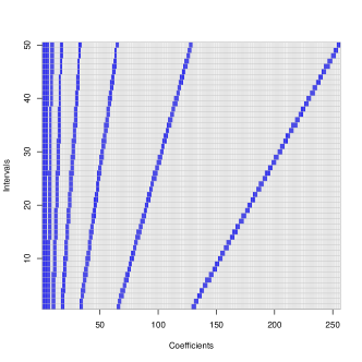
Figure 1: Correspondence between the time domain and wavelet functions for a Daubechies wavelet basis with two vanishing moments. For the time $t$, the darkest points correspond to the wavelet functions which are non null at time $t$.

3.1 Grouped variable importance for functional variables

In this section, we show how the grouped variable importance can be fruitfully used for comparing the importance of different wavelet coefficients in the context of functional prediction. Remember that $p$ functional covariates $X^{1},\dots,X^{p}$ are observed, along with a scalar response $Y$. For the sake of simplicity, covariates are decomposed on the same wavelet basis $\mathcal{B}$ but the methodology presented above could be also adapted with a specific basis for each covariate. For any $u\in\{1,\dots,p\}$, let $\mathbf{W}^{u}=(\zeta^{u},\xi^{u}_{jk})_{jk}$ be the random vector composed of the wavelet coefficients of the functional variable $X^{u}$.

Groups of wavelet coefficients

Wavelet coefficients are characterised by their frequency, time location and the functional variables they describe. Consequently, they can be grouped in many ways. We give below a nonexhaustive list of groups for which we are interested in computing the importance:

• A group related to a variable. The vector $\mathbf{W}^{u}$ defines the group $G(u)$.

• A group related to a frequency level of a variable. For a fixed variable $X^{u}$, the group is composed of the wavelet coefficients of frequency level $j$:

  $$G(j,u):=\{\xi_{j,1}^{u},\dots,\xi^{u}_{j,2^{j}-1}\}.$$

• A group related to a frequency level. The group is composed of all the wavelet coefficients of frequency level $j$ for all the variables:

  $$G(j):=\bigcup_{u=1,\dots,p}G(j,u).$$

• A group related to a given time. Define the group of “active” wavelet coefficients associated to a given time $t$ by

  $$G(t):=\bigcup_{u=1,\dots,p}\{\zeta^{u}\}\cup\bigcup_{u=1,\dots,p,\,(j,k)\in\mathcal{S}(t)}\{\xi^{u}_{jk}\}.$$

  Depending on the size of the support of $\phi$ and $\psi$, the group $G(t)$ may be very large. For instance with a Daubechies wavelet basis with two vanishing moments, in Figure 1 the group $G(t)$ is composed of the darkest points of the row corresponding to time $t$.

• A group related to a time interval. Let $[a,b]$ be a time interval. The group of “active” wavelet coefficients associated with $[a,b]$ is

  $$G([a,b]):=\bigcup_{t\in[a,b]}G(t).$$

Many other groupings could be proposed. For instance, one could regroup pairs of correlated variables, or consider a group composed of the wavelet coefficients taken in an interval of frequencies, a group related to a given time and a fixed variable, etc.

By computing the importance of such groups, one directly obtains a rough detection of the most important groups of coefficients for predicting $Y$. When grouping by frequency levels or time locations, all groups do not have equal sizes. As explained in Section 2, it is preferable to use the rescaled version of the grouped variable importance in order to compensate the effect of group size in the grouped variable importance measure.

Grouped variable selection

We now propose a more elaborate method for selecting groups of coefficients. The selection procedure is based on the Recursive Feature Elimination (RFE) algorithm proposed by Guyon et al. [2002] in the context of support vector machines. In this paper, we propose a random forests version of the RFE algorithm which is guided by grouped variable importance. The procedure is summarized in Algorithm 1. This backward grouped elimination approach produces a collection of nested subsets of groups. The selected groups are obtained by minimizing the validation error computed in step 2.

Algorithm 1 Grouped Variable Selection

1:  Train a random forest model

2:  Compute the error using a validation sample

3:  Compute the grouped variable importance measure

4:  Eliminate the least important group of variables

5:  Repeat 1–4 until no further groups remain

This algorithm is motivated by the results of our previous work [Gregorutti et al., 2014] about variable selection using the permutation importance measure for random forests. Strong correlation between predictors has a strong impact on the permutation importance measure. It was also shown in this previous paper that when predictors are strongly correlated, the RFE algorithm provides a better performance than the “non-recursive” strategy (NRFE) that computes the grouped variable importance just once and does not recompute the importance at each step of the algorithm. In the present paper, we continue this study by adapting the RFE algorithm for the grouped variable importance measure. We give below two applications of this algorithm.

• Selection of functional variables. Each vector $\mathbf{W}^{u}$ defines a group $G(u)$ and the goal is to perform a grouped variable selection over the groups $G(1),\dots,G(p)$. The selection allows us to identify the most relevant functional variables.

• Selection of wavelet levels for a given functional variable. For a fixed $u$, we make a selection over the groups $G(j,u)$ to identify the frequency levels which yield predictive information.

Remark.

Algorithm 1 for grouped variable selection is appropriate for groups defining a partition over the wavelet coefficients. This is not the case for groups related to time locations. The algorithm can not easily be adapted to these groups because most wavelet coefficients belong to several groups and the elimination of a whole group may not be an efficient strategy. For instance the coefficient $\zeta^{u}$, which approximates the smooth part of the curves and which is usually a good predictor, is common to all times $t$.

3.2 Experiments

In this section, we present various numerical experiments for illustrating the interest of grouped variable importance for analyzing functional data. We first describe the simulation set-up.

Presentation of the general simulation design

The experiments presented below consider one or several functional covariates for predicting an outcome $Y$. Except for the second simulation in Experiment 1 which is presented in detail in the next section, the functional covariates are defined as functions of $Y$.

First, an $n$-sample of the outcome variable $Y$ is simulated from a given distribution specified for each experiment. The realization of a functional covariate $X$ (denoted by $X^{u}$ when there are several) is an $n$-sample of independent discrete time random processes $X_{i}=(X_{i}(t_{\ell}))_{\ell=1,\dots,N}$, for all $i\in\{1,\dots,n\}$ under a model of the form

$$X_{i}(t_{\ell})=s(t_{\ell},Z_{i})+\sigma\varepsilon_{i,\ell},\;\ell=1,\dots,N,$$ (9)

where the $\varepsilon_{i,\ell}$ are i.i.d standard Gaussian random variables, and $t_{\ell}=\frac{\ell}{N}$. The random variable $Z_{i}$ is correlated with $Y_{i}$ and will be specified for each experiment; it is equal to the outcome variable $Y_{i}$ for most of the experiments. The functional covariates are actually simulated in the wavelet domain from the following model: for $i=1,\dots,n$, $j=0,\dots,J-1$ and $k=0,\dots,2^{j}-1$,

$$\zeta_{i}=\omega_{0}+h_{\zeta}(Z_{i})+\sigma\eta_{i\zeta},$$ (10)

and

$$\xi_{ijk}=\left\{\begin{array}[]{llll}\omega_{jk}+h_{jk}(Z_{i})+\sigma\eta_{ijk}&\mbox{ if }j\leq j^{\star},\;k\in\{0,\dots,2^{j}-1\},\\ 0&\mbox{ if }j^{\star}<j\leq J-1,\end{array}\right.$$ (11)

where $j^{\star}$ is the highest wavelet level of the signal. The random variables $\eta_{ijk}$ and $\eta_{i\zeta}$ are i.i.d. standard Gaussian. The “signal” part of Equation (11) is the sum of a random coefficient $\omega_{jk}$ whose realisation is the same for all $i$, and a link function $h_{jk}$. The coefficients $\omega_{0}$ and $\omega_{jk}$ in (10) and (11) are simulated as follows:

$$\left\{\begin{array}[]{llll}\omega_{jk}&\sim&\mathcal{N}_{1}(0,\tau_{j}^{2}),&\mbox{if }j\leq j^{\star},\;k\in\{0,\dots,2^{j}-1\},\\ \omega_{0}&\sim&\mathcal{N}_{1}(3,1),\end{array}\right.$$

where $\tau_{j}=e^{-(j-1)}$. Note that the standard deviation $\tau_{j}$ decreases with $j$ and thus less noise is added to the first wavelet levels. The link function $h_{jk}$ describes the link between the wavelet coefficients $\xi_{ijk}$ and the variable $Z$ (or the outcome variable $Y$). Two different link functions are considered in the experiments:

• a linear link: $h_{jk}(z)=\theta_{jk}z$,

• a logistic link: $h_{jk}(z)=\dfrac{\theta_{jk}}{1+e^{-z}}$,

where the coefficients $\theta_{jk}$ parametrize the strength of the relationship between $Z$ and the wavelet coefficients. The $n$ discrete processes $X_{1},\dots,X_{n}$ are simulated according to (10) and (11) before applying the inverse wavelet transform. We choose a Daubechies wavelet filter with four vanishing moments to simulate the observations. We use the same basis for the projection of the functional observations.

Experiment 1: Detection of important time intervals

In this first experiment, we illustrate the use of the grouped variable importance for detection of the most relevant time intervals. We simply estimate the importance of time intervals without applying Algorithm 1 (see Remark Remark). We only consider one functional covariate $X$ since it will be sufficient to illustrate the method. Let $\mathcal{T}^{\star}=[t_{50},t_{55}]$, we propose two simulation designs for which the outcome $Y$ is correlated to the signal $X$ on the interval $\mathcal{T}^{\star}$.

• Simulation 1. For this first simulation, we follow the general simulation design presented before by considering linear link functions $h$ for all wavelet coefficients belonging to the wavelet support $\mathcal{S}(\mathcal{T}^{\star})$. The outcome variable $Y$ is simulated from a Gaussian distribution $\mathcal{N}_{1}(0,3)$. We simulate the wavelet coefficients as in (11) and the scaling coefficients as in (10) with $Z=Y$. We take linear link functions and set $n=1000$, $\sigma=0.01$, $N=2^{8}$ and thus $J=8$. We take $j^{\star}=7$ which means that even the wavelet coefficients of highest level $j=7$ are not Dirac distributions at zero. The wavelet coefficients and the scaling coefficient are generated as follows: for any $j\in\{0,\dots,J-1\}$ and any $k\in\{0,\dots,2^{j}-1\}$,

  $$\xi_{ijk}=\left\{\begin{array}[]{lll}\omega_{jk}+Y_{i}+\sigma\eta_{ijk},&\mbox{if }(j,k)\in\mathcal{S}(\mathcal{T}^{\star})\\ \omega_{jk}+\sigma\eta_{ijk},&\mbox{otherwise,}\end{array}\right.$$ (12)

  and

  $$\zeta_{i}=\omega_{0}+Y_{i}+\sigma\eta_{i\zeta},$$ (13)

  for $i=1,\dots,n$.

• Simulation 2. In contrast to the previous simulation, we first simulate the functional variable $X$ and then simulate the outcome variable $Y$ as a function of $X$. The functional variable is simulated in the wavelet domain according to (10) and (11) with $h_{jk}=h_{\zeta}=0$ for all $j$ and $k$. We also take $n=1000$, $\sigma=0.01$, $N=2^{8}$ and $j^{\star}=7$. By applying the wavelet inverse transform for any $i$, we obtain an $n$-sample of discrete time random processes $X_{i}=(X_{i}(t_{\ell}))_{\ell=1,\dots,N}$. Figure 2 displays a set of ten of these processes.

  

  Figure 2: Experiment 1 – Example of ten processes drawn from the protocol used for Simulation 2.

  The outcome variable $Y$ is then obtained via

  $$Y_{i}=\dfrac{1000}{|\mathcal{T}^{\star}|}\sum_{t_{\ell}\in\mathcal{T}^{\star}}|X_{i}(t_{\ell})-X_{i}(t_{\ell-1})|.$$

  Thus, $Y_{i}$ is a measure of the oscillations of the curve $X_{i}$ over the interval $\mathcal{T}^{\star}$.

The aim is to detect $\mathcal{T}^{\star}$ using the grouped variable importance. In both cases, the grouped variable importance $\mathcal{I}(G(t))$ is evaluated at 50 equally spaced time points. Figure 3 displays the importance of the time points, averaged over 100 iterations. The first and third quartiles are also represented in order to highlight estimation variability. In the two cases, the importance estimation makes it possible to detect $\mathcal{T}^{\star}$.

Note that the detection problem is tricky in the second case because the link between $Y$ and the wavelet coefficients is complex here. Consequently the estimated importances are low and the important intervals are difficult to detect.

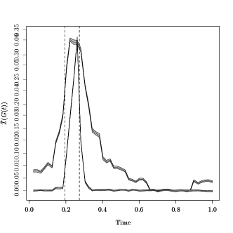
(a) Case 1

(b) Case 2

Figure 3: Experiment 1 – Averaged time importances and first and third quartiles over 100 iterations. The time interval $\mathcal{T}^{\star}$ is located between the two vertical lines.

Experiment 2: Selection of wavelet levels

This simulation deals with the selection of wavelet levels for one functional variable. We follow the general simulation design presented above. The outcome variable $Y$ is simulated from a Gaussian distribution $\mathcal{N}_{1}(0,3)$. We simulate the wavelet coefficients as in (11) and the scaling coefficients as in (10) with $Z=Y$. We perform two types of simulation:

• In the first case we use linear link functions:

  $$h_{\zeta}(y)=0.1y$$

  and

  $$h_{jk}(y)=\left\{\begin{array}[]{lll}\theta_{j}y&\mbox{ if }j\leq 3,\;k\in\{0,\dots,2^{j}-1\},\\ 0&\mbox{ otherwise,}\end{array}\right.$$

  where the $\theta_{j}$ decrease linearly from 0.1 to 0.01.

• For the second simulation, we use logistic link functions:

  $$h_{\zeta}(y)=\frac{0.1}{1+e^{-y}}$$

  and

  $$h_{jk}(y)=\left\{\begin{array}[]{lll}\dfrac{\theta_{jk}}{1+e^{-y}}&\mbox{if }j\leq 3,\;k\in\{0,\dots,2^{j}-1\},\\ 0&\mbox{ otherwise,}\end{array}\right.$$

  where the $\theta_{j}$ decrease linearly from 0.1 to 0.01.

We fix $n=1000$, $\sigma=0.05$, $N=2^{8}$ (thus $J=8$) and $j^{\star}=7$ in both cases. The aim is to identify the most relevant wavelet levels for the prediction of $Y$ using the grouped importance. We regroup the wavelet coefficients by wavelet levels: for $j\in\{0,\dots,J-1\}$,

$$G(j)=\left\{\xi_{jk},k\in\{1,\dots,2^{j}-1\}\right\}$$

and

$$G_{\zeta}=\{\zeta\}.$$

We apply Algorithm 1 with these groups. As the group sizes are different, the rescaled grouped importance criterion given in Section 2.2 is used.

The trials are both repeated 100 times. Figures 4 and 5 respectively give the results for the linear and logistic links. Let us first look at the trials with a linear link. The boxplots of the grouped permutation importances at the first step of the algorithm over the 100 trials are given in Figure  4a. The fifth group $G(3)$ being not strongly correlated with $Y$, its importance is close to zero. It is selected 40 times out of the 100 simulations (Fig. 4c) whereas $G_{\zeta}$, $G(0)$, $G(1)$ and $G(2)$ are almost always selected. The other groups are not correlated with $Y$ and are almost never selected. For each trial, the mean squared error (MSE) is computed as a function of the number of variables in the model. Figure 4b shows the average of the errors over the 100 simulations. On average, the model selected by minimizing the MSE includes four groups but the model with five groups also has an error close to the minimum.

(a)

(b)

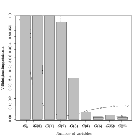
(c)

Figure 4: Experiment 2, linear links – selection of the wavelet levels. From left to right: (a) Boxplots of the grouped variable importances, (b) MSE error versus the number of groups and (c) Selection frequencies.

The simulation with the logistic link gives similar results. However the fifth group $G(3)$ is more frequently selected (Fig. 5c). The minimization of the MSE leads to the selection of five groups as shown in Figure 5b. Note that this random forest and grouped variable importance-based approach performs well even with a nonlinear link.

In both experiments, the grouped variable importances obtained at the first step of the algorithm are ranked in the same order as the $\theta_{j}$. Indeed the impact of the correlation between predictors is almost null in both cases because of the orthogonality of the wavelet bases. In this context, the backward Algorithm 1 does not provide additional information compared to the “non-recursive” strategy (see the discussion following Algorithm 1).

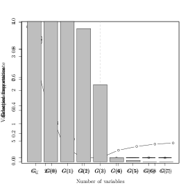
(a)

(b)

(c)

Figure 5: Experiment 2, logistic links – selection of the wavelet levels. From left to right: (a) Boxplots of the grouped variable importances, (b) MSE error versus the number of groups and (c) Selection frequencies.

Experiment 3: Selection of functional variables in the presence of strong correlation

This simulation illustrates the interest of Algorithm 1 when selecting functional variables in the presence of correlation. First, we simulate $n=1000$ i.i.d. realizations of $p=10$ functional variables $X^{1},\dots,X^{p}$ according to the general simulation design detailed before. For all $i\in\{1,\dots,n\}$, let $Z_{i}^{1},\dots,Z_{i}^{p}$ be latent variables drawn from a standard Gaussian distribution. The outcome variable $Y$ is defined as:

$$Y_{i}=3.5\,Z^{1}_{i}+3\,Z^{2}_{i}+2.5\,Z^{3}_{i}+2.5\,Z^{4}_{i}.$$

Then for $u\in\{1,\dots,p\}$, the wavelet coefficients are simulated according to (11) and (10) with a linear link:

$$\xi^{u}_{ijk}=\omega^{u}_{jk}+Z_{i}^{u}+\sigma\eta^{u}_{ijk}\quad\mbox{ if }j\leq j^{\star},\;k\in\{0,\dots,2^{j}-1\}$$

and

$$\zeta^{u}_{i}=\omega^{u}_{0}+Z_{i}^{u}+\sigma\eta^{u}_{i\zeta},$$

with $\sigma=0.1$, $N=2^{9}$ and thus $J=9$. We take $j^{\star}=3$ in order to make the functional variables smooth enough. Among the 10 variables $X^{u}$, the first four variables have decreasing predictive power whereas the others are independent of $Y$. Next, we add $q=10$ i.i.d. variables $X^{1,1},\dots,X^{1,q}$ which are strongly correlated with $X^{1}$: for any $v\in\{1,\dots,q\}$, any $i\in\{1,\dots,n\}$,

$$\zeta^{1,v}_{i}=\zeta^{1}_{i}+\tilde{\sigma}\eta^{1,v}_{i\zeta}$$

and

$$\xi_{ijk}^{1,v}=\left\{\begin{array}[]{lll}\xi_{ijk}^{1}+\tilde{\sigma}\eta^{1,v}_{ijk}&\mbox{if }j\leq j^{\star},\;k\in\{0,\dots,2^{j}-1\}\\ 0&\mbox{otherwise,}\end{array}\right.$$

where $\tilde{\sigma}=0.05$. The $\eta^{1,v}_{ijk}$ and the $\eta^{1,v}_{i\zeta}$ are i.i.d. standard Gaussian random variables. The discrete processes $X_{i}^{1,v}$ are obtained using the inverse wavelet transform. In the same way, we add $q=10$ i.i.d. variables $X^{2,1},\dots,X^{2,q}$ which are strongly correlated with $X^{2}$. To sum up, the vector of predictors is composed of 30 variables:

$$X^{1},X^{1,1},\dots,X^{1,q},X^{2},X^{2,1},\dots,X^{2,q},X^{3},X^{4},\dots,X^{p}.$$

The aim is to identify the most relevant functional variables for the prediction of $Y$. For each functional variable, we regroup all wavelet coefficients and apply Algorithm 1. This process is repeated 100 times. Boxplots of the group permutation importances at the first step of the algorithm, over the 100 trials and for each functional variable, are given in Figure 6a. We see that the importances of the variables $X^{1}$ and $X^{2}$ and their noisy replicates are much lower than those of variables $X^{3}$ and $X^{4}$. This is due to the strong correlations between the two first variables and their noisy replicates. Indeed, the importance measure decreases when the correlation or the number of correlated variables increase. Note that the importances of $X^{1}$ and $X^{2}$ are slightly lower than those of their noisy replicates. This can be explained by the fact that the correlation between $X^{1}$ and its noisy replicates is higher than, for instance, the correlation of $X^{1,1}$ with $X^{1},X^{1,2},\dots,X^{1,q}$.

Figure 6b gives a comparison of the performance of Algorithm 1 with the “non-recursive” strategy (NRFE). Algorithm 1 clearly shows better prediction performances. In particular, it reaches a minimum error faster than the NRFE: only five variables for Algorithm 1 whereas NRFE needs about twelve. The RFE procedure is more efficient than the NRFE when predictors are highly correlated.

Additional information is displayed in Figure 6c. The selection frequencies using Algorithm 1 show that the variables $X^{3}$ and $X^{4}$ are always selected. Indeed, these two variables have predictive power and they are not correlated with the other predictors. Note that $X^{1}$ and $X^{2}$ are selected less often than their replicates, even though they are more correlated with $Y$. This also comes from the fact that the correlation between $X^{1}$ and its replicates is higher than the correlation of $X^{1,1}$ with $X^{1},X^{1,2},\dots,X^{1,q}$. We observe that $X^{1}$ and $X^{2}$ are eliminated in the first steps of the backward procedure, but this has no consequence on the prediction performance of Algorithm 1. These results motivate the use of this algorithm in practice: it reduces the effect of the correlation between predictors on the selection process and provides better prediction performances.

(a)

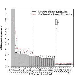
(b)

(c)

Figure 6: Experiment 3 – Selection of functional variables. From left to right: (a) Boxplots of the grouped variable importances, (b) MSE error versus the number of groups and (c) Selection frequencies using Algorithm 1.

4 A case study: variable selection for aviation safety

In this section, we study a real problem coming from aviation safety. Airlines collect large amounts of information during flights using flight data recorders. For several years now, airlines are required to use these data for flight safety purposes. A large number of flight parameters (up to 1000) are recorded each second, including aircraft speed, accelerations, the heading, position, and warning signals. Each flight provides a multivariate time series corresponding to this family of functional variables.

We focus here on the risk of long landing. A data sequence for $N=512$ seconds before touchdown is observed for predicting the landing distance. The evaluation of the risk of long landings is crucial for safety managers to avoid runway excursions and more generally to keep a high level of safety. One answer to this problem is to select the flight parameters that best explain the risk of long landings. Therefore, we attempt to find a sparse model showing good predictive performances. In the future, flight data analysis could be used for pilot training or development of new flight procedures during approach.

Following aviation experts, 23 variables are preselected, see Table 1. A sample of 1868 flights from the same airport and the same company is considered. The functional variables are projected on a Daubechies wavelet basis with four vanishing moments using the discrete wavelet transform algorithm as in Section 3. The choice of the wavelet basis is determined by the nature of the flight data, which here contains information on both the time and frequency scales.

Abbreviation	Flight parameter
AOA	angle of attack
ALT.STDC	altitude
CASC	airspeed
CASC.GSC	wind speed
DRIFT	aircraft drift angle
ELEVR, ELEVL	elevator position
FLAPC	flaps position
GLIDE.DEVC	deviation over the glide path
GW.KG	gross weight
HEAD.MAG	magnetic heading
IVV	inertial vertical speed
N11C, N12C, N21C, N22C	engine rotation speed
PITCH	rotation on the lateral axis
PITCH.RATE	aircraft pitch rate
ROLL	rotation on the longitudinal axis
RUDD	rudder position
SAT	static air temperature
VAPP	approach speed
VRTG	vertical acceleration

Table 1: List of preselected flight parameters.

Preliminary dimension reduction

The design matrix formed by the wavelet coefficients for all of the chosen flight parameters has dimension $23\times 512=11~{}776$. Selecting the variables directly from the whole set of coefficients is computationally prohibitive, so we first need to significantly reduce the dimension. The naive method that shrinks the $n$ curves independently according to Donoho and Johnstone [1994] and then brings the non-zero coefficients together in a second step would lead us to consider a large block of coefficients with many zero values. This is not relevant in our context, so we propose an alternative method which consists of shrinking the wavelet coefficients of the $n$ curves simultaneously. More precisely, this method is adapted from Donoho and Johnstone [1994] for the particular context of $n$ independent (but not necessary identically distributed) discrete random processes. Shrinkage is performed on the norm of the $n$-dimensional vector containing the wavelet coefficients. The complete method is described in C.

Selection of flight parameters

We obtain a selection of the functional parameters by grouping together the wavelet coefficients of each flight parameter and applying Algorithm 1 with these groups. At each iteration, we randomly split the dataset into a training set containing 90 % of the data and a validation set containing the remaining 10 %. In the backward algorithm, the grouped variable importance is computed on the training set and the validation set is only used to compute the MSE errors. The selection procedure is repeated 100 times to reduce the variability of the selection. The final model is chosen by minimizing the averaged prediction error. Figure 7a represents the boxplots of the grouped variable importance values computed on the 100 runs of the selection algorithm. According to this ranking, five variables are found to be significantly relevant. Looking at the averaged MSE estimate on Figure 7b, we see that the average number of selected variables is ten, but taking only five is sufficient to get a risk close to the minimum.

Figure 7c gives additional information, displaying the proportion of times each flight parameter is selected. First, it confirms the previous remarks: five variables are always selected by the algorithm and the first ten are selected more than 60 times over the 100 runs. Second, it shows that flight parameters related to aircraft trajectory during approach are among the most relevant for predicting long landings. Indeed, the elevators (ELEVL, ELEVR) are used by the pilots to control the pitch of the aircraft. These have an effect on the angle of attack (AOA) and consequently on the landing. The variable GLIDE.DEVC is the glide slope deviation, i.e., the deviation between the aircraft trajectory and a glide path of approximatively three degrees above horizontal. Other significant variables are the gross weight (GW.KG) which has an effect on the deceleration efficiency, the airspeed (CASC) and the engine rating (N11C, N12C).

(a)

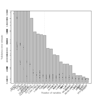
(b)

(c)

Figure 7: Application to long landings – from left to right: (a) Boxplots of the grouped variable importance, (b) MSE error versus the number of groups and (c) selection frequencies.

It should be noted that the ranking based on selection frequency is close to the direct ranking given by the importance measures when all variables are included in the model. This suggests that for this data, correlation between predictors is not strong enough to influence their permutation importance measures. Moreover, if we regroup several variables such as for example flight parameters N11C and N12C, N21C and N22C, and ELEVR and ELEVL into three new variables N1, N2 and ELEV, Figure 8 shows that the ranking remains unchanged.

(a)

(b)

Figure 8: Application to long landings – grouped variable importance measured before and after grouping the correlated flight parameters N11C and N12C, N21C and N22C, ELEVR and ELEVL, as N1, N2 and ELEV.

Selection of wavelet levels

We now determine, for a given flight parameter, which wavelet levels are the most able to predict the risk of long landing. We perform selection of wavelet levels independently for the gross weight (GW.KG) and angle of attack (AOA), which are among the most commonly selected flight parameters. Figures 9a and 9c show that the average number of selected levels for GW.KG is less than for AOA. Indeed, the selection frequencies in Figure 9b indicate that for GW.KG, the first approximation levels are selected at each run (groups $\zeta,G(0)$ and $G(1)$) whereas the last levels are selected in less than 40 of the 100 trials. The situation is quite different for AOA: all levels are selected more than 50 times. The predictive power of this functional variable is contained in both the high levels of approximation and in the details of the wavelet decomposition (Fig. 9d).

(a) Gross weight – MSE versus the number of groups

(b) Gross weight – Selection frequencies

(c) Angle of attack – MSE versus the number of groups

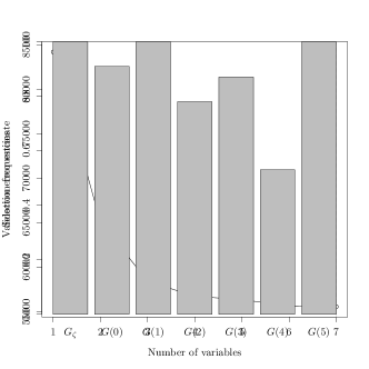
(d) Angle of attack – Selection frequencies

Figure 9: Application to long landings – selection of wavelet levels for the gross weight and angle of attack.

Detection of important time intervals

The importance of time interval is now computed for two of the most important flight parameters, the altitude (ALT.STDC) and angle of attack (AOA). Figure 10 displays the averaged grouped importance $G(t)$ evaluated on 50 equally-spaced time points. This number is arbitrarily chosen in order to find a tradeoff between computational time and accuracy. The time $t=0$ refers to touchdown of the aircraft.

Two intervals are detected with high predictive power for the altitude. These results are consistent with the view of aviation safety experts. Indeed, during the interval $[-460,-400]$, the aircraft has to level off for stabilizing before the final approach. An overly high altitude at this moment can induce a long landing. During the interval $[-60,0]$, the final seconds before touchdown, an overly high altitude can also induce a long landing.

The interval detected for the angle of attack is $[-200,-100]$. This make sense because according to flight procedure pilots have to reduce the vertical speed a few seconds before touchdown (the flare). Consequently, they must increase the angle of attack in order to keep sufficient lift.

(a) Altitude

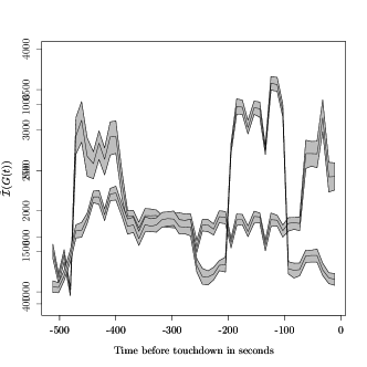
(b) Angle of attack

Figure 10: Application to long landings – averaged time importance and first and third quartiles over 100 trials.

5 Conclusion

We have considered the selection of grouped variables using random forests and proposed a new permutation-based importance measure for groups of variables. Our theoretical analysis provided exact decompositions of the grouped importance measure into a sum of the individual importances for specific models such as additive regression models. A simulation study highlighted the fact that in general the importance of a group does not reduce to the sum of the individual importances. Since the idea of variable importance is not restricted to the random forest algorithm, it would be of interest to extend our method to other learning algorithms such as different bagging methods, neural networks and SVMs.

We have also introduced a rescaled version of the grouped variable importance with a heuristic choice for the normalization factor. The question of choosing a good value for the normalization factor is an open question that could perhaps be examined with further mathematical work.

The second contribution of the article was an original method for selecting functional variables using the grouped variable importance measure and a projection-based approach. The various functional variables were projected onto a wavelet basis and the corresponding coefficients grouped in different ways. For instance, one can choose to regroup all coefficients of a given functional variable. The selection of these groups involved selection of the functional variables. Various other groupings were proposed for wavelet decompositions. A backward algorithm adapted from recursive feature elimination in the context of random forests was used as a selection algorithm. The selection process was guided by the grouped importance measure in order to select the most relevant group of variables for predicting the variable of interest.

Lastly, an extensive simulation study was performed to illustrate application of the grouped importance measure for functional data analysis, and encouraging results were then obtained for a real life problem in aviation safety. Of course, the grouped variable importance measure may be used for any other application as soon as the features can be partitioned into known disjoint pieces. Potential applications can be found in the extensive literature about the group lasso method [Yuan and Lin, 2006b], see for instance Meier et al. [2008], Ma et al. [2007] for applications in Genetics and Chatterjee et al. [2012] for applications in Climatology.

Appendix A Proof of Proposition 1

The vector $\mathbf{X}^{\prime}_{J}$ and the vector $\mathbf{X}_{(J)}$ are defined as in Section 2. We have

$$\mathcal{I}(\mathbf{X}_{J}) =\mathbb{E}[(Y-f(\mathbf{X})+f(\mathbf{X})-f(\mathbf{X}_{(J)}))^{2}]-\mathbb{E}[(Y-f(\mathbf{X}))^{2}]$$

$$=\mathbb{E}[(f(\mathbf{X})-f(\mathbf{X}_{(J)}))^{2}]+2\mathbb{E}\left[\varepsilon(f(\mathbf{X})-f(\mathbf{X}_{(J)}))\right]$$

$$=\mathbb{E}[(f(\mathbf{X})-f(\mathbf{X}_{(J)}))^{2}],$$

since $\mathbb{E}[\varepsilon f(\mathbf{X})]=\mathbb{E}[f(\mathbf{X})\mathbb{E}[\varepsilon|\mathbf{X}]]=0$ and $\mathbb{E}[\varepsilon f(\mathbf{X}_{(J)}]=\mathbb{E}(\varepsilon)\mathbb{E}[f(\mathbf{X}_{(J)}]=0$. Since $f(\mathbf{X})=f_{J}(\mathbf{X}_{J})+f_{\bar{J}}(\mathbf{X}_{\bar{J}})$, we find that

$$\mathcal{I}(\mathbf{X}_{J}) =\mathbb{E}[(f_{J}(\mathbf{X}_{J})-f_{J}(\mathbf{X}^{\prime}_{J}))^{2}]$$

$$=2\operatorname*{Var}[f_{J}(\mathbf{X}_{J})],$$

as $\mathbf{X}_{J}$ and $\mathbf{X}^{\prime}_{J}$ are independent and identically distributed.

Appendix B Additional experiments on the grouped variable importance

In this section, we investigate the properties of the permutation importance measure of groups of variables with numerical experiments, in addition to the theoretical results given before. In particular, we compare this quantity with the sum of individual importances in various models. We also study how this quantity behaves in “sparse situations” where only a small number of variables in the group are relevant for predicting the outcome.

The general framework of the experiments is the following. For a fixed $p\geq 1$, define $\mathbf{X}^{\top}:=(\mathbf{W}^{\top},\mathbf{Z}^{\top})$ where $\mathbf{W}$ and $\mathbf{Z}$ are random vectors both of length $p$. Some of the components of $\mathbf{W}$ are correlated with $Y$ whereas those in $\mathbf{Z}$ are all independent of $Y$. Let $\textbf{C}_{w}$ be the variance-covariance matrix of $\mathbf{W}$. By incorporating the group $\mathbf{Z}$ in the model, we present a realistic framework where not all the $X_{j}$ have a link with $Y$. For each experiment, we simulate $n=1000$ samples of $Y$ and $\mathbf{X}$ and compute the importance $\mathcal{I}(\mathbf{W})$ of the group $\mathbf{W}$, the rescaled grouped variable importance $\mathcal{I}_{\textrm{nor}}(\mathbf{W})$ and the sum of the individual importances of the variables in $\mathbf{W}$. We repeat each experiment 500 times. The boxplots of the importances over the 500 repetitions are shown in Figures 11 to 14 with values $p$ between 1 and 16.

Let $\textbf{0}_{p}$ and $\textbf{I}_{p}$ denote the null vector and identity matrix of $\mathbb{R}^{p}$. Let $\mathbbm{1}_{p}$ be the vector in $\mathbb{R}^{p}$ with all coordinates equal to one and let $\textbf{0}_{p,q}$ denote the null matrix of dimension $p\times q$.

Experiment 1: linear link function.

We simulate $\mathbf{X}$ and $Y$ from a multivariate Gaussian distribution. More precisely, we simulate samples from the joint distribution

$$\begin{pmatrix}\mathbf{X}\\ Y\end{pmatrix}=\begin{pmatrix}\mathbf{W}\\ \mathbf{Z}\\ Y\end{pmatrix}\sim\mathcal{N}_{2p+1}\left(\textbf{0}_{2p+1}\,,\,\begin{pmatrix}\textbf{C}_{w}&\textbf{0}_{p,p}&\boldsymbol{\tau}\\ \textbf{0}_{p,p}&\textbf{I}_{p}&\textbf{0}_{p}\\ \boldsymbol{\tau}^{\top}&\textbf{0}_{p}^{\top}&1\end{pmatrix}\right),$$

where $\boldsymbol{\tau}$ is the vector of the covariances between $\mathbf{W}$ and $Y$. In this context, the conditional distribution of $Y$ over $\mathbf{X}$ is normal and the conditional mean $f$ is a linear function: $f(\mathbf{x})=\sum_{j=1}^{p+q}\alpha_{j}x_{j}$ with $\alpha=(\alpha_{1},\ldots,\alpha_{p},0,\dots,0)^{\top}$ a sequence of deterministic coefficients (see for instance Rao [1973], p. 522.

• Experiment 1a: independent predictors. We take $\boldsymbol{\tau}=0.9\,\mathbbm{1}_{p}$ and $\textbf{C}_{w}=\textbf{I}_{p}$. All variables of $\mathbf{W}$ are independent and correlated with $Y$.

• Experiment 1b: correlated predictors. We take $\boldsymbol{\tau}=0.9\,\mathbbm{1}_{p}$ and $\textbf{C}_{w}=(1-0.9)\textbf{I}_{p}+0.9\mathbbm{1}_{p}\mathbbm{1}_{p}^{\top}$. The variables of $\mathbf{W}$ are correlated, and also correlated with $Y$.

• Experiment 1c: independent predictors, sparse case. We take $\boldsymbol{\tau}=(0.9,0,\dots,0)^{\top}$ and $\textbf{C}_{w}=\textbf{I}_{p}$. Only the first variable in the group $\mathbf{W}$ is correlated with $Y$.

• Experiment 1d: correlated predictors, sparse case. We take $\boldsymbol{\tau}=(0.9,0,\dots,0)^{\top}$ and $\textbf{C}_{w}=(1-0.9)\textbf{I}_{p}+0.9\mathbbm{1}_{p}\mathbbm{1}_{p}^{\top}$. The variables of $\mathbf{W}$ are correlated. Only the first variable in the group $\mathbf{W}$ is correlated with $Y$.

Experiment 2: additive link function.

We simulate $\mathbf{X}$ from a multivariate Gaussian distribution:

$$\mathbf{W}=\begin{pmatrix}\mathbf{W}\\ \mathbf{Z}\\ \end{pmatrix}\sim\mathcal{N}_{2p}\left(\textbf{0}_{2p}\,,\,\begin{pmatrix}\textbf{C}_{w}&\textbf{0}_{p,p}\\ \textbf{0}_{p,p}&\textbf{I}_{p}\end{pmatrix}\right),$$

and the conditional distribution of $Y$ is

$$(Y|\mathbf{X})\sim\mathcal{N}\left(\sum_{j=1}^{p}f_{j}(X_{j}),1\right),$$

where $f_{j}(x)=\sin(2x)+j$ for $j<p/2$ and $f_{j}(x)=\cos(2x)+j$ for $j\geq p/2$.

• Experiment 2a: independent predictors. We take $\textbf{C}_{w}=\textbf{I}_{p}$. All variables of $\mathbf{W}$ are independent and correlated with $Y$.

• Experiment 2b: correlated predictors. We take $\textbf{C}_{w}=(1-0.9)\textbf{I}_{p}+0.9\mathbbm{1}_{p}\mathbbm{1}_{p}^{\top}$. The variables of $\mathbf{W}$ are correlated and also correlated with $Y$.

Experiment 3: link function with interactions.

We simulate $\mathbf{X}$ from a multivariate Gaussian distribution:

$$\mathbf{W}=\begin{pmatrix}\mathbf{W}\\ \mathbf{Z}\\ \end{pmatrix}\sim\mathcal{N}_{2p}\left(\textbf{0}_{2p}\,\textbf{I}_{2p}\right),$$

and the conditional distribution of $Y$ is

$$(Y|\mathbf{X})\sim\mathcal{N}\left(\sum_{j=1}^{p}X_{j}+X_{p}X_{1}+\sum_{j=1}^{p-1}X_{j}X_{j+1}\,,\,1\right).$$

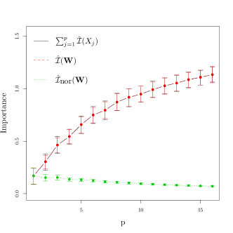
(a) Experiment 1a

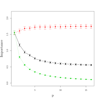
(b) Experiment 1b

Figure 11: Boxplots of the importance measures for Experiments 1a and 1b. The number of variables in $\mathbf{W}$ varies from 1 to 16. For Experiment 1a, the sum of the individual importance@s and $\hat{\mathcal{I}}(\mathbf{W})$ overlap.

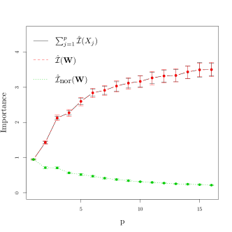
(a) Experiments 2a

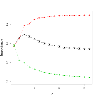
(b) Experiments 2b

Figure 12: Boxplots of the importance measures for Experiments 2a and 2b. The number of variables in $\mathbf{W}$ varies from 1 to 16. For Experiment 2a, the sum of the individual importances and $\hat{\mathcal{I}}(\mathbf{W})$ overlap.

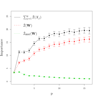
Figure 13: Boxplots of the importance measures for Experiment 3. The number of variables in $\mathbf{W}$ varies from 1 to 16.

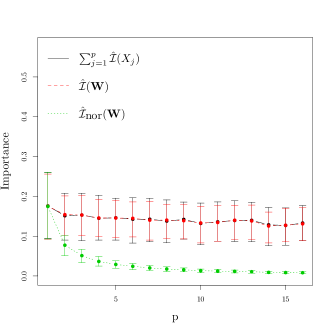
(a) Experiment 1c

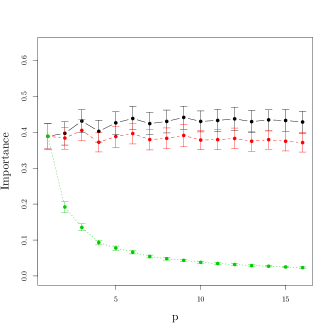
(b) Experiment 1d

Figure 14: Boxplots of the importance measures for Experiments 1c and 1d. The number of variables in $\mathbf{W}$ varies from 1 to 16. For Experiment 2a, the sum of the individual importances and $\hat{\mathcal{I}}(\mathbf{W})$ overlap.

Results

Experiments 1a-b and 2a-b illustrate the results of Corollary 1 (see Figures 11 and 12). Indeed, the regression function in both cases satisfies the additive property (3) for these experiments. In Experiments 1a and 2a, the variables of the group $\mathbf{W}$ are independent and the grouped variable importance is nothing more than the sum of the individual importances in this case. In Experiments 1b and 2b, the variables of group $\mathbf{W}$ are positively correlated. In these situations, the grouped variable importance is larger than the sum of the individual importances, which agrees with Equation 4. Note that the grouped variable importance increases with $p$, which is natural because the amount of information for predicting $Y$ increases with the group size in these models. On the other hand, it was shown in Gregorutti et al. [2014] that individual importances decrease with correlation between the predictors. Indeed we observe that the sum of the individual importances decreases with $p$ in the correlated cases.

The regression function in Experiment 3 does not satisfy the additive form (3). Although the variables in the group are independent, the grouped variable importance is not equal to the sum of the individual importances (Figure 13). In a general setting therefore, it appears that these two quantities differ.

We now comment the results of the sparse Experiments 1c and 1d (Figure 14). It is clear that $\mathcal{I}(\mathbf{W})=\mathcal{I}(X_{1})=\sum_{j=1\dots p}\mathcal{I}(X_{j})$ for these two experiments (see Proposition 1 for instance). Regarding Experiment 1c, the boxplots of the estimated values $\hat{\mathcal{I}}(\mathbf{W})$ and $\sum_{j=1\dots p}\hat{\mathcal{I}}(X_{j})$ agree with this equality. On the other hand, in Experiment 1d, we observe that $\sum_{j=1\dots p}\hat{\mathcal{I}}(X_{j})$ is significantly higher than $\hat{\mathcal{I}}(\mathbf{W})$. Indeed, it has been noticed by Nicodemus et al. [2010] that the individual importances of predictors that are not associated with the outcome tend to be overestimated by random forests when there correlation between predictors. In contrast, the estimator $\hat{\mathcal{I}}(\mathbf{W})$ seems to correctly estimate $\mathcal{I}(\mathbf{W})$ even for large $p$. Indeed, for both experiments 1c and 1d, the importance $\hat{\mathcal{I}}(\mathbf{W})$ is unchanged when the size of the group $p$ varies from 2 to 16. Note that for variable selection, we may prefer to consider the rescaled importance $\hat{\mathcal{I}}_{\textrm{nor}}$ so as to select with priority small groups of variables.

Appendix C Curve dimension reduction with wavelets

The analysis of flight data in Section 4 required, for computational reasons, to preliminarily reduce the dimension of the wavelet decomposition of the flight parameters. We require to adapt the well-known wavelet shrinkage method to the context of independent random processes. Using the notation of Section 3, we first recall the hard-thresholding estimator introduced by Donoho and Johnstone [1994] in the case of one random signal. This approach is then extended to deal with $n$ independent random signals.

Signal denoising via wavelet shrinkage

The problem of signal denoising can be summarized as follows. Suppose that we observe $N$ noisy samples $X(t_{1}),\dots,X(t_{N})$ of a deterministic function $s$ (the signal):

$$X(t_{\ell})=s(t_{\ell})+\sigma\varepsilon_{\ell},\quad\ell=1,\ldots,N,$$ (14)

where the $\varepsilon_{\ell}$ are independent standard Gaussian random variables. We assume that $s$ belongs to $L^{2}([0,1])$. The goal is to recover the underlying function $s$ from the noisy data $\{X(t_{\ell}),\ell\in\{1,\dots,N\}\}$ with small error. Using the discrete wavelet transform, this model can be rewritten in the wavelet domain as

$$\xi_{jk}=\omega_{jk}+\sigma\eta_{jk},\quad\forall j\in\{0,\dots,J-1\},\,\forall k\in\{0,\dots,2^{j}-1\},$$

and the scaling domain as

$$\zeta=\omega_{0}+\sigma\eta_{0},$$

where $\xi_{jk}$ and $\zeta$ are the empirical wavelet and scaling coefficients of $X(t_{\ell})$ as in Equation (8). The random variables $\eta_{jk}$ and $\eta_{0}$ are i.i.d. random variables from the distribution $\mathcal{N}_{1}(0,1)$.

A natural approach for estimating $\omega_{jk}$ is to shrink the coefficients $\xi_{jk}$ to zero. An estimator of $s$ in this context has the form

$$\hat{s}(t_{\ell})=\hat{\omega}_{0}\phi(t_{\ell})+\sum_{j=0}^{J-1}\sum_{k=0}^{2^{j}-1}\hat{\omega}_{jk}\psi_{jk}(t_{\ell}),$$ (15)

with $\hat{\omega}_{0}=\zeta$ and

$$\hat{\omega}_{jk}=\left\{\begin{array}[]{lll}\xi_{jk}&\mbox{ if }|\xi_{jk}|>\delta_{N}\\ 0&\mbox{ otherwise.}\end{array}\right.$$

This method is referred to as the hard-thresholding estimator in the literature. Donoho and Johnstone [1994] propose the universal threshold $\delta_{N}=\sigma\sqrt{2\log(N)}$. In addition, the standard deviation $\sigma$ can be estimated by the median absolute deviation (MAD) estimate of the wavelet coefficients at the finest levels, i.e.,

$$\hat{\sigma}=\dfrac{\mbox{Med}(|\xi_{jk}-\mbox{Med}(\xi_{jk})|:j=J-1,k=0,\dots,2^{J-1}-1)}{0.6745},$$

where the normalisation factor 0.6745 comes from the normality assumption in (14). This estimator is known to be a robust and consistent estimator of $\sigma$. The underlying idea is that the variability in the wavelet coefficients is essentially concentrated at the finest level.

Consistent wavelet thresholding for independent random signals

$\bullet$ Identically distributed case

We start by assuming that the observations come from the same distribution: for any $i\in\{1,\dots,n\}$,

$$X_{i}(t_{\ell})=s(t_{\ell})+\sigma\varepsilon_{i,\ell},\quad\ell=1,\ldots,N,$$ (16)

where the $\varepsilon_{i,\ell}$ are independent standard Gaussian random variables. The wavelet coefficients of $s$ can be easily deduced from the mean signal $\bar{X}:=\frac{1}{n}\sum_{i=1}^{n}X_{i}$ which satisfies

$$\bar{X}(t_{\ell})=s(t_{\ell})+\frac{\sigma}{\sqrt{n}}\varepsilon_{\ell},\quad\ell=1,\ldots,N,$$

where the $\varepsilon_{\ell}$ are independent standard Gaussian random variables. By applying the hard-thresholding rule to this signal, we obtain the following estimation of the wavelet parameters of $s$: $\hat{\omega}_{0}=\zeta$ and

$$\hat{\omega}_{jk}=\left\{\begin{array}[]{lll}\bar{\xi}_{jk}&\mbox{ if }|\bar{\xi}_{jk}|>\bar{\delta}_{N}\\ 0&\mbox{ otherwise,}\end{array}\right.$$

where $\bar{\xi}_{jk}$ is the wavelet coefficient of level $(j,k)$ of $\bar{X}$. Here the threshold is $\bar{\delta}_{N}=\frac{\sigma}{\sqrt{n}}\sqrt{2\log(N)}$.

$\bullet$ Non identically distributed case

In many real life situations, assuming that the $n$ signals are identically distributed is not a realistic assumption. For the study presented in Section 4 for instance, the flight parameters have no reason to follow the same distribution in safe and unsafe conditions. We propose a generalization of the model (16) by introducing a latent random variable $Z$ taking its values in a set $\mathcal{Z}$. Roughly speaking, the variable $Z$ represents all the phenomena that have an effect on the mean signal. Conditionally on $Z_{i}=z_{i}$, the distribution of the process $X_{i}$ is now defined, for any $i\in\{1,\dots,n\}$, by

$$X_{i}(t_{\ell})=s(t_{\ell},z_{i})+\sigma\varepsilon_{i,\ell}\,,\quad\ell=1,\ldots,N,$$ (17)

where the $\varepsilon_{i,\ell}$ are independent standard Gaussian random variables. This regression model allows us to consider various situations of interest arising in functional data analysis. In supervised settings where a variable $Y$ has to be predicted using $X$, one reasonable model is to take $Z=Y$. We now propose a hard-thresholding method which simultaneously shrinks the wavelet decomposition of the $n$ signals.

Let $\|\cdot\|_{n}$ denote the $\ell_{2}$-norm in $\mathbb{R}^{n}$: $\|\boldsymbol{u}\|_{n}:=\sqrt{\sum_{i=1}^{n}u_{i}^{2}}$ for any $\boldsymbol{u}\in\mathbb{R}^{n}$. Let $\boldsymbol{\xi}_{jk}$ be the vector $(\xi_{1jk},\dots,\xi_{ijk},\dots,\xi_{njk})^{\top}$ where $\xi_{ijk}$ is the coefficient of level $(j,k)$ in the wavelet decomposition of the signal $X_{i}$. For any $z\in\mathcal{Z}$, let $\omega_{jk}(z)$ be the wavelet coefficient of level $(j,k)$ of $s(\cdot,z)$, and $\boldsymbol{\omega}_{jk}:=(\omega_{jk}(Z_{1}),\dots,\omega_{jk}(Z_{n}))^{\top}$. We define the common wavelet support of $s$ by

$$L:=\left\{(j,k)\,|\,\omega_{jk}(Z)=0\>a.s.\right\}.$$

If $(j,k)\in L$, then $\boldsymbol{\omega}_{jk}=(0,\dots,0)^{\top}$ almost surely and $\|\boldsymbol{\xi}_{jk}\|_{n}^{2}$ has a centered chi-square distribution with $n$ degrees of freedom. Otherwise, $\boldsymbol{\omega}_{jk}$ can be non null and in this case $\|\boldsymbol{\xi}_{jk}\|_{n}^{2}$ has the distribution of a sum of $n$ independent uncentered chi-square distributions. We can thus propose a thresholding rule for the statistic $\|\boldsymbol{\xi}_{jk}\|_{n}$. For any $j\in\{0,\dots,J-1\}$ and any $k\in\{0,\dots,2^{j}-1\}$, let

$$\hat{\boldsymbol{\omega}}_{jk}=\left\{\begin{array}[]{ll}\boldsymbol{\xi}_{jk}&\mbox{ if }\|\boldsymbol{\xi}_{jk}\|_{n}>\delta_{N,n}\\ (0,\dots,0)^{\top}&\mbox{ otherwise,}\end{array}\right.$$ (18)

where the threshold $\delta_{N,n}$ depends on $N,n$ and $\sigma$. Proving adaptive results in the spirit of Donoho et al. [1995] for this method is beyond the scope of the paper. However, an elementary consistent result can be proved. We would like $\hat{\boldsymbol{\omega}}_{jk}$ to be a zero vector with high probability when $(j,k)\in L$. For some $x\geq 0$, take $\delta^{2}_{N,n}=\delta_{N,n}^{2}(x)=\sigma^{2}(2x+2\sqrt{nx}+n)$. Then,

$$\mathbb{P}\left[\bigcup_{(j,k)\in L}\,\left\{\hat{\boldsymbol{\omega}}_{jk}\neq(0,\dots,0)^{\top}\right\}\right] \leq \sum_{(j,k)\in L}\mathbb{P}\left[\|\boldsymbol{\xi}_{jk}\|^{2}_{n}\geq\delta^{2}_{N,n}(x)\right]$$ (19)

$$= \sum_{(j,k)\in L}\mathbb{P}\left[\dfrac{\|\boldsymbol{\xi}_{jk}\|_{n}^{2}}{\sigma^{2}}-n\geq 2x+2\sqrt{nx}\right]$$

$$\leq |\bar{L}|e^{-x}\leq Ne^{-x},$$

where we have used a deviation bound for central chi-square distributions from Laurent and Massart [2000, p. 1325]. If the signal is exactly zero, it can be recovered with high probability by taking $x\gg\log(N)$. In particular, if we choose $x=2\log(N)$, the threshold is $\delta_{N,n}^{2}=\sigma^{2}(4\log(N)+2\sqrt{2n\log(N)}+n)$ and the convergence rate in (19) is of order $O(\frac{1}{N})$. In practice, $\sigma$ can be estimated by a MAD estimator computed on the coefficients of the highest level of all $n$ wavelet decompositions. Next, $x$ and $\delta_{N,n}$ can be chosen such that (19) is lower than a given probability $q$. Letting $Ne^{-x}=q$, we obtain the threshold

$$\delta_{N,n}=\hat{\sigma}\left(2\log\left(\dfrac{N}{q}\right)+2\sqrt{n\log\left(\dfrac{N}{q}\right)}+n\right)^{\frac{1}{2}}.$$

Assuming that $\omega_{j,k}(Z)=0$ almost surely for some level $(j,k)$ is a strong assumption that is difficult to meet in practice. It can be hoped that this method still works if the wavelet support of $s(\cdot,z)$ does not vary too much with $z$. In particular, it may be applied if there exists a common set $S$ of indices $(j,k)$ such that, for any $z$, the projection of $s(\cdot,z)$ on $\mbox{Vect}(\psi_{jk}\,|\,(j,k)\in S)$ is not too far from $s(\cdot,z)$ for the $L^{2}$ norm.

References

References

- Amato et al. [2006] Amato, U., Antoniadis, A., De Feis, I., 2006. Dimension reduction in functional regression with applications. Computational Statistics and Data Analysis 50, 2422–2446.
- Antoniadis et al. [2001] Antoniadis, A., Bigot, J., Sapatinas, T., 2001. Wavelet estimators in nonparametric regression: A comparative simulation study. Journal of Statistical Software , 1–83.
- Araki et al. [2009] Araki, Y., Konishi, S., Kawano, S., Matsui, H., 2009. Functional logistic discrimination via regularized basis expansions. Communications in Statistics, Theory and Methods 38, 2944–2957.
- Biau et al. [2005] Biau, G., Bunea, F., Wegkamp, M., 2005. Functional classification in hilbert spaces. IEEE Transactions on Information Theory 51, 2163–2172.
- Breiman [1996] Breiman, L., 1996. Bagging predictors. Machine Learning 24, 123–140.
- Breiman [2001] Breiman, L., 2001. Random forests. Machine Learning 45, 5–32.
- Breiman et al. [1984] Breiman, L., Friedman, J.H., Olshen, R.A., Stone, C.J., 1984. Classification and regression trees. Wadsworth Advanced Books and Software.
- Cai and Hall [2006] Cai, T., Hall, P., 2006. Prediction in functional linear regression. The Annals of Statistics 34, 2159–2179.
- Cardot et al. [1999] Cardot, H., Ferraty, F., Sarda, P., 1999. Functional linear model. Statistics and Probability Letters 45, 11–22.
- Cardot et al. [2003] Cardot, H., Ferraty, F., Sarda, P., 2003. Spline estimators for the functional linear model. Statistica Sinica 13, 571–592.
- Chakraborty and Pal [2008] Chakraborty, D., Pal, N.R., 2008. Selecting useful groups of features in a connectionist framework. IEEE Transactions on Neural Networks 19, 381–396.
- Chatterjee et al. [2012] Chatterjee, S., Steinhaeuser, K., Banerjee, A., Chatterjee, S., Ganguly, A.R., 2012. Sparse group lasso: Consistency and climate applications., in: SDM, SIAM. pp. 47–58.
- Díaz-Uriarte and Alvarez de Andrés [2006] Díaz-Uriarte, R., Alvarez de Andrés, S., 2006. Gene selection and classification of microarray data using random forest. BMC Bioinformatics 7, 3.
- Donoho and Johnstone [1994] Donoho, D.L., Johnstone, I.M., 1994. Ideal spatial adaptation by wavelet shrinkage. Biometrika 81, 425–455.
- Donoho et al. [1995] Donoho, D.L., Johnstone, I.M., Kerkyacharian, G., Picard, D., 1995. Wavelet shrinkage: asymptopia. Journal of the Royal Statistical Society, Series B 57, 301–369.
- Fan and James [2013] Fan, Y., James, G., 2013. Functional additive regression. Preprint.
- Ferraty [2011] Ferraty, F. (Ed.), 2011. Recent Advances in Functional Data Analysis and Related Topics. Springer-Verlag.
- Ferraty and Vieu [2006] Ferraty, F., Vieu, P., 2006. Nonparametric Functional Data Analysis: Theory and Practice (Springer Series in Statistics). Springer-Verlag New York, Inc.
- Fromont and Tuleau [2006] Fromont, M., Tuleau, C., 2006. Functional classification with margin conditions, in: 19th Annual Conference on Learning Theory.
- Genuer et al. [2010] Genuer, R., Poggi, J.M., Tuleau-Malot, C., 2010. Variable selection using random forests. Pattern Recognition Letters 31, 2225–2236.
- Górecki and Smaga [2015] Górecki, T., Smaga, L., 2015. A comparison of tests for the one-way anova problem for functional data. Computational Statistics , 1–24.
- Gregorutti et al. [2014] Gregorutti, B., Michel, B., Saint Pierre, P., 2014. Correlation and variable importance in random forests. ArXiv:1310.5726.
- Guyon and Elisseeff [2003] Guyon, I., Elisseeff, A., 2003. An introduction to variable and feature selection. The Journal of Machine Learning Research 3, 1157–1182.
- Guyon et al. [2002] Guyon, I., Weston, J., Barnhill, S., Vapnik, V., 2002. Gene selection for cancer classification using support vector machines. Machine Learning 46, 389–422.
- He and Yu [2010] He, Z., Yu, W., 2010. Stable feature selection for biomarker discovery. Computational biology and chemistry 34, 215–225.
- Laurent and Massart [2000] Laurent, B., Massart, P., 2000. Adaptive estimation of a quadratic functional by model selection. The Annals of Statistics 28, 1245–1501.
- Ma et al. [2007] Ma, S., Song, X., Huang, J., 2007. Supervised group lasso with applications to microarray data analysis. BMC bioinformatics 8, 60.
- Matsui [2014] Matsui, H., 2014. Variable and boundary selection for functional data via multiclass logistic regression modeling. Computational Statistics and Data Analysis 78, 176 – 185.
- Matsui and Konishi [2011] Matsui, H., Konishi, 2011. Variable selection for functional regression models via the regularization. Computational Statistics and Data Analysis 55, 3304–3310.
- Meier et al. [2008] Meier, L., Van De Geer, S., Bühlmann, P., 2008. The group lasso for logistic regression. Journal of the Royal Statistical Society: Series B (Statistical Methodology) 70, 53–71.
- Nicodemus et al. [2010] Nicodemus, K.K., Malley, J.D., Strobl, C., Ziegler, A., 2010. The behaviour of random forest permutation-based variable importance measures under predictor correlation. BMC Bioinformatics 11, 110.
- Percival and Walden [2000] Percival, D.B., Walden, A.T., 2000. Wavelet Methods for Time Series Analysis. Cambridge University Press.
- Poggi and Tuleau [2006] Poggi, J.M., Tuleau, C., 2006. Classification supervisée en grande dimension. application à l’agrément de conduite automobile. Revue de Statistique Appliquée 4, 39–58.
- Ramsay and Silverman [2005] Ramsay, J.O., Silverman, B.W., 2005. Functional Data Analysis. Springer Series in Statistics, Springer.
- Rao [1973] Rao, C.R., 1973. Linear statistical inference and its applications. Wiley series in probability and mathematical statistics: Probability and mathematical statistics, Wiley.
- Rossi et al. [2006] Rossi, F., François, D., Wertz, V., Verleysen, M., 2006. A functional approach to variable selection in spectrometric problems, in: Proceedings of 16th International Conference on Artificial Neural Networks, ICANN 2006, pp. 11–20.
- Rossi and Villa [2006] Rossi, F., Villa, N., 2006. Support vector machine for functional data classification. Neurocomputing 69, 730–742.
- Rossi and Villa [2008] Rossi, F., Villa, N., 2008. Recent advances in the use of svm for functional data classification, in: Proceedings of 1rst International Workshop on Functional and Operatorial Statistics, IWFOS.
- Tibshirani [1996] Tibshirani, R., 1996. Regression shrinkage and selection via the lasso. Journal of the Royal Statistical Society, Series B 58, 267–288.
- Yang et al. [2005] Yang, K., Yoon, H., Shahabi, C., 2005. A supervised feature subset selection technique for multivariate time series, in: Proceedings of the Workshop on Feature Selection for Data Mining: Interfacing Machine Learning with Statistics.
- Yoon and Shahabi [2006] Yoon, H., Shahabi, C., 2006. Feature subset selection on multivariate time series with extremely large spatial features, in: Proceedings of the Sixth IEEE International Conference on Data Mining - Workshops, pp. 337–342.
- Yuan and Lin [2006a] Yuan, M., Lin, Y., 2006a. Model selection and estimation in regression with grouped variables. Journal of the Royal Statistical Society, Series B 68, 49–67.
- Yuan and Lin [2006b] Yuan, M., Lin, Y., 2006b. Model selection and estimation in regression with grouped variables. Journal of the Royal Statistical Society: Series B (Statistical Methodology) 68, 49–67.
- Zhang et al. [2008] Zhang, H.H., Liu, Y., Wu, Y., Zhu, J., et al., 2008. Variable selection for the multicategory svm via adaptive sup-norm regularization. Electronic Journal of Statistics 2, 149–167.
- Zhu et al. [2012] Zhu, R., Zeng, D., Kosorok, M.R., 2012. Reinforcement Learning Trees. Technical Report. University of North Carolina.