Observations of the M82 SN with the Kilodegree Extremely Little Telescope

Abstract

We report observations of the bright M82 supernova 2014J serendipitously obtained with the Kilodegree Extremely Little Telescope (KELT). The SN was observed at high cadence for over 100 days, from pre-explosion, to early rise and peak times, through the secondary bump. The high cadence KELT data with high S/N is completely unique for SN 2014J and for any other SNIa, with the exception of the (yet) unpublished Kepler data. Here, we report determinations of the SN explosion time and peak time. We also report measures of the “smoothness” of the light curve on timescales of minutes/hours never before probed, and we use this to place limits on energy produced from short-lived isotopes or inhomogeneities in the explosion or the circumstellar medium. From the non-observation of significant perturbations of the light curves, we derive a $3\sigma$ upper-limit corresponding to $8.7\times 10^{36}$ erg  s^-1 for any such extra sources of luminosity at optical wavelengths.

1. Introduction

The study of supernovae to date has been mostly limited to cadences of days or longer. Exploring shorter time scales could shed new light on the nature of the progenitor system, the physics of the explosions, and possibly also the circumstellar environment. In the first study of its kind, Nugent et al. (2011); Bloom et al. (2012) used observations from the first hours of the optical onset of supernova (SN) SN 2011fe in M 101 to confirm the theoretical expectation that Type Ia supernovae (SNe Ia) are the result of thermonuclear explosions of compact objects, C/O white dwarfs. There is considerable debate concerning the possible systems leading to SNe Ia, in particular the core set (“normals”) used as distance indicators in cosmology. A well-sampled lightcurve at early times could yield evidence of interaction with a donor star (e.g., Kasen, 2010), as expected from the single degenerate (SD) model (Whelan & Iben, 1973). The double degenerate model (DD), where two white dwarfs merge (Tutukov & Yungelson, 1981; Iben & Tutukov, 1984; Webbink, 1984), could also leave a signature in the form of an accretion disk, lasting only for a very short period of time, not sampled by current observational surveys. Highly cadenced observations can also be used to explore the production of short-lived radioactive isotopes in the thermonuclear explosion, as well as the interaction between the ejecta and thin shells of circumstellar material surrounding the exploding star. SN 2014J, the closest “normal” SNIa since the beginning of modern CCD astronomy (Goobar et al., 2014b; Amanullah et al., 2014; Kelly et al., 2014; Marion et al., 2014; Foley et al., 2014; Brown et al., 2014), is a particularly well-suited object for high-precision studies that could help advance our understanding of these objects that are so crucial for cosmology.

2. Data and Methods

The M82 SN 2014J was serendipitously observed by the Kilodegree Extremely Little Telescope North (KELT-N) as part of its routine monitoring of the northern sky. The KELT-N telescope is a robotic telescope designed to search for transiting extrasolar planets around bright stars. The optical system consists of an Apogee AP16E CCD ($4096\times 4096$ $9\mu$m pixels) illuminated by a Mamiya wide-field, medium-format camera lens with 80mm focal length and 42mm aperture ($f$/1.9). The resulting images subtend $26^{\circ}\times 26^{\circ}$ at about $23"$ pixel^-1. It employs a Kodak Wratten #8 red-pass filter in front of the lens to mitigate the photometric effects of atmospheric reddening (which are most severe at blue wavelengths). The resulting bandpass resembles a widened Johnson-Cousins $R$ band with effective wavelength $\lambda_{\rm eff}\approx 691$ nm and width $\approx 318$ nm. This system is mounted on a Paramount ME robotic telescope mount. KELT-N typically achieves $\sim$1% r.m.s. photometric precision for $V\approx$ 8–10, comparable to the brightness of M82 and of SN 2014J at peak brightness. The telescope hardware and operations are detailed more thoroughly in Pepper et al. (2007) and Siverd et al. (2012).

Since SN 2014J sits on top of a bright and highly spatially variable backround due to the underlying host galaxy, it was necessary to adjust our standard data reduction procedures which have been optimized for bright individual stars in the Milky Way. In this section we describe the data that were obtained with KELT-N, as well as the modifications to the standard calibration and data processing that were required for this object. We emphasize that the light curve of SN 2014J presented here is not strongly dependent on the specific choice of various data reduction parameters discussed below. Rather, our intent here is to fully document the detailed procedures that were required to extract a high quality light curve of SN 2014J from a telescope system that was designed and optimized for a very different type of object.

The final light curve that we present and analyze below is provided in Table 1.

Table 1KELT light curve of SN 2014J

JD (TT)	Flux (ADU)	Error (ADU)
2456607.033097	-64.77650	171.68029
2456609.038233	127.30780	198.71798
2456611.033137	-207.46240	151.60861
2456616.011700	-55.97750	209.25459
2456616.026432	-80.47890	209.27662

Note. — The full table is provided in the electronic journal. A portion is shown here for guidance regarding form and content.

2.1. Data

KELT-N began observing new fields near the North Celestial Pole (NCP) in the fall of 2013. One of those fields by chance includes the bright galaxy M82. As part of its routine robotic observing operations, KELT-N observes the field containing M82 several times per night, on average, although the specific cadence varies from night to night depending on Moon and observing conditions. In particular, SN 2014J exploded near full moon. Due to KELT’s normal strategy of avoiding observing fields near the full moon, we fortuitously obtained a larger-than-normal number of observations of the M82 field right around the time of explosion. Increased photometric noise in the KELT images of the M82 field due to increased sky brightness from the moon scatter was thus offset by an increased number of data points.

The KELT-North telescope uses a German Equatorial mount, causing a 180-degree rotation between images acquired on the East and West sides of the meridian. In addition, due to a tilt in the optical system, the KELT-North PSF variations are not circularly symmetric. It is therefore possible (and common) to see very different PSFs between East and West. At the location of M82, the effective West PSF size is $\sim 1/3$ smaller than its East counterpart. The smaller effective PSF area admits less sky flux and therefore has better precision, particularly among fainter sources that are dominated by sky flux. As a result, observations in each orientation must be reduced independently. In order to avoid systematics associated with stitching together data from the two telescope orientations, in our analysis below we generally prefer to utilize the data from only the West orientation because in general the photometry is of higher quality. However we do incorporate the East orientation data as well for increased precision in our light curve feature timing measurements (see below).

In total, we have 1869 science-grade images (980 east, 889 west) acquired between 08 October 2013 and 14 June 2014 (JD 2456573.963 to 2456822.692). The 980 east images were acquired between 08 October 2013 and 01 April 2014 (JD 2456573.963 to 2456748.622) and the west images acquired between 10 November 2013 and 14 June 2014 (JD 2456607.033 to 2456822.692). The combined data set spans the nominal explosion time of JD 2456672.25 (UT) (see Zheng et al., 2014, and see also Sec. 3.1), the nominal peak time of JD 2456690.75 (UT), and well into the late-stage dimming of the event.

2.2. Dark and Flat Calibration

Nearly half of KELT-N dark frames during the season when SN 2014J was observed exhibit oscillating electrical noise with non-negligible amplitude, and with a length scale a few times larger than a typical point-spread-function full-width-at-half-maximum. This electrical noise arises from electronics that are activated only during dark frame acquisition and therefore does not affect the science frames. If the dark frames are stacked without correction, the resulting master dark frame exhibits pattern noise. In combination with pointing drift, these patterns induce correlated noise in light curves that is difficult to correct, particularly in a case such as SN 2014J where we hope to recover the pre- and post-explosion flux to the lowest levels possible.

Therefore, we generated a new, low-noise master dark frame using images from a previous season and used it to correct all images in this study. In each individual dark frame, we identified and removed the electrical noise in Fourier space. The resulting clean darks were level-matched to compensate for varying bias and then median-stacked with per-pixel outlier rejection.

We flat-field the dark-subtracted science images with our standard master flat (see Siverd et al., 2012, for details of construction of the master flat).

2.3. Gradient Correction and Cloud Removal

After dark and flat calibration, we remove complex background spatial variations with a two-step process. Doing so before the image subtraction procedure prevents corruption of the convolution kernel and improves results, particularly with poor weather and high airmass (see below).

As the first stage of background removal, we remove the overall sky brightness gradient on the largest spatial scales. To do this, we fit a second-degree polynomial to each image with a Huber M-estimator (Huber, 1981), a robust regression procedure that automatically ignores contaminated (non-sky) pixels. We then subtract the best-fit polynomial from each image to remove large-scale sky gradients. Afterward, we add a constant such that the original median image value is restored.

After removing the large-scale gradient polynomial, we identify and mask extreme outliers (above 99th percentile) which include stars, passing airplanes, etc. We then apply a 201x201-pixel 45th percentile smooth to the masked image to map out sky variations on smaller spatial scales in a non-parametric way. We finally subtract the polynomial fit and smoothed image from the calibrated image and add a constant so that again the median image value is preserved.

2.4. Image Subtraction

The heart of the KELT light curve production process is image subtraction-based aperture photometry. In our standard procedure, KELT-N images are divided into 5x5 subframes of 816x816 pixels, each of which is processed separately. Unfortunately, by chance, M82 falls on an interior corner of the usual KELT-N subframes. This led to poor photometric results from our standard pipeline (see Siverd et al., 2012, for further details). In order to improve the quality of the photometric extraction for SN 2014J, we chose to proceed with a single 816x816 subframe centered on M82, extracted after image registration. Then we proceeded to process this subframe via our usual image subtraction procedures with usual parameter choices. Importantly, we build our reference image exclusively from pre-explosion data to simplify the analysis as much as possible. Finally, we obtain an accurate WCS coordinate solution for our reference image using Astrometry.net (Lang et al., 2010).

In addition to the supernova, we extract light curves for numerous other stars in the area and use these to verify pipeline performance and estimate accurate photometric uncertainties. Including SN 2014J, we extracted 1874 Western and 1699 Eastern light curves. Because the supernova is not visible in our reference image, we adopt the R.A. and Dec coordinates from Goobar et al. (2014b) and convert these to pixel coordinates using the aforementioned reference image WCS.

2.5. Accurate Photometric Uncertainties

Due to optical vignetting and our preprocessing routines, the standard photometric uncertainties produced by our ISIS-based (Alard & Lupton, 1998; Alard, 2000) pipeline are often not reliable. Therefore, we instead determine the photometric uncertainties separately using a noise model fit to an ensemble of $\sim 2000$ nearby stars (see Figure 1). This process is complicated by two factors. First, the flux from SN 2014J changes significantly in time. Second, SN 2014J resides in front of a bright galaxy and thus “sees” a higher effective sky level than other sources in the area.

Our photometric uncertainty model includes Poisson noise contributions from both the source and the sky, plus an additive term due to unknown systematic errors. Mathetmatically, the RMS deviation (RMSD) is:

$$\textrm{RMSD}(\,e^{-}_{\star tot}\,,\,nPix\,,\,e^{-}_{sky})=\sigma_{r}+\frac{\sqrt{e^{-}_{\star tot}+nPix\cdot e^{-}_{sky}}}{e^{-}_{\star tot}}$$

where $e^{-}_{\star tot}$ is the total number of electrons in the star, nPix is the number of pixels in the photometric aperture, $e^{-}_{sky}$ is the number of sky electrons per pixel, and $\sigma_{r}$ is a constant noise floor due to unknown systematics. Though simplistic, this model provides a good description of the observed photometric uncertainty.

Due to the large pixel scale of KELT-N, sky level is a major contributor to the photometric uncertainty and the dominant contribution for sources fainter than $V\approx 10.5$. To capture the dependence on sky level, we create three (equal-N) bins of per-pixel sky counts and separately measure RMSD within each bin. We then fit the uncertainty model above to all three bins simultaneously to determine nPix and $\sigma_{r}$ (see Fig. 1). For the east, we find nPix = 11.94 and $\sigma_{r}$ = 0.00644. For the west, we find nPix = 7.98 and $\sigma_{r}$ = 0.00860.

Based on reference image measurements, we adopt a a sky excess of 1360 counts for both eastern and western data. Combined with the nPix and $\sigma_{r}$ values fit above, we are able to compute robust photometric uncertainties for each data point in our final SN 2014J light curves.

2.6. Conversion of instrumental to physical flux units

We empirically determine the relationship between KELT instrument response and physical flux in two steps. First, we combine KELT star fluxes with catalog data from Tycho-2 (Høg et al., 2000) and UCAC4 (Zacharias et al., 2013) to measure the offset between the KELT instrumental system and standard filters. We then use this offset to directly relate the KELT count rate to a flux-calibrated star in the Johnson system. We identified stars common to both KELT (east and west) object lists and cross-matched these with the Tycho-2 and UCAC4 catalogs. In total, we found 745 KELT sources with Tycho-2 and UCAC4 entries. We then robustly fit a straight line using the Theil-Sen estimator (Sen, 1968) to $(R-R_{K})$ vs. $(B-V)$ to determine the KELT instrumental offset (Figure 2).

We assume for simplicity that SN 2014J has the color of an A0V star. An A0V star at 0th mag has $R$-band flux of $1.75\times 10^{-9}$ erg s^-1 cm^-2 Å^-1 (Cox, 2000) and produces a count rate in the KELT system of $\sim 3.328\times 10^{9}$ ADU s^-1. Multiplying by the effective width of the KELT bandpass ($\approx 3180$ Å), we obtain an integrated A0V star $R$-band flux of $\sim 5.565\times 10^{-6}$ erg s^-1 cm^-2. Thus a count rate of 1 ADU s^-1 corresponds to a total flux in the KELT system of $1.672\times 10^{-15}$ erg s^-1 cm^-2.

Finally, we adopt a nominal distance to M82 of $d=3.5$ Mpc (Dalcanton et al., 2009). Thus, we obtain a final empirical relation between the KELT observed count rate and the total emitted flux at the source of $1.672\times 10^{-15}$ erg s^-1 cm^-2 $\times 4\pi d^{2}$ erg s^-1 = $2.451\times 10^{36}$ erg s^-1 = 1 ADU s^-1.

In summary, 1 ADU s^-1 in the KELT system corresponds to $2.451\times 10^{36}$ erg s^-1 at the source (not including any effects of extinction).

3. Results

The full KELT-N light curve of SN 2014J is shown in Figure 3. To our knowledge, this is the most complete, high cadence light curve of this SN spanning the entire event yet reported. In this section, we report the results of analyzing the features of the light curve, specifically the time of initial explosion, short-timescale variability, the peak brightness time, the secondary bump, and the late-time plateau.

3.1. Time of initial explosion

The KELT-N light curve covering the explosion time of SN 2014J, along with the intermediate Palomar Transient Factory (iPTF) narrow-band data is analysed in an accompanying paper (Goobar et al., 2014a). The extrapolation needed to determine the onset of the optical light from the supernova is model-dependent, since it takes into account the possibility that the early emission has contributions besides the radioactive decay of ⁵⁶Ni, e.g, the effect of shock-heated material of the progenitor, a donor star or the circumstellar medium. Furthermore, radioactivity arising in the outer parts of the exploding start could produce a different signature and light curve function to be fitted to the data to obtain $T_{0}$. When all the considered alternatives are included, we concur with the best fit of Zheng et al. (2014): Jan 14.75 UT, with a systematic uncertainty of $\pm 0.3$ d, due to model dependence. We refer to Goobar et al. (2014a) for details.

3.2. Time of maximum light and total rise time

We investigate the time of maximum light by modeling the KELT-N light curve empirically using Fourier series and then extracting the time at the peak of the Fourier model (Figure 3). We emphasize that this Fourier representation is not physical and does not map on to physical parameters as are often used in detailed SN light curve models. Our intent is to characterize this important property of the light curve, the peak time, in terms of pure light curve shape parameters.

Our Fourier model is a combination of linear polynomial and Fourier terms. The polynomial is effectively a boundary condition, required because the initial and final fluxes are not equal. The Fourier series representation is:

$$F(t,\,N)=a+bt+\sum\limits_{n=1}^{N}{c_{i}\sin(2\pi nt\,/\,\textrm{T})+d_{i}\cos(2\pi nt\,/\,\textrm{T})}$$

where T is the duration of the modeled segment.

We performed this Fourier fitting to the western data using a variety of Fourier terms, ranging from 5–14, and we adopt the spread of model light curve maxima (represented by vertical lines in Fig. 3) as indicative of the systematic uncertainty in the peak time. Using the ensemble of Fourier series fits to the data, we find that peak flux occurs at 2456691.12 $\pm 0.48$ (JD_TT).

Putting together our updated estimate of the initial explosion time with the updated estimate of the peak time, we can obtain an estimate of the total combined rise time for SN2014J in the KELT-N filter to be $18.6\pm 0.6$ d.

3.3. Secondary bump

We observe a secondary “bump” in the SN 2014J light curve approximately 40 days following the initial explosion and approximately 20 days after the peak brightness. To objectively quantify the precise time of the secondary bump, we utilized our empirical Fourier representation of the light curve to locate the time when the model slope is closest to zero. Figure 4 illustrates this approach graphically. From this analysis, we locate the time of the secondary bump at 21.16 d after the first peak.

Such secondary bumps are a common feature of SNe at near-IR wavelengths and the red end of the optical spectrum. Figure 5 shows the KELT-N photometry along with the $R$-band data of SN 2011fe from Munari et al. (2013) and the synthetic model photometry based on the empirical SNIa SED of Hsiao et al. (2007), where we show both the predictions from the integration of the SED over the KELT-N transmission function with and without the additional effect of reddening in M82 and in the Milky-Way. For the latter we assume a reddening wavelength dependece as parameterized in Fitzpatrick (1999), using the best-fit extintion parameters in Amanullah et al. (2014).

The good match to the template lightcurve reinforces the conclusion that SN 2014J belongs to the class of core normal SNe Ia, although we note that the match is better when the reddening correction is not included, especially around the secondary maximum, a somewhat unexpected result. The differences may reflect a possible inaccuracy in the KELT system transmission curve, the calibration using stellar colors, or simply intrinsic differences among SNe Ia.

3.4. Short-timescale light variations

Because of the fortuitously high cadence of observations achieved for the SN 2014J observations from pre- to post-explosion, the KELT-N light curve affords the opportunity to explore the degree of “smoothness” of the light curve as a function of time. This in turn can provide evidence for, or limits on, short-lived isotopes or inhomogeneities in the explosion or the medium surrounding it.

We characterize the intrinsic short-timescale variations of the light curve by measuring the r.m.s. of the light curve in several ways. First, we model the light curve as a whole using a high-order Fourier series representation, and measure the r.m.s. scatter relative to this fit. Note that the Fourier representation is not physical, rather it is a convenient way to empirically represent the overall light curve and isolate the short-timescale variations. In this way, we measure an overall r.m.s. of $5.1\%$. Near peak SN brightness, the r.m.s. scatter decreases to $1.49\%$. This r.m.s. is very nearly equal to the expected instrumental precision.

In addition, we have measured the r.m.s. variations on a night-to-night basis in order to explore whether there may be changes in the short timescale variations as the supernova progressed. To do this, on each night possessing at least 3 measurements, we fit a linear trend and then measure the r.m.s. of the measurements on that night relative to the trend line. Figure 6 shows these nightly r.m.s. measurements as a function of time. Based on these data, we do not observe statistically significant short-timescale variations on most nights, and therefore we do not observe statistically significant trends in the short timescale variations over time. The data do permit us to place an upper limit on the short timescale variations of 4.47% (3$\sigma$) in the time near and shortly following peak brightness.

In Fig. 6 we represent these r.m.s. variations on a night-by-night basis. In addition, since as mentioned above these variations are not significantly larger than the instrumental limit, we can use the empirical conversion beween flux in the KELT system to emitted flux at the source (see Sec. 2.6) to represent these measured nightly variability limits as limits on the amount of intrinsic variation at the source in erg s^-1. On this basis, we can set a 3$\sigma$ limit of $3.34\times 10^{36}$ erg s^-1 for the variations at the source at peak brightness, and similarly a 3$\sigma$ limit of $8.7\times 10^{36}$ erg s^-1 for the variations over the entire set of KELT observations.

4. Conclusions

We have reported a complete light curve of the bright M82 SN 2014J observed with high photometric cadence from before the explosion, through the early rise and peak light, and through the secondary bump and beyond to $\sim$100 d past peak brightness. The KELT light curve confirms that SN 2014J is a nearby replica of the SNe Ia used for precision distance estimates in cosmology. In Goobar et al. (2014a) we examined the first hours after the explosion to conclude that there is evidence for sources of luminosity in the very early light curve that would indicate either shock-heating of the SN ejecta, interaction with circumstellar matter or a companion star, or the presence of radiactive elements near the surface of the exploding star.

In this work we have extended the study to the entire KELT dataset. We have, for the first time, performed a study of the temporal evolution of a SNIa that includes the very short timescales of just a few minutes, corresponding to physical length scales $\raise 1.29167pt\hbox{$<$}\kern-7.5pt{\lower 2.79857pt\hbox{$\sim$}}{10R_{\odot}}$ of the expanding SN ejecta. We find that any perturbation to the diffuse light emission is smaller than $8.7\times 10^{36}$ erg s^-1 for the variations over the entire KELT dataset, starting well before the explosion. The implications, both with regard to the potential presence of short-lived radioactive material near the surface of the progenitor, and/or the small scale structure of the circumstellar medium, will have to be explored with detailed modeling, currently not available. Thus, the KELT dataset provides new observational opportunities for the theoretical understanding of Type Ia supernovae.

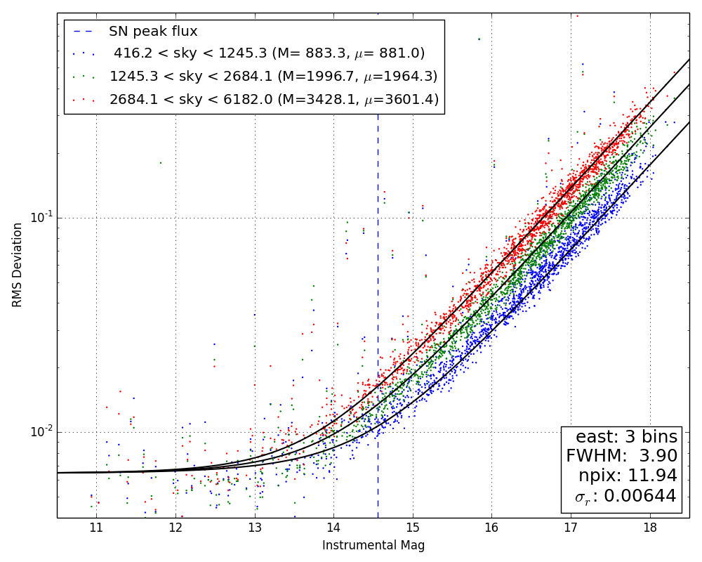
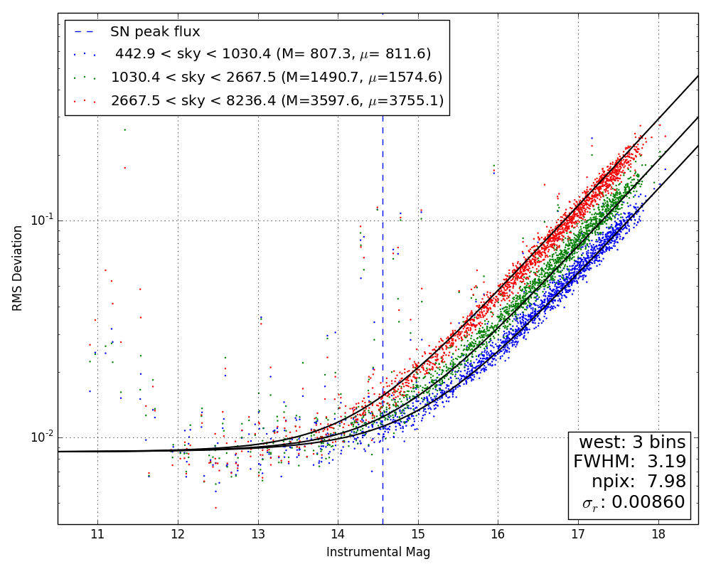
Figure 1.— KELT noise model for east data (left) and west data (right). We characterize our photometric uncertainties empirically using an ensemble of nearly 2000 stars in the vicinity of M82. We find that the KELT-North photometric performance (i.e., light curve scatter as a function of source brightness and sky level) is well approximated by a Poisson noise aperture photometry model with a constant $\sigma_{r}$ noise floor. Once the aperture area and noise floor are known, reliable photometric uncertainties may be calculated directly for any target.

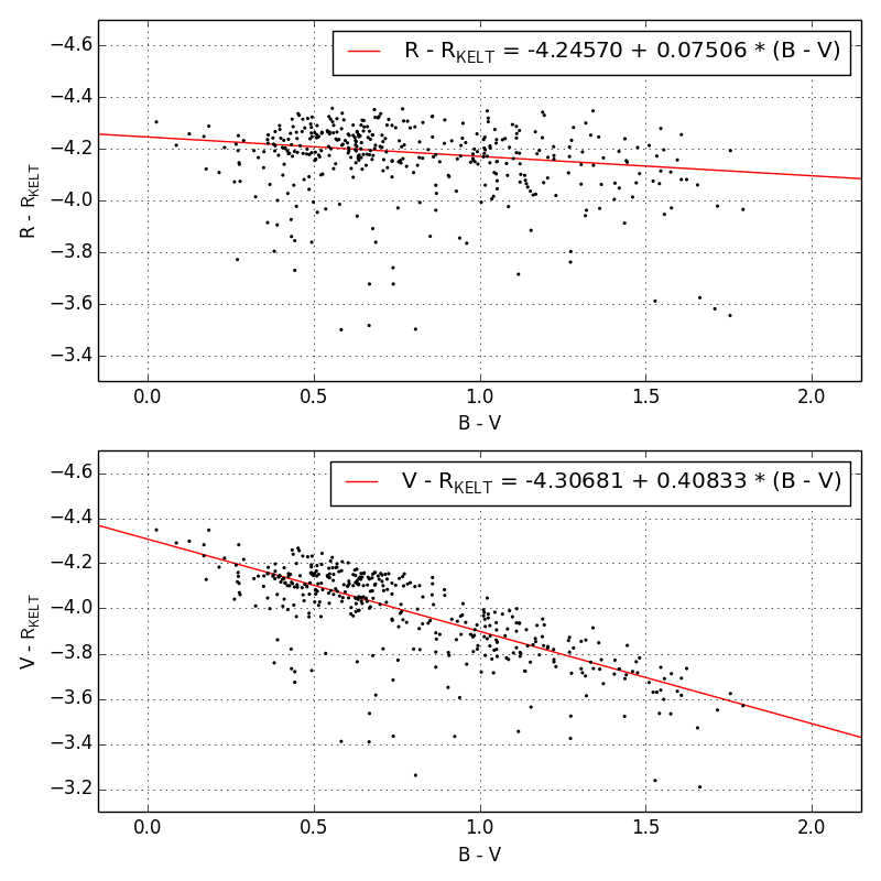
Figure 2.— Relationships between the KELT-North instrumental system and Johnson $V$ and $R$ magnitudes (see the text).

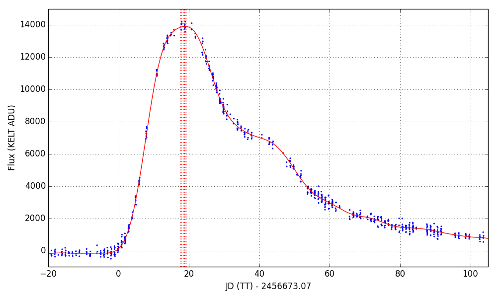
Figure 3.— KELT light curve of SN2014J (western data). Also shown is the range of peak time values (vertical lines) determined from best-fit empirical Fourier models (solid curve; see the text).

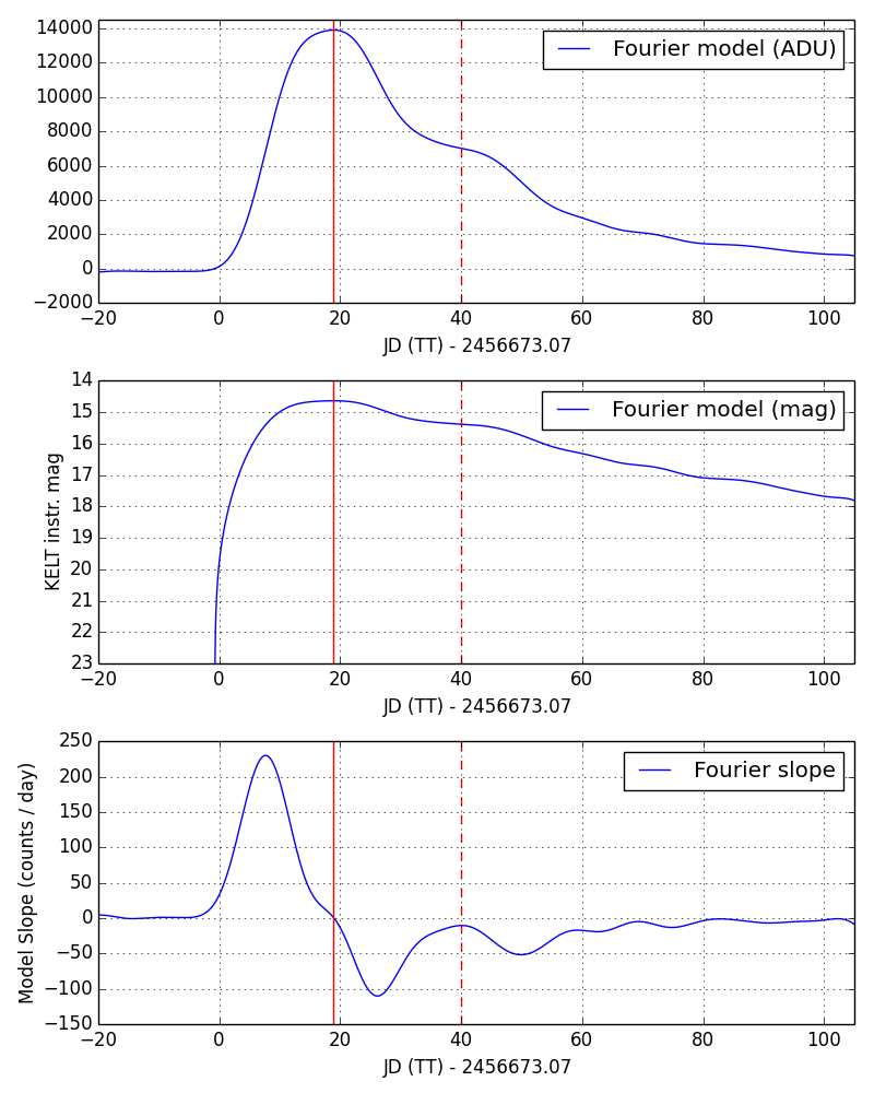
Figure 4.— Fourier representation of the light curve used to quantify the time of the secondary bump (see the text). (Top) Fourier representation of the light curve in flux units. (Middle) Same as top but in magnitudes. (Bottom) Slope in flux per unit time. In each panel, the time of primary peak is represented by the solid vertical line (corresponding to the peak in the top and middle panels), and the time of secondary bump is represented by the dashed vertical line (corresponding to the peak in the bottom panel).

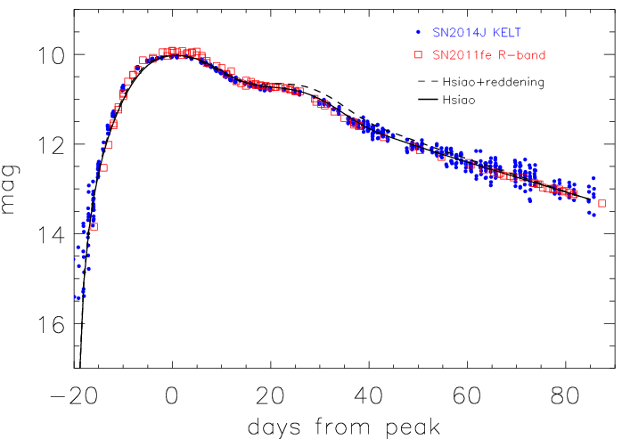
Figure 5.— The KELT-N light curve of SN 2014J (blue circles) is shown with the $R$-band data of SN 2011fe from (Munari et al., 2013) (red squares) and the synthetic model photometry (solid line) based on the empirical SNIa SED of Hsiao et al. (2007). The dashed line shows the expectation from the model SED once the effect of reddening is taken into account, i.e., including the effect of change of the effective wavelength. Note that the magnitudes from SN 2011fe are plotted exactly as tabulated in (Munari et al., 2013), i.e., without any adjustment for ”stretch” or in the vertical axis. The synthetic models based on Hsiao et al. (2007) have been shifted to match the peak brightness of SN 2014J.

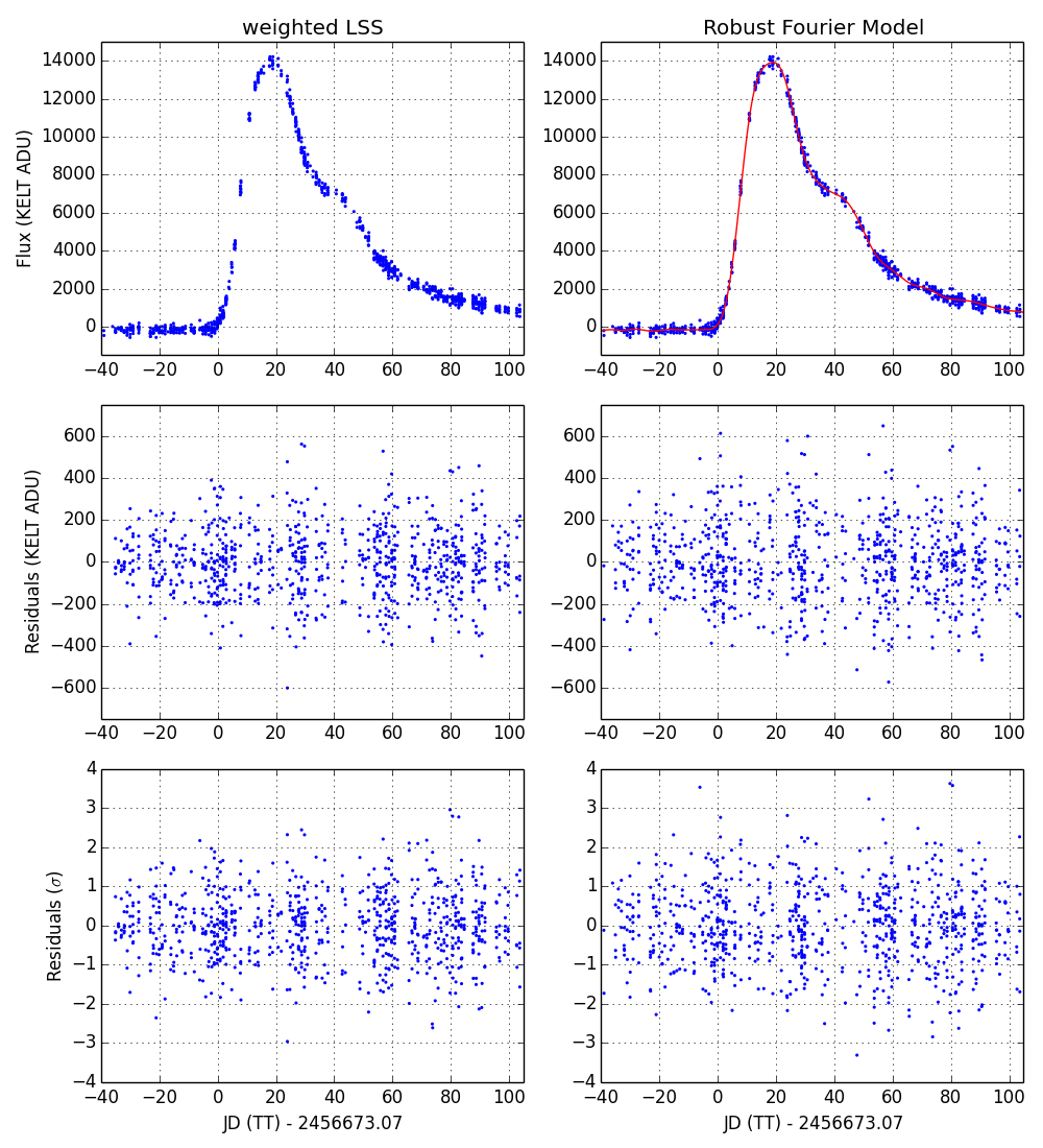
Figure 6.— Comparison of light curve intra-night scatter using two different fitting methods. Within each night with three or more data points, we fit a straight line to all data points. The top row depicts the SN2014J (west) light curve. The middle row shows the raw residuals in ADU (data points with the straight line fit subtracted). In the bottom row, residuals are divided by the uncertainties. Each column uses a different fitting method. Left uses weighted least-squares and right uses scatter about the empirical Fourier model fit. See the text.

References

- Alard (2000) Alard, C. 2000, A&AS, 144, 363
- Alard & Lupton (1998) Alard, C., & Lupton, R. H. 1998, ApJ, 503, 325
- Amanullah et al. (2014) Amanullah, R., Goobar, A., Johansson, J., et al. 2014, ApJ, 788, L21
- Bloom et al. (2012) Bloom, J. S., Kasen, D., Shen, K. J., et al. 2012, ApJ, 744, L17
- Brown et al. (2014) Brown, P. J., Smitka, M. T., Wang, L., et al. 2014, ArXiv e-prints, arXiv:1408.2381
- Cox (2000) Cox, A., 2000, Allen’s Astrophysical Quantities. Springer-Verlag, New York, p. 387
- Dalcanton et al. (2009) Dalcanton, J. J., Williams, B. F., Seth, A. C., et al. 2009, ApJS, 183, 67
- Fitzpatrick (1999) Fitzpatrick, E. L. 1999, PASP, 111, 63
- Foley et al. (2014) Foley, R. J., Fox, O., McCully, C., et al. 2014, ArXiv e-prints, arXiv:1405.3677
- Goobar et al. (2014a) Goobar, A., Kromer, M., Siverd, R., et al. 2014a, ArXiv e-prints, arXiv:1410.1363
- Goobar et al. (2014b) Goobar, A., Johansson, J., Amanullah, R., et al. 2014b, ApJ, 784, L12
- Høg et al. (2000) Høg, E., Fabricius, C., Makarov, V. V., et al. 2000, A&A, 355, L27
- Hsiao et al. (2007) Hsiao, E. Y., Conley, A., Howell, D. A., et al. 2007, ApJ, 663, 1187
- Huber (1981) Huber, P. J., 1981, Robust Statistics. John Wiley and Sons, Inc., New York
- Iben & Tutukov (1984) Iben, Jr., I., & Tutukov, A. V. 1984, ApJS, 54, 335
- Kasen (2010) Kasen, D. 2010, ApJ, 708, 1025
- Kelly et al. (2014) Kelly, P. L., Fox, O. D., Filippenko, A. V., et al. 2014, ApJ, 790, 3
- Lang et al. (2010) Lang, D., Hogg, D. W., Mierle, K., Blanton, M., & Roweis, S. 2010, AJ, 139, 1782
- Marion et al. (2014) Marion, G. H., Sand, D. J., Hsiao, E. Y., et al. 2014, ArXiv e-prints, arXiv:1405.3970
- Munari et al. (2013) Munari, U., Henden, A., Belligoli, R., et al. 2013, New Astr., 20, 30
- Nugent et al. (2011) Nugent, P. E., Sullivan, M., Cenko, S. B., et al. 2011, Nature, 480, 344
- Pepper et al. (2007) Pepper, J., et al. 2007, PASP, 119, 923
- Sen (1968) Sen, P. K. 1968, J. Am. Stat. Assoc., 63, 1379
- Siverd et al. (2012) Siverd, R. J., Beatty, T. G., Pepper, J., et al. 2012, ApJ, 761, 123
- Tutukov & Yungelson (1981) Tutukov, A. V., & Yungelson, L. R. 1981, Nauchnye Informatsii, 49, 3
- Webbink (1984) Webbink, R. F. 1984, ApJ, 277, 355
- Whelan & Iben (1973) Whelan, J., & Iben, Jr., I. 1973, ApJ, 186, 1007
- Zacharias et al. (2013) Zacharias, N., Finch, C. T., Girard, T. M., et al. 2013, AJ, 145, 44
- Zheng et al. (2014) Zheng, W., Shivvers, I., Filippenko, A., et al. 2014, ApJ, 783, L24