Distribution of Canonical Determinants in QCD

Abstract

The distribution of canonical determinants in QCD is determined by means of chiral perturbation theory. For a non-zero quark charge the canonical determinants take complex values. In the dilute pion gas approximation, we compute all moments of the magnitude of the canonical determinants, as well as the first nonvanishing moments of the real and imaginary parts. The non-trivial cancellation between the real and the imaginary parts of the canonical determinants is derived and the signal to noise ratio is discussed. The analytical distributions are compared to lattice data. The average density of the magnitude of the canonical determinants is determined as well and is shown to be given by a variant of the log-normal distribution.

I Introduction

QCD at finite baryon density and low temperatures is one of the least understood regions of the QCD phase diagram. The reason is that the baryon chemical potential introduces a sign problem which invalidates standard stochastic methods to evaluate the path integral for the QCD partition function. The source of the problem goes back to the fluctuations of the pions when the chemical potential exceeds half the pion mass. Then the value of the average fermion determinant is strongly suppressed with respect to the average of the magnitude of the fermion determinant (for reviews and additional details see deForcrand:2010ys ; Splittorff:2006vj ; Splittorff:2007zh ; Splittorff:2007ck ; Splittorff:2006fu ). One way to evade this problem might be to use the canonical ensemble haas ; deforcrand ; liu ; DG . This approach only requires the QCD partition function at imaginary chemical potential which can be calculated reliably by standard methods roberge ; alford ; mario ; philip . However, the extraction of the canonical partition function requires the evaluation of the Fourier transform

$$Z^{q}=\frac{1}{2\pi}\int_{-\pi}^{\pi}d\theta\;e^{-iq\theta}Z(\mu=i\theta T),$$ (1)

which in the thermodynamic limit, $q\to\infty$, leads to unmanageable cancellations. In lattice simulations, one can do better though. The fermion determinant at non-zero chemical potential is a polynomial in $\exp[\pm\mu/T]$,

$$Z(\mu)=\langle\sum_{q=-N}^{N}D_{q}\;e^{\mu q/T}\rangle,$$ (2)

so that $Z^{q}=\langle D_{q}\rangle$. Because this is a finite polynomial the Fourier coefficients can be determined exactly by means of a discrete Fourier transform. The computation of the average of the canonical determinants, however, remains a challenge. In this paper we show that this challenge depends crucially on the value of $q$. For small $q$ the signal to noise ratio is tractable while it becomes exponentially small with increasing $q$.

To address the signal to noise problem in the canonical approach we will evaluate the average magnitude of the canonical determinants to one-loop order in chiral perturbation theory and compare them to the average of the canonical determinants. This will give us information on the degree of cancellations that take place in evaluating the canonical partition function. The magnitude is obtained from the absolute value of the canonical determinants. This carries an isospin component which couples to the pions. On the contrary the charge dependence of the average of the canonical determinants themselves is not directly coupled to the pions. This difference leads to an exponentially small (in the charge) signal to noise ratio. We also obtain the full distribution of the absolute value of the canonical determinants and make comparisons with lattice results for the $q$-dependence of the canonical determinants.

The problems facing the canonical approach have also been emphasized in kaplan . Though the entire approach is different, the problems were traced back to the same source, namely that the average value of the baryon correlator is strongly suppressed with respect to the “noise” given by the absolute value squared correlator which at large distances is dominated by the contribution of the pions.

We start this paper with a discussion of canonical partition functions corresponding to non-zero isospin chemical potential (section 2). In section 3 we show that the same expressions give the magnitude of the canonical determinants at non-zero baryon number density. The relative size of the cancellations which take place in the evaluation of the canonical partition function is estimated in section 4 by modeling the nucleon contribution in terms of a resonance gas model. In section 5 we compare the $q$-dependence of the canonical partition functions with results from lattice QCD simulations. The full distribution of the magnitude of the canonical determinants is derived in section 6 and concluding remarks are made in section 7. Additional details are worked out in three appendices.

II Canonical partition functions for isospin charge

Before we turn to the distribution of the canonical determinants in QCD with non-zero quark charge it is useful to compute the canonical partition functions at fixed isospin number.

In oder to derive the canonical partition function with isospin charge we first recall the relation between the grand canonical partition function and the canonical partition function. For simplicity we consider two light flavors of mass $m$.

The two flavor QCD partition function at non-zero isospin chemical potential $\mu$ is given by

$$Z_{1+1^{*}}(\mu)=\langle{\det}(D+\mu\gamma_{0}+m)\det(D-\mu\gamma_{0}+m)\rangle,$$ (3)

where $D$ is the Dirac operator and the average is over the Yang-Mills action. This grand canonical partition function can be decomposed in terms of canonical partition functions as

$$Z_{1+1^{*}}(\mu)=\sum_{q=-\infty}^{\infty}e^{q\mu/T}Z_{1+1^{*}}^{q},$$ (4)

with

$$Z_{1+1^{*}}^{q}=\frac{1}{2\pi}\int_{-\pi}^{\pi}d\theta\ e^{-i\theta q}Z_{1+1^{*}}(\mu/T=i\theta).$$ (5)

We evaluate the canonical partition functions to one-loop order in chiral perturbation theory. At this order, the grand canonical partition function in the normal phase is given by Splittorff:2007ck

$$Z_{1+1^{*}}(\mu)=\langle{\det}(D+\mu\gamma_{0}+m)\det(D-\mu\gamma_{0}+m)\rangle\simeq e^{G_{0}|_{V=\infty}+g_{0}(\mu)},$$ (6)

where the $\mu$ dependence of the free energy resides entirely in the part (see STV )

$$g_{0}(\mu)=\frac{Vm_{\pi}^{2}T^{2}}{\pi^{2}}\sum_{n=1}^{\infty}\frac{K_{2}(\frac{m_{\pi}n}{T})}{n^{2}}\cosh(\frac{2\mu n}{T}).$$ (7)

The $\mu$ independent part, $G_{0}|_{V=\infty}$, will be suppressed throughout (the final results will be ratios where this contribution drops out). The corresponding canonical partition functions are given by the coefficients of $\exp(\mu q/T)$ in the expansion of the one-loop result for the $\mu$-dependent part of the grand canonical partition function in powers of $\exp(\mu/T)$

$$Z_{1+1^{*}}(\mu) = Z_{1+1^{*}}(\mu=0)\;\exp\left({\frac{Vm_{\pi}^{2}T^{2}}{\pi^{2}}\sum_{n=1}^{\infty}\frac{K_{2}(\frac{m_{\pi}n}{T})}{n^{2}}(\cosh(2\mu n/T)-1)}\right)$$ (8)

$$= \sum_{q}e^{q\mu/T}Z^{q}_{1+1^{*}}.$$

Using the asymptotic form of the Bessel function $K_{2}$ (which corresponds to the non-relativistic limit) we can make an estimate for the parameter domain where the terms with $n>1$ can be ignored. From the condition that the correction to the free energy density due to the $n=2$ term should be much less than the free energy density from the $n=1$ contribution we obtain

$$\frac{q(2mT)^{3/2}}{V_{3}}\ll\log\frac{V_{3}}{q(2mT)^{3/2}}.$$ (9)

Therefore for a dilute pion gas,

$$\frac{q}{V_{3}}\ll(2mT)^{3/2},$$ (10)

we can restrict ourselves to the $n=1$ term. This results in the canonical partition function

$$\frac{Z_{1+1^{*}}^{q}}{Z_{1+1^{*}}^{q=0}} = \frac{e^{-\omega}\int_{-\pi}^{\pi}\frac{d\theta}{2\pi}\ e^{-i\theta q}e^{\omega\cos(2\theta)}}{e^{-\omega}\int_{-\pi}^{\pi}\frac{d\theta}{2\pi}\ e^{\omega\cos(2\theta)}}$$ (11)

with $\omega$ defined by

$$\omega=\frac{V_{3}m_{\pi}^{2}T}{\pi^{2}}K_{2}(m_{\pi}/T).$$ (12)

For odd values of $q$ the canonical partition functions vanish. This is natural since the pions (in the convention used here) carry two units of isospin charge. For even $q$ the canonical integral is given by the modified Bessel function resulting in the ratio

$$\frac{Z_{1+1^{*}}^{q}}{Z_{1+1^{*}}^{q=0}} = \frac{I_{q/2}(\omega)}{I_{0}(\omega)},\qquad q\ {\rm even}.$$ (13)

Thus we have found that the distribution of the canonical partition functions over $q$ is described by the modified Bessel functions . For $m_{\pi}/T\gg 1$ we can also replace $K_{2}$ by its asymptotic form resulting in

$$\frac{Z_{1+1^{*}}^{q}}{Z_{1+1^{*}}^{q=0}} = \frac{I_{q/2}\big{(}\frac{V_{3}m_{\pi}^{3/2}T^{3/2}}{\sqrt{2\pi^{3}}}e^{-m_{\pi}/T}\big{)}}{I_{0}\big{(}\frac{V_{3}m_{\pi}^{3/2}T^{3/2}}{\sqrt{2\pi^{3}}}e^{-m_{\pi}/T}\big{)}},\qquad q\ {\rm even}.$$ (14)

The chemical potential corresponding to the canonical partition function is worked out in Appendix A.

Finally, it is instructive to sum over $q$ to obtain the grand canonical partition function

$$Z_{1+1^{*}}(\mu) = \sum_{q=-\infty}^{\infty}e^{q\mu/T}Z_{1+1^{*}}^{q}$$

$$= Z_{1+1^{*}}(\mu=0)\sum_{j=-\infty}^{\infty}e^{2j\mu/T-\omega}I_{j}\Big{(}\frac{Vm_{\pi}^{3/2}T^{5/2}}{\sqrt{2}\pi^{3/2}}e^{-m_{\pi}/T}\Big{)}$$

$$= Z_{1+1^{*}}(\mu=0)\;\exp\left(\frac{Vm_{\pi}^{3/2}T^{5/2}}{2\sqrt{2}\pi^{3/2}}(e^{(2\mu-m_{\pi})/T}+e^{(-2\mu-m_{\pi})/T}-2e^{-m_{\pi}/T})\right),$$

which, as it should, brings us back to our starting point.

As we shall see below, the computation of the distribution of the canonical determinants at non-zero quark charge has many analogies to the above computation of the canonical partition functions as a function of isospin charge. Let us therefore briefly discuss the overall structure of these computations: For the Fourier transform (5) we need the partition function at non-zero imaginary isospin chemical potential. For real isospin chemical potential less than $m_{\pi}/2$ the partition function is in the normal phase and the expression (6) is the 1-loop result from chiral perturbation theory for this phase. This leading order expression for small real isospin chemical potential is also the leading contribution at imaginary isospin chemical potential. For a real isospin chemical potential larger than $m_{\pi}/2$ the partition function is in a pion condensed phase. At imaginary isospin chemical potential this implies that there is a sub-leading saddle point, which is not taken into account above. The analytic form of this contribution is worked out using mean field chiral perturbation theory in Appendix C.

III The canonical determinants at non-zero quark charge

Let us now turn to quark chemical potential. Since the pions have zero quark charge we obviously have

$$Z^{q\neq 0}=0$$ (16)

when evaluated in CPT. However, the fermion determinant at non-zero chemical potential can be decomposed into canonical determinants before averaging over the gauge fields

$$\det(D+m+\mu\gamma_{0})=\sum_{q}e^{\mu q/T}D_{q},$$ (17)

with

$$D_{q}=\frac{1}{2\pi}\int_{-\pi}^{\pi}d\theta e^{-i\theta q}\det(D+m+i\theta T\gamma_{0}).$$ (18)

Note that $D_{q=0}$ is real.

Although pions do not have baryon charge, they contribute to the magnitude of $D_{q}$,

$$\langle|D_{q}|^{2}\rangle = \int\frac{d\theta_{1}\ d\theta_{2}}{(2\pi)^{2}}\ e^{-i(\theta_{1}-\theta_{2})q}\;\langle\det(D+m+i\theta_{1}T\gamma_{0})\det(-D+m-i\theta_{2}T\gamma_{0})\rangle$$ (19)

$$= \int\frac{d\theta_{1}\ d\theta_{2}}{(2\pi)^{2}}\ e^{-i(\theta_{1}-\theta_{2})q}\;\langle\det(D+m+i\theta_{1}T\gamma_{0})\det(D+m+i\theta_{2}T\gamma_{0})\rangle.$$

The reason is that

$$\langle\det(D+m+i\theta_{1}T\gamma_{0})\det(D+m+i\theta_{2}T\gamma_{0})\rangle$$ (20)

is the partition function at non-zero imaginary quark, $i(\theta_{1}+\theta_{2})T$, and isospin, $i(\theta_{1}-\theta_{2})T$, chemical potential. The double Fourier transform in (19) singles out the contribution with isospin charge $q$ and zero baryon charge. To one-loop order in chiral perturbation theory it is given by

$$\frac{\langle\det(D+m+i\theta_{1}T\gamma_{0})\det(D+m+i\theta_{2}T\gamma_{0})\rangle}{\langle\det(D+m)^{2}\rangle}$$ (21)

$$= \frac{\exp\Big{(}\frac{Vm_{\pi}^{2}T^{2}}{\pi^{2}}\sum_{n=1}^{\infty}\frac{K_{2}(\frac{m_{\pi}n}{T})}{n^{2}}\cos((\theta_{1}-\theta_{2})n)\Big{)}}{\exp\Big{(}\frac{Vm_{\pi}^{2}T^{2}}{\pi^{2}}\sum_{n=1}^{\infty}\frac{K_{2}(\frac{m_{\pi}n}{T})}{n^{2}}\Big{)}}.$$

For $m_{\pi}/T\gg 1$ when the inequality (10) is satisfied, the average $\langle|D_{q}|^{2}\rangle$ normalized to the $q=0$ expression simplifies to

$$\frac{\langle|D_{q}|^{2}\rangle}{\langle|D_{q=0}|^{2}\rangle} = \frac{\int d\theta_{-}\ e^{-iq\theta_{-}}e^{\frac{Vm_{\pi}^{2}T^{2}}{\pi^{2}}K_{2}(\frac{m_{\pi}}{T})\cos(\theta_{-})}}{\int d\theta_{-}\ e^{\frac{Vm_{\pi}^{2}T^{2}}{\pi^{2}}K_{2}(\frac{m_{\pi}}{T})\cos(\theta_{-})}}$$ (22)

$$= \frac{I_{q}(\omega)}{I_{q=0}(\omega)}.$$

This main result is compared to lattice data in section V.

In order to address the cancellations in the average of the canonical determinant we now evaluate also $\langle D_{q}^{2}\rangle$. This computation follows the same lines as above and instead of (22) we obtain

$$\langle D_{q}^{2}\rangle = \int\frac{d\theta_{1}\ d\theta_{2}}{(2\pi)^{2}}\ e^{-i(\theta_{1}+\theta_{2})q}\;\langle\det(D+m+i\theta_{1}T\gamma_{0})\det(D+m+i\theta_{2}T\gamma_{0})\rangle.$$ (23)

Using the one-loop result we obtain for $m_{\pi}/T\gg 1$,

$$\frac{\langle D_{q}^{2}\rangle}{\langle D_{q=0}^{2}\rangle} = \frac{\int d\theta_{+}d\theta_{-}\ e^{-iq\theta_{+}}e^{\frac{Vm_{\pi}^{2}T^{2}}{\pi^{2}}K_{2}(\frac{m_{\pi}}{T})\cos(\theta_{-})}}{\int d\theta_{+}d\theta_{-}\ e^{\frac{Vm_{\pi}^{2}T^{2}}{\pi^{2}}K_{2}(\frac{m_{\pi}}{T})\cos(\theta_{-})}}$$ (24)

$$= \delta_{q0},$$

as expected, since the double Fourier transform in (23) singles out the contribution with quark charge $q$ and pions have zero baryon number.

In order to understand better how $\langle D_{q}^{2}\rangle=0$ for $q\neq 0$ is formed, first note that we have $\langle{D_{q}^{*}}^{2}\rangle=\langle D_{q}^{2}\rangle$, which can be rewritten as

$$\langle{\rm Re}[D_{q}]{\rm Im}[D_{q}]\rangle=0.$$ (25)

Now, let us express the expectation value of $D_{q}^{2}$ in terms of the expectation value of its real and imaginary parts

$$\langle D_{q}^{2}\rangle=\frac{1}{4}\langle(D_{q}+D_{q}^{*})^{2}\rangle+\frac{1}{4}\langle(D_{q}-D_{q}^{*})^{2}\rangle.$$ (26)

Next note that both the square of the real part and the square of the imaginary part contain $|D_{q}|^{2}$:

$$\left\langle(D_{q}^{*}\pm D_{q})^{2}\right\rangle=2\left\langle D_{q}^{2}\pm|D_{q}|^{2}\right\rangle.$$ (27)

Therefore, the canonical determinants with non-zero $q$ have equal variance in the real and the imaginary direction of the complex plane (when evaluated within chiral perturbation theory). These contributions cancel in the evaluation of $\left\langle D_{q}^{2}\right\rangle$.

We can also calculate the average value of $|D_{q}|^{2}$ from the mean field expression for the free energy in the condensed phase. The calculation proceeds along the steps of Appendix C and one obtains the result

$$\frac{\langle|D_{q}|^{2}\rangle}{\langle|D_{q=0}|^{2}\rangle}=e^{-q^{2}/8V_{4}F^{2}T^{2}-|q|m_{\pi}/T}\;.$$ (28)

IV Signal to noise ratio

In the previous section we have seen that to one-loop order in chiral perturbation theory $\langle D_{q}^{2}\rangle=0$ for $q\neq 0$. The reason is that in this limit the partition function does not contain any baryons. The effect of nucleons can be taken into account schematically by means of the Hadron Resonance Gas model for $T\ll m_{N}$ resulting in the ratio of the two-flavor partition functions

$$\frac{Z_{q}(m_{N})}{Z_{q=0}(m_{N})}\equiv\frac{\langle D_{q}^{2}\rangle}{\langle D_{q=0}^{2}\rangle}=\frac{I_{q/3}(\omega_{N})}{I_{q=0}(\omega_{N})},$$ (29)

where

$$\omega_{N}=\frac{Vm_{N}^{2}T^{2}}{\pi^{2}}K_{2}(m_{N}/T),$$ (30)

with $m_{N}$ the nucleon mass . Therefore the ’signal to noise’ ratio of the average canonical determinants is given by (note that $D_{q=0}$ is real and hence that $D_{q=0}^{2}=|D_{q=0}|^{2}$)

$$\frac{\langle D_{q}^{2}\rangle}{\langle|D_{q}|^{2}\rangle}=\frac{I_{q/3}(\omega_{N})}{I_{q/2}(\omega)}.$$ (31)

For large $q$ the ratio $I_{q/3}(Vx)/I_{q/2}(Vy)$ goes as $(x^{1/3}/y^{1/2})^{q}$. Using this we find in the dilute limit

$$\frac{\langle D_{q}^{2}\rangle}{\langle|D_{q}|^{2}\rangle}\simeq e^{-q(m_{N}/3-m_{\pi}/2)/T}.$$ (32)

Note that the factors of $V$ cancels. Since $m_{N}/3>m_{\pi}/2$ we conclude that at fixed baryon density the signal to noise ratio becomes exponentially small in the thermodynamic limit.

V Lattice Results for Canonical Determinants

The distribution of the canonical determinants has been measured in lattice QCD in DG ; BDGLL ; AW . In this section we make a first qualitative comparison of the analytical prediction for the $q$ dependence of the average magnitude of the canonical determinants, Eq. (22), to lattice data.

The results we present are for ensembles of $N_{f}=2$ Wilson fermions on $12^{3}\times 6$ lattices generated with the MILC code MILC . A hopping parameter of $\kappa=0.162$ is used and we show results for $\beta=5.025$ and $\beta=5.325$, which corresponds to temperatures of $T=100MeV$ and $T=140$ MeV. The lattice spacing was determined from the Wilson flow and the pion masses are $m_{\pi}\sim 900$ MeV. The errors we show are statistical errors determined with the jackknife method.

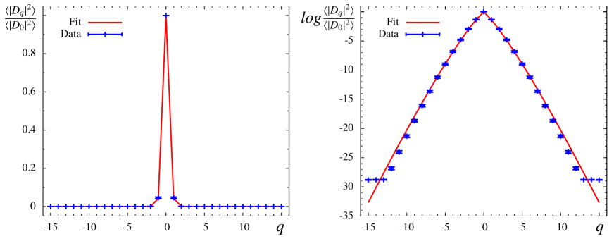
Figure 1: Left: Lattice results for $\langle|D_{q}|^{2}\rangle/\langle|D_{0}|^{2}\rangle$ (points) at $T=100$ MeV together with a fit of $I_{q}(\omega)/I_{0}(\omega)$ (solid red curve) as a function of $q$ (left). Right: Same data after taking the logarithm, i.e. $\log\left(\langle|D_{q}|^{2}\rangle/\langle|D_{0}|^{2}\rangle\right)$ as a function of $q$. The fit includes the range $-6\leq q\leq 6$ and the fitted value is $\omega=0.085$ (reduced $\chi^{2}\simeq 0.4$). The $q$ independence of the data points for $|q|\geq 13$ is due to insufficient numerical precision.

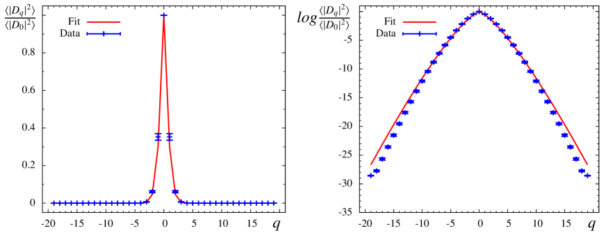
Figure 2: As in figure 1 but now for $T=140$ MeV: Lattice results for $\langle|D_{q}|^{2}\rangle/\langle|D_{0}|^{2}\rangle$ (left) and for $\log(\langle|D_{q}|^{2}\rangle/\langle|D_{0}|^{2}\rangle)$ (right). Again the fit is based on the lower range of $q$, here $-9\leq q\leq 9$ ($\omega=0.628$ reduced $\chi^{2}\simeq 3.6$), where the analytical expression is expected to hold best.

We have computed $\langle|D_{q}|^{2}\rangle/\langle|D_{0}|^{2}\rangle$ on these lattices and have used the argument, $\omega$, of the Bessel $I_{q}$ functions in Eq. (22) as a fitting parameter. In Fig. 1 we show the results for a temperature of $T=100$ MeV. The data for $|q|\geq 13$ are not to be considered (the accuracy of the Fourier transform used does not allow to compute canonical determinants for $|q|\geq 13$). We observe that the fit works well over 20 orders of magnitude. We have used the data in the range $|q|\leq 6$ for the fit which returns the value $\omega=0.085$, with a reduced $\chi^{2}\simeq 0.4$.

Despite the higher temperature the fit for $T=140$ MeV shown in Fig. 2 is almost as good. The fitted values of $\omega$ in this case is $\omega=0.628$ with a reduced $\chi^{2}$ of $3.6$.

For larger values of $q$ we find significant deviations between the lattice results and the analytical fits. This could be due to the larger $n$ contributions in the ratio of the canonical determinants

$$\frac{\langle|D_{q}|^{2}\rangle}{\langle|D_{q=0}|^{2}\rangle} = \frac{\int\frac{d\theta_{-}}{2\pi}\ e^{-iq\theta_{-}}e^{\frac{Vm_{\pi}^{2}T^{2}}{\pi^{2}}\sum_{n=1}^{\infty}\frac{K_{2}(\frac{m_{\pi}n}{T})}{n^{2}}\cos(n\theta_{-})}}{\int\frac{d\theta_{-}}{2\pi}\ e^{\frac{Vm_{\pi}^{2}T^{2}}{\pi^{2}}\sum_{n=1}^{\infty}\frac{K_{2}(\frac{m_{\pi}n}{T})}{n^{2}}\cos(n\theta_{-})}}.$$ (33)

Numerically it is no problem to keep more terms in this sum. In Fig. 3 we compare the $I_{q}/I_{0}$ distribution (obtained keeping only the $n=1$ term) to the distribution we get keeping the $n\leq 2$ terms and all terms. As expected the higher $n$ terms affect the larger $q$ values more. The effect is of the same magnitude as the deviation of the lattice data from the analytical prediction but the sign is opposite.

Because of the rather large pion mass in the present simulation, further lattice studies are required in order to quantify the test of the analytic expression.

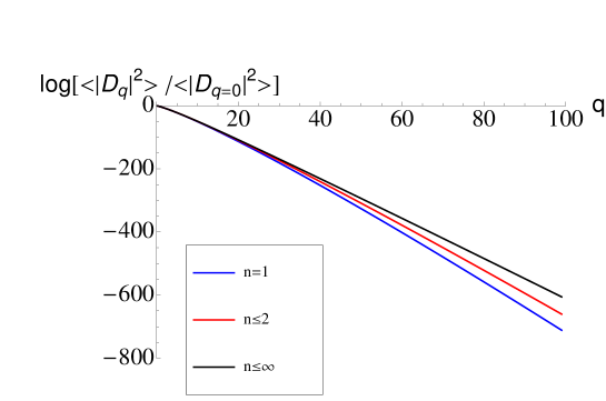
Figure 3: The curves show $\log[\langle|D_{q}|^{2}\rangle/\langle|D_{q=0}|^{2}\rangle$ for $V_{3}m_{\pi}^{3}=2000$ and $T/m_{\pi}=1/6$ (i.e. $\omega=0.56/\pi^{2}$), for $n=1$ (blue), $n\leq 2$ (red) and with all values of $n$ included (black).

VI Full Distribution of the Magnitude of the Canonical Determinants

In this section we will evaluate the average of all moments of $|D_{q}|^{2}$ in the limit of a dilute pion gas and obtain an analytical expression for the density $\rho_{q}(x)$. The probability density of the magnitude of the determinants is given by

$$\rho_{q}(x) = \langle\delta(|D_{q}|^{2}-x)\rangle$$ (34)

$$= \Big{\langle}\frac{1}{2\pi}\int_{-\infty}^{\infty}dse^{-is(|D_{q}|^{2}-x)}\Big{\rangle}$$

$$= \frac{1}{2\pi}\int_{-\infty}^{\infty}ds\sum_{p=0}^{\infty}\frac{\langle(-is|D_{q}|^{2})^{p}\rangle}{p!}e^{isx}.$$

Let us first consider the $p$-th moment of the absolute value squared of the fermion determinant to one loop order in chiral perturbation theory. The partition function is the same as for the theory for $2p$ flavors and, to one loop order, each flavor contributes GL

$$-\frac{1}{2}g_{0}(m_{\pi}^{2},T,L)$$ (35)

to the free energy. For the $2p$ moment we thus find for vanishing isospin chemical potential

$$\langle{\det}^{2p}(D+m)\rangle=Ce^{\frac{1}{2}(4p^{2}-1)g_{0}(m_{\pi},T)},$$ (36)

which are the moments of a log-normal distribution.

For convenience we use in this section a slightly different normalization of $D_{q}$ which includes the contribution of the neutral pions and denote the canonical determinants by $\tilde{D}_{q}$. In this normalization we obtain the moments

$$\langle|\tilde{D}_{q}|^{2p}\rangle = e^{(p-\frac{1}{2})\omega}\int\prod_{k=1}^{p}\frac{d\theta_{k}\ d\phi_{k}}{(2\pi)^{2}}$$

$$\times\prod_{k=1}^{p}e^{-i(\theta_{k}-\phi_{k})q}e^{\frac{Vm_{\pi}^{2}T^{2}}{\pi^{2}}K_{2}(\frac{m_{\pi}}{T})[\sum_{k<l}\cos(\theta_{k}-\theta_{l})+\cos(\phi_{k}-\phi_{l})+\sum_{k,l}\cos(\theta_{k}-\phi_{l})]}.$$

where the first exponent is the contribution due to the $2p-1$ neutral pions. The second factor in the exponent can be rewritten as

$$\sum_{k<l}[\cos(\theta_{k}-\theta_{l})+\cos(\phi_{k}-\phi_{l})]+\sum_{k,l}\cos(\theta_{k}-\phi_{l})$$

$$=\frac{1}{2}(\sum_{k=1}^{p}\cos\theta_{k}+\sum_{k=1}^{p}\cos\phi_{l})^{2}+\frac{1}{2}(\sum_{k=1}^{p}\sin\theta_{k}+\sum_{k=1}^{p}\sin\phi_{l})^{2}-p.$$ (38)

The squares can be linearized by a Hubbard-Stratonovich transformation. This results in

$$\langle|\tilde{D}_{q}|^{2p}\rangle = \int\frac{d\alpha d\beta}{2\pi}e^{-\alpha^{2}/2-\beta^{2}/2-\omega/2}\int\prod_{k=1}^{2p}\frac{d\phi_{k}d\theta_{k}}{2\pi^{2}}e^{iq(\phi_{1}+\cdots+\phi_{p})}e^{-iq(\theta_{1}+\cdots+\theta_{p})}$$ (39)

$$\times e^{-\omega^{1/2}\alpha(\sum_{k=1}^{p}\cos\theta_{k}+\sum_{k=1}^{p}\cos\phi_{l})-\omega^{1/2}\beta(\sum_{k=1}^{p}\sin\theta_{k}+\sum_{k=1}^{p}\sin\phi_{l})}.$$

The sines and cosines can be added as

$$\alpha\cos\phi+\beta\sin\phi=\sqrt{\alpha^{2}+\beta^{2}}\cos(\phi+\phi_{0}),$$ (40)

where

$$\cos\phi_{0}=\frac{\alpha}{\sqrt{\alpha^{2}+\beta^{2}}},$$ (41)

and the same for the $\theta$-variable. After shifting $\phi$ and $\theta$ by $-\phi_{0}$ we obtain

$$\langle|D_{q}|^{2p}\rangle = \int\frac{d\alpha d\beta}{2\pi}e^{-\alpha^{2}/2-\beta^{2}/2-\omega/2}$$ (42)

$$\times\left[\int\frac{d\phi}{2\pi}e^{iq\phi-\omega^{1/2}\sqrt{\alpha^{2}+\beta^{2}}\cos\phi}\right]^{p}\left[\int\frac{d\theta}{2\pi}e^{-iq\theta-\omega^{1/2}\sqrt{\alpha^{2}+\beta^{2}}\cos\theta}\right]^{p}$$

$$= e^{-\omega/2}\int_{0}^{\infty}rdre^{-r^{2}/2}\left[\int d\phi e^{iq\phi-\omega^{1/2}r\cos\phi}\right]^{2p}$$

$$= e^{-\omega/2}\int_{0}^{\infty}rdre^{-r^{2}/2}[I_{q}(\omega^{1/2}r)]^{2p}.$$

For $p=1$ the integral can be evaluated analytically

$$e^{-\omega/2}\int_{0}^{\infty}rdre^{-r^{2}/2}[I_{q}(\omega^{1/2}r)]^{2}=e^{\omega/2}I_{q}(\omega).$$ (43)

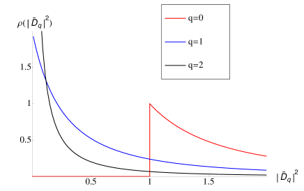
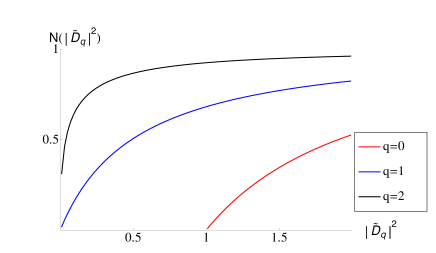
Figure 4: The distribution (left) and the cumulative distribution (right) of the absolute value squared for the canonical determinants $\tilde{D}_{q}$. Results are given for $q=0$, $q=1$ and $q=2$.

The normalized moments are given by

$$\frac{\langle|\tilde{D}_{q}|^{2p}\rangle}{\langle|\tilde{D}_{q}|^{0}\rangle} = \int_{0}^{\infty}rdre^{-r^{2}/2}[I_{q}(\omega^{1/2}r)]^{2p}.$$ (44)

The sum over $p$ in Eq. (34) can be evaluated analytically after inserting the expression (44) for the moments. This results in the average density

$$\rho_{q}(x) = \frac{1}{2\pi}\int_{-\infty}^{\infty}ds\int_{0}^{\infty}rdre^{-r^{2}/2}e^{-is(I_{q}(\omega^{1/2}r))^{2}}e^{isx}$$ (45)

$$= \int_{0}^{\infty}rdre^{-r^{2}/2}\delta(I_{q}(\omega^{1/2}r))^{2}-x)$$

$$= \left.\frac{ye^{-y^{2}/2\omega}}{2\omega I_{q}^{\prime}(y)I_{q}(y)}\right|_{I_{q}(y)=\sqrt{x}}.$$

This can also be written as

$$P\Big{[}[I_{q}^{2}]^{-1}[|\tilde{D}_{q}|^{2}]\in[x,x+dx]\Big{]}=\frac{x}{\omega}e^{-x^{2}/2\omega}dx,$$ (46)

with $[I_{q}^{2}]^{-1}$ the inverse of the function $x\to I_{q}^{2}(x)$. This is a variant of a log-normal distribution which can be seen by keeping only the exponential factor in the asymptotic expansion of the Bessel functions. For large determinants we thus find

$$P\Big{[}\log|\tilde{D}_{q}|\in[x,x+dx]\Big{]}\sim\frac{x}{\omega}e^{-x^{2}/2\omega}dx.$$ (47)

Another useful quantity is the cumulative distribution of the canonical determinants. It is given by

$$N_{q}(y) = \int_{0}^{y}\rho_{q}(y)dy$$ (48)

$$= \frac{1}{\omega}\int_{0}^{\bar{r}(y)}rdre^{-r^{2}/2\omega}$$

$$= 1-e^{-\bar{r}^{2}(y)/2\omega}$$

with $I_{q}(\bar{r}(y))=\sqrt{y}$. For large $q$ we have that $I_{q}(x)\sim(x/2)^{q}/q!$ so that $\bar{r}\sim 2qy^{1/2q}/e$ resulting in the cumulative distribution

$$N(y)\sim 1-e^{-2q^{2}y^{1/q}/\omega e^{2}}.$$ (49)

VII Conclusions

For a fixed non-zero quark charge the canonical determinants in QCD take complex values. The average of these canonical determinants is the corresponding canonical partition function, which is a real and positive number. To address the cancellations which take place in forming the canonical partition functions we have computed the distribution of the canonical determinants by means of chiral perturbation theory. In the limit of a dilute pion gas, the result simplifies to an expression in terms of modified Bessel functions. There are strong cancellations between the real and imaginary parts of the canonical determinants which lead to an exponential suppression, $\exp(-q(m_{N}/3-m_{\pi}/2))$, with respect to the average magnitude. The magnitude is strongly fluctuating as well with a distribution that in the low-temperature limit is given by a variant of the log-normal distribution. Moreover, we have evaluated the canonical partition functions at non-zero isospin density.

Our results were obtained by means of chiral perturbation theory in the dilute limit, and as demonstrated the analytical form agrees qualitatively with lattice QCD results over 20 orders of magnitude. The only caveat is that we used the arguments of the Bessel functions as a fitting parameter and that the value of the pion mass is outside the domain where chiral perturbation theory can be applied reliably. Consistent with the evaluation of the absolute value squared of the determinants in the dilute limit, the agreement is better for small $q$. Further lattice studies with lighter quarks are needed for a full quantitative test of the analytic results. For such a test additional terms from the low temperature expansion should be included for the larger $q$ values.

We have also determined the contribution to the canonical determinants from the mean field saddle point corresponding to the Bose condensed phase. We find an exponential suppression for small $q$ which turns into a Gaussian tail for large $q$. This effect becomes more relevant for larger values of $q$.

It would be most interesting to determine the distribution of the canonical determinants in improved lattice simulations with light quarks. This would allow for a quantitative test of the analytical predictions and lead to a better understanding of the large $q$ behavior of the canonical determinants.

Acknowledgments: This work was supported by U.S. DOE Grant No. DE-FG-88ER40388 (JV), the Austrian Science Fund FWF Grant Nr. I 1452-N27 (CG), FWF DK W1203 “Hadrons in Vacuum, Nuclei and Stars” (H-PS), The U.S. National Science Foundation CAREER grant PHY-1151648 and the Sapere Aude program of The Danish Council for Independent Research (KS).

Appendix A Isospin chemical potential from the canonical partition functions

The isospin chemical potential corresponding to the canonical partition function (13) is given by

$$\mu_{I}(T,n_{I}) = \frac{1}{2}(-T\log Z_{q+2}+T\log Z_{q})$$ (50)

$$= -\frac{T}{2}\log\frac{I_{(q+2)/2}(\omega)}{I_{q/2}(\omega)}.$$

In the thermodynamic limit the chemical potential at fixed isospin density is given by

$$\mu_{I}(T,n_{I}) = -\frac{T}{2}\lim_{q\to\infty}\log\frac{I_{(q+2)/2}(q\tilde{\omega})}{I_{q/2}(q\tilde{\omega})}$$ (51)

with

$$\tilde{\omega}=\frac{\omega}{q}=\frac{m_{\pi}^{2}T}{n_{I}\pi^{2}}K_{2}(m_{\pi}/T),$$ (52)

and $n_{I}$ is the isospin charge density

$$n_{I}=\frac{q}{V_{3}}.$$ (53)

For large $q$ we can use the uniform approximation for modified Bessel functions

$$I_{q}(qz)\sim\frac{1}{\sqrt{2\pi q}}\frac{e^{q\eta}}{(1+z^{2})^{1/4}}$$ (54)

with

$$\eta=\sqrt{1+z^{2}}+\log(z/2)-\log(\frac{1}{2}+\frac{1}{2}\sqrt{1+z^{2}}).$$ (55)

In the low temperature limit, the argument of the modified Bessel functions is small so that

$$\eta\sim 1+\frac{1}{4}z^{2}+\log(z/2),$$ (56)

and

$$I_{\nu}(\nu z)\sim\frac{(z/2)^{\nu}}{\sqrt{2\pi\nu}}e^{\nu(1+\frac{1}{4}z^{2})-\frac{1}{4}z^{2}}.$$ (57)

For large $q$ and low temperatures we thus have

$$I_{q/2}(q\tilde{\omega}) \sim \frac{\tilde{\omega}^{q/2}}{\sqrt{\pi q}}e^{q/2+\tilde{\omega}^{2}(q/2-1)},$$

$$I_{(q+2)/2}(q\tilde{\omega}) \sim \frac{(\tilde{\omega}q/(q+2))^{(q+2)/2}}{\sqrt{\pi(q+2)}}e^{(q+2)/2+\tilde{\omega}^{2}q^{3}/2(q+1)^{2}}.$$ (58)

In the large $q$ limit $I_{(q+2)/2}(q\tilde{\omega})$ simplifies to

$$I_{(q+2)/2}(q\tilde{\omega}) \sim \frac{\tilde{\omega}^{q/2}}{\sqrt{\pi q}}e^{(q+2)/2+\tilde{\omega}^{2}q/2}.$$ (59)

This results in the ratio

$$\frac{I_{(q+2)/2}(q\tilde{\omega})}{I_{q/2}(q\tilde{\omega})}\sim\tilde{\omega}e^{\tilde{\omega}^{2}/2}.$$ (60)

For $\tilde{\omega}\ll 1$ we obtain

$$\frac{I_{(q+2)/2}(q\tilde{\omega})}{I_{q/2}(q\tilde{\omega})}\sim\tilde{\omega}.$$ (61)

This results in the chemical potential

$$\mu_{I}(T,n_{I}) \approx -\frac{T}{2}\log\tilde{\omega}$$ (62)

$$= \frac{m_{\pi}}{2}-\frac{T}{2}\log\left[\frac{m_{\pi}^{3/2}T^{3/2}}{n_{I}\sqrt{2\pi^{3}}}\right].$$

In order to occupy the zero momentum states we need that $\mu>m_{\pi}/2$. The critical temperature for the formation of a pion condensate is thus given by the relation $\mu_{I}(T_{c},n_{I})=m_{\pi}/2$. In the low temperature limit the critical temperature in the $n=1$ approximation is thus given by

$$T_{c}=2^{1/3}\pi\frac{n_{I}^{2/3}}{m_{\pi}},$$ (63)

which up to the proportionality constant agrees with the result first obtained by Einstein einstein (See Appendix B). It should be noted that for $(2mT)^{3/2}/n_{I}\sim O(1)$ the sum over $n$ in Eq. (8) cannot be truncated to its first term. A calculation of the critical temperature that includes all terms is given in Appendix B.

Appendix B Critical Temperature for an Ideal Bose Gas

In this Appendix we determine the critical temperature for a noninteracting Bose gas (see for example einstein ; vosk ) and explain that the low temperature approximation gives the correct scaling behavior but does not reproduce the proportionality constant.

For density $n_{I}$, the critical temperature is given by the condition

$$\frac{1}{2}n_{I}=\left.\int\frac{d^{3}p}{(2\pi)^{3}}\frac{1}{e^{\beta(\sqrt{p^{2}+m^{2}_{\pi}}-2\mu)}-1}\right|_{\mu=m_{\pi}/2}.$$ (64)

In the nonrelativistic approximation, this simplifies to

$$\frac{1}{2}n_{I} = \frac{1}{2\pi^{2}}\int p^{2}dp\frac{1}{e^{\beta p^{2}/2m}-1}$$ (65)

$$= \frac{1}{2\pi^{2}}(2mT)^{3/2}\int x^{2}dx\frac{1}{e^{x^{2}}-1}.$$

The integral can be evaluated as

$$\int x^{2}dx\frac{1}{e^{x^{2}}-1}=\frac{1}{4}\sqrt{\pi}\zeta(3/2)\approx 1.15758.$$ (66)

The numerical constant obtained this way differs from the constant in (63). However, if we make the same approximation as in the derivation of Eq. (63), namely replacing the integral by

$$\int_{0}^{\infty}dx\frac{x^{2}}{e^{x^{2}}-1}\to\int_{0}^{\infty}dxx^{2}e^{-x^{2}},$$ (67)

which corresponds to only keeping the $n=1$ term, we obtain

$$\frac{1}{2}n_{I} = \frac{1}{2\pi^{2}}(2mT)^{3/2}\int x^{2}e^{-x^{2}}dx$$ (68)

$$= \left(\frac{mT}{2\pi}\right)^{3/2}.$$

This results in the expression (63) for the critical temperature.

Appendix C Canonical Partition Function at fixed isospin charge from mean field chiral perturbation theory

When the isospin chemical potential is larger than half the pion mass, $\mu>m_{\pi}/2$, the grand canonical partition function enters in a phase in which the negatively charged pions have condensed. In this case the mean field free energy depends on the chemical potential and the mean field partition function is given by KSTVZ

$$Z(\mu)=e^{2V_{4}F^{2}\mu^{2}(1+m_{\pi}^{4}/16\mu^{4})}.$$ (69)

For $\mu\leq m_{\pi}/2$ the mean field partition function is $\mu$-independent, and for the entire range of $\mu$ it can be written as

$$Z(\mu) = e^{4V_{4}F^{2}(\mu^{2}-m_{\pi}^{2}/4)^{2}\theta(\mu^{2}-m_{\pi}^{2}/4)/2\mu^{2}+V_{4}m_{\pi}^{2}F^{2}}.$$ (70)

For $\mu$ close to $m_{\pi}/2$ it can be approximated by

$$Z(\mu) = e^{8V_{4}F^{2}(|\mu|-m_{\pi}/2)^{2}\theta(|\mu|-m_{\pi}/2)+V_{4}m_{\pi}^{2}F^{2}}.$$ (71)

For low temperatures, the corresponding canonical partition function is given by

$$\frac{Z_{q}}{Z_{q=0}} = e^{-q^{2}/32V_{4}F^{2}T^{2}-|q|m_{\pi}/2T}.$$ (72)

This can be seen by evaluating

$$\frac{Z(\mu)}{Z(\mu=0)}=\sum_{q}Z_{q}e^{\beta\mu q}.$$ (73)

For $|\mu|<m_{\pi}/2$ the sum over $q$ is dominated by the $q=0$ term so that the partition function does not depend on $\mu$. For $\mu>m_{\pi}/2$, we can do a saddle point approximation in $q$. This results in the partition function (71). For $\mu<-m_{\pi}/2$, we find a saddle point at negative $q$ again reproducing (71). The free energy is an even function of $\mu$ so that the canonical partition functions are even in $q$ as well. In the mean field approximation the distinction between even and odd $q$ has been lost and we do not find that $Z_{q}$ vanishes for odd $q$.

The canonical partition function can be expressed in terms of the isospin density $n_{I}=q/V_{3}$,

$$\frac{Z_{q}}{Z_{0}} = e^{-V_{3}n_{I}^{2}/32F^{2}T-|n_{I}|V_{3}m_{\pi}/2T}.$$ (74)

This is the partition function of a repulsive Bose gas with vacuum energy density given by KSTVZ

$$E_{0}=\frac{n_{I}^{2}}{32F^{2}}+\frac{1}{2}n_{I}m_{\pi}.$$ (75)

In this case, the chemical potential for positive $q$ is given by

$$\mu_{I} = -\frac{T}{2}(\log Z_{q+2}-\log Z_{q})$$ (76)

$$= \frac{m_{\pi}}{2}+\frac{q}{16V_{3}F^{2}}.$$

Both $E_{0}$ and $\mu_{I}$ have been studied in lattice simulations Detmold:2012wc where qualitatively the same behavior was found.

If we create a density $n_{0}$ at zero temperature in the grand canonical ensemble, so that

$$n_{0}=16F^{2}(\mu-m_{\pi}/2),$$ (77)

and then we heat the sample in the canonical ensemble at this density. Then critical temperature from this mean field result is thus given by (see (63))

$$T_{c} \sim \frac{n_{0}^{2/3}}{m_{\pi}}$$ (78)

$$= \frac{(\mu-m_{\pi}/2)^{2/3}}{m_{\pi}}.$$

References

- (1) P. de Forcrand, PoS LAT 2009, 010 (2009) [arXiv:1005.0539 [hep-lat]].
- (2) K. Splittorff, PoS LAT 2006, 023 (2006) [hep-lat/0610072].
- (3) K. Splittorff and J. J. M. Verbaarschot, Phys. Rev. D 77, 014514 (2008) [arXiv:0709.2218 [hep-lat]].
- (4) K. Splittorff and J. J. M. Verbaarschot, Phys. Rev. D 75, 116003 (2007) [hep-lat/0702011].
- (5) K. Splittorff and J. J. M. Verbaarschot, Phys. Rev. Lett. 98, 031601 (2007) [hep-lat/0609076].
- (6) A. Hasenfratz and D. Toussaint, Nucl. Phys. B 371, 539 (1992).
- (7) S. Kratochvila and P. de Forcrand, PoS LAT 2005, 167 (2006) [hep-lat/0509143].
- (8) A. Alexandru, M. Faber, I. Horvath and K. F. Liu, Phys. Rev. D 72, 114513 (2005) [hep-lat/0507020].
- (9) J. Danzer and C. Gattringer, Phys. Rev. D 86, 014502 (2012) [arXiv:1204.1020 [hep-lat]].
- (10) A. Roberge and N. Weiss, Nucl. Phys. B 275, 734 (1986).
- (11) M. G. Alford, A. Kapustin and F. Wilczek, Phys. Rev. D 59, 054502 (1999) [hep-lat/9807039].
- (12) M. D’Elia and M. P. Lombardo, Phys. Rev. D 67, 014505 (2003) [hep-lat/0209146].
- (13) P. de Forcrand and O. Philipsen, Nucl. Phys. B 642, 290 (2002) [hep-lat/0205016].
- (14) M. G. Endres, D. B. Kaplan, J. W. Lee and A. N. Nicholson, Phys. Rev. Lett. 107, 201601 (2011) [arXiv:1106.0073 [hep-lat]]; D. Grabowska, D. B. Kaplan and A. N. Nicholson, Phys. Rev. D 87, 014504 (2013) [arXiv:1208.5760 [hep-lat]].
- (15) K. Splittorff, D. Toublan and J. J. M. Verbaarschot, Nucl. Phys. B 620, 290 (2002) [hep-ph/0108040]; Nucl. Phys. B 639, 524 (2002) [hep-ph/0204076].
- (16) Erek Bilgici, Julia Danzer, Christof Gattringer, C.B. Lang, Ludovit Liptak, Phys. Lett. B 697, 85 (2011) [arXiv:0906.1088 [hep-lat]].
- (17) A. Alexandru and U. Wenger, Phys. Rev. D 83, 034502 (2011) [arXiv:1009.2197 [hep-lat]].
- (18) MILC collaboration, http://physics.utah.edu/~detar/milc.html
- (19) J. Gasser and H. Leutwyler, Phys. Lett. B 184, 83 (1987).
- (20) A. Einstein, Sitzungsberichte I, 3 (1925).
- (21) D.N. Voskresenskii, Zh. Eksp. Ter. Fiz. 105, 1473 (1994).
- (22) J. B. Kogut, M. A. Stephanov, D. Toublan, J. J. M. Verbaarschot and A. Zhitnitsky, Nucl. Phys. B 582, 477 (2000) [hep-ph/0001171].
- (23) W. Detmold, K. Orginos and Z. Shi, arXiv:1205.4224 [hep-lat].
- (24) J.G. Skellam, Journal of the Royal Statistical Society, Series A 109, 296 (1946).
- (25) P. Braun-Munzinger, B. Friman, F. Karsch, K. Redlich and V. Skokov, Phys. Rev. C 84, 064911 (2011) [arXiv:1107.4267 [hep-ph]].
- (26) K. Morita, B. Friman, K. Redlich and V. Skokov, Phys. Rev. C 88, no. 3, 034903 (2013) [arXiv:1301.2873 [hep-ph]].
- (27) K. Nagata, K. Kashiwa, A. Nakamura and S. M. Nishigaki, arXiv:1410.0783 [hep-lat].