Consistency of modified versions of Bayesian Information Criterion in sparse linear regression with subgaussian errors

Piotr Szulc

University of Wrocล‚aw, Poland

Abstract

We consider a sparse linear regression model, when the number of available predictors, $p$, is much larger than the sample size, $n$, and the number of non-zero coefficients, $p_{0}$, is small. To choose the regression model in this situation, we cannot use classical model selection criteria. In recent years, special methods have been proposed to deal with this type of problem, for example modified versions of Bayesian Information Criterion, like mBIC or mBIC2. It was shown that these criteria are consistent under the assumption that both $n$ and $p$ as well as $p_{0}$ tend to infinity and the error term is normally distributed [12]. In this article we prove the consistency of mBIC and mBIC2 under the assumption that the error term is a subgaussian random variable.

1 Introduction

One of purposes of analysis of large data sets is to determine which explanatory variables have a significant relationship with an explained variable. To achieve this goal in the context of the linear regression, it is natural to consider classical criteria like Akaike Information Criterion (AIC, Akaike 1974) or Bayesian Information Criterion (BIC, Schwarz 1978). However, it is now well known that this is not a good idea when the total number of available predictors, $p$, is comparable or larger than a number of observations, $n$. Specifically, Bogdan et al. (2008) showed that if $\frac{p}{\sqrt{n\ln n}}\rightarrow\infty$, then the expected number of false predictors detected by BIC may go to infinity. Since AIC for $n\geq 8$ selects more regressors than BIC, false discoveries appear even more often.

Therefore, we need other criteria that would find correct models in the large $p$, small $n$ problem. The construction of such criteria is possible in a situation where the data-generating model is sparse, that is the number of true predictors, $p_{0}$, is small. It turns out that in such a case we can modify BIC to suit our needs.

In this paper we prove a desirable property (the consistency) of two modifications of BIC, mBIC and mBIC2, in the situation when the error term in the linear regression model is gaussian or subgaussian. Luo and Chen [8] proved that a similar modification of BIC, EBIC, is consistent, but that result cannot be transferred directly to mBIC and mBIC2. Besides, the proof only applies to the situation when the error term is gaussian.

We would like to mention that one can find different approaches to a selection of variables in the large $p$, small $n$ problem. For example, we can first perform so called screening, in which we do some simple tests in order to remove most predictors, so that we end up with a traditional setting when $n>p$. Pokarowski et al. (2015) showed that when we limit a number of predictors in this way (using LASSO) and then apply so called Generalized Information Criterion, the whole procedure is consistent.

2 mBIC and mBIC2

Let $\textbf{Y}=(Y_{1},\ldots,Y_{n})$ be a vector of random variables connected with values of the deterministic matrix,

$$\textbf{X}=\begin{pmatrix}1&x_{1,1}&\cdots&x_{1,p}\\ 1&x_{2,1}&\cdots&x_{2,p}\\ \vdots&\vdots&\ddots&\vdots\\ 1&x_{n,1}&\cdots&x_{n,p}\end{pmatrix},$$

in the following way:

$$Y_{i}=\beta_{0}+\sum_{j=1}^{p}\beta_{j}x_{ij}+\varepsilon_{i}.$$ (1)

where $\boldsymbol{\varepsilon}=(\varepsilon_{1},\ldots,\varepsilon_{n})$ is a vector of independent and identically distributed random variables with mean zero and variance $\sigma^{2}$ and $\boldsymbol{\beta}=(\beta_{1},\ldots,\beta_{p})$ are unknown parameters.

We denote by s๐‘ s any subset of $\{1,\ldots,p\}$ and by kโ€‹(s)๐‘˜๐‘ k(s) its size. With this notation, the expression that we minimize in BIC can be written as

BICโก(s)=nโ€‹lnโกRSSโก(s)+kโ€‹(s)โ€‹lnโกn,BIC๐‘ ๐‘›RSS๐‘ ๐‘˜๐‘ ๐‘›\operatorname{BIC}(s)=n\ln\operatorname{RSS}(s)+k(s)\ln n, (2)

where RSSโก(s)RSS๐‘ \operatorname{RSS}(s) is the residual sum of squares for a model s๐‘ s. BIC was derived in the Bayesian context and assumes equal prior probability for all models. In the results, the prior distribution on the size of the true model is binomial, $\mathcal{B}(p,1/2)$. Because this distribution concentrates almost entirely on $[p/2-3\sqrt{p},\leavevmode\nobreak\ p/2+3\sqrt{p}]$, it does not agree with the sparsity assumption.

The above observation leads to a natural modification of BIC by replacing the uniform distribution with a different one, more in line with the expectations that the number of true predictors is small. In 2004 Bogdan et al. [2] proposed a modification called mBIC, in which the prior distribution on $p_{0}$ is $\mathcal{B}(p,c/p)$, where $c$ is the expected value of the size of the true model. The resulting formula is

mBICโก(s)=nโ€‹lnโกRSSโก(s)+kโ€‹(s)โ€‹lnโกn+2โ€‹kโ€‹(s)โ€‹lnโก(pcโˆ’1).mBIC๐‘ ๐‘›RSS๐‘ ๐‘˜๐‘ ๐‘›2๐‘˜๐‘ ๐‘๐‘1\operatorname{mBIC}(s)=n\ln\operatorname{RSS}(s)+k(s)\ln n+2k(s)\ln\left(\frac{p}{c}-1\right).

Note that taking $c=p/2$ the last component disappears and mBIC reduces to BIC. If we do not have any expectations about true size, it was shown that $c=4$ is a good choice, that is the overall type I error (FWER) is controlled at the level below 10% if $n\geq 200$, $p\geq 20$ and X is orthogonal.

If FWER is not our priority and we prefer to focus on the false discovery rate (FDR), mBIC2 [5] is a better choice. In this criterion we minimize

mBIC2โก(s)=nโ€‹lnโกRSSโก(s)+kโ€‹(s)โ€‹lnโกn+2โ€‹kโ€‹(s)โ€‹lnโก(pcโˆ’1)โˆ’2โ€‹lnโก(kโ€‹(s)!).mBIC2๐‘ ๐‘›RSS๐‘ ๐‘˜๐‘ ๐‘›2๐‘˜๐‘ ๐‘๐‘12๐‘˜๐‘ \operatorname{mBIC2}(s)=n\ln\operatorname{RSS}(s)+k(s)\ln n+2k(s)\ln\left(\frac{p}{c}-1\right)-2\ln(k(s)!).

As shown in [5], if we choose $c=4$, FDR is controlled at the level below 10% if $n\geq 200$, $p\geq 20$ and X is orthogonal.

The idea of mBIC was extended by Chen [4] in constructing EBIC, which in its standard version uses the uniform prior on $p_{0}$. More generally, the expression minimized by EBIC can be written as

EBICโก(s)=nโ€‹lnโกRSSโก(s)+kโ€‹(s)โ€‹lnโกn+2โ€‹ฮณโ€‹lnโก(pkโ€‹(s)),EBIC๐‘ ๐‘›RSS๐‘ ๐‘˜๐‘ ๐‘›2๐›พbinomial๐‘๐‘˜๐‘ \operatorname{EBIC}(s)=n\ln\operatorname{RSS}(s)+k(s)\ln n+2\gamma\ln\binom{p}{k(s)},

where $\gamma\geq 0$. Luo and Chen [8] proved that EBIC is consistent when $n$, $p$ and $p_{0}$ go to infinity. It was shown in [14] that, in case of sparse models, EBIC and mBIC2 are asymptotically equivalent. However, the prior distribution in EBIC does not match the sparsity assumption very well because still the expected value of the size of the true model is $p/2$.

3 Consistency

Consider the model (1) and let s0subscript๐‘ 0s_{0} be the true set of predictors, that is s0={j:ฮฒjโ‰ 0,jโˆˆ{1,โ€ฆ,p}}subscript๐‘ 0conditional-set๐‘—formulae-sequencesubscript๐›ฝ๐‘—0๐‘—1โ€ฆ๐‘s_{0}=\{j\colon\leavevmode\nobreak\ \beta_{j}\neq 0,\leavevmode\nobreak\ j\in\{1,\ldots,p\}\}. We say that a criterion $C$ is consistent when

Pโก(โˆ€s:kโ€‹(s)โ‰คKnsโ‰ s0โ€‹Cโ€‹(s)>Cโ€‹(s0))โ†’nโ†’โˆž1,โ†’๐‘›โ†’P:๐‘ ๐‘˜๐‘ subscript๐พ๐‘›๐‘ subscript๐‘ 0for-all๐ถ๐‘ ๐ถsubscript๐‘ 01\operatorname{P}\left(\underset{\begin{subarray}{c}s\colon k(s)\leq K_{n}\\ s\neq s_{0}\end{subarray}}{\forall}C(s)>C(s_{0})\right)\xrightarrow{n\rightarrow\infty}1,

where $K_{n}$ is the maximum size of searched models. This size for a fixed $n$ has to be limited because when $p\geq n$, it usually occurs minโก{RSSโก(s):kโ€‹(s)=n}=0:RSS๐‘ ๐‘˜๐‘ ๐‘›0\min\{\operatorname{RSS}(s)\colon k(s)=n\}=0. However, in our consideration we allow $K_{n}$ to go to infinity, thanks to which we are able to identify the correct model of any size for a sufficiently large $n$.

We present proofs of the conistency of mBIC and mBIC2 in two versions: in case when the errors $\varepsilon_{i}$ are gaussian and in more general case (with strongest assumptions), when they are subgaussian. The first situation was considered in [12] but now the assumptions are weakened.

3.1 Notations and basic assumptions

Denote by Xโ€‹(s)๐‘‹๐‘ X(s) a matrix composed of columns of $X$ with indexes in s๐‘ s and, analogically, ฮฒโ€‹(s)๐›ฝ๐‘ \beta(s) is a vector with elements of $\beta$ with indexes in s๐‘ s. Let Hnโ€‹(s)subscript๐ป๐‘›๐‘ H_{n}(s) be a matrix of the orthogonal projection on the space spanned by columns of Xโ€‹(s)๐‘‹๐‘ X(s), that is Hโ€‹(s)=Xโ€‹(s)โ€‹[Xโ€‹(s)Tโ€‹Xโ€‹(s)]โˆ’1โ€‹Xโ€‹(s)T๐ป๐‘ ๐‘‹๐‘ superscriptdelimited-[]๐‘‹superscript๐‘ ๐‘‡๐‘‹๐‘ 1๐‘‹superscript๐‘ ๐‘‡H(s)=X(s)[X(s)^{T}X(s)]^{-1}X(s)^{T}. Next, denote ฮ”โ€‹(s)=โ€–ฮผโˆ’Hโ€‹(s)โ€‹ฮผโ€–2ฮ”๐‘ superscriptnorm๐œ‡๐ป๐‘ ๐œ‡2\Delta(s)=||\mu-H(s)\mu||^{2}, where ฮผ=Xโ€‹(s0)โ€‹ฮฒโ€‹(s0)๐œ‡๐‘‹subscript๐‘ 0๐›ฝsubscript๐‘ 0\mu=X(s_{0})\beta(s_{0}). Recall that we have $p+1$ columns in $X$ and the size of the true model is $p_{0}$. It should be remembered that the parameters given above (in particular $p$ and $p_{0}$) depend on $n$. To simplify notation, we do not signal this as well in the case of $K_{n}$, writing $K$. We should also emphasize that because we are considering the model (1), we assume that the matrix $X$ is deterministic.

We consider situation $p\geq n$, in which some columns in $X$ can be represented as a linear combination of others. Hence, a vector of the expected values of $Y$ can usually be represented by many combinations of available predictors, and as a result, one cannot talk about a single correct model. Therefore, we need a condition guaranteeing identification of the true model. Articles [1] and [3] present appropriate assumptions in terms of the matrix $X$ and the magnitude of the actual regression coefficients. Here we use the weaker and more convenient condition from [8], which is expressed in the language of ฮ”โ€‹(s)ฮ”๐‘ \Delta(s).

Consistency condition

limnโ†’โˆžminโก{ฮ”โ€‹(s)p0โ€‹lnโกp:s0โŠˆs,kโ€‹(s)โ‰คK}=โˆž,subscriptโ†’๐‘›:ฮ”๐‘ subscript๐‘0๐‘formulae-sequencenot-subset-of-nor-equalssubscript๐‘ 0๐‘ ๐‘˜๐‘ ๐พ\lim_{n\rightarrow\infty}\min\left\{\frac{\Delta(s)}{p_{0}\ln p}\colon s_{0}\nsubseteq s,k(s)\leq K\right\}=\infty, (3)

where $K=kp_{0}$ for any fixed $k>1$.

Such a condition implies that when $X^{T}X=nI$, where $I$ is the identity matrix of size $n$,

np0โ€‹lnโกpโ€‹minjโˆˆs0โก|ฮฒj|โ†’โˆž.โ†’๐‘›subscript๐‘0๐‘subscript๐‘—subscript๐‘ 0subscript๐›ฝ๐‘—\sqrt{\frac{n}{p_{0}\ln p}}\min_{j\in s_{0}}|\beta_{j}|\rightarrow\infty. (4)

To show that, denote by $l$ an element of s0subscript๐‘ 0s_{0} and by sโˆ’lsubscript๐‘ ๐‘™s_{-l} the set s0subscript๐‘ 0s_{0} without $l$. We have

ฮ”โ€‹(sโˆ’l)=โ€–[Iโˆ’Hโ€‹(sโˆ’l)]โ€‹Xโ€‹(s0)โ€‹ฮฒโ€‹(s0)โ€–2=โ€–[Iโˆ’Hโ€‹(sโˆ’l)]โ€‹Xโ€‹({l})โ€‹ฮฒlโ€–2=nโ€‹ฮฒl2.ฮ”subscript๐‘ ๐‘™superscriptnormdelimited-[]๐ผ๐ปsubscript๐‘ ๐‘™๐‘‹subscript๐‘ 0๐›ฝsubscript๐‘ 02superscriptnormdelimited-[]๐ผ๐ปsubscript๐‘ ๐‘™๐‘‹๐‘™subscript๐›ฝ๐‘™2๐‘›superscriptsubscript๐›ฝ๐‘™2\Delta(s_{-l})=||[I-H(s_{-l})]X(s_{0})\beta(s_{0})||^{2}=||[I-H(s_{-l})]X(\{l\})\beta_{l}||^{2}=n\beta_{l}^{2}.

Hence,

minโก{ฮ”โ€‹(s)p0โ€‹lnโกp:s0โŠˆs,kโ€‹(s)โ‰คK}โ‰คฮ”โ€‹(sโˆ’l)p0โ€‹lnโกpโ‰คnp0โ€‹lnโกpโ€‹ฮฒl2.:ฮ”๐‘ subscript๐‘0๐‘formulae-sequencenot-subset-of-nor-equalssubscript๐‘ 0๐‘ ๐‘˜๐‘ ๐พฮ”subscript๐‘ ๐‘™subscript๐‘0๐‘๐‘›subscript๐‘0๐‘superscriptsubscript๐›ฝ๐‘™2\min\left\{\frac{\Delta(s)}{p_{0}\ln p}\colon s_{0}\nsubseteq s,k(s)\leq K\right\}\leq\frac{\Delta(s_{-l})}{p_{0}\ln p}\leq\frac{n}{p_{0}\ln p}\beta_{l}^{2}.

Because the above inequality holds for any lโˆˆs0๐‘™subscript๐‘ 0l\in s_{0}, the condition (3) implies (4). So we allow the coefficients from the true model to go to zero, but not arbitrarily fast. Furthermore, as shown in [8], (4) implies (3) if additionally the sparse Riesz condition holds:

$\displaystyle 0<c_{1}$ โ‰คmins:kโ€‹(s)โ‰คKโก{ฮป1โ€‹(1nโ€‹Xโ€‹(s)Tโ€‹Xโ€‹(s))}absentsubscript:๐‘ ๐‘˜๐‘ ๐พsubscript๐œ†11๐‘›๐‘‹superscript๐‘ ๐‘‡๐‘‹๐‘ \displaystyle\leq\min_{s\colon k(s)\leq K}\left\{\lambda_{1}\left(\frac{1}{n}X(s)^{T}X(s)\right)\right\}
โ‰คmaxs:kโ€‹(s)โ‰คKโก{ฮป2โ€‹(1nโ€‹Xโ€‹(s)Tโ€‹Xโ€‹(s))}โ‰คc2<โˆž,absentsubscript:๐‘ ๐‘˜๐‘ ๐พsubscript๐œ†21๐‘›๐‘‹superscript๐‘ ๐‘‡๐‘‹๐‘ subscript๐‘2\displaystyle\leq\max_{s\colon k(s)\leq K}\left\{\lambda_{2}\left(\frac{1}{n}X(s)^{T}X(s)\right)\right\}\leq c_{2}<\infty, (5)

where $\lambda_{1}$ and $\lambda_{2}$ are the smallest and the largest eigenvalues, respectively.

3.2 Gaussian error

We consider the following criteria:

mBICโก(s)mBIC๐‘ \displaystyle\operatorname{mBIC}(s) =nโ€‹lnโกRSSโก(s)+kโ€‹(s)โ€‹lnโกn+2โ€‹kโ€‹(s)โ€‹lnโกp,absent๐‘›RSS๐‘ ๐‘˜๐‘ ๐‘›2๐‘˜๐‘ ๐‘\displaystyle=n\ln\operatorname{RSS}(s)+k(s)\ln n+2k(s)\ln p,
mBIC2โก(s)mBIC2๐‘ \displaystyle\operatorname{mBIC2}(s) =nโ€‹lnโกRSSโก(s0)+kโ€‹(s)โ€‹lnโกn+2โ€‹kโ€‹(s)โ€‹lnโกpโˆ’2โ€‹lnโก(kโ€‹(s)!).absent๐‘›RSSsubscript๐‘ 0๐‘˜๐‘ ๐‘›2๐‘˜๐‘ ๐‘2๐‘˜๐‘ \displaystyle=n\ln\operatorname{RSS}(s_{0})+k(s)\ln n+2k(s)\ln p-2\ln(k(s)!).

To simplify calculations, we replaced the expression $\ln(p/c-1)$ by $\ln p$, which does not affect the asymptotic properties of the criteria.

We begin with proving the auxiliary lemma associated with the $\chi^{2}$ distribution, next we formulate and prove theorems about the consistency of mBIC and mBIC2. In both cases we assume that $p_{0}\ln p=O(n^{\alpha})$, where $\alpha\in[\frac{1}{2},1)$. The higher $\alpha$, the stronger the additional assumption on the maximum $p$ is needed. We will show later that just after a slight modification of mBIC and mBIC2, it is enough to assume $p_{0}\ln p=o(n)$.

Lemma 1.

Let $\chi^{2}_{j}$ be a random variable with $\chi^{2}$ distribution with $j$ degrees of freedom. Denote $m_{j}=2j\left(\ln p+\frac{1}{2}\ln\ln p\right)$. If $p\rightarrow\infty$, then

$$\sum_{j=1}^{K}\binom{p}{j}\operatorname{P}(\chi^{2}_{j}\geq m_{j})\rightarrow 0,$$

where $K\leq p$ (but it can also go to infinity).

Proof.

Using Lemma 2 from [9], we can write

$$\operatorname{P}(\chi^{2}_{j}\geq m)<2\frac{(m/2)^{j/2-1}e^{-m/2}}{\Gamma(j/2)}.$$

We have $\binom{p}{j}\leq\frac{p^{j}}{j!}$. Because $\frac{j!\Gamma(j/2)}{(2j)^{j/2}}\rightarrow\infty$, there is $c>0$ that $cj!\Gamma(j/2)>(2j)^{j/2}$. Therefore,

$\displaystyle\binom{p}{j}\operatorname{P}(\chi_{j}^{2}\geq m_{j})$ $\displaystyle\leq 2\frac{p^{j}}{j!}\frac{\left(j\ln p+\frac{1}{2}j\ln\ln p\right)^{j/2-1}}{\Gamma(j/2)\exp\left(j\ln p+\frac{1}{2}j\ln\ln p\right)}$
$\displaystyle<\frac{2c}{\ln p}\frac{j^{j/2}\left(\ln p+\frac{1}{2}\ln\ln p\right)^{j/2}}{(2j)^{j/2}(\ln p)^{j/2}}$
$\displaystyle=\frac{2c}{\ln p}\left[\sqrt{\frac{\ln p+\frac{1}{2}\ln\ln p}{2\ln p}}\right]^{j}.$

The base of the power in the last expression can be limited by a constant $q<1$, so we can write

$\displaystyle\sum_{j=1}^{K}\binom{p}{j}\operatorname{P}(\chi^{2}_{j}\geq m_{j})$ $\displaystyle<\frac{2c}{\ln p}\sum_{j=1}^{K}q^{j}<\frac{2c}{\ln p}\frac{q}{1-q}\xrightarrow{p\rightarrow\infty}0,$

which proves the lemma. โˆŽ

Before we go to the main theorems, we will prove a simple fact about $\chi^{2}$ distribution. First, let us introduce additional notation. By $o_{p}(a_{n})$, where $a_{n}$ is a numerical sequence, we understand a random variable $X_{n}$, for which the quotient $X_{n}/a_{n}$ converges in probability to zero when $n$ goes to infinity, i.e. for any $\delta>0$, $\lim_{n\rightarrow\infty}\operatorname{P}\left(\left|X_{n}/a_{n}\right|>\delta\right)=0$. Furthermore, we write $X_{n}=O_{p}(a_{n})$ if for any $\delta>0$ exists $M>0$, that for every $n$ we have $\operatorname{P}\left(\left|X_{n}/a_{n}\right|>M\right)<\delta$.

Fact 1.

Let $\chi^{2}_{j}$ be a random variable with $\chi^{2}$ distribution and $j$ degrees of freedom. Then $\chi^{2}_{j}=j(1+o_{p}(1))$. Besides, $o_{p}(1)=O_{p}\left(1/\sqrt{j}\right)$.

Proof.

We have $\mathrm{E}(\chi^{2}_{j})=j$ and $\mathrm{Var}(\chi^{2}_{j})=2j$. Using Chebyshevโ€™s inequality, for any $\delta$ the following inequality holds:

$$\operatorname{P}\left(|\chi^{2}_{j}-j|\geq\delta\sqrt{2j}\right)\leq\frac{1}{\delta^{2}}.$$

Hence $\chi^{2}_{j}=j+O_{p}(\sqrt{j})$, which proves the fact. โˆŽ

Theorem 1.

Assume the model (1), where $\varepsilon_{i}$ are gaussian, $p\geq n$ and let the condition 3 hold. If $p_{0}\ln p=O(n^{\alpha})$ and $\ln p=o(n^{1-\alpha}\ln n)$, where $\alpha\in\left[\frac{1}{2},1\right)$, then mBIC is consistent, that is

Pโก(โˆ€s:kโ€‹(s)โ‰คKsโ‰ s0โ€‹mBICโก(s)>mBICโก(s0))โ†’nโ†’โˆž1,โ†’๐‘›โ†’P:๐‘ ๐‘˜๐‘ ๐พ๐‘ subscript๐‘ 0for-allmBIC๐‘ mBICsubscript๐‘ 01\operatorname{P}\left(\underset{\begin{subarray}{c}s\colon k(s)\leq K\\ s\neq s_{0}\end{subarray}}{\forall}\operatorname{mBIC}(s)>\operatorname{mBIC}(s_{0})\right)\xrightarrow{n\rightarrow\infty}1,

where $K=kp_{0}$ for any fixed $k>1$.

Proof.

Denote by s0subscript๐‘ 0s_{0} the true model and by sโ‰ s0๐‘ subscript๐‘ 0s\neq s_{0} any different model. We will show that when $n$ is large enough, the difference mBICโก(s)โˆ’mBICโก(s0)mBIC๐‘ mBICsubscript๐‘ 0\operatorname{mBIC}(s)-\operatorname{mBIC}(s_{0}) is larger than zero with probability going to one.

Note that if $\varepsilon_{i}$ is $\mathcal{N}(0,\sigma^{2})$, we can present it as $\varepsilon_{i}=\sigma\varepsilon_{i}^{\prime}$, where $\varepsilon_{i}^{\prime}$ is $\mathcal{N}(0,1)$. Therefore, the model $y=X\beta+\varepsilon$ is equivalent to $y^{\prime}=X^{\prime}\beta+\varepsilon^{\prime}$, where $y^{\prime}=y/\sigma$ and $X^{\prime}=X/\sigma$. We have

RSSโก(s)RSSโก(s0)=yTโ€‹[Iโˆ’Hโ€‹(s)]โ€‹yyTโ€‹[Iโˆ’Hโ€‹(s0)]โ€‹y=ฯƒ2โ€‹yโ€ฒโฃTโ€‹[Iโˆ’Hโ€ฒโ€‹(s)]โ€‹yโ€ฒฯƒ2โ€‹yโ€ฒโฃTโ€‹[Iโˆ’Hโ€ฒโ€‹(s0)]โ€‹yโ€ฒ=RSSโ€ฒโก(s)RSSโ€ฒโก(s0),RSS๐‘ RSSsubscript๐‘ 0superscript๐‘ฆ๐‘‡delimited-[]๐ผ๐ป๐‘ ๐‘ฆsuperscript๐‘ฆ๐‘‡delimited-[]๐ผ๐ปsubscript๐‘ 0๐‘ฆsuperscript๐œŽ2superscript๐‘ฆโ€ฒ๐‘‡delimited-[]๐ผsuperscript๐ปโ€ฒ๐‘ superscript๐‘ฆโ€ฒsuperscript๐œŽ2superscript๐‘ฆโ€ฒ๐‘‡delimited-[]๐ผsuperscript๐ปโ€ฒsubscript๐‘ 0superscript๐‘ฆโ€ฒsuperscriptRSSโ€ฒ๐‘ superscriptRSSโ€ฒsubscript๐‘ 0\frac{\operatorname{RSS}(s)}{\operatorname{RSS}(s_{0})}=\frac{y^{T}[I-H(s)]y}{y^{T}[I-H(s_{0})]y}=\frac{\sigma^{2}y^{\prime T}[I-H^{\prime}(s)]y^{\prime}}{\sigma^{2}y^{\prime T}[I-H^{\prime}(s_{0})]y^{\prime}}=\frac{\operatorname{RSS}^{\prime}(s)}{\operatorname{RSS}^{\prime}(s_{0})}, (6)

so the quotient RSSโก(s)/RSSโก(s0)RSS๐‘ RSSsubscript๐‘ 0\operatorname{RSS}(s)/\operatorname{RSS}(s_{0}) does not depend on a scale of $y$ and $X$. Because the proof is based on an estimation of RSSโก(s)/RSSโก(s0)RSS๐‘ RSSsubscript๐‘ 0\operatorname{RSS}(s)/\operatorname{RSS}(s_{0}), we can assume $\sigma^{2}=1$ without loss of generality.

We can write

mBICโก(s)โˆ’mBICโก(s0)mBIC๐‘ mBICsubscript๐‘ 0\displaystyle\operatorname{mBIC}(s)-\operatorname{mBIC}(s_{0})
=nโ€‹lnโกRSSโก(s)RSSโก(s0)+(kโ€‹(s)โˆ’p0)โ€‹lnโกn+2โ€‹(kโ€‹(s)โˆ’p0)โ€‹lnโกpabsent๐‘›RSS๐‘ RSSsubscript๐‘ 0๐‘˜๐‘ subscript๐‘0๐‘›2๐‘˜๐‘ subscript๐‘0๐‘\displaystyle=n\ln\frac{\operatorname{RSS}(s)}{\operatorname{RSS}(s_{0})}+(k(s)-p_{0})\ln n+2(k(s)-p_{0})\ln p
โ‰ฅnโ€‹lnโกRSSโก(s)RSSโก(s0)โˆ’3โ€‹p0โ€‹lnโกp=nโ€‹lnโก(1+RSSโก(s)โˆ’RSSโก(s0)RSSโก(s0))โˆ’3โ€‹p0โ€‹lnโกp.absent๐‘›RSS๐‘ RSSsubscript๐‘ 03subscript๐‘0๐‘๐‘›1RSS๐‘ RSSsubscript๐‘ 0RSSsubscript๐‘ 03subscript๐‘0๐‘\displaystyle\geq n\ln\frac{\operatorname{RSS}(s)}{\operatorname{RSS}(s_{0})}-3p_{0}\ln p=n\ln\left(1+\frac{\operatorname{RSS}(s)-\operatorname{RSS}(s_{0})}{\operatorname{RSS}(s_{0})}\right)-3p_{0}\ln p. (7)

Let us begin with RSSโก(s0)RSSsubscript๐‘ 0\operatorname{RSS}(s_{0}). Note that the residual sum of squares can be written as RSSโก(s)=yTโ€‹[Iโˆ’Hโ€‹(s)]โ€‹yRSS๐‘ superscript๐‘ฆ๐‘‡delimited-[]๐ผ๐ป๐‘ ๐‘ฆ\operatorname{RSS}(s)=y^{T}[I-H(s)]y, where $I$ is the identity matrix of the size $n$. Because [Iโˆ’Hโ€‹(s0)]โ€‹Xโ€‹(s0)=0delimited-[]๐ผ๐ปsubscript๐‘ 0๐‘‹subscript๐‘ 00[I-H(s_{0})]X(s_{0})=0, we get

yTโ€‹[Iโˆ’Hโ€‹(s0)]โ€‹ysuperscript๐‘ฆ๐‘‡delimited-[]๐ผ๐ปsubscript๐‘ 0๐‘ฆ\displaystyle y^{T}[I-H(s_{0})]y =(Xโ€‹(s0)โ€‹ฮฒโ€‹(s0)+ฮต)Tโ€‹[Iโˆ’Hโ€‹(s0)]โ€‹(Xโ€‹(s0)โ€‹ฮฒโ€‹(s0)+ฮต)=absentsuperscript๐‘‹subscript๐‘ 0๐›ฝsubscript๐‘ 0๐œ€๐‘‡delimited-[]๐ผ๐ปsubscript๐‘ 0๐‘‹subscript๐‘ 0๐›ฝsubscript๐‘ 0๐œ€absent\displaystyle=(X(s_{0})\beta(s_{0})+\varepsilon)^{T}[I-H(s_{0})](X(s_{0})\beta(s_{0})+\varepsilon)=
=ฮตTโ€‹[Iโˆ’Hโ€‹(s0)]โ€‹ฮต.absentsuperscript๐œ€๐‘‡delimited-[]๐ผ๐ปsubscript๐‘ 0๐œ€\displaystyle=\varepsilon^{T}[I-H(s_{0})]\varepsilon.

Because Iโˆ’Hโ€‹(s0)๐ผ๐ปsubscript๐‘ 0I-H(s_{0}) is an symmetric idempotent matrix with rank $n-p_{0}$, ฮตTโ€‹[Iโˆ’Hโ€‹(s0)]โ€‹ฮตsuperscript๐œ€๐‘‡delimited-[]๐ผ๐ปsubscript๐‘ 0๐œ€\varepsilon^{T}[I-H(s_{0})]\varepsilon has the $\chi^{2}$ distribution with $n-p_{0}$ degrees of freedom. Using the fact 1, we can write

ฮตTโ€‹[Iโˆ’Hโ€‹(s0)]โ€‹ฮต=(nโˆ’p0)โ€‹(1+opโ€‹(1))=nโ€‹(1+opโ€‹(1)).superscript๐œ€๐‘‡delimited-[]๐ผ๐ปsubscript๐‘ 0๐œ€๐‘›subscript๐‘01subscript๐‘œ๐‘1๐‘›1subscript๐‘œ๐‘1\varepsilon^{T}[I-H(s_{0})]\varepsilon=(n-p_{0})(1+o_{p}(1))=n(1+o_{p}(1)).

The last equality comes from the assumption that $p_{0}=o(n)$.

Now let us estimate RSSโก(s)โˆ’RSSโก(s0)RSS๐‘ RSSsubscript๐‘ 0\operatorname{RSS}(s)-\operatorname{RSS}(s_{0}). First, assume that s๐‘ s does not include the true model, that is s0โŠ„snot-subset-ofsubscript๐‘ 0๐‘ s_{0}\not\subset s. We have

RSSโก(s)โˆ’RSSโก(s0)RSS๐‘ RSSsubscript๐‘ 0\displaystyle\operatorname{RSS}(s)-\operatorname{RSS}(s_{0}) =yTโ€‹[Iโˆ’Hโ€‹(s)]โ€‹yโˆ’ฮตTโ€‹[Iโˆ’Hโ€‹(s0)]โ€‹ฮตabsentsuperscript๐‘ฆ๐‘‡delimited-[]๐ผ๐ป๐‘ ๐‘ฆsuperscript๐œ€๐‘‡delimited-[]๐ผ๐ปsubscript๐‘ 0๐œ€\displaystyle=y^{T}[I-H(s)]y-\varepsilon^{T}[I-H(s_{0})]\varepsilon
=ฮ”โ€‹(s)+2โ€‹ฮผTโ€‹[Iโˆ’Hโ€‹(s)]โ€‹ฮต+ฮตTโ€‹Hโ€‹(s0)โ€‹ฮตโˆ’ฮตTโ€‹Hโ€‹(s)โ€‹ฮต,absentฮ”๐‘ 2superscript๐œ‡๐‘‡delimited-[]๐ผ๐ป๐‘ ๐œ€superscript๐œ€๐‘‡๐ปsubscript๐‘ 0๐œ€superscript๐œ€๐‘‡๐ป๐‘ ๐œ€\displaystyle=\Delta(s)+2\mu^{T}[I-H(s)]\varepsilon+\varepsilon^{T}H(s_{0})\varepsilon-\varepsilon^{T}H(s)\varepsilon, (8)

what we get by substituting $\mu+\varepsilon$ in place of $y$ and using the inequality ฮผTโ€‹[Iโˆ’Hโ€‹(s)]โ€‹ฮต=ฮตTโ€‹[Iโˆ’Hโ€‹(s)]โ€‹ฮผsuperscript๐œ‡๐‘‡delimited-[]๐ผ๐ป๐‘ ๐œ€superscript๐œ€๐‘‡delimited-[]๐ผ๐ป๐‘ ๐œ‡\mu^{T}[I-H(s)]\varepsilon=\varepsilon^{T}[I-H(s)]\mu.

We will estimate components of the above sum. Using again the fact 1, we get

ฮตTโ€‹Hโ€‹(s0)โ€‹ฮต=p0โ€‹(1+opโ€‹(1)).superscript๐œ€๐‘‡๐ปsubscript๐‘ 0๐œ€subscript๐‘01subscript๐‘œ๐‘1\varepsilon^{T}H(s_{0})\varepsilon=p_{0}(1+o_{p}(1)). (9)

Let $m_{K}=2K\left(\ln p+\frac{1}{2}\ln\ln p\right)$. Because the random variable ฮตTโ€‹Hโ€‹(s)โ€‹ฮตsuperscript๐œ€๐‘‡๐ป๐‘ ๐œ€\varepsilon^{T}H(s)\varepsilon is $\chi^{2}$, we will denote it as $\chi_{j}^{2}$, where j=kโ€‹(s)๐‘—๐‘˜๐‘ j=k(s). From the Bonferroni inequality, we get

Pโก(โˆƒs:kโ€‹(s)โ‰คKs0โŠ„sโ€‹ฮตTโ€‹Hโ€‹(s)โ€‹ฮตโ‰ฅmK)=Pโก(โˆƒ1โ‰คjโ‰คKโ€‹โˆƒs:kโ€‹(s)=js0โŠ„sโ€‹ฮตTโ€‹Hโ€‹(s)โ€‹ฮตโ‰ฅmK)P:๐‘ ๐‘˜๐‘ ๐พnot-subset-ofsubscript๐‘ 0๐‘ superscript๐œ€๐‘‡๐ป๐‘ ๐œ€subscript๐‘š๐พP1๐‘—๐พ:๐‘ ๐‘˜๐‘ ๐‘—not-subset-ofsubscript๐‘ 0๐‘ superscript๐œ€๐‘‡๐ป๐‘ ๐œ€subscript๐‘š๐พ\displaystyle\operatorname{P}\left(\underset{\begin{subarray}{c}s\colon k(s)\leq K\\ s_{0}\not\subset s\end{subarray}}{\exists}\varepsilon^{T}H(s)\varepsilon\geq m_{K}\right)=\operatorname{P}\left(\underset{1\leq j\leq K}{\exists}\leavevmode\nobreak\ \underset{\begin{subarray}{c}s\colon k(s)=j\\ s_{0}\not\subset s\end{subarray}}{\exists}\varepsilon^{T}H(s)\varepsilon\geq m_{K}\right)
$\displaystyle\leq\sum_{j=1}^{K}\binom{p}{j}\operatorname{P}(\chi_{j}^{2}\geq m_{K})\leq\sum_{j=1}^{K}\binom{p}{j}\operatorname{P}(\chi_{j}^{2}\geq m_{j}).$

From the lemma 1 the last sum goes to zero, so

โˆ€s:kโ€‹(s)โ‰คKs0โŠ„sโ€‹ฮตTโ€‹Hโ€‹(s)โ€‹ฮตโ‰คOpโ€‹(Kโ€‹lnโกp),:๐‘ ๐‘˜๐‘ ๐พnot-subset-ofsubscript๐‘ 0๐‘ for-allsuperscript๐œ€๐‘‡๐ป๐‘ ๐œ€subscript๐‘‚๐‘๐พ๐‘\underset{\begin{subarray}{c}s\colon k(s)\leq K\\ s_{0}\not\subset s\end{subarray}}{\forall}\leavevmode\nobreak\ \varepsilon^{T}H(s)\varepsilon\leq O_{p}(K\ln{p}), (10)

where $O_{p}(K\ln{p})$ does not depend on s๐‘ s.

Now, we show that

โˆ€s:kโ€‹(s)โ‰คKs0โŠ„sโ€‹|ฮผTโ€‹[Iโˆ’Hโ€‹(s)]โ€‹ฮต|=ฮ”โ€‹(s)โ€‹Opโ€‹(Kโ€‹lnโกp),:๐‘ ๐‘˜๐‘ ๐พnot-subset-ofsubscript๐‘ 0๐‘ for-allsuperscript๐œ‡๐‘‡delimited-[]๐ผ๐ป๐‘ ๐œ€ฮ”๐‘ subscript๐‘‚๐‘๐พ๐‘\underset{\begin{subarray}{c}s\colon k(s)\leq K\\ s_{0}\not\subset s\end{subarray}}{\forall}\leavevmode\nobreak\ |\mu^{T}[I-H(s)]\varepsilon|=\sqrt{\Delta(s)O_{p}(K\ln{p})}, (11)

where $O_{p}(K\ln{p})$ does not depend on s๐‘ s. We can write

ฮผTโ€‹[Iโˆ’Hโ€‹(s)]โ€‹ฮต=ฮ”โ€‹(s)โ€‹ฮตโ€ฒโ€‹(s),superscript๐œ‡๐‘‡delimited-[]๐ผ๐ป๐‘ ๐œ€ฮ”๐‘ superscript๐œ€โ€ฒ๐‘ \mu^{T}[I-H(s)]\varepsilon=\sqrt{\Delta(s)}\varepsilon^{\prime}(s),

where ฮตโ€ฒโ€‹(s)โˆผ๐’ฉโ€‹(0,1)similar-tosuperscript๐œ€โ€ฒ๐‘ ๐’ฉ01\varepsilon^{\prime}(s)\sim\mathcal{N}(0,1), because

Eโ€‹(ฮผTโ€‹[Iโˆ’Hโ€‹(s)]โ€‹ฮต)Esuperscript๐œ‡๐‘‡delimited-[]๐ผ๐ป๐‘ ๐œ€\displaystyle\mathrm{E}(\mu^{T}[I-H(s)]\varepsilon) =ฮผTโ€‹[Iโˆ’Hโ€‹(s)]โ€‹Eโ€‹(ฮต)=0=Eโ€‹(ฮ”โ€‹(s)โ€‹ฮตโ€ฒโ€‹(s))absentsuperscript๐œ‡๐‘‡delimited-[]๐ผ๐ป๐‘ E๐œ€0Eฮ”๐‘ superscript๐œ€โ€ฒ๐‘ \displaystyle=\mu^{T}[I-H(s)]\mathrm{E}(\varepsilon)=0=\mathrm{E}\left(\sqrt{\Delta(s)}\varepsilon^{\prime}(s)\right)
Varโ€‹(ฮผTโ€‹[Iโˆ’Hโ€‹(s)]โ€‹ฮต)Varsuperscript๐œ‡๐‘‡delimited-[]๐ผ๐ป๐‘ ๐œ€\displaystyle\mathrm{Var}(\mu^{T}[I-H(s)]\varepsilon) =ฮผTโ€‹[Iโˆ’Hโ€‹(s)]โ€‹Varโ€‹(ฮต)โ€‹(ฮผTโ€‹[Iโˆ’Hโ€‹(s)])Tabsentsuperscript๐œ‡๐‘‡delimited-[]๐ผ๐ป๐‘ Var๐œ€superscriptsuperscript๐œ‡๐‘‡delimited-[]๐ผ๐ป๐‘ ๐‘‡\displaystyle=\mu^{T}[I-H(s)]\mathrm{Var}(\varepsilon)(\mu^{T}[I-H(s)])^{T}
=ฮผTโ€‹[Iโˆ’Hโ€‹(s)]โ€‹ฮผ=Varโ€‹(ฮ”โ€‹(s)โ€‹ฮตโ€ฒโ€‹(s)).absentsuperscript๐œ‡๐‘‡delimited-[]๐ผ๐ป๐‘ ๐œ‡Varฮ”๐‘ superscript๐œ€โ€ฒ๐‘ \displaystyle=\mu^{T}[I-H(s)]\mu=\mathrm{Var}\left(\sqrt{\Delta(s)}\varepsilon^{\prime}(s)\right).

For $m_{K}$ defined above we have

Pโก(โˆƒs:kโ€‹(s)โ‰คKs0โŠ„sโ€‹|ฮตโ€ฒโ€‹(s)|โ‰ฅmK)โ‰คโˆ‘j=1K(pj)โ€‹Pโก(|ฮตโ€ฒโ€‹(s)|โ‰ฅmK)P:๐‘ ๐‘˜๐‘ ๐พnot-subset-ofsubscript๐‘ 0๐‘ superscript๐œ€โ€ฒ๐‘ subscript๐‘š๐พsuperscriptsubscript๐‘—1๐พbinomial๐‘๐‘—Psuperscript๐œ€โ€ฒ๐‘ subscript๐‘š๐พ\displaystyle\operatorname{P}\left(\underset{\begin{subarray}{c}s\colon k(s)\leq K\\ s_{0}\not\subset s\end{subarray}}{\exists}\,|\varepsilon^{\prime}(s)|\geq\sqrt{m}_{K}\right)\leq\sum_{j=1}^{K}\binom{p}{j}\operatorname{P}\left(|\varepsilon^{\prime}(s)|\geq\sqrt{m}_{K}\right)
=โˆ‘j=1K(pj)โ€‹Pโก(ฯ‡12โ€‹(s)โ‰ฅmK)โ‰คโˆ‘j=1K(pj)โ€‹Pโก(ฯ‡j2โ€‹(s)โ‰ฅmK),absentsuperscriptsubscript๐‘—1๐พbinomial๐‘๐‘—Psuperscriptsubscript๐œ’12๐‘ subscript๐‘š๐พsuperscriptsubscript๐‘—1๐พbinomial๐‘๐‘—Psuperscriptsubscript๐œ’๐‘—2๐‘ subscript๐‘š๐พ\displaystyle=\sum_{j=1}^{K}\binom{p}{j}\operatorname{P}(\chi_{1}^{2}(s)\geq m_{K})\leq\sum_{j=1}^{K}\binom{p}{j}\operatorname{P}(\chi_{j}^{2}(s)\geq m_{K}),

because $\operatorname{P}(\chi_{1}^{2}\geq m_{K})\leq\operatorname{P}(\chi_{j}^{2}\geq m_{K})$. Using again the lemma 1, we get

โˆ€s:kโ€‹(s)โ‰คKs0โŠ„sโ€‹|ฮผTโ€‹[Iโˆ’Hโ€‹(s)]โ€‹ฮต|=ฮ”โ€‹(s)โ€‹Opโ€‹(Kโ€‹lnโกp).:๐‘ ๐‘˜๐‘ ๐พnot-subset-ofsubscript๐‘ 0๐‘ for-allsuperscript๐œ‡๐‘‡delimited-[]๐ผ๐ป๐‘ ๐œ€ฮ”๐‘ subscript๐‘‚๐‘๐พ๐‘\underset{\begin{subarray}{c}s\colon k(s)\leq K\\ s_{0}\not\subset s\end{subarray}}{\forall}\leavevmode\nobreak\ |\mu^{T}[I-H(s)]\varepsilon|=\sqrt{\Delta(s)O_{p}(K\ln{p})}.

Let us go back to (3.2). Using (9), (10), (11) and the condidtion( 3), we can write

โˆ€s:kโ€‹(s)โ‰คKs0โŠ„sโ€‹RSSโก(s)โˆ’RSSโก(s0):๐‘ ๐‘˜๐‘ ๐พnot-subset-ofsubscript๐‘ 0๐‘ for-allRSS๐‘ RSSsubscript๐‘ 0\displaystyle\underset{\begin{subarray}{c}s\colon k(s)\leq K\\ s_{0}\not\subset s\end{subarray}}{\forall}\leavevmode\nobreak\ \operatorname{RSS}(s)-\operatorname{RSS}(s_{0})
=ฮ”โ€‹(s)โ€‹(1+2โ€‹ฮผTโ€‹[Iโˆ’Hโ€‹(s)]โ€‹ฮตฮ”โ€‹(s)+ฮตTโ€‹Hโ€‹(s0)โ€‹ฮตฮ”โ€‹(s)โˆ’ฮตTโ€‹Hโ€‹(s)โ€‹ฮตฮ”โ€‹(s))absentฮ”๐‘ 12superscript๐œ‡๐‘‡delimited-[]๐ผ๐ป๐‘ ๐œ€ฮ”๐‘ superscript๐œ€๐‘‡๐ปsubscript๐‘ 0๐œ€ฮ”๐‘ superscript๐œ€๐‘‡๐ป๐‘ ๐œ€ฮ”๐‘ \displaystyle\leavevmode\nobreak\ \leavevmode\nobreak\ \leavevmode\nobreak\ \leavevmode\nobreak\ =\Delta(s)\left(1+\frac{2\mu^{T}[I-H(s)]\varepsilon}{\Delta(s)}+\frac{\varepsilon^{T}H(s_{0})\varepsilon}{\Delta(s)}-\frac{\varepsilon^{T}H(s)\varepsilon}{\Delta(s)}\right)
=ฮ”โ€‹(s)โ€‹(1+opโ€‹(1)),absentฮ”๐‘ 1subscript๐‘œ๐‘1\displaystyle\leavevmode\nobreak\ \leavevmode\nobreak\ \leavevmode\nobreak\ \leavevmode\nobreak\ =\Delta(s)(1+o_{p}(1)), (12)

where $o_{p}(1)$ converges in probability to zero and does not depend on s๐‘ s. Now we can go further in (3.2): for any constant $C>0$ and $n$ large enough, we have

mBICโก(s)โˆ’mBICโก(s0)=mBIC๐‘ mBICsubscript๐‘ 0absent\displaystyle\operatorname{mBIC}(s)-\operatorname{mBIC}(s_{0})=
=nโ€‹lnโก(1+ฮ”โ€‹(s)nโ€‹(1+opโ€‹(1)))โˆ’3โ€‹p0โ€‹lnโกpabsent๐‘›1ฮ”๐‘ ๐‘›1subscript๐‘œ๐‘13subscript๐‘0๐‘\displaystyle\leavevmode\nobreak\ \leavevmode\nobreak\ =n\ln\left(1+\frac{\Delta(s)}{n}(1+o_{p}(1))\right)-3p_{0}\ln p
$\displaystyle\leavevmode\nobreak\ \leavevmode\nobreak\ \geq n\ln\left(1+\frac{Cp_{0}\ln p}{n}(1+o_{p}(1))\right)-3p_{0}\ln p$
$\displaystyle\leavevmode\nobreak\ \leavevmode\nobreak\ =Cp_{0}\ln p\ln\left(1+\frac{Cp_{0}\ln p}{n}(1+o_{p}(1))\right)^{\frac{n}{Cp_{0}\ln p}}-3p_{0}\ln p,$ (13)

The expression

$$\left(1+\frac{Cp_{0}\ln p}{n}(1+o_{p}(1))\right)^{\frac{n}{Cp_{0}\ln p}}$$

goes to $e$, because $p_{0}\ln p=o(n)$ and for every $k\rightarrow\infty$ we have

$$\left(1+\frac{1}{k}(1+o_{p}(1))\right)^{k}\xrightarrow{P}e.$$

Therefore, if $C$ is large enough, the above difference is larger than zero for every s๐‘ s such that kโ€‹(s)โ‰คK๐‘˜๐‘ ๐พk(s)\leq K and s0โŠ„snot-subset-ofsubscript๐‘ 0๐‘ s_{0}\not\subset s with probability going to one.

* * *

Consider the case s0โŠ‚ssubscript๐‘ 0๐‘ s_{0}\subset s. We have [Iโˆ’Hโ€‹(s)]โ€‹Xโ€‹(s0)=0delimited-[]๐ผ๐ป๐‘ ๐‘‹subscript๐‘ 00[I-H(s)]X(s_{0})=0, so

RSSโก(s)=yTโ€‹[Iโˆ’Hโ€‹(s)]โ€‹y=ฮตTโ€‹[Iโˆ’Hโ€‹(s)]โ€‹ฮตRSS๐‘ superscript๐‘ฆ๐‘‡delimited-[]๐ผ๐ป๐‘ ๐‘ฆsuperscript๐œ€๐‘‡delimited-[]๐ผ๐ป๐‘ ๐œ€\operatorname{RSS}(s)=y^{T}[I-H(s)]y=\varepsilon^{T}[I-H(s)]\varepsilon

and

RSSโก(s0)โˆ’RSSโก(s)RSSsubscript๐‘ 0RSS๐‘ \displaystyle\operatorname{RSS}(s_{0})-\operatorname{RSS}(s) =ฮตTโ€‹[Iโˆ’Hโ€‹(s0)]โ€‹ฮตโˆ’ฮตTโ€‹[Iโˆ’Hโ€‹(s)]โ€‹ฮตabsentsuperscript๐œ€๐‘‡delimited-[]๐ผ๐ปsubscript๐‘ 0๐œ€superscript๐œ€๐‘‡delimited-[]๐ผ๐ป๐‘ ๐œ€\displaystyle=\varepsilon^{T}[I-H(s_{0})]\varepsilon-\varepsilon^{T}[I-H(s)]\varepsilon
=ฮตTโ€‹[Hโ€‹(s)โˆ’Hโ€‹(s0)]โ€‹ฮต=ฯ‡j2โ€‹(s),absentsuperscript๐œ€๐‘‡delimited-[]๐ป๐‘ ๐ปsubscript๐‘ 0๐œ€superscriptsubscript๐œ’๐‘—2๐‘ \displaystyle=\varepsilon^{T}[H(s)-H(s_{0})]\varepsilon=\chi_{j}^{2}(s),

where j=kโ€‹(s)โˆ’p0๐‘—๐‘˜๐‘ subscript๐‘0j=k(s)-p_{0}. In that case, we can write

lnโกRSSโก(s0)RSSโก(s)RSSsubscript๐‘ 0RSS๐‘ \displaystyle\ln\frac{\operatorname{RSS}(s_{0})}{\operatorname{RSS}(s)} =lnโก(1+RSSโก(s0)โˆ’RSSโก(s)RSSโก(s0)โˆ’[RSSโก(s0)โˆ’RSSโก(s)])absent1RSSsubscript๐‘ 0RSS๐‘ RSSsubscript๐‘ 0delimited-[]RSSsubscript๐‘ 0RSS๐‘ \displaystyle=\ln\left(1+\frac{\operatorname{RSS}(s_{0})-\operatorname{RSS}(s)}{\operatorname{RSS}(s_{0})-[\operatorname{RSS}(s_{0})-\operatorname{RSS}(s)]}\right)
โ‰คฯ‡j2โ€‹(s)ฮตTโ€‹[Iโˆ’Hโ€‹(s0)]โ€‹ฮตโˆ’ฯ‡j2โ€‹(s),absentsuperscriptsubscript๐œ’๐‘—2๐‘ superscript๐œ€๐‘‡delimited-[]๐ผ๐ปsubscript๐‘ 0๐œ€superscriptsubscript๐œ’๐‘—2๐‘ \displaystyle\leq\frac{\chi_{j}^{2}(s)}{\varepsilon^{T}[I-H(s_{0})]\varepsilon-\chi_{j}^{2}(s)},

what results from $\ln(1+x)\leq x$.

Using the fact 1, we get

ฮตTโ€‹[Iโˆ’Hโ€‹(s0)]โ€‹ฮต=n+Opโ€‹(n).superscript๐œ€๐‘‡delimited-[]๐ผ๐ปsubscript๐‘ 0๐œ€๐‘›subscript๐‘‚๐‘๐‘›\varepsilon^{T}[I-H(s_{0})]\varepsilon=n+O_{p}(\sqrt{n}).

We have

Pโก(โˆ€s:kโ€‹(s)โ‰คKs0โŠ‚s,sโ‰ s0โ€‹mBICโก(s)โˆ’mBICโก(s0)>0)P:๐‘ ๐‘˜๐‘ ๐พformulae-sequencesubscript๐‘ 0๐‘ ๐‘ subscript๐‘ 0for-allmBIC๐‘ mBICsubscript๐‘ 00\displaystyle\operatorname{P}\left(\underset{\begin{subarray}{c}s\colon k(s)\leq K\\ s_{0}\subset s,\,s\neq s_{0}\end{subarray}}{\forall}\leavevmode\nobreak\ \operatorname{mBIC}(s)-\operatorname{mBIC}(s_{0})>0\right)
=Pโก(โˆ€s:kโ€‹(s)โ‰คKs0โŠ‚s,sโ‰ s0โ€‹lnโกRSSโก(s0)RSSโก(s)<jโ€‹lnโกn+2โ€‹jโ€‹lnโกpn)absentP:๐‘ ๐‘˜๐‘ ๐พformulae-sequencesubscript๐‘ 0๐‘ ๐‘ subscript๐‘ 0for-allRSSsubscript๐‘ 0RSS๐‘ ๐‘—๐‘›2๐‘—๐‘๐‘›\displaystyle\leavevmode\nobreak\ \leavevmode\nobreak\ \leavevmode\nobreak\ \leavevmode\nobreak\ =\operatorname{P}\left(\underset{\begin{subarray}{c}s\colon k(s)\leq K\\ s_{0}\subset s,\,s\neq s_{0}\end{subarray}}{\forall}\leavevmode\nobreak\ \ln\frac{\operatorname{RSS}(s_{0})}{\operatorname{RSS}(s)}<\frac{j\ln n+2j\ln p}{n}\right)
โ‰ฅPโก(โˆ€s:kโ€‹(s)โ‰คKs0โŠ‚s,sโ‰ s0โ€‹ฯ‡j2โ€‹(s)n+Opโ€‹(n)โˆ’ฯ‡j2โ€‹(s)<jโ€‹lnโกn+2โ€‹jโ€‹lnโกpn)absentP:๐‘ ๐‘˜๐‘ ๐พformulae-sequencesubscript๐‘ 0๐‘ ๐‘ subscript๐‘ 0for-allsuperscriptsubscript๐œ’๐‘—2๐‘ ๐‘›subscript๐‘‚๐‘๐‘›superscriptsubscript๐œ’๐‘—2๐‘ ๐‘—๐‘›2๐‘—๐‘๐‘›\displaystyle\leavevmode\nobreak\ \leavevmode\nobreak\ \leavevmode\nobreak\ \leavevmode\nobreak\ \geq\operatorname{P}\left(\underset{\begin{subarray}{c}s\colon k(s)\leq K\\ s_{0}\subset s,\,s\neq s_{0}\end{subarray}}{\forall}\leavevmode\nobreak\ \frac{\chi_{j}^{2}(s)}{n+O_{p}(\sqrt{n})-\chi_{j}^{2}(s)}<\frac{j\ln n+2j\ln p}{n}\right)
=1โˆ’Pโก(โˆƒs:kโ€‹(s)โ‰คKs0โŠ‚s,sโ‰ s0โ€‹ฯ‡j2โ€‹(s)โ‰ฅn+Opโ€‹(n)n+jโ€‹lnโกn+2โ€‹jโ€‹lnโกpโ€‹(jโ€‹lnโกn+2โ€‹jโ€‹lnโกp))absent1P:๐‘ ๐‘˜๐‘ ๐พformulae-sequencesubscript๐‘ 0๐‘ ๐‘ subscript๐‘ 0superscriptsubscript๐œ’๐‘—2๐‘ ๐‘›subscript๐‘‚๐‘๐‘›๐‘›๐‘—๐‘›2๐‘—๐‘๐‘—๐‘›2๐‘—๐‘\displaystyle\leavevmode\nobreak\ \leavevmode\nobreak\ \leavevmode\nobreak\ \leavevmode\nobreak\ =1-\operatorname{P}\left(\underset{\begin{subarray}{c}s\colon k(s)\leq K\\ s_{0}\subset s,\,s\neq s_{0}\end{subarray}}{\exists}\leavevmode\nobreak\ \chi_{j}^{2}(s)\geq\frac{n+O_{p}(\sqrt{n})}{n+j\ln n+2j\ln p}(j\ln n+2j\ln p)\right)
=1โˆ’Pโก(โˆƒs:kโ€‹(s)โ‰คKs0โŠ‚s,sโ‰ s0โ€‹ฯ‡j2โ€‹(s)โ‰ฅ(1+Opโ€‹(nฮฑโˆ’1))โ€‹(jโ€‹lnโกn+2โ€‹jโ€‹lnโกp)),absent1P:๐‘ ๐‘˜๐‘ ๐พformulae-sequencesubscript๐‘ 0๐‘ ๐‘ subscript๐‘ 0superscriptsubscript๐œ’๐‘—2๐‘ 1subscript๐‘‚๐‘superscript๐‘›๐›ผ1๐‘—๐‘›2๐‘—๐‘\displaystyle\leavevmode\nobreak\ \leavevmode\nobreak\ \leavevmode\nobreak\ \leavevmode\nobreak\ =1-\operatorname{P}\left(\underset{\begin{subarray}{c}s\colon k(s)\leq K\\ s_{0}\subset s,\,s\neq s_{0}\end{subarray}}{\exists}\leavevmode\nobreak\ \chi_{j}^{2}(s)\geq(1+O_{p}(n^{\alpha-1}))(j\ln n+2j\ln p)\right), (14)

where $O_{p}(n^{\alpha-1})$ does not depend on s๐‘ s. The last equality comes from the assumption that $p_{0}\ln p=O(n^{\alpha})$, because then, if $n$ is large enough, we have

$$\frac{n+O_{p}(\sqrt{n})}{n+j\ln n+2j\ln p}=\frac{n+O_{p}(\sqrt{n})}{n+O(n^{\alpha})}=1+\frac{O_{p}(\sqrt{n})-O(n^{\alpha})}{n+O(n^{\alpha})}=1+O_{p}(n^{\alpha-1}).$$

Let $m_{j}=2j\left(\ln p+\frac{1}{2}\ln\ln p\right)$. From the Bonferroni inequality and the lemma 1 we get

Pโก(โˆƒ1โ‰คjโ‰คKโˆ’p0โ€‹โˆƒs:kโ€‹(s)=j+p0s0โŠ‚sโ€‹ฯ‡j2โ€‹(s)โ‰ฅmj)P1๐‘—๐พsubscript๐‘0:๐‘ ๐‘˜๐‘ ๐‘—subscript๐‘0subscript๐‘ 0๐‘ subscriptsuperscript๐œ’2๐‘—๐‘ subscript๐‘š๐‘—\displaystyle\operatorname{P}\left(\underset{1\leq j\leq K-p_{0}}{\exists}\leavevmode\nobreak\ \underset{\begin{subarray}{c}s\colon k(s)=j+p_{0}\\ s_{0}\subset s\end{subarray}}{\exists}\,\chi^{2}_{j}(s)\geq m_{j}\right) โ‰คโˆ‘j=1Kโˆ’p0(pโˆ’p0j)โ€‹Pโก(ฯ‡j2โ€‹(s)โ‰ฅmj)absentsuperscriptsubscript๐‘—1๐พsubscript๐‘0binomial๐‘subscript๐‘0๐‘—Psuperscriptsubscript๐œ’๐‘—2๐‘ subscript๐‘š๐‘—\displaystyle\leq\sum_{j=1}^{K-p_{0}}\binom{p-p_{0}}{j}\operatorname{P}(\chi_{j}^{2}(s)\geq m_{j})
โ‰คโˆ‘j=1K(pj)โ€‹Pโก(ฯ‡j2โ€‹(s)โ‰ฅmj)โ†’nโ†’โˆž0.absentsuperscriptsubscript๐‘—1๐พbinomial๐‘๐‘—Psuperscriptsubscript๐œ’๐‘—2๐‘ subscript๐‘š๐‘—โ†’๐‘›โ†’0\displaystyle\leq\sum_{j=1}^{K}\binom{p}{j}\operatorname{P}(\chi_{j}^{2}(s)\geq m_{j})\xrightarrow{n\rightarrow\infty}0. (15)

We will show that with probability going to one we have

$$(1+O_{p}(n^{\alpha-1}))(j\ln n+2j\ln p)>m_{j}.$$ (16)

Note that the left side of the inequality can be written as

$$j\ln n+2j\ln p+O_{p}(n^{\alpha-1})j\ln p.$$

From the assumption $\ln p=o(n^{1-\alpha}\ln n)$ it follows that

$$\ln n>\ln\ln p+O_{p}(n^{\alpha-1})\ln p$$

for sufficiently large $n$, and this implies (16). In that case, from (3.2) and (3.2) we get

Pโก(โˆ€s:kโ€‹(s)โ‰คKs0โŠ‚s,sโ‰ s0โ€‹mBICโก(s)โˆ’mBICโก(s0)>0)โ†’nโ†’โˆž1.โˆŽโ†’๐‘›โ†’P:๐‘ ๐‘˜๐‘ ๐พformulae-sequencesubscript๐‘ 0๐‘ ๐‘ subscript๐‘ 0for-allmBIC๐‘ mBICsubscript๐‘ 001\operatorname{P}\left(\underset{\begin{subarray}{c}s\colon k(s)\leq K\\ s_{0}\subset s,\,s\neq s_{0}\end{subarray}}{\forall}\leavevmode\nobreak\ \operatorname{mBIC}(s)-\operatorname{mBIC}(s_{0})>0\right)\xrightarrow{n\rightarrow\infty}1.\qed

* * *

Now we formulate the analogous theorem about mBIC2.

Theorem 2.

Assume the model 1, where $\varepsilon_{i}$ are gaussian, $p\geq n$ and let the condition (3) hold. If $p_{0}^{2}\ln p=O(n^{\alpha})$ and $\ln p=o(n^{1-\alpha}\ln n)$, where $\alpha\in\left[\frac{1}{2},1\right)$, then mBIC2 is consistent, that is

Pโก(โˆ€s:kโ€‹(s)โ‰คKsโ‰ s0โ€‹mBIC2โก(s)>mBIC2โก(s0))โ†’nโ†’โˆž1,โ†’๐‘›โ†’P:๐‘ ๐‘˜๐‘ ๐พ๐‘ subscript๐‘ 0for-allmBIC2๐‘ mBIC2subscript๐‘ 01\operatorname{P}\left(\underset{\begin{subarray}{c}s\colon k(s)\leq K\\ s\neq s_{0}\end{subarray}}{\forall}\operatorname{mBIC2}(s)>\operatorname{mBIC2}(s_{0})\right)\xrightarrow{n\rightarrow\infty}1,

where $K=kp_{0}$ for any fixed $k>1$.

Proof.

Assume s0โŠ„snot-subset-ofsubscript๐‘ 0๐‘ s_{0}\not\subset s. Using estimation from the mBIC proof, we can write

mBIC2โก(s)โˆ’mBIC2โก(s0)mBIC2๐‘ mBIC2subscript๐‘ 0\displaystyle\operatorname{mBIC2}(s)-\operatorname{mBIC2}(s_{0})
=mBICโก(s)โˆ’mBICโก(s0)+2โ€‹lnโก(p0!)โˆ’2โ€‹lnโก(kโ€‹(s)!)absentmBIC๐‘ mBICsubscript๐‘ 02subscript๐‘02๐‘˜๐‘ \displaystyle=\operatorname{mBIC}(s)-\operatorname{mBIC}(s_{0})+2\ln(p_{0}!)-2\ln(k(s)!)
$\displaystyle\geq Cp_{0}\ln p\ln\left(1+\frac{Cp_{0}\ln p}{n}(1+o_{p}(1))\right)^{\frac{n}{Cp_{0}\ln p}}-(2k+3)p_{0}\ln p,$ (17)

where $o_{p}(1)$ does not depend on s๐‘ s, because

lnโก(kโ€‹(s)!)โ‰คlnโก((kโ€‹p0)!)โ‰คkโ€‹p0โ€‹lnโกkโ€‹p0โ‰คkโ€‹p0โ€‹lnโกp.๐‘˜๐‘ ๐‘˜subscript๐‘0๐‘˜subscript๐‘0๐‘˜subscript๐‘0๐‘˜subscript๐‘0๐‘\ln(k(s)!)\leq\ln((kp_{0})!)\leq kp_{0}\ln kp_{0}\leq kp_{0}\ln p.

Analogically to the mBIC proof, for $n$ large enough the difference mBIC2โก(s)โˆ’mBIC2โก(s0)mBIC2๐‘ mBIC2subscript๐‘ 0\operatorname{mBIC2}(s)-\operatorname{mBIC2}(s_{0}) is larger than zero with the probability going to one.

Now, let s0โŠ‚ssubscript๐‘ 0๐‘ s_{0}\subset s. We have to estimate lnโก(kโ€‹(s)!)โˆ’lnโก(p0!)๐‘˜๐‘ subscript๐‘0\ln(k(s)!)-\ln(p_{0}!) more carefully. Because $\ln(n!)\geq n\ln n-n$ and $\ln(n!)\leq n\ln n$, so remembering that j=kโ€‹(s)โˆ’p0๐‘—๐‘˜๐‘ subscript๐‘0j=k(s)-p_{0}, we can write

lnโก(kโ€‹(s)!)โˆ’lnโก(p0!)๐‘˜๐‘ subscript๐‘0\displaystyle\ln(k(s)!)-\ln(p_{0}!) $\displaystyle=\ln((j+p_{0})!)-\ln(p_{0}!)=\ln(1+p_{0})+\ldots+\ln(j+p_{0})$
$\displaystyle\leq j\ln(j+p_{0})\leq j\ln(kp_{0}).$

Therefore, we have

Pโก(โˆ€s:kโ€‹(s)โ‰คKs0โŠ‚s,sโ‰ s0โ€‹mBIC2โก(s)โˆ’mBIC2โก(s0)>0)P:๐‘ ๐‘˜๐‘ ๐พformulae-sequencesubscript๐‘ 0๐‘ ๐‘ subscript๐‘ 0for-allmBIC2๐‘ mBIC2subscript๐‘ 00\displaystyle\operatorname{P}\left(\underset{\begin{subarray}{c}s\colon k(s)\leq K\\ s_{0}\subset s,\,s\neq s_{0}\end{subarray}}{\forall}\leavevmode\nobreak\ \operatorname{mBIC2}(s)-\operatorname{mBIC2}(s_{0})>0\right)
=Pโก(โˆ€s:kโ€‹(s)โ‰คKs0โŠ‚s,sโ‰ s0โ€‹lnโกRSSโก(s0)RSSโก(s)<jโ€‹lnโกn+2โ€‹jโ€‹lnโกpโˆ’2โ€‹jโ€‹lnโก(kโ€‹p0)n)absentP:๐‘ ๐‘˜๐‘ ๐พformulae-sequencesubscript๐‘ 0๐‘ ๐‘ subscript๐‘ 0for-allRSSsubscript๐‘ 0RSS๐‘ ๐‘—๐‘›2๐‘—๐‘2๐‘—๐‘˜subscript๐‘0๐‘›\displaystyle=\operatorname{P}\left(\underset{\begin{subarray}{c}s\colon k(s)\leq K\\ s_{0}\subset s,\,s\neq s_{0}\end{subarray}}{\forall}\leavevmode\nobreak\ \ln\frac{\operatorname{RSS}(s_{0})}{\operatorname{RSS}(s)}<\frac{j\ln n+2j\ln p-2j\ln(kp_{0})}{n}\right)
=1โˆ’Pโก(โˆƒs:kโ€‹(s)โ‰คKs0โŠ‚s,sโ‰ s0โ€‹ฯ‡j2โ€‹(s)โ‰ฅ(1+Opโ€‹(nฮฑโˆ’1))โ€‹(jโ€‹lnโกn+2โ€‹jโ€‹lnโกpโˆ’2โ€‹jโ€‹lnโก(kโ€‹p0))),absent1P:๐‘ ๐‘˜๐‘ ๐พformulae-sequencesubscript๐‘ 0๐‘ ๐‘ subscript๐‘ 0superscriptsubscript๐œ’๐‘—2๐‘ 1subscript๐‘‚๐‘superscript๐‘›๐›ผ1๐‘—๐‘›2๐‘—๐‘2๐‘—๐‘˜subscript๐‘0\displaystyle=1-\operatorname{P}\left(\underset{\begin{subarray}{c}s\colon k(s)\leq K\\ s_{0}\subset s,\,s\neq s_{0}\end{subarray}}{\exists}\leavevmode\nobreak\ \chi_{j}^{2}(s)\geq(1+O_{p}(n^{\alpha-1}))(j\ln n+2j\ln p-2j\ln(kp_{0}))\right), (18)

where $O_{p}(n^{\alpha-1})$ does not depend on s๐‘ s.

Let $m_{j}=2j\left(\ln p+\frac{1}{2}\ln\ln p\right)$. We will show that with probability going to one

$$(1+O_{p}(n^{\alpha-1}))(j\ln n+2j\ln p-2j\ln(kp_{0}))>m_{j}.$$ (19)

Note that the left side of the inequality can be written as

$$j\ln n+2j\ln p-2j\ln(kp_{0})+O_{p}(n^{\alpha-1})j\ln p.$$

From the assumption $\ln p=o(n^{1-\alpha}\ln n)$ i $p_{0}^{2}\ln p=O(n^{\alpha})$, it follows that

$$\ln n>\ln(k^{2}p_{0}^{2}\ln p)+O_{p}(n^{\alpha-1})\ln p$$

for sufficiently large $n$, and that implies (19). In that case, we get the thesis from (3.2). โˆŽ

3.3 Extensions of mBIC and mBIC2

The assumptions of the above theorems can be weakened if we consider the criteria in the following form:

mBICฮณโก(s)subscriptmBIC๐›พ๐‘ \displaystyle\operatorname{mBIC}_{\gamma}(s) =nโ€‹lnโกRSSโก(s)+kโ€‹(s)โ€‹lnโกn+2โ€‹ฮณโ€‹kโ€‹(s)โ€‹lnโกp,absent๐‘›RSS๐‘ ๐‘˜๐‘ ๐‘›2๐›พ๐‘˜๐‘ ๐‘\displaystyle=n\ln\operatorname{RSS}(s)+k(s)\ln n+2\gamma k(s)\ln p,
mBIC2ฮณโก(s)subscriptmBIC2๐›พ๐‘ \displaystyle\operatorname{mBIC2}_{\gamma}(s) =nโ€‹lnโกRSSโก(s0)+kโ€‹(s)โ€‹lnโกn+2โ€‹ฮณโ€‹kโ€‹(s)โ€‹lnโกpโˆ’2โ€‹lnโก(kโ€‹(s)!),absent๐‘›RSSsubscript๐‘ 0๐‘˜๐‘ ๐‘›2๐›พ๐‘˜๐‘ ๐‘2๐‘˜๐‘ \displaystyle=n\ln\operatorname{RSS}(s_{0})+k(s)\ln n+2\gamma k(s)\ln p-2\ln(k(s)!),

where $\gamma\geq 1$ is a constant.

Theorem 3.

Assume the model (1), where $\varepsilon_{i}$ are gaussian, $p\geq n$ and let the condition (3) hold. If $p_{0}\ln p=o(n)$, than for $\gamma>1$ $\operatorname{mBIC}_{\gamma}$ is consistent.

Proof.

The proof is analogous to mBIC. The only place where the assumption $p_{0}\ln p=o(n)$ is not sufficient is (3.2). We have

Pโก(โˆ€s:kโ€‹(s)โ‰คKs0โŠ‚s,sโ‰ s0โ€‹mBICฮณโก(s)โˆ’mBICฮณโก(s0)>0)P:๐‘ ๐‘˜๐‘ ๐พformulae-sequencesubscript๐‘ 0๐‘ ๐‘ subscript๐‘ 0for-allsubscriptmBIC๐›พ๐‘ subscriptmBIC๐›พsubscript๐‘ 00\displaystyle\operatorname{P}\left(\underset{\begin{subarray}{c}s\colon k(s)\leq K\\ s_{0}\subset s,\,s\neq s_{0}\end{subarray}}{\forall}\leavevmode\nobreak\ \operatorname{mBIC}_{\gamma}(s)-\operatorname{mBIC}_{\gamma}(s_{0})>0\right)
=1โˆ’Pโก(โˆƒs:kโ€‹(s)โ‰คKs0โŠ‚s,sโ‰ s0โ€‹ฯ‡j2โ€‹(s)โ‰ฅn+Opโ€‹(n)n+jโ€‹lnโกn+2โ€‹ฮณโ€‹jโ€‹lnโกpโ€‹(jโ€‹lnโกn+2โ€‹ฮณโ€‹jโ€‹lnโกp))absent1P:๐‘ ๐‘˜๐‘ ๐พformulae-sequencesubscript๐‘ 0๐‘ ๐‘ subscript๐‘ 0superscriptsubscript๐œ’๐‘—2๐‘ ๐‘›subscript๐‘‚๐‘๐‘›๐‘›๐‘—๐‘›2๐›พ๐‘—๐‘๐‘—๐‘›2๐›พ๐‘—๐‘\displaystyle\leavevmode\nobreak\ \leavevmode\nobreak\ \leavevmode\nobreak\ \leavevmode\nobreak\ =1-\operatorname{P}\left(\underset{\begin{subarray}{c}s\colon k(s)\leq K\\ s_{0}\subset s,\,s\neq s_{0}\end{subarray}}{\exists}\leavevmode\nobreak\ \chi_{j}^{2}(s)\geq\frac{n+O_{p}(\sqrt{n})}{n+j\ln n+2\gamma j\ln p}(j\ln n+2\gamma j\ln p)\right)
=1โˆ’Pโก(โˆƒs:kโ€‹(s)โ‰คKs0โŠ‚s,sโ‰ s0โ€‹ฯ‡j2โ€‹(s)โ‰ฅ(1+opโ€‹(1))โ€‹(jโ€‹lnโกn+2โ€‹ฮณโ€‹jโ€‹lnโกp)),absent1P:๐‘ ๐‘˜๐‘ ๐พformulae-sequencesubscript๐‘ 0๐‘ ๐‘ subscript๐‘ 0superscriptsubscript๐œ’๐‘—2๐‘ 1subscript๐‘œ๐‘1๐‘—๐‘›2๐›พ๐‘—๐‘\displaystyle\leavevmode\nobreak\ \leavevmode\nobreak\ \leavevmode\nobreak\ \leavevmode\nobreak\ =1-\operatorname{P}\left(\underset{\begin{subarray}{c}s\colon k(s)\leq K\\ s_{0}\subset s,\,s\neq s_{0}\end{subarray}}{\exists}\leavevmode\nobreak\ \chi_{j}^{2}(s)\geq(1+o_{p}(1))(j\ln n+2\gamma j\ln p)\right), (20)

where $o_{p}(1)$ does not depend on s๐‘ s. The last equality comes from $p_{0}\ln p=o(n)$. For $m_{j}$ as in (3.2), with probability going to one we have

$$(1+o_{p}(1))(j\ln n+2\gamma j\ln p)>m_{j},$$

if $\gamma>1$, and then we get the thesis. โˆŽ

Theorem 4.

Assume the model (1), where $\varepsilon_{i}$ are gaussian, $p\geq n$ and let the condition (3) hold. If $p_{0}\ln p=o(n)$, than for $\gamma>1$ $\operatorname{mBIC2}_{\gamma}$ is consistent.

Proof.

The proof is analogous to mBIC2. The only place where the assumption $p_{0}\ln p=o(n)$ is not sufficient is (3.2). We have

Pโก(โˆ€s:kโ€‹(s)โ‰คKs0โŠ‚s,sโ‰ s0โ€‹mBIC2ฮณโก(s)โˆ’mBIC2โก(s0)>0)P:๐‘ ๐‘˜๐‘ ๐พformulae-sequencesubscript๐‘ 0๐‘ ๐‘ subscript๐‘ 0for-allsubscriptmBIC2๐›พ๐‘ mBIC2subscript๐‘ 00\displaystyle\operatorname{P}\left(\underset{\begin{subarray}{c}s\colon k(s)\leq K\\ s_{0}\subset s,\,s\neq s_{0}\end{subarray}}{\forall}\leavevmode\nobreak\ \operatorname{mBIC2}_{\gamma}(s)-\operatorname{mBIC2}(s_{0})>0\right)
=1โˆ’P(โˆƒs:kโ€‹(s)โ‰คKs0โŠ‚s,sโ‰ s0ฯ‡j2(s)โ‰ฅ(1+op(1))(jlnn+2ฮณjlnpโˆ’2jln(kp0)),\displaystyle\leavevmode\nobreak\ \leavevmode\nobreak\ \leavevmode\nobreak\ \leavevmode\nobreak\ =1-\operatorname{P}\left(\underset{\begin{subarray}{c}s\colon k(s)\leq K\\ s_{0}\subset s,\,s\neq s_{0}\end{subarray}}{\exists}\leavevmode\nobreak\ \chi_{j}^{2}(s)\geq(1+o_{p}(1))(j\ln n+2\gamma j\ln p-2j\ln(kp_{0})\right), (21)

where $o_{p}(1)$ does not depend on s๐‘ s. The last equality comes from $p_{0}\ln p=o(n)$. For $m_{j}$ as in (3.2), with probability going to one we have

$$(1+o_{p}(1))(j\ln n+2\gamma j\ln p-2j\ln(kp_{0}))>m_{j},$$

if $\gamma>1$, and then we have the thesis. โˆŽ

3.4 Subgaussian error

mBIC and mBIC2 were constructed assuming that the random error is gaussian. In case of real data analysis, this assumption is often not met. We will show that when $\varepsilon_{i}$ is subgaussian, extensions $\operatorname{mBIC}_{\gamma}$ and $\operatorname{mBIC2}_{\gamma}$ defined in the previous section are consistent. Note that in case of many distributions occurring in nature, we can limit the support (for example the growth of man can be neither negative nor greater than a certain number), and each distribution with the limited support is subgaussian.

The penalty $2\ln p$ in both criteria was chosen to eliminate false discoveries in the case of the normal distribution, but at the same time to retain the highest possible power. If we compare a gaussian variable with a subgaussian one with the same variance $\sigma^{2}$, the latter can have much heavier tails. This fact suggests that the penalty $2\ln p$ may be insufficient and if we want to maintain the same convergence conditions, we need $2\gamma\ln p$ for $\gamma>1$. In the following theorems, we assume that $\gamma$ is at least equal to the ratio $b^{2}/\sigma^{2}$, where $b$ is a subgaussian parameter. When $b^{2}/\sigma^{2}>1$, original mBIC and mBIC2 are still consistent (which we will also show), but with much stronger restrictions on $p$.

We will start by presenting a few basic facts related to the subgaussian distribution and we will prove two lemmas.

Definition 1.

We say that $\varepsilon$ is $b$-subgaussian if there is a positive constant $b$ that for every $t\in\mathbb{R}$ we have $\mathrm{E}\left(e^{t\varepsilon_{i}}\right)\leq e^{b^{2}t^{2}/2}$.

Fact 2.

If $\varepsilon$ is $b$-subgaussian, then $\mathrm{E}(\varepsilon)=0$ and $\mathrm{Var}(\varepsilon)\leq b^{2}$.

Fact 3.

If $\varepsilon$ is $b$-subgaussian, then for any $\alpha$ a random variable $\alpha\varepsilon$ is $|\alpha|b$-subgaussian.

Fact 4.

If variables $\varepsilon_{i}$ are independent and $b_{i}$-subgaussian, $i=1,\ldots,n$, than $\sum_{i=1}^{n}\varepsilon_{i}$ is $\sqrt{\sum_{i=1}^{n}b_{i}^{2}}$-subgaussian.

Fact 5.

If a random variable $\varepsilon$ is subgaussian, then there is a positive constant $c$ that for every $m>0$ we have $\operatorname{P}(|\varepsilon|\geq m)\leq 2e^{-cm^{2}}$.

Lemma 2.

Let $\varepsilon=(\varepsilon_{1},\ldots,\varepsilon_{n})$ be a vector of independent random variables $b$-subgaussian distribution, that is $\mathrm{E}\left(e^{t\varepsilon_{i}}\right)\leq e^{b^{2}t^{2}/2}$ for every $t\in\mathbb{R}$. Let $A_{j}$ be an symmetric idempotent matrix with rank $j$ and size $n$. Denote $m_{j}=2b^{2}j\left(\ln p+\sqrt{2\ln p}\right)$. If $p\rightarrow\infty$, then

$$\sum_{j=1}^{K}\binom{p}{j}\operatorname{P}(\varepsilon^{T}A_{j}\varepsilon\geq m_{j})\rightarrow 0,$$

where $n\leq K\leq p$ (both $n$ and $K$ may go to infinity).

Proof.

It was shown in [7] that the following inequality regarding a quadratic form $||A\varepsilon||^{2}$ holds for every $t>0$:

$$\operatorname{P}\left(||A\varepsilon||^{2}>b^{2}\left(\operatorname{Tr}(A^{T}A)+2\sqrt{\operatorname{Tr}((A^{T}A)^{2})t}+2||A^{T}A||t\right)\right)\leq\exp(-t),$$ (22)

where $||A^{T}A||$ is the spectral norm of $A^{T}A$. For a matrix $A_{j}$ we have $A_{j}^{T}A_{j}=A_{j}$, $\operatorname{Tr}A_{j}=j$ and $||A_{j}^{T}A_{j}||=1$ (the maximal eigenvalue $A_{j}$). Hence, the inequality (22) can be written in a simpler form:

$$\operatorname{P}\left(\varepsilon^{T}A_{j}\varepsilon>b^{2}\left(j+2\sqrt{jt}+2t\right)\right)\leq\exp(-t).$$

Let $m=b^{2}(j+2\sqrt{jt}+2t)$, then

$$\operatorname{P}\left(\varepsilon^{T}A_{j}\varepsilon>m\right)\leq\exp\left(-\frac{m}{2b^{2}}+\sqrt{\frac{mj}{2b^{2}}-\frac{j^{2}}{4}}\right)\leq\exp\left(-\frac{m}{2b^{2}}+\sqrt{\frac{mj}{2b^{2}}}\right).$$ (23)

Using the inequality (23) for $m_{j}=2b^{2}j\left(\ln p+\sqrt{2\ln p}\right)$, we get

$\displaystyle\sum_{j=1}^{K}\binom{p}{j}\operatorname{P}\left(\varepsilon^{T}A_{j}\varepsilon>m_{j}\right)$
$\displaystyle\leavevmode\nobreak\ \leavevmode\nobreak\ \leavevmode\nobreak\ \leavevmode\nobreak\ \leq\sum_{j=1}^{K}p^{j}\exp\left(-j\ln p-j\sqrt{2\ln p}+j\sqrt{\ln p+\sqrt{2\ln p}}\right)$
$\displaystyle\leavevmode\nobreak\ \leavevmode\nobreak\ \leavevmode\nobreak\ \leavevmode\nobreak\ =\sum_{j=1}^{K}\exp\left(-j\sqrt{2\ln p}+j\sqrt{\ln p+\sqrt{2\ln p}}\right)\leq\sum_{j=1}^{K}\exp\left(-\frac{j}{3}\sqrt{\ln p}\right).$

The last inequality is true if $p$ is sufficiently large. We get a geometric series $\sum_{j=1}^{K}\exp\left(-\frac{1}{3}\sqrt{\ln p}\right)^{j}$ that sums up to

$$\exp\left(-\frac{1}{3}\sqrt{\ln p}\right)\frac{1-\exp\left(-\frac{K}{3}\sqrt{\ln p}\right)}{1-\exp\left(-\frac{1}{3}\sqrt{\ln p}\right)}$$

and converges to zero when $p$ goes to infinity. โˆŽ

Lemma 3.

Let $A_{j}=[a_{ik}]_{n\times n}$ be an symmetric idempotent matrix with rank $j$ and $\varepsilon=(\varepsilon_{1},\ldots,\varepsilon_{n})$ be a vector of independent random variables with the following properties: $\mathrm{E}(\varepsilon)=0$, $\mathrm{E}(\varepsilon^{2})=1$ and $\mathrm{E}(\varepsilon^{4})<\infty$. Then $\varepsilon^{T}A_{j}\varepsilon=j(1+o_{p}(1))$. Besides, $o_{p}(1)=O_{p}\left(1/\sqrt{j}\right)$.

Proof.

To estimate $\varepsilon^{T}A_{j}\varepsilon$, we use formulas on $\mathrm{E}(\varepsilon^{T}A_{j}\varepsilon)$ and $\mathrm{Var}(\varepsilon^{T}A_{j}\varepsilon)$ from [10] (the second one is true for $\mathrm{E}\varepsilon=0$).

$\displaystyle\mathrm{E}(\varepsilon^{T}A_{j}\varepsilon)$ $\displaystyle=\operatorname{Tr}(A_{j}\mathrm{Var}(\varepsilon))+(\mathrm{E}(\varepsilon))^{T}A_{j}\mathrm{E}(\varepsilon)=\operatorname{Tr}(A_{j})=j,$
$\displaystyle\mathrm{Var}(\varepsilon^{T}A_{j}\varepsilon)$ $\displaystyle=[\mathrm{E}(\varepsilon^{4})-3(\mathrm{E}(\varepsilon^{2}))^{2}]\sum_{i=1}^{n}a_{ii}^{2}+[(\mathrm{E}(\varepsilon^{2}))^{2}-1](\operatorname{Tr}(A_{j}))^{2}$
$\displaystyle+2(\mathrm{E}(\varepsilon^{2}))^{2}\operatorname{Tr}(A_{j}^{2})\leq cj$

for a constant $c$ because we assumed that $\mathrm{E}(\varepsilon)=0$, $\mathrm{E}(\varepsilon^{2})=1$, $\mathrm{E}(\varepsilon^{4})<\infty$, $\operatorname{Tr}(A_{j}^{2})=\operatorname{Tr}(A_{j})=j$ and

$$\sum_{i=1}^{n}a_{ii}^{2}\leq\sum_{i,k=1}^{n}a_{ik}^{2}=\operatorname{Tr}(A_{j}^{T}A_{j})=\operatorname{Tr}(A_{j})=j.$$

Using Chebyshevโ€™s inequality, for any $\delta$ we have

$$\operatorname{P}\left(\left|\varepsilon^{T}A_{j}\varepsilon-j\right|\geq\delta\sqrt{cj}\right)\leq\operatorname{P}\left(\left|\varepsilon^{T}A_{j}\varepsilon-j\right|\geq\delta\sqrt{\mathrm{Var}(\varepsilon^{T}A_{j}\varepsilon)}\right)\leq\frac{1}{\delta^{2}}.$$

Hence $\varepsilon^{T}A_{j}\varepsilon=j+O_{p}(\sqrt{j})$, which proves the lemma. โˆŽ

Theorem 5.

Assume the model (1), where $\varepsilon_{i}$ are b-subgaussian with the variance $\sigma^{2}$, $p\geq n$ and let the condition (3) hold. If $p_{0}\ln p=o(n)$, then for $\gamma>b^{2}/\sigma^{2}$ $\operatorname{mBIC}_{\gamma}$ is consistent, that

Pโก(โˆ€s:kโ€‹(s)โ‰คKsโ‰ s0โ€‹mBICฮณโก(s)>mBICฮณโก(s0))โ†’nโ†’โˆž1,โ†’๐‘›โ†’P:๐‘ ๐‘˜๐‘ ๐พ๐‘ subscript๐‘ 0for-allsubscriptmBIC๐›พ๐‘ subscriptmBIC๐›พsubscript๐‘ 01\operatorname{P}\left(\underset{\begin{subarray}{c}s\colon k(s)\leq K\\ s\neq s_{0}\end{subarray}}{\forall}\operatorname{mBIC}_{\gamma}(s)>\operatorname{mBIC}_{\gamma}(s_{0})\right)\xrightarrow{n\rightarrow\infty}1,

where $K=kp_{0}$ for any fixed $k>1$. If $\gamma=b^{2}/\sigma^{2}$, $\operatorname{mBIC}_{\gamma}$ is consistent as long as $\sqrt{\ln p}=o(\ln n)$ and $p_{0}=O(n^{\alpha})$ for $\alpha<1$. If $1\leq\gamma<b^{2}/\sigma^{2}$, besides $p_{0}=O(n^{\alpha})$ it has to be $p=O(n^{\delta})$, where $\delta<\frac{1}{2(b^{2}/\sigma^{2}-\gamma)}$.

Proof.

Note that if $\varepsilon_{i}$ is $b$-subgaussian with the variance $\sigma^{2}$, we can write $\varepsilon_{i}=\sigma\varepsilon_{i}^{\prime}$, where $\varepsilon_{i}^{\prime}$ is $b/\sigma$-subgaussian with the variance 1. Therefore, arguing as in 6, we will consider $\varepsilon_{i}$ with the variance 1 and subgaussian parameter $B=b/\sigma$.

Let us begin with the case when a set s๐‘ s does not include the true model, that is s0โŠ„snot-subset-ofsubscript๐‘ 0๐‘ s_{0}\not\subset s. We will estimate the difference mBICฮณโก(s)>mBICฮณโก(s0)subscriptmBIC๐›พ๐‘ subscriptmBIC๐›พsubscript๐‘ 0\operatorname{mBIC}_{\gamma}(s)>\operatorname{mBIC}_{\gamma}(s_{0}):

mBICฮณโก(s)โˆ’mBICฮณโก(s0)subscriptmBIC๐›พ๐‘ subscriptmBIC๐›พsubscript๐‘ 0\displaystyle\operatorname{mBIC}_{\gamma}(s)-\operatorname{mBIC}_{\gamma}(s_{0})
=nโ€‹lnโกRSSโก(s)RSSโก(s0)+(kโ€‹(s)โˆ’p0)โ€‹lnโกn+2โ€‹ฮณโ€‹(kโ€‹(s)โˆ’p0)โ€‹lnโกpabsent๐‘›RSS๐‘ RSSsubscript๐‘ 0๐‘˜๐‘ subscript๐‘0๐‘›2๐›พ๐‘˜๐‘ subscript๐‘0๐‘\displaystyle\leavevmode\nobreak\ \leavevmode\nobreak\ \leavevmode\nobreak\ \leavevmode\nobreak\ \leavevmode\nobreak\ \leavevmode\nobreak\ \leavevmode\nobreak\ \leavevmode\nobreak\ \leavevmode\nobreak\ \leavevmode\nobreak\ =n\ln\frac{\operatorname{RSS}(s)}{\operatorname{RSS}(s_{0})}+(k(s)-p_{0})\ln n+2\gamma(k(s)-p_{0})\ln p
โ‰ฅnโ€‹lnโก(1+RSSโก(s)โˆ’RSSโก(s0)RSSโก(s0))โˆ’(2โ€‹ฮณ+1)โ€‹p0โ€‹lnโกp.absent๐‘›1RSS๐‘ RSSsubscript๐‘ 0RSSsubscript๐‘ 02๐›พ1subscript๐‘0๐‘\displaystyle\leavevmode\nobreak\ \leavevmode\nobreak\ \leavevmode\nobreak\ \leavevmode\nobreak\ \leavevmode\nobreak\ \leavevmode\nobreak\ \leavevmode\nobreak\ \leavevmode\nobreak\ \leavevmode\nobreak\ \leavevmode\nobreak\ \geq n\ln\left(1+\frac{\operatorname{RSS}(s)-\operatorname{RSS}(s_{0})}{\operatorname{RSS}(s_{0})}\right)-(2\gamma+1)p_{0}\ln p.

First, let us look at RSSโก(s0)RSSsubscript๐‘ 0\operatorname{RSS}(s_{0}). We can write that RSSโก(s0)=yTโ€‹[Iโˆ’Hโ€‹(s0)]โ€‹y=ฮตTโ€‹[Iโˆ’Hโ€‹(s0)]โ€‹ฮตRSSsubscript๐‘ 0superscript๐‘ฆ๐‘‡delimited-[]๐ผ๐ปsubscript๐‘ 0๐‘ฆsuperscript๐œ€๐‘‡delimited-[]๐ผ๐ปsubscript๐‘ 0๐œ€\operatorname{RSS}(s_{0})=y^{T}[I-H(s_{0})]y=\varepsilon^{T}[I-H(s_{0})]\varepsilon. Because Iโˆ’Hโ€‹(s0)๐ผ๐ปsubscript๐‘ 0I-H(s_{0}) is a symmetric idempotent matrix with rank $n-p_{0}$, so using the lemma 3, we get

RSSโก(s0)=(nโˆ’p0)โ€‹(1+opโ€‹(1))=nโ€‹(1+opโ€‹(1)).RSSsubscript๐‘ 0๐‘›subscript๐‘01subscript๐‘œ๐‘1๐‘›1subscript๐‘œ๐‘1\operatorname{RSS}(s_{0})=(n-p_{0})(1+o_{p}(1))=n(1+o_{p}(1)). (24)

To estimate RSSโก(s)โˆ’RSSโก(s0)RSS๐‘ RSSsubscript๐‘ 0\operatorname{RSS}(s)-\operatorname{RSS}(s_{0}), we again present this difference as in (3.2):

RSSโก(s)โˆ’RSSโก(s0)=ฮ”โ€‹(s)+2โ€‹ฮผTโ€‹[Iโˆ’Hโ€‹(s)]โ€‹ฮต+ฮตTโ€‹Hโ€‹(s0)โ€‹ฮตโˆ’ฮตTโ€‹Hโ€‹(s)โ€‹ฮต.RSS๐‘ RSSsubscript๐‘ 0ฮ”๐‘ 2superscript๐œ‡๐‘‡delimited-[]๐ผ๐ป๐‘ ๐œ€superscript๐œ€๐‘‡๐ปsubscript๐‘ 0๐œ€superscript๐œ€๐‘‡๐ป๐‘ ๐œ€\operatorname{RSS}(s)-\operatorname{RSS}(s_{0})=\Delta(s)+2\mu^{T}[I-H(s)]\varepsilon+\varepsilon^{T}H(s_{0})\varepsilon-\varepsilon^{T}H(s)\varepsilon. (25)

Denote $m_{K}=2B^{2}K\left(\ln p+\sqrt{2\ln p}\right)$. From Bonferroni inequality we have

Pโก(โˆƒs:kโ€‹(s)โ‰คKs0โŠ„sโ€‹ฮตTโ€‹Hโ€‹(s)โ€‹ฮตโ‰ฅmK)P:๐‘ ๐‘˜๐‘ ๐พnot-subset-ofsubscript๐‘ 0๐‘ superscript๐œ€๐‘‡๐ป๐‘ ๐œ€subscript๐‘š๐พ\displaystyle\operatorname{P}\left(\underset{\begin{subarray}{c}s\colon k(s)\leq K\\ s_{0}\not\subset s\end{subarray}}{\exists}\varepsilon^{T}H(s)\varepsilon\geq m_{K}\right) =Pโก(โˆƒ1โ‰คjโ‰คKโ€‹โˆƒs:kโ€‹(s)=js0โŠ„sโ€‹ฮตTโ€‹Hโ€‹(s)โ€‹ฮตโ‰ฅmK)absentP1๐‘—๐พ:๐‘ ๐‘˜๐‘ ๐‘—not-subset-ofsubscript๐‘ 0๐‘ superscript๐œ€๐‘‡๐ป๐‘ ๐œ€subscript๐‘š๐พ\displaystyle=\operatorname{P}\left(\underset{1\leq j\leq K}{\exists}\leavevmode\nobreak\ \underset{\begin{subarray}{c}s\colon k(s)=j\\ s_{0}\not\subset s\end{subarray}}{\exists}\varepsilon^{T}H(s)\varepsilon\geq m_{K}\right)
โ‰คโˆ‘j=1K(pj)โ€‹Pโก(ฮตTโ€‹Hโ€‹(s)โ€‹ฮตโ‰ฅmj).absentsuperscriptsubscript๐‘—1๐พbinomial๐‘๐‘—Psuperscript๐œ€๐‘‡๐ป๐‘ ๐œ€subscript๐‘š๐‘—\displaystyle\leq\sum_{j=1}^{K}\binom{p}{j}\operatorname{P}(\varepsilon^{T}H(s)\varepsilon\geq m_{j}).

From the lemma 2 we last sum converges to zero, so

โˆ€s:kโ€‹(s)โ‰คKs0โŠ„sโ€‹ฮตTโ€‹Hโ€‹(s)โ€‹ฮตโ‰คOpโ€‹(Kโ€‹lnโกp),:๐‘ ๐‘˜๐‘ ๐พnot-subset-ofsubscript๐‘ 0๐‘ for-allsuperscript๐œ€๐‘‡๐ป๐‘ ๐œ€subscript๐‘‚๐‘๐พ๐‘\underset{\begin{subarray}{c}s\colon k(s)\leq K\\ s_{0}\not\subset s\end{subarray}}{\forall}\leavevmode\nobreak\ \varepsilon^{T}H(s)\varepsilon\leq O_{p}(K\ln{p}),

where $O_{p}(K\ln{p})$ does not depend on s๐‘ s.

Now we prove that

โˆ€s:kโ€‹(s)โ‰คKs0โŠ„sโ€‹|ฮผTโ€‹[Iโˆ’Hโ€‹(s)]โ€‹ฮต|=ฮ”โ€‹(s)โ€‹Opโ€‹(Kโ€‹lnโกp).:๐‘ ๐‘˜๐‘ ๐พnot-subset-ofsubscript๐‘ 0๐‘ for-allsuperscript๐œ‡๐‘‡delimited-[]๐ผ๐ป๐‘ ๐œ€ฮ”๐‘ subscript๐‘‚๐‘๐พ๐‘\underset{\begin{subarray}{c}s\colon k(s)\leq K\\ s_{0}\not\subset s\end{subarray}}{\forall}\leavevmode\nobreak\ |\mu^{T}[I-H(s)]\varepsilon|=\sqrt{\Delta(s)O_{p}(K\ln p)}.

Note that

ฮผTโ€‹[Iโˆ’Hโ€‹(s)]โ€‹ฮต=ฮ”โ€‹(s)โ€‹ฮตโ€ฒโ€‹(s),superscript๐œ‡๐‘‡delimited-[]๐ผ๐ป๐‘ ๐œ€ฮ”๐‘ superscript๐œ€โ€ฒ๐‘ \mu^{T}[I-H(s)]\varepsilon=\sqrt{\Delta(s)}\varepsilon^{\prime}(s), (26)

where ฮตโ€ฒโ€‹(s)superscript๐œ€โ€ฒ๐‘ \varepsilon^{\prime}(s) is a single random variable with $B$-subgaussian distribution. To show that, let us denote by $\alpha$ a vector ฮผTโ€‹[Iโˆ’Hโ€‹(s)]superscript๐œ‡๐‘‡delimited-[]๐ผ๐ป๐‘ \mu^{T}[I-H(s)]. Because $\alpha\varepsilon$ is a sum of independent random variables with $\alpha_{i}B$-subgaussian distribution, then using the fact 4, we can write that $\alpha\varepsilon$ is $\sqrt{\sum_{i=1}^{n}\alpha_{i}^{2}}B$-subgaussian. We have

$\displaystyle\sqrt{\sum_{i=1}^{n}\alpha_{i}^{2}}$ =ฮฑโ€‹ฮฑT=ฮผTโ€‹[Iโˆ’Hโ€‹(s)]โ€‹(ฮผTโ€‹[Iโˆ’Hโ€‹(s)])Tabsent๐›ผsuperscript๐›ผ๐‘‡superscript๐œ‡๐‘‡delimited-[]๐ผ๐ป๐‘ superscriptsuperscript๐œ‡๐‘‡delimited-[]๐ผ๐ป๐‘ ๐‘‡\displaystyle=\sqrt{\alpha\alpha^{T}}=\sqrt{\mu^{T}[I-H(s)](\mu^{T}[I-H(s)])^{T}}
=ฮผTโ€‹[Iโˆ’Hโ€‹(s)]โ€‹ฮผ=ฮ”โ€‹(s),absentsuperscript๐œ‡๐‘‡delimited-[]๐ผ๐ป๐‘ ๐œ‡ฮ”๐‘ \displaystyle=\sqrt{\mu^{T}[I-H(s)]\mu}=\sqrt{\Delta(s)},

what justifies (26). Using the fact 5, there is a constant $c>0$ that for every $m>0$ and fixed s๐‘ s we have Pโก(|ฮตโ€ฒโ€‹(s)|โ‰ฅm)โ‰ค2โ€‹eโˆ’cโ€‹m2Psuperscript๐œ€โ€ฒ๐‘ ๐‘š2superscript๐‘’๐‘superscript๐‘š2\operatorname{P}(|\varepsilon^{\prime}(s)|\geq m)\leq 2e^{-cm^{2}}. Denote $m=\sqrt{\frac{1}{c}(K+1)\ln p}$. There are $\sum_{j=1}^{K}\binom{p}{j}$ sets s๐‘ s with the size of at most $K$, so let us estimate

โˆ‘j=1K(pj)โ€‹Pโก(|ฮตโ€ฒโ€‹(s)|โ‰ฅm)โ‰ค2โ€‹โˆ‘j=1Kpjโ€‹expโก(โˆ’(K+1)โ€‹lnโกp)โ‰ค2โ€‹Kp.superscriptsubscript๐‘—1๐พbinomial๐‘๐‘—Psuperscript๐œ€โ€ฒ๐‘ ๐‘š2superscriptsubscript๐‘—1๐พsuperscript๐‘๐‘—๐พ1๐‘2๐พ๐‘\sum_{j=1}^{K}\binom{p}{j}\operatorname{P}(|\varepsilon^{\prime}(s)|\geq m)\leq 2\sum_{j=1}^{K}p^{j}\exp(-(K+1)\ln p)\leq\frac{2K}{p}. (27)

Because $2K/p$ converges to zero, we can write

โˆ€s:kโ€‹(s)โ‰คKs0โŠ„sโ€‹|ฮตโ€ฒโ€‹(s)|โ‰คOpโ€‹(Kโ€‹lnโกp).:๐‘ ๐‘˜๐‘ ๐พnot-subset-ofsubscript๐‘ 0๐‘ for-allsuperscript๐œ€โ€ฒ๐‘ subscript๐‘‚๐‘๐พ๐‘\underset{\begin{subarray}{c}s\colon k(s)\leq K\\ s_{0}\not\subset s\end{subarray}}{\forall}\leavevmode\nobreak\ |\varepsilon^{\prime}(s)|\leq O_{p}\left(\sqrt{K\ln p}\right).

Hence, we get

โˆ€s:kโ€‹(s)โ‰คKs0โŠ„sโ€‹|ฮผTโ€‹[Iโˆ’Hโ€‹(s)]โ€‹ฮต|=ฮ”โ€‹(s)โ€‹Opโ€‹(Kโ€‹lnโกp).:๐‘ ๐‘˜๐‘ ๐พnot-subset-ofsubscript๐‘ 0๐‘ for-allsuperscript๐œ‡๐‘‡delimited-[]๐ผ๐ป๐‘ ๐œ€ฮ”๐‘ subscript๐‘‚๐‘๐พ๐‘\underset{\begin{subarray}{c}s\colon k(s)\leq K\\ s_{0}\not\subset s\end{subarray}}{\forall}\leavevmode\nobreak\ |\mu^{T}[I-H(s)]\varepsilon|=\sqrt{\Delta(s)O_{p}(K\ln p)}.

Therefore, components of the difference RSSโก(s0)โˆ’RSSโก(s)RSSsubscript๐‘ 0RSS๐‘ \operatorname{RSS}(s_{0})-\operatorname{RSS}(s) are estimated in the same way like in (3.2), so we can write that RSSโก(s)โˆ’RSSโก(s0)=ฮ”โ€‹(s)โ€‹(1+opโ€‹(1))RSS๐‘ RSSsubscript๐‘ 0ฮ”๐‘ 1subscript๐‘œ๐‘1\operatorname{RSS}(s)-\operatorname{RSS}(s_{0})=\Delta(s)(1+o_{p}(1)). Because

mBICฮณโก(s)โˆ’mBICฮณโก(s0)subscriptmBIC๐›พ๐‘ subscriptmBIC๐›พsubscript๐‘ 0\displaystyle\operatorname{mBIC}_{\gamma}(s)-\operatorname{mBIC}_{\gamma}(s_{0}) =nโ€‹lnโก(1+RSSโก(s)โˆ’RSSโก(s0)RSSโก(s0))โˆ’(2โ€‹ฮณ+1)โ€‹p0โ€‹lnโกpabsent๐‘›1RSS๐‘ RSSsubscript๐‘ 0RSSsubscript๐‘ 02๐›พ1subscript๐‘0๐‘\displaystyle=n\ln\left(1+\frac{\operatorname{RSS}(s)-\operatorname{RSS}(s_{0})}{\operatorname{RSS}(s_{0})}\right)-(2\gamma+1)p_{0}\ln p
โ‰ฅnโ€‹lnโก(1+ฮ”โ€‹(s)nโ€‹(1+opโ€‹(1)))โˆ’(2โ€‹ฮณ+1)โ€‹p0โ€‹lnโกp,absent๐‘›1ฮ”๐‘ ๐‘›1subscript๐‘œ๐‘12๐›พ1subscript๐‘0๐‘\displaystyle\geq n\ln\left(1+\frac{\Delta(s)}{n}(1+o_{p}(1))\right)-(2\gamma+1)p_{0}\ln p,

then using (3.2), we get that with the probability going to one mBICฮณโก(s)โˆ’mBICฮณโก(s0)subscriptmBIC๐›พ๐‘ subscriptmBIC๐›พsubscript๐‘ 0\operatorname{mBIC}_{\gamma}(s)-\operatorname{mBIC}_{\gamma}(s_{0}) is larger than zero for every s๐‘ s with kโ€‹(s)โ‰คK๐‘˜๐‘ ๐พk(s)\leq K.

* * *

Now, consider the case when s0โŠ‚ssubscript๐‘ 0๐‘ s_{0}\subset s. We have [Iโˆ’Hโ€‹(s)]โ€‹Xโ€‹(s0)=0delimited-[]๐ผ๐ป๐‘ ๐‘‹subscript๐‘ 00[I-H(s)]X(s_{0})=0, so

RSSโก(s)RSS๐‘ \displaystyle\operatorname{RSS}(s) =yTโ€‹[Iโˆ’Hโ€‹(s)]โ€‹y=ฮตTโ€‹[Iโˆ’Hโ€‹(s)]โ€‹ฮต,absentsuperscript๐‘ฆ๐‘‡delimited-[]๐ผ๐ป๐‘ ๐‘ฆsuperscript๐œ€๐‘‡delimited-[]๐ผ๐ป๐‘ ๐œ€\displaystyle=y^{T}[I-H(s)]y=\varepsilon^{T}[I-H(s)]\varepsilon,
RSSโก(s0)โˆ’RSSโก(s)RSSsubscript๐‘ 0RSS๐‘ \displaystyle\operatorname{RSS}(s_{0})-\operatorname{RSS}(s) =ฮตTโ€‹[Iโˆ’Hโ€‹(s0)]โ€‹ฮตโˆ’ฮตTโ€‹[Iโˆ’Hโ€‹(s)]โ€‹ฮต=ฮตTโ€‹[Hโ€‹(s)โˆ’Hโ€‹(s0)]โ€‹ฮตabsentsuperscript๐œ€๐‘‡delimited-[]๐ผ๐ปsubscript๐‘ 0๐œ€superscript๐œ€๐‘‡delimited-[]๐ผ๐ป๐‘ ๐œ€superscript๐œ€๐‘‡delimited-[]๐ป๐‘ ๐ปsubscript๐‘ 0๐œ€\displaystyle=\varepsilon^{T}[I-H(s_{0})]\varepsilon-\varepsilon^{T}[I-H(s)]\varepsilon=\varepsilon^{T}[H(s)-H(s_{0})]\varepsilon

and

nโ€‹lnโกRSSโก(s0)RSSโก(s)๐‘›RSSsubscript๐‘ 0RSS๐‘ \displaystyle n\ln\frac{\operatorname{RSS}(s_{0})}{\operatorname{RSS}(s)} =lnโก(1+RSSโก(s0)โˆ’RSSโก(s)RSSโก(s0)โˆ’[RSSโก(s0)โˆ’RSSโก(s)])absent1RSSsubscript๐‘ 0RSS๐‘ RSSsubscript๐‘ 0delimited-[]RSSsubscript๐‘ 0RSS๐‘ \displaystyle=\ln\left(1+\frac{\operatorname{RSS}(s_{0})-\operatorname{RSS}(s)}{\operatorname{RSS}(s_{0})-[\operatorname{RSS}(s_{0})-\operatorname{RSS}(s)]}\right)
โ‰คฮตTโ€‹Ajโ€‹(s)โ€‹ฮตRSSโก(s0)โˆ’ฮตTโ€‹Ajโ€‹(s)โ€‹ฮต,absentsuperscript๐œ€๐‘‡subscript๐ด๐‘—๐‘ ๐œ€RSSsubscript๐‘ 0superscript๐œ€๐‘‡subscript๐ด๐‘—๐‘ ๐œ€\displaystyle\leq\frac{\varepsilon^{T}A_{j}(s)\varepsilon}{\operatorname{RSS}(s_{0})-\varepsilon^{T}A_{j}(s)\varepsilon},

where Ajโ€‹(s)subscript๐ด๐‘—๐‘ A_{j}(s) is a symmetric idempotent matrix with rank j=kโ€‹(s)โˆ’p0๐‘—๐‘˜๐‘ subscript๐‘0j=k(s)-p_{0}.

Using the lemma 3, we can write that RSSโก(s0)=n+Opโ€‹(n)RSSsubscript๐‘ 0๐‘›subscript๐‘‚๐‘๐‘›\operatorname{RSS}(s_{0})=n+O_{p}(\sqrt{n}). Denote $m_{j}=2B^{2}j\left(\ln p+\sqrt{2\ln p}\right)$. From the Bonferroni inequality and the lemma 2 we get

Pโก(โˆƒ1โ‰คjโ‰คKโˆ’p0โ€‹โˆƒs:kโ€‹(s)=j+p0s0โŠ‚sโ€‹ฮตTโ€‹Ajโ€‹(s)โ€‹ฮตโ‰ฅmj)P1๐‘—๐พsubscript๐‘0:๐‘ ๐‘˜๐‘ ๐‘—subscript๐‘0subscript๐‘ 0๐‘ superscript๐œ€๐‘‡subscript๐ด๐‘—๐‘ ๐œ€subscript๐‘š๐‘—\displaystyle\operatorname{P}\left(\underset{1\leq j\leq K-p_{0}}{\exists}\leavevmode\nobreak\ \underset{\begin{subarray}{c}s\colon k(s)=j+p_{0}\\ s_{0}\subset s\end{subarray}}{\exists}\,\varepsilon^{T}A_{j}(s)\varepsilon\geq m_{j}\right)
โ‰คโˆ‘j=1K(pj)โ€‹Pโก(ฮตTโ€‹Ajโ€‹(s)โ€‹ฮตโ‰ฅmj)โ†’nโ†’โˆž0.absentsuperscriptsubscript๐‘—1๐พbinomial๐‘๐‘—Psuperscript๐œ€๐‘‡subscript๐ด๐‘—๐‘ ๐œ€subscript๐‘š๐‘—โ†’๐‘›โ†’0\displaystyle\leavevmode\nobreak\ \leavevmode\nobreak\ \leavevmode\nobreak\ \leavevmode\nobreak\ \leavevmode\nobreak\ \leavevmode\nobreak\ \leavevmode\nobreak\ \leavevmode\nobreak\ \leavevmode\nobreak\ \leavevmode\nobreak\ \leavevmode\nobreak\ \leavevmode\nobreak\ \leavevmode\nobreak\ \leavevmode\nobreak\ \leavevmode\nobreak\ \leavevmode\nobreak\ \leavevmode\nobreak\ \leavevmode\nobreak\ \leavevmode\nobreak\ \leavevmode\nobreak\ \leavevmode\nobreak\ \leavevmode\nobreak\ \leavevmode\nobreak\ \leavevmode\nobreak\ \leavevmode\nobreak\ \leavevmode\nobreak\ \leavevmode\nobreak\ \leavevmode\nobreak\ \leq\sum_{j=1}^{K}\binom{p}{j}\operatorname{P}(\varepsilon^{T}A_{j}(s)\varepsilon\geq m_{j})\xrightarrow{n\rightarrow\infty}0. (28)

Let $\gamma>B^{2}=b^{2}/\sigma^{2}$. Analogically to (3.3), we can write

Pโก(โˆ€s:kโ€‹(s)โ‰คKs0โŠ‚s,sโ‰ s0โ€‹mBICฮณโก(s)โˆ’mBICฮณโก(s0)>0)P:๐‘ ๐‘˜๐‘ ๐พformulae-sequencesubscript๐‘ 0๐‘ ๐‘ subscript๐‘ 0for-allsubscriptmBIC๐›พ๐‘ subscriptmBIC๐›พsubscript๐‘ 00\displaystyle\operatorname{P}\left(\underset{\begin{subarray}{c}s\colon k(s)\leq K\\ s_{0}\subset s,\,s\neq s_{0}\end{subarray}}{\forall}\leavevmode\nobreak\ \operatorname{mBIC}_{\gamma}(s)-\operatorname{mBIC}_{\gamma}(s_{0})>0\right)
=1โˆ’Pโก(โˆƒs:kโ€‹(s)โ‰คKs0โŠ‚s,sโ‰ s0โ€‹ฮตTโ€‹Ajโ€‹(s)โ€‹ฮตโ‰ฅ(1+opโ€‹(1))โ€‹(jโ€‹lnโกn+2โ€‹ฮณโ€‹jโ€‹lnโกp)),absent1P:๐‘ ๐‘˜๐‘ ๐พformulae-sequencesubscript๐‘ 0๐‘ ๐‘ subscript๐‘ 0superscript๐œ€๐‘‡subscript๐ด๐‘—๐‘ ๐œ€1subscript๐‘œ๐‘1๐‘—๐‘›2๐›พ๐‘—๐‘\displaystyle\leavevmode\nobreak\ \leavevmode\nobreak\ \leavevmode\nobreak\ \leavevmode\nobreak\ =1-\operatorname{P}\left(\underset{\begin{subarray}{c}s\colon k(s)\leq K\\ s_{0}\subset s,\,s\neq s_{0}\end{subarray}}{\exists}\leavevmode\nobreak\ \varepsilon^{T}A_{j}(s)\varepsilon\geq(1+o_{p}(1))(j\ln n+2\gamma j\ln p)\right), (29)

where $o_{p}(1)$ does not depend on s๐‘ s. With the probability going to one,

$$(1+o_{p}(1))(j\ln n+2\gamma j\ln p)>m_{j}$$

if $p_{0}\ln p=o(n)$, so from (3.4) and (3.4) we get the thesis.

Let $\gamma=b^{2}/\sigma^{2}$. Analogically to (3.2), we have

Pโก(โˆ€s:kโ€‹(s)โ‰คKs0โŠ‚s,sโ‰ s0โ€‹mBICฮณโก(s)โˆ’mBICฮณโก(s0)>0)P:๐‘ ๐‘˜๐‘ ๐พformulae-sequencesubscript๐‘ 0๐‘ ๐‘ subscript๐‘ 0for-allsubscriptmBIC๐›พ๐‘ subscriptmBIC๐›พsubscript๐‘ 00\displaystyle\operatorname{P}\left(\underset{\begin{subarray}{c}s\colon k(s)\leq K\\ s_{0}\subset s,\,s\neq s_{0}\end{subarray}}{\forall}\leavevmode\nobreak\ \operatorname{mBIC}_{\gamma}(s)-\operatorname{mBIC}_{\gamma}(s_{0})>0\right)
=1โˆ’Pโก(โˆƒs:kโ€‹(s)โ‰คKs0โŠ‚s,sโ‰ s0โ€‹ฮตTโ€‹Ajโ€‹(s)โ€‹ฮตโ‰ฅ(1+Opโ€‹(nฮฑโˆ’1))โ€‹(jโ€‹lnโกn+2โ€‹ฮณโ€‹jโ€‹lnโกp)),absent1P:๐‘ ๐‘˜๐‘ ๐พformulae-sequencesubscript๐‘ 0๐‘ ๐‘ subscript๐‘ 0superscript๐œ€๐‘‡subscript๐ด๐‘—๐‘ ๐œ€1subscript๐‘‚๐‘superscript๐‘›๐›ผ1๐‘—๐‘›2๐›พ๐‘—๐‘\displaystyle\leavevmode\nobreak\ \leavevmode\nobreak\ \leavevmode\nobreak\ \leavevmode\nobreak\ =1-\operatorname{P}\left(\underset{\begin{subarray}{c}s\colon k(s)\leq K\\ s_{0}\subset s,\,s\neq s_{0}\end{subarray}}{\exists}\leavevmode\nobreak\ \varepsilon^{T}A_{j}(s)\varepsilon\geq(1+O_{p}(n^{\alpha-1}))(j\ln n+2\gamma j\ln p)\right),

where $O_{p}(n^{\alpha-1})$ does not depend on s๐‘ s. With the probability going to one,

$$(1+O_{p}(n^{\alpha-1}))(j\ln n+2\gamma j\ln p)>m_{j}$$

if $\sqrt{\ln p}=o(\ln n)$.

Finally, consider $1\leq\gamma<b^{2}/\sigma^{2}$. Then

$$(1+O_{p}(n^{\alpha-1}))(j\ln n+2j\ln p)>m_{j}$$

if $p=O(n^{\delta})$ and $2\gamma\delta+1>2\delta B^{2}$, so $\delta<\frac{1}{2(b^{2}/\sigma^{2}-\gamma)}$. โˆŽ

* * *

Theorem 6.

Assume the model (1), where $\varepsilon_{i}$ are b-subgaussian with the variance $\sigma^{2}$, $p\geq n$ and let the condition (3) hold. If $p_{0}\ln p=o(n)$, than for $\gamma>b^{2}/\sigma^{2}$ $\operatorname{mBIC2}_{\gamma}$ is consistent, that is

Pโก(โˆ€s:kโ€‹(s)โ‰คKsโ‰ s0โ€‹mBIC2ฮณโก(s)>mBIC2ฮณโก(s0))โ†’nโ†’โˆž1,โ†’๐‘›โ†’P:๐‘ ๐‘˜๐‘ ๐พ๐‘ subscript๐‘ 0for-allsubscriptmBIC2๐›พ๐‘ subscriptmBIC2๐›พsubscript๐‘ 01\operatorname{P}\left(\underset{\begin{subarray}{c}s\colon k(s)\leq K\\ s\neq s_{0}\end{subarray}}{\forall}\operatorname{mBIC2}_{\gamma}(s)>\operatorname{mBIC2}_{\gamma}(s_{0})\right)\xrightarrow{n\rightarrow\infty}1,

where $K=kp_{0}$ for any fixed $k>1$. If $\gamma=b^{2}/\sigma^{2}$, $\operatorname{mBIC}_{\gamma}$ is consistent if additionally $\sqrt{\ln p}=o(\ln n)$ and $p_{0}^{2}=O(n^{\alpha})$ for $\alpha<1$. If $1\leq\gamma<b^{2}/\sigma^{2}$, besides $p_{0}^{2}=O(n^{\alpha})$ it has to be $p=O(n^{\delta})$, where $\delta<\frac{1-\alpha}{2(b^{2}/\sigma^{2}-1)}$.

Proof.

When s0โŠ„snot-subset-ofsubscript๐‘ 0๐‘ s_{0}\not\subset s, analogically to (3.2), we can write

mBIC2ฮณโก(s)โˆ’mBIC2ฮณโก(s0)subscriptmBIC2๐›พ๐‘ subscriptmBIC2๐›พsubscript๐‘ 0\displaystyle\operatorname{mBIC2}_{\gamma}(s)-\operatorname{mBIC2}_{\gamma}(s_{0})
=mBICฮณโก(s)โˆ’mBICฮณโก(s0)+2โ€‹lnโก(p0!)โˆ’2โ€‹lnโก(kโ€‹(s)!)absentsubscriptmBIC๐›พ๐‘ subscriptmBIC๐›พsubscript๐‘ 02subscript๐‘02๐‘˜๐‘ \displaystyle=\operatorname{mBIC}_{\gamma}(s)-\operatorname{mBIC}_{\gamma}(s_{0})+2\ln(p_{0}!)-2\ln(k(s)!)
$\displaystyle\geq Cp_{0}\ln p\ln\left(1+\frac{Cp_{0}\ln p}{n}(1+o_{p}(1))\right)^{\frac{n}{Cp_{0}\ln p}}-(2k+2\gamma+1)p_{0}\ln p,$

so with the probability going to one mBIC2ฮณโก(s)โˆ’mBIC2ฮณโก(s0)subscriptmBIC2๐›พ๐‘ subscriptmBIC2๐›พsubscript๐‘ 0\operatorname{mBIC2}_{\gamma}(s)-\operatorname{mBIC2}_{\gamma}(s_{0}) is larger than zero if $n$ is large enough.

Now, let s0โŠ‚ssubscript๐‘ 0๐‘ s_{0}\subset s and $\gamma>B^{2}=b^{2}/\sigma^{2}$. Analogically to (3.3), we can write

Pโก(โˆ€s:kโ€‹(s)โ‰คKs0โŠ‚s,sโ‰ s0โ€‹mBIC2ฮณโก(s)โˆ’mBIC2ฮณโก(s0)>0)P:๐‘ ๐‘˜๐‘ ๐พformulae-sequencesubscript๐‘ 0๐‘ ๐‘ subscript๐‘ 0for-allsubscriptmBIC2๐›พ๐‘ subscriptmBIC2๐›พsubscript๐‘ 00\displaystyle\operatorname{P}\left(\underset{\begin{subarray}{c}s\colon k(s)\leq K\\ s_{0}\subset s,\,s\neq s_{0}\end{subarray}}{\forall}\leavevmode\nobreak\ \operatorname{mBIC2}_{\gamma}(s)-\operatorname{mBIC2}_{\gamma}(s_{0})>0\right)
=1โˆ’Pโก(โˆƒs:kโ€‹(s)โ‰คKs0โŠ‚s,sโ‰ s0โ€‹ฮตTโ€‹Ajโ€‹(s)โ€‹ฮตโ‰ฅ(1+opโ€‹(1))โ€‹(jโ€‹lnโกn+2โ€‹ฮณโ€‹jโ€‹lnโกpโˆ’2โ€‹jโ€‹lnโก(kโ€‹p0))),absent1P:๐‘ ๐‘˜๐‘ ๐พformulae-sequencesubscript๐‘ 0๐‘ ๐‘ subscript๐‘ 0superscript๐œ€๐‘‡subscript๐ด๐‘—๐‘ ๐œ€1subscript๐‘œ๐‘1๐‘—๐‘›2๐›พ๐‘—๐‘2๐‘—๐‘˜subscript๐‘0\displaystyle=1-\operatorname{P}\left(\underset{\begin{subarray}{c}s\colon k(s)\leq K\\ s_{0}\subset s,\,s\neq s_{0}\end{subarray}}{\exists}\leavevmode\nobreak\ \varepsilon^{T}A_{j}(s)\varepsilon\geq(1+o_{p}(1))(j\ln n+2\gamma j\ln p-2j\ln(kp_{0}))\right),

where $o_{p}(1)$ does not depend on s๐‘ s. We have, with the probability going to one,

$$(1+o_{p}(1))(j\ln n+2\gamma j\ln p-2j\ln(kp_{0}))>m_{j}$$

if $p_{0}\ln p=o(n)$, therefore we get the thesis.

Consider $\gamma=b^{2}/\sigma^{2}$. Analogically to (3.2), we get

Pโก(โˆ€s:kโ€‹(s)โ‰คKs0โŠ„sโ€‹mBIC2โก(s)โˆ’mBIC2โก(s0)>0)P:๐‘ ๐‘˜๐‘ ๐พnot-subset-ofsubscript๐‘ 0๐‘ for-allmBIC2๐‘ mBIC2subscript๐‘ 00\displaystyle\operatorname{P}\left(\underset{\begin{subarray}{c}s\colon k(s)\leq K\\ s_{0}\not\subset s\end{subarray}}{\forall}\leavevmode\nobreak\ \operatorname{mBIC2}(s)-\operatorname{mBIC2}(s_{0})>0\right)
=1โˆ’Pโก(โˆƒs:kโ€‹(s)โ‰คKs0โŠ„sโ€‹ฮตTโ€‹Ajโ€‹(s)โ€‹ฮตโ‰ฅ(1+Opโ€‹(nฮฑโˆ’1))โ€‹(jโ€‹lnโกn+2โ€‹ฮณโ€‹jโ€‹lnโกpโˆ’2โ€‹jโ€‹lnโก(kโ€‹p0))),absent1P:๐‘ ๐‘˜๐‘ ๐พnot-subset-ofsubscript๐‘ 0๐‘ superscript๐œ€๐‘‡subscript๐ด๐‘—๐‘ ๐œ€1subscript๐‘‚๐‘superscript๐‘›๐›ผ1๐‘—๐‘›2๐›พ๐‘—๐‘2๐‘—๐‘˜subscript๐‘0\displaystyle=1-\operatorname{P}\left(\underset{\begin{subarray}{c}s\colon k(s)\leq K\\ s_{0}\not\subset s\end{subarray}}{\exists}\leavevmode\nobreak\ \varepsilon^{T}A_{j}(s)\varepsilon\geq(1\!+\!O_{p}(n^{\alpha-1}))(j\ln n\!+\!2\gamma j\ln p\!-\!2j\ln(kp_{0}))\right),

where $O_{p}(n^{\alpha-1})$ does not depend on s๐‘ s. With the probability going to one,

$$(1+O_{p}(n^{\alpha-1}))(j\ln n+2\gamma j\ln p-2j\ln(kp_{0}))>m_{j}$$

if $\sqrt{\ln p}=o(\ln n)$ and $p_{0}^{2}=O(n^{\alpha})$ for $\alpha<1$.

Finally, consider $1\leq\gamma<b^{2}/\sigma^{2}$. Then

$$(1+O_{p}(n^{\alpha-1}))(j\ln n+2j\ln p-2j\ln(kp_{0}))>m_{j}$$

if $p=O(n^{\delta})$ and $2\gamma\delta+1>2\delta B^{2}+\alpha$, so $\delta<\frac{1-\alpha}{2(b^{2}/\sigma^{2}-\gamma)}$. โˆŽ

4 Simulations

We will illustrate the theorems with simulations. Columns of the design matrix $\textbf{X}_{n\times p}$ are generated independently from the standard normal distribution, the trait y according to the formula

$$y_{i}=\sum_{j=1}^{p}\beta_{j}x_{ij}+\varepsilon_{i},\leavevmode\nobreak\ \leavevmode\nobreak\ i\in\{1,\ldots,n\}.$$

The number of observations, $n$, changes in the range from 100 do 1000 every 100 and for these $n$ we have $p=n^{2}/10$ variables (so $p$ increase from $10^{3}$ to $10^{5}$), of which $p_{0}=2[n^{1/3}]$ (where $[\cdot]$ is the integer part; so $9\leq p_{0}\leq 20$) coefficients $\beta_{j}$ are equal to $1.3n^{-1/4}$ (which gives $0.41\geq\beta_{j}\geq 0.23$), the rest is equal to zero. The errors $\varepsilon_{i}$ are generated from the standard normal and the Rademacher distribution, that is $\operatorname{P}(\varepsilon_{i}=-1)=\operatorname{P}(\varepsilon_{i}=1)=1/2$. These parameters meet assumptions of the theorem 6, because for $\varepsilon_{i}$ from the Rademacher distribution we have

$$\mathrm{E}\left(e^{t\varepsilon_{i}}\right)\leq\frac{1}{2}(e^{t}+e^{-t})=\cosh(t)\leq e^{t^{2}/2},$$

therefore $\varepsilon_{i}$ is 1-subgaussian. Besides, $\mathrm{Var}(\varepsilon_{i})=1$, so we can choose $\gamma=1$. We have

$\displaystyle p_{0}^{2}=2[n^{2/3}]=O(n^{2/3}),$
$\displaystyle\sqrt{\ln p}=\sqrt{\ln(n^{2}/10)}=o(\ln n),$
np0โ€‹lnโกpโ€‹minjโˆˆs0โก|ฮฒj|=1.3โ€‹n1/62โ€‹lnโก(n2/10)โ†’nโ†’โˆžโˆž.๐‘›subscript๐‘0๐‘subscript๐‘—subscript๐‘ 0subscript๐›ฝ๐‘—1.3superscript๐‘›162superscript๐‘›210โ†’๐‘›โ†’\displaystyle\sqrt{\frac{n}{p_{0}\ln p}}\min_{j\in s_{0}}|\beta_{j}|=1.3\sqrt{\frac{n^{1/6}}{2\ln(n^{2}/10)}}\xrightarrow{n\rightarrow\infty}\infty. (30)

Additionally, according to [13], because elements of X are generated independently from the standard normal distribution, for any $\textbf{z}\in\textbf{R}^{p}$ we have

$$\operatorname{P}\left((1-\delta)||\textbf{z}||^{2}\leq||\textbf{Xz}/\sqrt{n}||^{2}\leq(1+\delta)||\textbf{z}||^{2}\right)\geq 1-2\exp(-(\delta^{2}-\delta^{3})n/4).$$

The number of all sets s๐‘ s of size kโ€‹(s)โ‰คkโ€‹p0๐‘˜๐‘ ๐‘˜subscript๐‘0k(s)\leq kp_{0} is less than

$$kp_{0}\binom{p}{kp_{0}}\leq 2kn^{1/3}\left(\frac{n^{2}}{10}\right)^{2n^{1/3}}=o(e^{n}),$$

then the condition (3.1) holds with the probability going to one. As shown earlier, this condition together with (4) implies the consistency condition (3). Because assumptions of the theorem 6 are the strongest, assumptions of the other theorems are also met.

Additionally, the errors from the Pareto distribution $Pa(0,2.84)$ (that is with the density function $f(x)=\frac{2{,}84}{x^{3{,}84}}$ for $x\geq 1$ and zero otherwise) are generated, decreased by $2.84/(2.84-1)$ (to get the mean equal to zero). Although the parameters are chosen so that the standard deviation is equal to one, it does not guarantee that the sample standard deviation is one, especially for a small $n$. In fact, for $n=100$ we get the sample standard deviation less than one in almost 80% cases. For this reason, the error vector is divided by the sample standard deviation.

If we want to choose the best model for such a large number of explanatory variables (let us remind that for $n=1000$ there are $10^{5}$ predictors), it is not possible to calculate criteria for each model (already for $p=100$ there are $2^{100}\approx 10^{30}$ different models). What is needed is a procedure that will allow us to choose the best possible model in a reasonable time. We use the algorithm given in [6], which is a modification of the stepwise procedure.

We performed $500$ simulations. For every $n$ the design matrix was generated once, but positions of causal columns were chosen randomly in each simulation. The false discovery rate was estimated from the formula $\frac{FP}{\max\{1,\,FP+TP\}}$ and the power as $\frac{TP}{p_{0}}$, where $FP$ is a number of the false positives, $TP$ is a number of the false negatives. Results were averaged and presented in the figure 1. Simulations were made in the R environment using the bigstep package written by the author.

Figure 1: The power and FDR for errors from the normal, Rademacher and Pareto distribution after using mBIC and mBIC2. The vertical lines represent standard errors multiplied by the 0.975 quantile of the standard normal distribution.
Refer to caption
Refer to caption

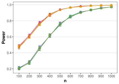
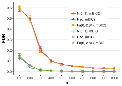
As you can see, both for the gaussian and subgaussian errors the power tends to one while FDR goes to zero, which implies the consistency. Because the penalty in mBIC2 is lower than in mBIC, the power for this criterion is higher, but FDR also. We observe similar behaviour for the Pareto distribution (which is not subgaussian), and this suggests that the theorems given in the previous section can be strengthened. For $n=200$ FDR is greater than 0.1 (although it has been previously stated that mBIC2 controls FDR), however, we must remember that the design matrix is โ€‹โ€‹non-orthogonal (the maximum absolute correlation between columns for the simulated data is 0.36).

4.1 Backcross design

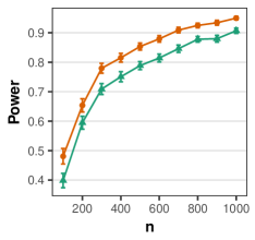
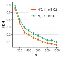
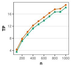
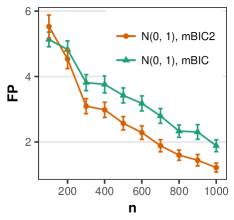
Recall that in the design matrix discussed above the elements were generated independently from the standard normal distribution. In actual genetic applications, there is often a situation in which columns of the design matrix are characterized by a high and slowly disappearing correlation, such as in the so called backcross design. In this case, predictors can take only two values and the correlation between columns $t$ and s๐‘ s is equal to expโก(โˆ’ฮฑโ€‹|tโˆ’s|)๐›ผ๐‘ก๐‘ \exp(-\alpha|t-s|), where $\alpha>0$. In order to illustrate that the criteria are also consistent in this situation, the individual columns (markers) were simulated according to the backcross, for $\alpha=0.04$. Other parameters were chosen as in previous simulations, only coefficients $\beta_{j}$ were increased to $8n^{-1/4}$, while genotypes of markers were coded as 0 and 1. The results are shown in the Figure 2. We see that the power goes to one, while the fraction of false discoveries goes to zero. It is interesting that this time mBIC2 has not only higher power but also lower FDR. This is not only due to the fact that mBIC2 finds more causal markers than mBIC, but also the number of false discoveries is smaller. This is illustrated by The Figure 3, on which the numbers of true and false discoveries were given instead of the power and FDR.

This phenomenon can be explained in such a way that when a model contains more causal markers, a precision of their location increases. Because the correlation between columns is high, the criteria find markers that are very close to causalโ€”but we count them as false discoveries. Models found by mBIC2 are larger, thanks to which a precision increases and this situation is rarer.

Figure 2: The power and FDR for data simulated according to the backcross design, after using mBIC and mBIC2. The vertical lines represent standard errors multiplied by the 0.975 quantile of the standard normal distribution.
Refer to caption
Refer to caption
Figure 3: The number of true and false discoveries for data simulated according to the backcross design, after using mBIC and mBIC2. The vertical lines represent standard errors multiplied by the 0.975 quantile of the standard normal distribution.
Refer to caption
Refer to caption

4.2 Package bigstep

We want to add few words about the package which was used in those simulations. It is worth noting that if we have 1000 observations and $10^{5}$ predictors, it is not easy to perform the stepwise procedure on such big data using home computers. What is more, it should be relatively quick because when we do simulations, we want to repeat this many times. That was a motivation to write the package bigstep. The most important feature of this package is that it does not load a whole design matrix to the memory, which is impossible when we have a lot of predictors, but instead it keeps this matrix on the hard drive and works only on a part of it (that is the package only loads as many columns as the computerโ€™s memory allows). When we check every predictor in that part, we go to the next one. It is possible because the stepwise is a sequential procedure, we do not need to have access to every predictor at the same time. Theoretically, the package should work with any number of variables. There is only one condition: models which are fitting in next steps cannot be too large, that is they cannot exceed the memory capacity. In practise, it is very hard to do that, especially when we are interested in sparse models.

5 Discussion

We gave conditions when mBIC and mBIC2 are consistent, both when the error term is gaussian or subgaussian. Theorems were supported by simulations and it should be emphasized that in all of them neither the size of the true model nor the number of all variables nor the size of $\beta_{j}$ were fixed (then this type of asymptotic behaviour of any reasonable criterion would be obvious). On the contrary: the size of the correct model and the number of all variables were increasing, while the magnitude of $\beta_{j}$ decreased. Furthermore, unlike EBIC and a lot of other criteria, mBIC and mBIC2 are precise, that is the penalty is accurate, does not depend on constants. It is important because in practice, asymptotic behaviour is not as important as FWER or FDR. If one is interested only on building models to perform good predictions, these constants can be selected using for example cross-validation, but it does not have to be a good practice when we are interested in the inference.

However, it is worth noting that in our simulations, when looking for the best model, we consider only a small part of them. As a result, some of the observed properties may not be a result of the characteristics of the criteria, but the method used to select a subset of the analyzed models. In a future work we want to show that the whole procedure, that is mBIC/mBIC2 and the stepwise, is consistent. We believe that this is true, based on a lot of simulations we have done and results of Su [11], who showed that if the design matrix is gaussian and a signal is sparse and strong enough, the forward selection gives us the appropriate ordering of variables.

References

  • [1] P. J. Bickel, Y. Ritov, A. B. Tsybakov. Simultaneous analysis of LASSO and Dantzig selector. Annals of Statistics, 39:1551โ€“1579, 2011.
  • [2] M. Bogdan, J.K. Ghosh, R.W. Doerge. Modifying the Schwarz Bayesian Information Criterion to locate multiple interacting quantitative trait loci. Genetics, 167:989โ€“999, 2004.
  • [3] E. Candรจs, T. Tao. The Dantzig selector: statistical estimation when p is much larger than n. Annals of Statistics, 35:2313โ€“2325, 2007.
  • [4] J. Chen, Z. Chen. Extended Bayesian Information criteria for model selection with large model spaces. Biometrika 95(3):759โ€“771, 2008.
  • [5] F. Frommlet, A. Chakrabarti, M. Murawska, M. Bogdan. Asymptotic Bayes optimality under sparsity for general distributions under the alternative, Technical report, arXiv:1005.4753v2, 2011.
  • [6] F. Frommlet, F. Ruhaltinger, P. Twarรณg, M. Bogdan. A model selection approach to genome wide association studies. Computational Statistics and Data Analysis, 56:1038โ€“1051, 2012.
  • [7] D. Hsu, S.M. Kakade, T. Zhang. A tail inequality for quadratic forms of subgaussian random vectors. Electronic Communications in Probability, 17:1โ€“6, 2012.
  • [8] S. Luo, Z. Chen. Extended BIC for linear regression models with diverging number of relevant features and high or ultra-high feature spaces. Journal of Statistical Planning and Inference, 143(3):494โ€“504, 2013.
  • [9] P. Pokarowski, J. Mielniczuk. Combined $l_{1}$ and Greedy $l_{0}$ Penalized Least Squares for Linear Model Selection. Journal of Machine Learning Research, 16:961โ€“992, 2015.
  • [10] G. Seber, A. Lee. Linear Regression Analysis. John Wiley and Sons, 2002.
  • [11] W. Su. When Does the First Spurious Variable Get Selected by Sequential Regression Procedures? arXiv:1708.03046, 2017 (to appear in Biometrika).
  • [12] P. Szulc. Weak conistency of modified versions of Bayesian Information Criterion in a sparse linear regression. Probability and Mathematical Statistics, 32:47โ€“55, 2012.
  • [13] S.S. Vempala, The Random Projection Method. DIMACS Series in Discrete Mathematics and Theoretical Computer Science, 65, 2005.
  • [14] M. ลปak-Szatkowska, M. Bogdan. Modified versions of Bayesian Information Criterion for sparse Generalized Linear Models. Computational Statistics and Data Analysis, 55:2908โ€“2924, 2011.