On the Nonlinear Evolution of Cosmic Web: Lagrangian Dynamics Revisited

Abstract

We investigate the nonlinear evolution of cosmic morphologies of the large-scale structure by examining the Lagrangian dynamics of various tensors of a cosmic fluid element, including the velocity gradient tensor, the Hessian matrix of the gravitational potential as well as the deformation tensor. Instead of the eigenvalue representation, the first two tensors, which associate with the ‘kinematic’ and ‘dynamical’ cosmic web classification algorithm respectively, are studied in a more convenient parameter space. These parameters are defined as the rotational invariant coefficients of the characteristic equation of the tensor. In the nonlinear local model (NLM) where the magnetic part of Weyl tensor vanishes, these invariants are fully capable of characterizing the dynamics. Unlike the Zel’dovich approximation (ZA), where various morphologies do not change before approaching a one-dimensional singularity, the sheets in NLM are unstable for both overdense and underdense perturbations. While it has long been known that the coupling between tidal tensor and velocity shear would cause a filamentary final configuration of a collapsing region, we show that the underdense perturbation are more subtle, as the balance between the shear rate (tidal force) and the divergence (density) could lead to different morphologies. Interestingly, this instability also sets the basis for understanding some distinctions of the cosmic web identified dynamically and kinematically. We show that the sheets with negative density perturbation in the potential based algorithm would turn to filaments faster than in the kinematic method, which could explain the distorted dynamical filamentary structure observed in the simulation.

1 Introduction

As a result of anisotropic gravitational instability, the matter distribution of the Universe at large scale exhibits an intrinsic pattern, known as the cosmic web (Bond et al., 1996). This particular structure, characterized by a network of filaments, sheets and empty voids, has repeatedly been revealed by various observations, including the large scale galaxies distribution from galaxies surveys (Gregory & Thompson, 1978; de Lapparent et al., 1986; Geller & Huchra, 1989; Shectman et al., 1996; Colless et al., 2003; Tegmark et al., 2004; Huchra et al., 2005) and the dark matter map inferred from weak lensing survey (Massey et al., 2007). In this regard, the presence of this structure in both numerical simulations and analytical models, e.g. the Zel’dovich approximation (ZA, Zel’dovich, 1970), highlights our achievement of understanding the process of structure formation.

Besides its significance in the theory of large-scale structure, the cosmic web also serves as an environment for small scale structures like halos and galaxies. Various observations suggest that many galaxy properties vary with this environment systematically (Dressler, 1980; Kauffmann et al., 2004; Blanton et al., 2005). Meanwhile, high-resolution numerical simulations also show clear correlations between halo properties, like concentration and spin, with the local environment (Lemson & Kauffmann, 1999; Sheth & Tormen, 2004; Avila-Reese et al., 2005; Wechsler et al., 2005; Bett et al., 2007; Macciò et al., 2007; Wetzel et al., 2007; Hahn et al., 2007a, b). Hence, it is essential to define properly and better understand this morphological environment and its time evolution.

Figure 1: Comparison between kinematic (middle panel) and dynamical (right panel) classification for one snapshot of N-body simulation with the density distribution shown in the first panel. Both velocity and gravitational potential fields have been smoothed by a Gaussian filter with characteristic scale $R=1{\rm Mpc}/h$ before applying the algorithm. The black, grey and silver regions illustrate knots, filaments and sheets respectively, while white shows the voids. Unlike some other works, we assume eigenvalue threshold $\lambda_{th}=0$ for both algorithms. Therefore, different morphologies identified here are not ‘optimized’ to match the visual impression. Furthermore, this snapshot is selected in particular to highlight the significant differences these two methods could produce. The simulation has a box size of $100~{}{\rm Mpc}/h$, with $256^{3}$ particles. Both density and velocity field was estimated with Delaunay tessellation (Bernardeau, & van de Weygaert, 1996; Schaap & van de Weygaert, 2000; Pelupessy et al., 2003).

Although this web structure originates from anisotropic initial random field (Doroshkevich, 1970) and is qualitatively well described by simple analytical model like ZA, its evolution, however, is highly nonlinear at later epoch. Consequently, many efforts have been concentrated on developing algorithms of morphology classification for numerically simulated data. At least two categories of such algorithms exist in literatures, one is geometrical method, which tries to establish a mathematical description based on the point samples of galaxies/halos or dark matter particles in simulations (Lemson & Kauffmann, 1999; Novikov et al., 2006; Aragón-Calvo et al., 2007; Sousbie et al., 2008). The other ‘dynamical/kinematic’ approach then considers the movement of a test particle in the inhomogeneous gravitational potential, which could either be described by the Hessian matrix of gravitational potential (Hahn et al., 2007a; Forero-Romero et al., 2009) or the velocity gradient tensor (Hoffman et al., 2012). Various morphologies can then be identified by the number of eigenvalues greater than some threshold value.

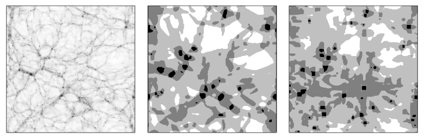
In Zel’dovich’s structure formation theory (Zel’dovich, 1970), these two tensors are simply proportional to each other, and therefore provide identical morphology classification. However, once the Universe enters into the nonlinear regime, differences start to emerge. With a similar level of smoothing and comparable eigenvalue thresholds, Hoffman et al. (2012) showed that the velocity based algorithm provides very different morphologies than the gravitational potential based technique and seems to resolve smaller structures (also in Figure. 1 for zero eigenvalue threshold). However, the reason of such dissimilarity is not clear, and theoretical investigation is highly demanded. Furthermore, instead of the null eigenvalue threshold first utilized by Hahn et al. (2007a), subsequent studies in general assume a nonzero threshold which is usually artificially tuned to provide the best visual impression. For gravitational potential based cosmic web, Forero-Romero et al. (2009) suggested that the threshold value of properly normalized tensor should be around unity based on the argument of spherical collapse. However, the justification requires more detailed study on the classification schemes and cosmic evolution of both tensors.

Compared with geometrical methods, where algorithmic procedures usually prevent them from further analytical understandings, one advantage of considering the dynamical variables is the potential to quantitatively investigate the cosmic web evolution, which however, has not been fully appreciated yet. One of the obstacles is the less-convenient eigenvalue representation of the algorithm. On the other hand, it is equivalent to study the eigenvalues and the rotational invariant coefficients of the characteristic equation of the tensor (Wang et. al., 2014). As shown by Wang et. al. (2014), the most important advantage of this parameter space is to avoid the complex domain after the tensor become non-symmetric. However, even for the purpose of this paper, where only the symmetric part is of interest, it will still be convenient to work in this invariant space. Especially, when the trace of the tensor does not change the sign, a two-dimensional subspace would suffice to present morphological evolution.

Figure 2: Illustration of cosmic web classification in the invariants space with various eigenvalue threshold $\lambda_{th}$. We only display two dimensional $s_{3}-s_{2}$ planes with fixed $s_{1}=-1$ (left) and $s_{1}=1$ (right). Regions with different transparencies highlight the consequences of varying eigenvalue threshold, assuming $s_{1}$ doesn’t change the sign. Since the boundary conditions depend on the value of $s_{1}$, we renormalize $s^{th}_{i}$ ($i=2$ or $3$) by $(s^{th}_{1})^{i}$ after the transformation equation (2.2) so that they remain the same. For more details of the invariants classification including rotational categories, please see Figure (1) in Wang et. al. (2014).

The main purpose of this paper is therefore to investigate theoretically in this invariant space, the nonlinear evolution of the velocity gradient tensor and the Hessian matrix of gravitational potential. Furthermore, to compare with geometrical algorithm, we will examine the evolution of the deformation tensor as well. To this end, we adopt the Lagrangian approach to track the dynamical evolution of relevant variables of a fluid element, including the density, the velocity gradient and the tidal tensor. However in Newtonian theory (NT), the evolution equation of the tidal tensor is missing. An alternative approach, as discussed by Bertschinger & Jain (1994) (hereafter denotes as ‘BJ94’), instead starts from the full general relativistic description, where the Lagrangian evolution equations and constraints of gravitational fields are well-known. Specifically, the evolution equation of the counterpart of the tidal tensor, i.e. the electric part of Weyl tensor, can be derived from the Bianchi identities. However, the treatment of the magnetic part of this tensor in NT is unclear and therefore triggered many discussions (Bertschinger & Hamilton, 1994; Ellis & Dunsby, 1997). Nevertheless, in the current paper, we will simply adopt the approach same as Bertschinger & Jain (1994), assuming the vanishing magnetic part of Weyl tensor, which produces a set of self-consistent (Lesame et al., 1995) closed ordinary differential equations.

In this model, the interaction of tensor perturbations between neighboring fluid elements is neglected, therefore also known as the ‘silent universe’ model. Since NT is intrinsically nonlocal as the potential is determined by the matter distribution everywhere via Poisson equation, a non-general relativistic theory with an extra time evolution equation of the tidal tensor should be regarded as some extension of NT, a closer approximation to the general relativity (Ellis & Dunsby, 1997). Practically, assuming a vanishing magnetic part of Weyl tensor would dramatically simplify the formalism (Matarrese et al., 1993; Matarrese, 1994; Bruni et al., 1995; Lesame et al., 1995). On the other hand, one obvious shortage of the Lagrangian approach is the existence of the singularity at the shell-crossing. It sets the validity range of the method much earlier than the formation of virialized objects. Fortunately, for our purpose, it is equally, if not more, important to study the underdense perturbations as the visual impression of the cosmic morphologies is highly weighted by the lower dense regions for their greater volume filling factors.

The paper is organized as follows. In section 2, we first briefly revisit two types of cosmic classification algorithms and then introduce the definition of rotational invariants as well as the geometrical quantities related to the deformation tensor. In section 3, we discuss Lagrangian dynamical evolution models. We first show the analytical results of invariants evolution in Zel’dovich approximation in section 3.1 and then review BJ94’s nonlinear local evolution model in section 3.2 before deriving the basic equation for obtaining the deformation tensor. We present our result in section 4 by first comparing the Zel’dovich approximation and the nonlinear local model. We then discuss the differences between velocity gradient tensor and Hessian matrix of gravitational potential in section 4.2. After discussing the eigenvalue threshold, we finally conclude in Section 5.

2 Cosmic Web Classification

We are interested in one particular category of cosmic web classification algorithm that considers the movement of a test particle in the anisotropic gravitational field. In an appropriate frame, this could either be described by the Hessian matrix of gravitational potential or the velocity gradient tensor. While the first characterizes the acceleration of the particle caused by the gravity, the latter describes the velocity changes. Both of them relate to the trajectories of the particle around given point by the time integral. Given the matrices, rotational invariants provide a more convenient parameter space for studying the sign of eigenvalues. For nonzero thresholds, however, the transformation of the invariants would be necessary, or equivalently the boundary condition among various morphologies need to be modified. To compare with other geometrical classification approaches, it is also valuable to examine the deformation tensor and derived scalars, e.g. the ellipticity and prolaticity. These scalars, usually well-defined in the linear region, require appropriate revision in the nonlinear regime.

2.1 Dynamical and Kinematic Approaches

As initiated by Hahn et al. (2007a) and followed by Forero-Romero et al. (2009), the dynamical approach considers the linearized equation of motion of a test particle near given position $\bar{\mathbf{x}}$

$$\frac{d^{2}x_{i}}{dt^{2}}=-\Phi_{i}^{~{}j}(\bar{\mathbf{x}})\left(\mathbf{x}_{j}-\bar{\mathbf{x}}_{j}\right),$$ (1)

where $\mathbf{x}$ is the comoving free-falling coordinate, $t$ is some time variable, $\Phi_{ij}=\partial_{i}\partial_{j}\Phi$ is the Hessian matrix of peculiar gravitational potential $\Phi$, and the zeroth-order term $\partial_{i}\Phi$ disappears in this frame. Therefore, the linear dynamics near location $\bar{\mathbf{x}}$ is fully characterized by tensor $\Phi_{ij}$, or as it’s real and symmetric, three eigenvalues of $\Phi_{ij}$. Then various morphologies could be classified by counting the number of eigenvalues greater than some threshold value. As motivated by this method, Hoffman et al. (2012) proposed a similar classification scheme based on the kinematic movement of the particle, also known as V-web, which is equivalent to considering the particle trajectory near $\bar{\mathbf{x}}$ as

$$\frac{dx_{i}}{d\tau}=A_{i}^{~{}j}(\bar{\mathbf{x}})\left(\mathbf{x}_{j}-\bar{\mathbf{x}}_{j}\right)$$ (2)

where $A_{ij}=\partial_{i}v_{j}$. Unlike the potential Hessian matrix $\Phi_{ij}$, in principle $A_{ij}$ could be rotational and therefore non-symmetric (Wang et. al., 2014). However, in this paper we will only concentrate on the symmetric part of $A_{ij}$, assuming $A_{ij}=A_{ji}$.

Both kinematic and dynamical approaches try to identify various cosmic structure by examining the tentative movement of the test particle. Intuitively, one would expect the deviation between these two approaches after entering into the nonlinear regime as the acceleration/deceleration of the particle towards a certain direction is not necessarily the same as the velocity. In Figure. (1), we compare these two algorithms in the numerical simulation. Before performing the classification, both velocity and potential fields have been smoothed by a Gaussian filter with the characteristic length $R=1{\rm Mpc}/h$. Unlike other works, here we assume the zero eigenvalue threshold for both tensors so that the cosmic web structure highlighted here would not be ‘optimized’ visually. From the figure, it is clear that these two methods produce very different classifications in details. Actually, we select this snapshot in particular to underline how significant these two approaches could differ. However, as will be shown in section 4, at least for filaments, the dissimilarity could be alleviated by restricting the trace of the tensor.

Figure 3: Comparison between Zel’dovich approximation (upper panels) and nonlinear local model (lower panels) in the velocity invariant space $s^{(v)}_{i}$. From left to right, we assume the linear density perturbation $\delta_{0}=-1,~{}-0.5,~{}1$ and $2$, where $\delta_{0}=\delta(a=1)$. To better present the result, we have normalized invariants $s^{(v)}_{i}$ such that ${\rm tr}[A_{ij}]=\pm 1$. For underdense perturbations all trajectories are plotted from the initial epoch $a_{0}=10^{-3}$ to the present $a=1$, while we stop at the first singularity for $\delta_{0}>0$.

2.2 Classification with Rotational Invariants

In practice, both approaches concern the number of eigenvalues of the tensor above a certain threshold $\lambda_{th}$. As proposed by Wang et. al. (2014), assuming $\lambda_{th}=0$, this problem could also be reformulated as considering the number of positive/negative solutions of characteristic equation $\det[\mathbf{T}-\lambda\mathbf{I}]=0$ of tensor $\mathbf{T}$, i.e.

$$\lambda^{3}+s_{1}\lambda^{2}+s_{2}\lambda+s_{3}=0,$$ (3)

where we assume $T_{ij}=A_{ij}$ for kinematic method and $-\Phi_{ij}$ for dynamical approach. The rotational invariant coefficients $s_{1},s_{2},s_{3}$ are defined as (Chong et al., 1990; Wang et. al., 2014)

$$s_{1} = -\rm tr[\mathbf{T}]=-T_{i}^{~{}i}=-\sum_{i}\lambda_{i},$$

$$s_{2} = \frac{1}{2}\left(s_{1}^{2}-\rm tr[\mathbf{T}^{2}]\right)=\frac{1}{2}(s_{1}^{2}-T_{ij}T^{ji})=\sum_{i\neq j}\lambda_{i}\lambda_{j}$$

$$s_{3} = -\det[\mathbf{T}]=\frac{1}{3}\left(-s_{1}^{3}+3s_{1}s_{2}-\rm tr[\mathbf{T}^{3}]\right)$$ (4)

$$= \frac{1}{3}\left(-s_{1}^{3}+3s_{1}s_{2}-T_{i}^{~{}j}T_{j}^{~{}k}T_{k}^{~{}i}\right)=-\prod_{i}\lambda_{i}.$$

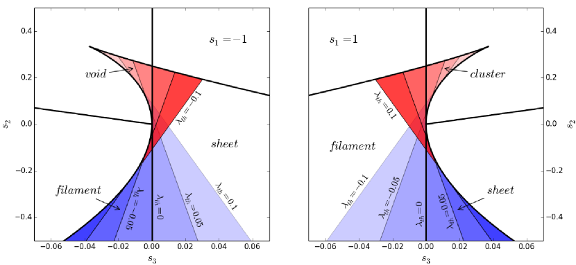
Here we have already neglected the anti-symmetric contribution of tensor $T_{ij}$, so that $T_{ij}=T_{ji}$. In the last equality of the definition, we have already expressed them in terms of real eigenvalues $\lambda_{i}$. In the following, we will denote $s^{v}$ as invariants constructed from $A_{ij}$ and $s^{\phi}$ as from $-\Phi_{ij}$. Then the conditions of having certain number of positive/negative eigenvalues, is mapped into various regions in the invariants space. In Figure. (2), we briefly illustrate these classifications in thick solid lines for both negative (left panel) and positive $s_{1}$ (right panel). In both cases, the triangular-like region with real eigenvalues is enclosed by the solution of equation (Chong et al., 1990; Wang et. al., 2014)

$$27s_{3}^{2}+(4s_{1}^{3}-18s_{1}s_{2})s_{3}+(4s_{2}^{3}-s_{1}^{2}s_{2}^{2})=0,$$ (5)

with the assumptions $s_{2}\leq s_{1}^{2}/3$. Within this region, different morphologies are basically determined by the sign of invariants. For $s_{1}<0$, region with $s_{2}>0$ and $s_{3}<0$ denotes the void, while condition $s_{2}<0,~{}s_{3}<0$ corresponds to the filament, and $s_{3}>0$ is cosmic sheet. Similarly for $s_{1}>0$, condition $s_{2}>0,~{}s_{3}>0$ defines the cluster, $s_{2}<0,~{}s_{3}>0$ corresponds to the sheet, and $s_{3}<0$ denotes the filament. Furthermore, it is worth noticing that the classification would remain the same if the invariants are rescaled as

$$\tilde{s}_{i}=s_{i}/(c)^{i},\qquad where~{}c>0$$ (6)

by any positive constant $c$, since the normalization of $T_{ij}$ with $c$ would not change the sign of its eigenvalues. Please see Wang et. al. (2014) for more details of the invariants-based cosmic web classification.

For a nonzero eigenvalue threshold $\lambda_{th}$, however, one could define the eigenvalue $\lambda^{\prime}=\lambda-\lambda_{th}$, and rewrite the characteristic equation (3) as function of $\lambda^{\prime}$,

$$(\lambda^{\prime}+\lambda_{th})^{3}+s_{1}(\lambda^{\prime}+\lambda_{th})^{2}+s_{2}(\lambda^{\prime}+\lambda_{th})+s_{3}=0,$$ (7)

and then discuss the sign of variable $\lambda^{\prime}$. Expanding equation (7), it is equivalent to define a new set of invariants $s^{th}$ as (Wang et. al., 2014),

$$s^{th}_{1} = s_{1}+3\lambda_{th}$$

$$s^{th}_{2} = s_{2}+2\lambda_{th}s_{1}+3\lambda_{th}^{2}$$

$$s^{th}_{3} = s_{3}+\lambda_{th}s_{2}+\lambda_{th}^{2}s_{1}+\lambda_{th}^{3}.$$ (8)

Then all classification conditions of the invariants remain the same. Alternatively, with the help of equation (2.2), one could also express all conditions back into the original invariants space. Since any linear combination of real eigenvalues with a real threshold $\lambda_{th}$ remains real, the boundary condition separating real and complex solutions does not need to vary in the transformed three-dimensional invariant space $s^{th}_{i},~{}i=\{1,2,3\}$. However, for illustrative purpose, we are also interested in the two-dimensional $s^{th}_{3}-s^{th}_{2}$ subspace as displayed in Figure (2), where the real-image separation surface would project onto $s^{th}_{1}=const$ plane differently. But if the sign of $s^{th}_{1}$ remains the same, one could simply rescale the invariants so that $s^{th}_{1}$ is unchanged (e.g. $s^{th}_{1}=\pm 1$), and the same for the boundary in the $s^{th}_{3}-s^{th}_{2}$ plane. Then various morphologies within this region would be classified based on the sign of $s_{3}^{th}$ and its intersection with one of the solution in equation (5).

In Figure (2), we also illustrate the effect of varying the threshold $\lambda_{th}$ in the same two-dimensional invariants subspace, assuming $s^{th}_{1}$ does not change the sign. The thin solid lines correspond to the transformed equation $s^{th}_{3}=0$, and various morphological regions with different $\lambda_{th}$ are then enclosed by these lines and thick solid boundaries. For example, void or cluster are still those triangular regions, but with the original vertical condition $s_{3}=0$ changing accordingly. In each panel, we also set the transparency level to each threshold value for different colored (morphological) regions consistently. As could be seen, a negative $\lambda_{th}$ will enlarge the region classified as void, and shrink the region of cluster and oppositely for positive $\lambda_{th}$. For sheet and filament, however, they will be affected a little more complicated. As sheets with positive $s_{1}$ become more abundant with negative $\lambda_{th}$, regions tagged as sheet with negative $s_{1}$ at $\lambda_{th}=0$ might become voids, and some filamentary regions will then be identified as sheet. Meanwhile, filamentary regions with $s_{1}<0$ will be reduced, and some filaments with $s_{1}>0$ at $\lambda_{th}=0$ will be classified as sheets. On the other hand, a few cluster regions will turn to this type; and positive threshold would behave oppositely.

2.3 Deformation Tensor

Besides the classification based on $\Phi_{ij}$ and $A_{ij}$, it will also be helpful to examine the deformation tensor as well, as it characterizes the geometric deformation of a fluid element during the evolution. The tensor is defined as

$$\Psi_{ij}=\frac{\partial\Psi_{i}}{\partial q_{j}}=J_{ij}-I_{ij}.$$ (9)

Here the displacement vector $\Psi_{i}=x_{i}-q_{j}$, where $x_{i}$ is the Eulerian position and $q_{i}$ is initial Lagrangian coordinate. $J_{ij}=\partial x_{i}/\partial q_{j}$ is the Jacobian matrix between $q_{i}$ and $x_{i}$, and $I_{ij}$ is the identity matrix. Unlike classification algorithms introduced previously, tensor $\Psi_{ij}$ characterizes the changes in shape and size of the fluid element. Hence, it would be convenient to define the geometric quantities like the ellipticity and prolaticity from $\Psi_{ij}$. For Zel’dovich approximation, where all eigenvalues of $\Psi_{ij}$ grow linearly, they are defined as (Bond et al., 1996)

$$e^{\lambda}=\frac{\lambda^{\psi}_{3}-\lambda^{\psi}_{1}}{|\lambda^{\psi}_{1}+\lambda^{\psi}_{2}+\lambda^{\psi}_{3}|},\qquad p^{\lambda}=\frac{\lambda^{\psi}_{1}+\lambda^{\psi}_{3}-2\lambda^{\psi}_{2}}{|\lambda^{\psi}_{1}+\lambda^{\psi}_{2}+\lambda^{\psi}_{3}|},$$ (10)

assuming $\lambda^{\psi}_{3}\geq\lambda^{\psi}_{2}\geq\lambda^{\psi}_{1}$, where $\lambda^{\psi}_{i}$ are eigenvalues of deformation tensor $\Psi_{ij}$. However, for nonlinear evolution, it is possible that the denominator $\sum_{i}\lambda^{\psi}_{i}$ changes the sign during the cosmic evolution . Therefore, $e^{\lambda}$ and $p^{\lambda}$ could be singular even before the shell-crossing. Therefore, in this paper, we recover the full definition of the nonlinear ellipticity and prolaticity by substituting the denominator with its nonlinear counterpart $|J-1|=|\delta|$

$$e^{J}=\frac{\lambda^{\psi}_{3}-\lambda^{\psi}_{1}}{|J-1|},\qquad p^{J}=\frac{\lambda^{\psi}_{1}+\lambda^{\psi}_{3}-2\lambda^{\psi}_{2}}{|J-1|},$$ (11)

where $J$ is the determinant of the Jacobian $J_{ij}$. For $|\delta|\ll 1$, these two equations are equivalent, and $|J-1|=\prod_{i}\lambda^{\psi}_{i}$ would keep the sign before the shell-crossing. One notices that the boundary condition $e^{J}\geq 0$ and $-e^{J}\leq p^{J}\leq e^{J}$ are still valid. In the following, we will omit superscripts and simply denote $e$ and $p$ as defined in equation (11).

Figure 4: Detailed morphology comparison between kinematic web (upper panels) and dynamical web (lower panels), assuming threshold $\lambda_{th}=0$. From left to right, different panels highlight morphologies types of (a) filaments with positive $s^{v/\phi}_{1}$, (b) filaments with negative $s^{v/\phi}_{1}$, (c) sheets with negative $s^{v/\phi}_{1}$ and (d) sheets with positive $s^{v/\phi}_{1}$. Although the filamentary structure presented in Figure. (1) are very different, regions shown in the first column are quite similar between these two algorithms. The distortion of the dynamical filaments is due to the contribution from the second column, i.e. filaments with negative $s^{(v/\phi)}_{1}$.

3 Lagrangian Dynamics

In this section, we will briefly review the Lagrangian evolution of a fluid element in Newtonian cosmology, especially concentrate on the evolution of the velocity gradient tensor $A_{ij}$ and the Hessian matrix of gravitational potential $\Phi_{ij}$. Before the shell-crossing, the dynamical equations could be expressed as continuity equation, Euler equation as well as Poisson equation (Peebles, 1980; Bernardeau et al., 2002),

$$\frac{\partial\delta}{\partial\tau}+\nabla\cdot[(1+\delta)\mathbf{v}]=0,\qquad\qquad\qquad\qquad$$

$$\frac{\partial\mathbf{u}}{\partial\tau}+\mathcal{H}(\tau)\mathbf{u}(\mathbf{x},\tau)+\mathbf{u}(\mathbf{x},\tau)\cdot\nabla\mathbf{u}(\mathbf{x},\tau)=-\nabla\Phi(\mathbf{x},\tau)\qquad$$

$$\nabla^{2}\Phi(\mathbf{x},\tau)=4\pi G\bar{\rho}~{}\delta(\mathbf{x},\tau).\qquad\qquad\qquad\qquad$$ (12)

As we are interested in the Lagrangian evolution in this paper, the continuity equation could be further expressed as

$$\frac{d\delta}{d\tau}+(1+\delta)\theta=0,$$ (13)

where $d/d\tau$ is Lagrangian total derivative, and $\theta=\nabla\cdot\mathbf{u}$ is the velocity divergence. It is then necessary to consider the Lagrangian equation of the velocity gradient tensor $A_{ij}$, which could simply be obtained by taking the gradient of the second equation in equation (3)

$$\frac{dA_{ij}}{d\tau}+\mathcal{H}(\tau)A_{ij}+A_{i}^{~{}k}A_{kj}=-\Phi_{ij}$$ (14)

Following the standard treatment, the source term $\Phi_{ij}$ is decomposed as the trace $\nabla^{2}\Phi$ and the traceless part $\varepsilon_{ij}=\Phi_{ij}-I_{ij}\nabla^{2}\Phi/3$. While the trace $\nabla^{2}\Phi$ simply relates to the density via Poisson equation, however, no time evolution equation exists for the $\varepsilon_{ij}$ in the Newtonian cosmology. However, it is possible to write down the evolution and constraint equations for all gravitational fields in general relativity, including the tidal tensor or the electric part of Weyl tensor $\varepsilon_{ij}$ (Ellis, 1971; Matarrese et al., 1993; Bertschinger & Jain, 1994),

$$\frac{d}{d\tau}\varepsilon_{ij}+\mathcal{H}(\tau)\varepsilon_{ij}+\theta\varepsilon_{ij}+I_{ij}\sigma^{kl}\varepsilon_{kl}-3\sigma^{k}_{~{}(i}\varepsilon_{j)k}\qquad\qquad$$

$$+\epsilon^{kl}_{~{}~{}(i}\varepsilon_{j)k}\omega_{l}-\nabla_{k}\epsilon^{kl}_{~{}~{}(i}\mu_{{j)l}}=-4\pi G\rho a^{2}\sigma_{ij},\qquad$$ (15)

where $\sigma_{ij}=A_{ij}-\theta I_{ij}/3$ is the traceless velocity shear tensor, $\omega_{ij}$ is the antisymmetric vorticity tensor, $\mu_{ij}$ is the magnetic part of Weyl tensor. Parenthesized subscripts denote the symmetrization, and $\epsilon_{ijk}$ is the total antisymmetric Levi-Civita tensor. Without the terms involving $\mu_{ij}$, the equation is pure local and therefore closed together with equation (13) and (14). On the other hand, with the non-vanishing $\mu_{ij}$ term, the dynamics of the tidal tensor and velocity gradient become much more complicated (Ellis, 1971; Bertschinger & Jain, 1994). Therefore in the following, we will simply assume $\mu_{ij}=0$.

Finally, given the evolution of $A_{ij}$ in Eq. (14), the evolution equation of invariants $s^{v}_{i}$ of velocity could be derived straightforwardly (Wang et. al., 2014)

$$\frac{d}{d\tau}s^{v}_{1}+\mathcal{H}(\tau)s^{v}_{1}-(s^{v}_{1})^{2}+2s^{v}_{2}=\Phi_{i}^{~{}i}$$

$$\frac{d}{d\tau}s^{v}_{2}+2\mathcal{H}(\tau)s^{v}_{2}-s^{v}_{1}s^{v}_{2}+3s^{v}_{3}=s^{v}_{1}\Phi_{i}^{~{}i}+\Phi_{ij}A^{ji}$$

$$\frac{d}{d\tau}s^{v}_{3}+3\mathcal{H}(\tau)s^{v}_{3}-s^{v}_{1}s^{v}_{3}=s^{v}_{2}\Phi_{i}^{~{}i}+s^{v}_{1}\Phi_{ij}A^{ji}+\Phi_{i}^{~{}j}A_{j}^{~{}k}A_{k}^{~{}i}$$

3.1 Zel’dovich Approximation

In Lagrangian dynamics, the mass element moves in the gravitational field along the trajectory

$$\mathbf{x}(\mathbf{q},\tau)=\mathbf{q}+\mathbf{\Psi}(\mathbf{q},\tau),$$ (17)

from the initial Lagrangian position $\mathbf{q}$ to Eulerian coordinate $\mathbf{x}$, where $\mathbf{\Psi}$ is the displacement. To the first order, i.e. the Zel’dovich approximation, the displacement $\mathbf{\Psi}(\mathbf{q},\tau)$ is simply given by (Zel’dovich, 1970)

$$\nabla_{q}\cdot\Psi(\mathbf{q},\tau)=-D(\tau)\delta(\mathbf{q}),$$ (18)

where $D(\tau)$ the linear growth factor of density perturbation, and $\nabla_{q}$ denotes the spatial gradient with respect to Lagrangian coordinate. In Eulerian space, this is equivalent to replacing the Poisson equation with (Munshi, 1994; Hui & Bertschinger, 1996; Bernardeau et al., 2002)

$$u_{i}(\mathbf{x},\tau) = -\frac{2f(\tau)}{3\Omega_{m}(\tau)\mathcal{H}(\tau)}\nabla_{i}\Phi(\mathbf{x},\tau),$$ (19)

which then closes the system together with Euler equation (3). Here, $\Omega_{m}(\tau)$ is the matter density fraction at epoch $\tau$, and $f=d\ln D/d\ln a$ is the linear growth rate. Therefore simply by taking gradient of equation (19), one finds $A_{ij}$ and $\Phi_{ij}$ are proportional to each other

$$A_{ij} = -\frac{2f(\tau)}{3\Omega_{m}(\tau)\mathcal{H}(\tau)}\Phi_{ij},$$ (20)

Meanwhile since $A_{ij}$ relates to deformation tensor by

$$A_{ij}=\mathcal{H}f[\Psi_{i}^{~{}k}(I_{kj}+\Psi_{kj})^{-1}],$$ (21)

one could also derive the relation between $\Psi_{ij}$ and $\Phi_{ij}$

$$\Phi_{ij}=-\frac{3\Omega_{m}}{2}\mathcal{H}^{2}\Psi_{ij}$$ (22)

given $\Psi_{ij}$ is small.

Because of equation (20), we will only concentrate on the evolution of the velocity invariants $s^{v}$ in the rest of the section. As shown in Wang et. al. (2014), the dynamics of $A_{ij}$ can also be derived starting from the simplified Euler equation

$$\bar{\mathbf{u}}^{\prime}=\frac{d\bar{\mathbf{u}}}{dD}=\left(\frac{\partial}{\partial D}+\bar{\mathbf{u}}\cdot\nabla\right)\bar{\mathbf{u}}=0,$$ (23)

where we have defined the rescaled velocity $\bar{\mathbf{u}}=\mathbf{u}/D^{(v)}$ where $D^{(v)}(\tau)=dD/d\tau=\mathcal{H}fD$, and change the time variable $\tau$ into the linear growth rate $D$. For the velocity gradient tensor, we similarly define the rescaled quantity $\bar{A}_{ij}=A_{ij}/D^{(v)}$, and obtain

$$\frac{d\bar{A}_{ij}}{dD}+\bar{A}_{i}^{~{}k}\bar{A}_{kj}=0.$$ (24)

Therefore, the rescaled velocity invariants $\bar{s}^{v}_{1},\bar{s}^{v}_{2},\bar{s}^{v}_{3}$ is then defined as

$$\bar{s}^{v}_{i}(\tau)=\frac{s^{v}_{i}(\tau)}{[D^{(v)}]^{i}},\qquad i\in\{1,2,3\}.\quad$$ (25)

One can then derive a set of ordinary differential equations of reduced invariants:

$$(\bar{s}^{v}_{1})^{\prime}-(\bar{s}^{v}_{1})^{2}+2\bar{s}^{v}_{2} = 0,$$

$$(\bar{s}^{v}_{2})^{\prime}-\bar{s}^{v}_{1}\bar{s}^{v}_{2}+3\bar{s}^{v}_{3} = 0,$$

$$(\bar{s}^{v}_{3})^{\prime}-\bar{s}^{v}_{1}\bar{s}^{v}_{3} = 0.$$ (26)

As shown by Wilczek (2010), the analytic solution of Eq. (3.1) could be obtained by taking the third order derivative of $(1/\bar{s}^{v}_{3})$. Abbreviating time variable as $D-D_{i}=d$, the solution is expressed as

$$\bar{s}^{v}_{1}(d) = \frac{3\bar{s}^{v}_{3}(d_{0})d^{2}-2\bar{s}^{v}_{2}(d_{0})d+\bar{s}^{v}_{1}(d_{0})}{-\bar{s}^{v}_{3}(d_{0})d^{3}+\bar{s}^{v}_{2}(d_{0})d^{2}-\bar{s}^{v}_{1}(d_{0})d+1}$$

$$\bar{s}^{v}_{2}(d) = \frac{-3\bar{s}^{v}_{3}(d_{0})d+\bar{s}^{v}_{2}(d_{0})}{-\bar{s}^{v}_{3}(d_{0})d^{3}+\bar{s}^{v}_{2}(d_{0})d^{2}-\bar{s}^{v}_{1}(d_{0})d+1}$$

$$\bar{s}^{v}_{3}(d) = \frac{\bar{s}^{v}_{3}(d_{0})}{-\bar{s}^{v}_{3}(d_{0})d^{3}+\bar{s}^{v}_{2}(d_{0})d^{2}-\bar{s}^{v}_{1}(d_{0})d+1}.$$ (27)

Therefore in this model, the singularity occurs when the common denominator $-\bar{s}^{v}_{3}(d_{0})d^{3}+\bar{s}^{v}_{2}(d_{0})d^{2}-\bar{s}^{v}_{1}(d_{0})d+1$ becomes zero. one also notices that, after rescaling the invariants $\bar{s}^{v}_{2}$ and $\bar{s}^{v}_{3}$ by $|\bar{s}^{v}_{1}|^{i}$, where $i=(2,3)$, these two invariants would approach zero around the singularity. Finally, since $s^{v}_{3}$ never change the sign before singularity, cosmic web morphology would remain the same under the assumption that $\lambda_{th}=0$.

3.2 Nonlinear Local Evolution Model

3.2.1 Dynamics

Assuming irrotational dust model and vanishing magnetic Weyl tensor, equation (3) is simplified as

$$\frac{d}{d\tau}\varepsilon_{ij}+\mathcal{H}(\tau)\varepsilon_{ij}+\theta\varepsilon_{ij}+I_{ij}\sigma^{kl}\varepsilon_{kl}\qquad\qquad\qquad$$

$$\qquad\qquad-3\sigma^{k}_{~{}(i}\varepsilon_{j)k}=-4\pi G\rho a^{2}\sigma_{ij}.$$ (28)

Following Bertschinger & Jain (1994), one could conveniently parametrize tensor $A_{ij}$ and $\Phi_{ij}$ as

$$A_{ij} = \frac{1}{3}\theta I_{ij}+\frac{2}{3}\sigma Q_{ij}(\alpha)=\frac{1}{3}[\theta I_{ij}+2\sigma Q_{ij}(\alpha)]$$

$$\Phi_{ij} = \frac{4\pi}{3}G\bar{\rho}a^{2}[\delta I_{ij}+2\varepsilon(1+\delta)Q_{ij}(\beta)]$$ (29)

where $\sigma\leq 0$, $\varepsilon\geq 0$ are shear and tidal scalar respectively. $\alpha$ and $\beta$ are shear and tides angle, which give the ratios of eigenvalues of the shear and tidal tensors. The one-parameter traceless matrix is defined as

$$Q_{ij}(\alpha)={\rm diag}\left[\cos\left(\frac{\alpha+2\pi}{3}\right),\cos\left(\frac{\alpha-2\pi}{3}\right),\cos(\frac{\alpha}{3})\right].$$ (30)

This definition is uniquely determined by requirements of vanishing trace, $Q_{ij}Q^{ji}=3/2$ and $\det[Q_{ij}(\alpha)]=\cos\alpha$. Therefore, all possible eigenvalues of traceless matrix could be characterized by $qQ_{ij}(\alpha)$ with $q\in[0,\infty]$ and $\alpha\in[0,\pi]$. As shown in Bertschinger & Jain (1994), the matrix also have the following property

$$dQ_{ij}(\alpha) = \frac{1}{3}Q_{ij}\left(\alpha+\frac{3\pi}{2}\right)d\alpha,$$

$$2Q_{i}^{~{}k}(\alpha)Q_{kj}(\beta) = \cos\left(\frac{\alpha-\beta}{3}\right)I_{ij}+Q_{ij}(-\alpha-\beta).$$ (31)

With this parameterization, the Lagrangian equations of motion could be simplify as

$$\frac{d\sigma}{d\tau}+\mathcal{H}\sigma+\frac{1}{3}\sigma(2\theta+\sigma\cos\alpha)=\qquad\qquad\qquad\qquad\quad$$

$$-4\pi G\bar{\rho}a^{2}\varepsilon(1+\delta)\cos\left(\frac{\alpha-\beta}{3}\right)\quad$$

$$\frac{d\alpha}{d\tau}-\sigma\sin\alpha=12\pi G\bar{\rho}a^{2}\frac{\varepsilon(1+\delta)}{\sigma}\sin\left(\frac{\alpha-\beta}{3}\right)\qquad~{}$$

$$\frac{d\varepsilon}{d\tau}-\sigma\varepsilon\cos\left(\frac{\alpha+2\beta}{3}\right)=-\sigma\cos\left(\frac{\alpha-\beta}{3}\right)\qquad\qquad$$

$$\frac{d\beta}{d\tau}+3\sigma\sin\left(\frac{\alpha+2\beta}{3}\right)=-\frac{3\sigma}{\varepsilon}\sin\left(\frac{\alpha-\beta}{3}\right).\qquad\quad$$ (32)

Together with the Raychaudhuri equation for $\theta$

$$\frac{d\theta}{d\tau}+\mathcal{H}(\tau)\theta+\frac{1}{3}\theta^{2}+\frac{2}{3}\sigma^{2}=-4\pi G\bar{\rho}a^{2}\delta$$ (33)

and the continuity equation (13), the system is closed. Once the solution of physical variables is obtained, one could then derive the evolution of velocity invariants $s^{v}_{i}$

$$s^{v}_{1} = -\theta$$

$$s^{v}_{2} = \frac{1}{3}(\theta^{2}-\sigma^{2})$$

$$s^{v}_{3} = \frac{1}{27}(-\theta^{3}+3\theta\sigma^{2}-2\sigma^{3}\cos\alpha)$$ (34)

as well as the potential invariants $s^{\phi}_{i}$ from $\Phi_{ij}$

$$s^{\phi}_{1} = \delta$$

$$s^{\phi}_{2} = \frac{1}{3}\left[\delta^{2}-\varepsilon^{2}(1+\delta)^{2}\right]$$

$$s^{\phi}_{3} = \frac{1}{27}\left[\delta^{3}-3\delta\varepsilon^{2}(1+\delta)^{2}+2\varepsilon^{3}(1+\delta)^{3}\cos\beta\right]$$ (35)

Simply by counting the number of dynamical variables, one notices that our invariants $\{s^{v}_{i},s^{\phi}_{i}\},~{}i=(1,2,3)$ of both $A_{ij}$ and $\Phi_{ij}$ fully characterize this nonlinear dynamical model described by physical variables $\{\delta,\theta,\sigma,\varepsilon,\alpha,\beta\}$.

Figure 5: Comparison between kinematic (upper panels, defined by tensor $A_{ij}$) and dynamical (lower panels, defined by $\Phi_{ij}$) classification in the invariant space for nonlinear local model. From left to right, we assume $\delta_{0}=-1,~{}-0.5,~{}1$ and $2$. The same as Figure (3), we have normalized invariants $s^{(v/\phi)}_{i}$ such that ${\rm tr}[A_{ij}]={\rm tr}[-\Phi_{ij}]=\pm 1$. For underdense perturbation $\delta_{0}<0$, both tensors exhibit sheet instability, as trajectories flow towards voids or filaments, depending the initial conditions. However, trajectories in $s^{(\phi)}$ space tends to squeeze towards the boundary separating real and complex solutions. For the overdense perturbation, the singularity of $s^{(v)}$ occurs at $s^{(v)}_{2}=0$, while both $s^{(\phi)}_{2}$ and $s^{(\phi)}_{3}$ approach infinity.

3.2.2 Initial Condition

To specify the initial condition, we first notice that at the linear order

$$\theta=-\dot{\delta},\qquad\alpha=\beta,\qquad\sigma_{ij}\propto\epsilon_{ij}.$$ (36)

Therefore, among initial values of all six dimensional variable space $\{\delta_{0},\theta_{0},\sigma_{0},\epsilon_{0},\alpha_{0},\beta_{0}\}$, only three of them need to be identified initially, either $\{\delta_{0},\epsilon_{0},\beta_{0}\}$ or $\{\theta_{0},\sigma_{0},\alpha_{0}\}$. Particularly, for density and velocity divergence, one has

$$\theta_{0}=-\frac{d\ln D}{d\tau}(\tau_{0})~{}\delta(\tau_{0})=-\mathcal{H}_{0}f_{0}\delta_{0}$$ (37)

For tidal tensor, since $\alpha_{0}=\beta_{0}$ initially, to the linear order, one obtains the second-order differential equation of $\varepsilon$ the same as the density perturbation $\delta$

$$\ddot{\epsilon}(\tau)+\mathcal{H}(\tau)\dot{\epsilon}(\tau) = \frac{3}{2}\mathcal{H}(\tau)\Omega_{m}(\tau)\epsilon(\tau)$$

$$\sigma = -\dot{\epsilon}(\tau).$$ (38)

Therefore, $\varepsilon\propto D(\tau)$ at the first order, where $D(\tau)$ is the linear density growth rate. And similarly $\sigma_{0}$ relates to $\epsilon_{0}$ via $\sigma_{0}=-\mathcal{H}_{0}f_{0}\epsilon_{0}$. Moreover, it is also equivalent to specify e.g. the velocity invariants $\{s^{v}_{1},s^{v}_{2},s^{v}_{3}\}$ via

$$\theta(\tau_{0}) = -s^{v}_{1}~{}(\tau_{0})$$

$$\sigma(\tau_{0}) = -\sqrt{(s^{v}_{1})^{2}-3s^{v}_{2}}~{}(\tau_{0})$$

$$\cos\alpha(\tau_{0}) = \frac{2(s^{v}_{1})^{3}-9s^{v}_{1}s^{v}_{2}+27s^{v}_{3}}{2[(s^{v}_{1})^{2}-3s^{v}_{2}]^{3/2}}~{}(\tau_{0}).$$ (39)

3.3 Nonlinear Deformation Tensor

After solving the dynamical system, one is also able to derive the evolution of deformation tensor. Before multi-streaming, the displacement of a particle relates to the velocity simply by equation $x_{i}(\mathbf{q},\tau)=q_{i}+\int_{\tau_{0}}^{\tau}v_{i}(\tau^{\prime})d\tau^{\prime}$. By taking both the spatial gradient with respect to $q_{i}$ and the time derivative to this equation, one derives the differential equation of the Jacobian matrix $J_{ij}$

$$\frac{dJ_{ij}}{d\tau}=A_{i}^{~{}k}J_{kj}.$$ (40)

Assuming the tensor $J_{ij}$ and $A_{ij}$ could be simultaneously diagonalized, and denoting their eigenvalues as $\eta_{i}$ and $\lambda_{i}$ respectively, the solution of above equation could simply be expressed as,

$$\eta_{i}(\tau) = \eta_{i}(\tau_{0})\exp\left[\int_{\tau_{0}}^{\tau}\lambda_{i}(\tau^{\prime})d\tau^{\prime}\right]$$ (41)

$$= \eta_{i}(a_{0})\exp\left[\int_{a_{0}}^{a}\frac{\lambda_{i}(a^{\prime})}{a^{\prime}\mathcal{H}(a^{\prime})}da^{\prime}\right]$$

where the initial value $\eta_{i}(a_{0})$ relates to that of $\lambda_{i}(a_{0})$ as

$$\eta_{i}(a_{0})=\frac{1}{1-\tilde{\lambda}_{i}(a_{0})},\quad where~{}\lambda_{i}(a_{0})=\tilde{\lambda}_{i}(a_{0})\frac{d\ln D}{d\tau}(a_{0})$$ (42)

and $d\ln D/d\tau=\mathcal{H}f$. One could easily check that above equation holds for Zel’dovich approximation.

Figure 6: The evolution of ellipticity $e$ and prolaticity $p$ colored by kinematic (upper panels) and dynamical (lower panels) classification algorithms, assuming threshold eigenvalue $\lambda_{th}=0$. All trajectories are calculated via equation (40) with $A_{ij}$ supplemented by the nonlinear local model. Morphological evolutions are displayed by segmented color arrows, with the discontinuity point indicating the epoch of the transition.

4 The Evolution of Cosmic Web

Given the dynamical equations presented in the last section, one could simply integrate the set of ordinary differential equations with appropriate initial condition. In this section, we will present our results for both velocity and potential invariants in Zel’dovich approximation as well as the nonlinear local model. After comparing these two models in section 4.1, we will mainly concentrate on the latter and discuss the differences between the dynamical and kinematic morphology classifications in section 4.2. In section 4.3, we will then briefly comment on the practical freedom of eigenvalue threshold $\lambda_{th}$ and the ambiguity of the cosmic web definition.

4.1 From Zel’dovich Approximation to the Nonlinear Evolution of Cosmic Web

The pioneering work of the cosmic web evolution by Zel’dovich (1970) starts with the density perturbation as a function of linear growing eigenvalues of the deformation tensor $1+\delta=1/\prod_{i}[1+D(\tau)\lambda^{\psi}_{i}(\tau_{0})]$, with $\lambda^{\psi}_{i}$ being the eigenvalue of tensor $\Psi_{ij}$. Despite its simplicity, it suggests that the gravitational collapse would generally approach a one-dimensional ‘plane-parallel’ singular solution first as the probability measure of having two or more same eigenvalues is zero. Kinematically, however, since the deformation tensor $\Psi_{ij}$ grows linearly, the speed of the collapse is the same for all eigenvalues. It means that the morphological type inferred from $A_{ij}$ and $\Phi_{ij}$ would always be the same before reaching the singularity. This statement is valid for both overdense and underdense regions, as already seen from the analytical solution (3.1) of $s_{i}$ in ZA and subsequent discussions thereafter.

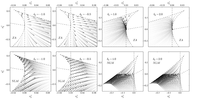
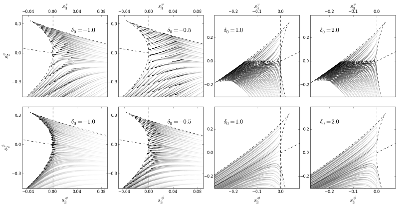
In the first row of Figure (3), we display the evolution trajectories in the invariant space for this model. For better presenting the result, all invariants are normalized according to equation (6) with the constant $c=|s_{1}|$ so that $\tilde{s}_{1}$ would only take values $1$ or $-1$. From left to right, different panels assume various initial conditions characterized by the linear density perturbation $\delta_{0}$ at $a=1$. For $\delta_{0}<0$, we plot all trajectories from initial epoch $a_{0}=10^{-3}$ to the present $a=1$; however, for $\delta_{0}>0$, they will end until the first singularity. In the first two panels, all trajectories simply diverge from the origin in the $s_{2}-s_{3}$ plane without changing categories. On the other hand, the overdense trajectories approach the first shell-crossing as $s^{v}_{2}/(s^{v}_{1})^{2}\to 0$ and $s^{v}_{3}/(s^{v}_{1})^{3}\to 0$. It corresponds to a characteristic equation $\lambda^{2}(\lambda+1)=0$, indicating a one-dimensional collapse with no motion in the other two dimensions. Since eigenvalues of $A_{ij}$ are proportional to $D(\tau)\xi_{i}(\tau_{0})/[1+D(\tau)\xi_{i}(\tau_{0})],~{}i\in\{1,2,3\}$, this occurs when the smallest eigenvalue goes toward $-\infty$ while the other two are still finite.

On the other hand, as already noticed by Croudace et al. (1994) and Bertschinger & Jain (1994), unlike in ZA, the gravitational collapse in the nonlinear local model would generally approach filamentary solution, and the sheet structure is usually unstable. Although Croudace et al. (1994) attributed it to the neglect of the magnetic part of Weyl tensor $\mu_{ij}$, Bertschinger & Jain (1994) suggested that the nonlinear coupling between velocity shear $\sigma_{ij}$ and tidal tensor $\varepsilon_{ij}$ in equation (3.2.1), i.e. the term $3\sigma^{k}_{~{}(i}\varepsilon_{j)k}-I_{ij}\sigma^{kl}\varepsilon_{kl}$, is responsible for this instability. Following their arguments, this term with sheet configuration $\alpha\approx\beta\approx 0$, has the signature opposite to the sign of $\varepsilon_{ij}$ and therefore slows down the growth of tides. Whereas filamentary configuration with $\alpha\approx\beta\approx\pi$, on the contrary, would grow due to this term. This could also be seen from the third equation of (3.2.1), given that $\cos((\alpha+2\beta)/3)$ approaches unity during the collapse.

In the invariants space, the collapsing filaments mainly correspond to region with $s^{(v)}_{3}<0$ with condition $s^{(v)}_{1}>0$. From the definition of $s^{(v)}_{3}$ in equation (3.2.1), the first term $-\theta^{3}$ is always positive, and the second one $3\theta\sigma^{2}$ is negative. For filamentary regions with $\alpha\approx\pi$, the third term $-2\sigma^{3}\cos\alpha$ is obviously negative. However, even when $\alpha$ becomes closer to $0$, as long as the velocity shear $\sigma$ grows at a similar speed to $\theta$, the term $3\theta\sigma^{2}$ would dwarf other contributions and therefore form filamentary configurations. Meanwhile, as shown from the last two panels of Figure (3), one notices that the singularity occurs at $s^{v}_{2}/|s^{v}_{1}|^{2}=0$. Since $s^{v}_{2}\propto\theta^{2}-\sigma^{2}$, it implies that the velocity divergence $\theta$ indeed approaches the infinity at the same speed as velocity shear $\sigma$.

For underdense $\delta_{0}<0$, Bertschinger & Jain (1994) found that sufficient large tides and shear could cause the collapse of some initial expanding perturbations. Moreover, from the invariants space of Figure (3), we could see a similar morphological instability towards voids or filaments, depending on the balance between the initial shear $\sigma$ and divergence $\theta$. Since the boundary separating sheets with others is simply $s^{(v)}_{3}=0$, it manifests itself as a universal decay of $s^{(v)}_{3}$ across the entire two-dimensional parameter space. For better understanding, we first write down the rescaled invariant as

$$\frac{s^{(v)}_{3}}{|s^{(v)}_{1}|^{3}}\propto-1+\frac{\sigma^{2}}{\theta^{2}}\left(3-2\frac{\sigma}{\theta}\cos\alpha\right),$$ (43)

where $\theta>0$ and $\sigma<0$. Our numerical calculation indicates that this ubiquitous decay of $s^{(v)}_{3}$ actually originates from various contributions very differently. Although $\sigma$ and $\theta$ all grow as $\dot{D}(\tau)$ at the linear order, the nonlinear evolution of both $\sigma^{2}/\theta^{2}$ and $-2\sigma/\theta\cos\alpha$ then depends on the initial values. For the most part of the parameter space, the term in the parentheses would decay while $\sigma^{2}/\theta^{2}$ grows. However, the opposite could also happen for very small ratio of $\sigma/\theta$. Furthermore, the ultimate morphology of this instability after $s^{(v)}_{3}<0$ would depend primarily on the value of $s^{(v)}_{2}$, and slightly on $s^{(v)}_{3}$. Given the parametrization of $A_{ij}=diag[\lambda_{1},\lambda_{2},\lambda_{3}]=(\theta I_{ij}+2\sigma Q_{ij}(\alpha))/3$, when $\theta^{2}\gg\sigma^{2}$, even the smallest eigenvalue becomes positive regardless of the value of $\alpha$, so the fluid element would evolve to voids. On the other hand, if $\theta^{2}<\sigma^{2}$, the smallest and the medium eigenvalues become negative but not the largest since we assume $\sum_{i}\lambda_{i}>0$ and $\prod_{i}\lambda_{i}>0$, then it will become filament.

Figure 7: The effects of changing eigenvalue threshold $\lambda_{th}$ in both velocity invariant space and deformation tensor. Here we only present the situation for $\delta_{0}=-1$. Since all trajectories in the upper panels are normalized by $|s^{(v)}_{1}(a)|^{n}$, where $n=(2,3)$, this corresponds to a time-dependent threshold $\lambda^{\prime}_{th}(a)=\lambda_{th}|s_{1}(a)|$ with constant $\lambda_{th}=-0.1,0$ and $0.1$ respectively.

4.2 Dynamical and Kinematic Classifications

The disagreement between the kinematic and dynamical classification algorithms displayed in Figure. (1) highlights the deviation between the nonlinear velocity gradient $A_{ij}$ and potential Hessian matrix $\Phi_{ij}$. Intuitively, one could argue that the anisotropic gravitational forces would affect the trajectory of a test particle further in time than the velocity gradient, and therefore might be a less faithful representation of the current cosmic web. Quantitatively, this could be addressed by a direct comparison of the nonlinear evolution of these two tensors in, e.g. the nonlinear local model. Before proceeding, we would first like to examine Figure. (1) in more details. To improve the visual impression of dynamical classification algorithm, Forero-Romero et al. (2009) suggested to apply a nonzero $\lambda_{th}$ of an order of unity based on the argument of spherical collapse model. As illustrated in Figure (2), a negative threshold, of the tensor $-\Phi_{ij}$ in our convention, would indeed shrink the filamentary region, which appears to be responsible for the distorted cosmic web structure, and meanwhile increase sheets and decrease clusters.

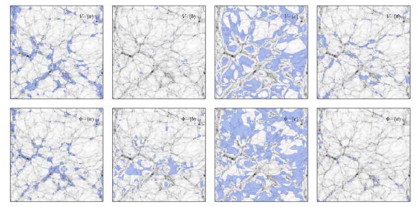
On the other hand, since the dynamical trajectories differ significantly for positive and negative $s^{(v/\phi)}_{1}$ in the invariant space, it is convenient to further divide both filament and sheet morphologies based on the sign of $s^{(v/\phi)}_{1}$. In Figure (4), we perform this detailed comparison for the same simulation snapshot as in Figure (1). Interestingly, given almost completely different structures in Figure (1), filaments with positive $s^{(v/\phi)}_{1}$, shown in the first column of the figure, exhibit a very similar pattern for both tensors. Moreover, the major contribution to the dissimilarity come from the filaments with negative $s^{(v/\phi)}_{1}$, as shown in the second column, where much more regions are classified as this type for tensor $\Phi_{ij}$ than $A_{ij}$.

Assuming the nonlinear local model, we then plot in Figure. (5) the dynamical evolution of invariants for tensors $A_{ij}$ and $-\Phi_{ij}$ together, who are indeed comparable as we have already rescaled the invariants so that $\rm tr[A_{ij}]=\rm tr[-\Phi_{ij}]=\pm 1$. For underdense perturbation $\delta_{0}<0$, one sees that morphologies from both tensors exhibit similar sheet instability, as all trajectories evolve towards the voids or filaments. Meanwhile, it is obvious that trajectories in $s^{\phi}$ space squeeze towards the boundary separating real and complex solutions. By definition, this suggests at least two of eigenvalues should be closer to each other than that of tensor $A_{ij}$. Since $\Phi_{ij}$ is simply proportional to $A_{ij}$ initially, an immediate consequence is the enrichment of potential classified filaments with negative density perturbation $\delta$, which is exactly what has been observed in the simulation.

Physically, at least two factors are responsible for such behavior, as suggested by the nonlinear local model. The first is that the angle $\beta$ approaches $\pi$ from the value of $0$ faster than $\alpha$, and therefore it would produce more filamentary structures. On the other hand, since the evolution equation of the tidal tensor (equation 3.2.1) is sourced by both density $\rho$ (instead of density perturbation $\delta$) and the shear tensor $\sigma_{ij}$, $\varepsilon_{ij}$ grows as $\varepsilon(1+\delta)$ compared with $\sigma$ for shear tensor (equation 3.2.1). Consequently, the rescaled tidal tensor $\widetilde{\varepsilon}_{ij}\propto\varepsilon(1+\delta)Q_{ij}(\beta)/|\delta|$ would grow slower than the rescaled shear tensor $\widetilde{\sigma}_{ij}\propto\sigma Q_{ij}(\alpha)/|\theta|$ for underdense perturbation $0>\delta>-1$, for in general $|\varepsilon(1+\delta)/\delta|<|\sigma/\theta|$. Therefore, the differences between eigenvalues $\Delta\lambda$ are usually narrower for tensor $\Phi_{ij}$ than $A_{ij}$. From the definition of $s^{v/\phi}_{2}$ in equation (3.2.1) and (3.2.1), this corresponds to a slower motion of invariant $s^{(\phi)}_{2}$ than $s^{(v)}_{2}$, as shown in Figure (5).

For overdense perturbation $\delta_{0}>0$, $s^{\phi}_{i}$ also evolves very differently than $s^{(v)}_{i}$. Unlike velocity invariants, where the first singularity occurs at $s^{(v)}_{2}/|s^{(v)}_{1}|^{2}\to 0$, both $s^{(\phi)}_{2}/|s^{(\phi)}_{1}|^{2}$ and $s^{(\phi)}_{3}/|s^{(\phi)}_{1}|^{3}$ approach infinity as $\varepsilon(1+\delta)/\delta\to\infty$, which again is due to the source term of the evolution equation of tidal field $\varepsilon_{ij}$. However, this does not necessarily suggest the kinematic and dynamical morphologies differ in this regime. For vanishing threshold $\lambda_{th}=0$, or even some reasonable nonzero values, clusters and sheets identified with both tensors will turn to filaments very soon so that no significant differences would emerge.

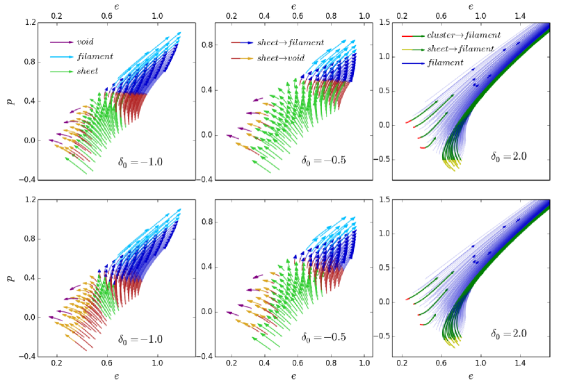
This could also be seen with the help of the evolution of deformation tensor. In Figure. (6), we plot the evolution of ellipticity $e$ and prolaticity $p$, colored by the kinematic morphologies in upper panels and dynamical categories in the lower ones. Morphological changes are characterized by segmented color arrows, with the discontinuity point reflecting the epoch of the morphology transition. The trajectories are calculated via equation (40) with $A_{ij}$ supplemented by the nonlinear local model. As expected, the overdense perturbations, shown in the third column, would evolve from various initial values towards much higher $e$ and $p$ as they become filaments. Moreover, both velocity and potential classifications display very similar morphology categorizations.

For the underdense region, we show both $\delta_{0}=-1$ and $\delta_{0}=-0.5$ in the first two columns. Consistent with the bifurcate evolution in the invariant space, trajectories with various initial ellipticity and prolaticity flow towards the opposite directions in $e-p$ plane. One is the spherical void region with $e\sim 0$ and $p\sim 0$, and the other is the non-spherical prolate filament region with $e\approx p\sim 1$, while the non-spherical sheets reside in between. Since both upper and lower panels display the same geometrical evolution of a fluid element, the color scheme shows that gravitational potential-based algorithm in general would identify more filaments and fewer sheets than kinematical classification.

4.3 Eigenvalue Threshold and the Ambiguity of Cosmic Web Definition

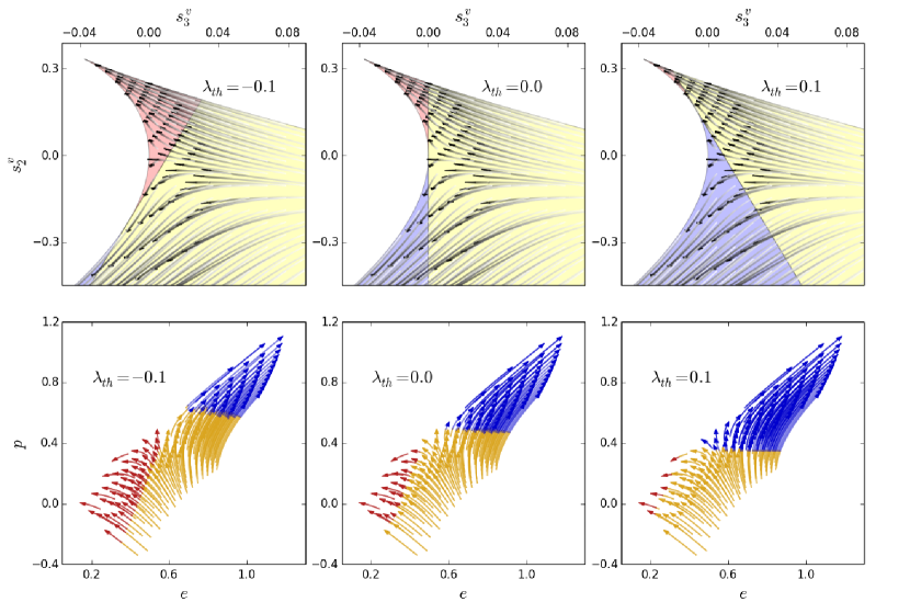
Practically, a nonzero threshold is usually applied in the algorithm to ‘optimize’ the visual impression of the cosmic web. As already shown in Figure (2), a negative $\lambda_{th}$ would indeed help to reduce the otherwise excessive filaments and sheets, meanwhile increase the volume fraction of void regions. However, geometric deformation of a fluid element is well defined by quantities like ellipticity and prolaticity. In Figure. (7), we highlight the morphologies variations in both velocity invariant space and the deformation $e-p$ plane. Since all trajectories in the upper panels are normalized by $|s^{(v)}_{1}(a)|^{n}$, where $n=(2,3)$, this corresponds to a time-dependent threshold $\lambda^{\prime}_{th}(a)=\lambda_{th}|s_{1}(a)|$ with constant $\lambda_{th}=-0.1,0$ and $0.1$ respectively. Therefore, the morphology of a fluid element with given shape measurement depends on the threshold $\lambda_{th}$, which reflects the ambiguous definition of the cosmic web.

This then leads to the question about the purpose of the morphological classification and its associated ‘best’ algorithm. An outstanding visual impression would require both density threshold and anisotropic information, like $A_{ij}$ or $\Phi_{ij}$, at various scales. For many studies, e.g. the environmental dependence of halo formation, it is probably more important to describe quantitatively the entanglement of relevant quantities than satisfying the preference of the human brain. In this sense, the ‘morphology classification’ is only a simplification to the more complicated problem. Without any arbitrary tuning of the threshold, the tensor $A_{ij}$ and $\Phi_{ij}$ themselves and corresponding rotational invariants are attractive quantities as they characterize the underlying physical processes. Therefore, besides developing various classification algorithms, more efforts should be made to understand the detailed evolution of these quantities.

5 Conclusion and Discussion

In this paper, we revisited the Lagrangian evolution of various tensors, including the velocity gradient tensor $A_{ij}$, the Hessian matrix of gravitational potential $\Phi_{ij}$ and the deformation tensor $\Psi_{ij}$, for their useful applications in the cosmic web classification. Unlike previous studies, we performed the investigation in the invariant space, defined as coefficients of the characteristic equation of $A_{ij}$ and $\Phi_{ij}$. Compared with the eigenvalue representation, this parameter space is much more convenient in tracking the dynamical evolution of these tensors. We then presented the solution for both Zel’dovich approximation and the nonlinear local model. Although the latter model is neither Newtonian nor fully general relativistic, it is reasonable to assume to be a suitable approximation for our purpose.

Since one could easily write down the analytical solution of invariants evolution in ZA, we reconfirm the fact that cosmic morphologies would not change before approaching a one-dimensional singularity in this model. However, the nonlinear local model would in general lead to the morphology instability and changes. For overdense perturbation, the sheet configurations usually collapse to filaments very quickly due to the coupling between tidal tensor $\varepsilon_{ij}$ and velocity shear $\sigma_{ij}$. For underdense regions, however, the sheet could either evolve to void or filament depending on the balance between the shear $\sigma$ and divergence $\theta$ for $A_{ij}$, or the tides $\varepsilon$ and density $\delta$ for $\Phi_{ij}$.

Interestingly, our comparison of the invariants trajectories between tensor $A_{ij}$ and $\Phi_{ij}$ suggests that different evolving speed of the instability is responsible for some distinctions of the cosmic web classified using these two tensors. Since both tensors start from the same morphologies initially, the squeezed trajectories of $\Phi_{ij}$ in Figure (5) suggests more abundant filaments with negative $s^{(\phi)}_{1}$, which is exactly what has been observed in the simulation. Physically, this is caused by both different evolving speed of tensor angle $\alpha$ and $\beta$, and the source term of the tidal field evolution equation (3.2.1).

However, there’re some limitations of our approach as well. First of all, the dynamics only work before the singularity, therefore very little conclusion would be able to make for overdense regions. Fortunately, for our purpose, it is equally, if not more, important to study the underdense perturbations. Secondly, since it’s still possible that this nonlinear local model would not fully capture the real dynamics, one need to be cautious about the direct comparison between simulation and the model calculation. For example, from Figure (5), one might also expect to observe more potential classified voids than the other algorithm. However, the simulation measurement produces somewhat similar fractions of voids for these two methods. In addition, if one tries to measure the eigenvalue differences $\Delta\lambda=|\lambda_{i}-\lambda_{j}|,~{}i\neq j$ from the simulation, the inequality

$$\Delta\lambda^{(v)}>\Delta\lambda^{(\phi)}$$ (44)

would only hold for the differences between the largest eigenvalue and the other two. For the difference between the smallest two eigenvalues, however, both tensors have similar distributions, with only slightly asymmetry favoring equation (44). On the other hand, theoretical calculation shows its validity for all three $\Delta\lambda$s. Nevertheless, whether or not this suggests the failure of the model is not clear.

References

- Aragón-Calvo et al. (2007) Aragón-Calvo M. A., Jones B. J. T., van de Weygaert R., van der Hulst J. M., 2007, A&A, 474, 315
- Avila-Reese et al. (2005) Avila-Reese V., Colín P., Gottlöber S., Firmani C., Maulbetsch C., 2005, ApJ, 634, 51
- Bernardeau, & van de Weygaert (1996) Bernardeau, F., van de Weygaert, R., 1996, MNRAS, 279, 693
- Bernardeau et al. (2002) Bernardeau, F., Colombi, S., Gaztañaga, E., Scoccimarro, R., 2002, Physical Report, 367, 1
- Bertschinger & Jain (1994) Bertschinger, E., Jain, B., 1994, APJ, 431, 486
- Bertschinger & Hamilton (1994) Bertschinger, Edmund, Hamilton, A. J. S., 1994, ApJ, 435, 1
- Bett et al. (2007) Bett P., Eke V., Frenk C. S., Jenkins A., Helly J., Navarro J., 2007, MNRAS, 376, 215
- Blanton et al. (2005) Blanton M. R., Eisenstein D., Hogg D. W., Schlegel D. J., Brinkmann J., 2005, ApJ, 629, 143
- Bond et al. (1996) Bond, J. R., Kofman, L., Pogosyan, D., 1996, Nature, 380, 603
- Bruni et al. (1995) Bruni, M., Matarrese, S., Pantano, O., 1995, APJ, 445, 958
- Chong et al. (1990) Chong, M. S., Perry, A. E., & Cantwell, B. J. 1990, Physics of Fluids, 2, 765
- Colless et al. (2003) Colless M. et al., 2003, preprint arXiv:astro-ph/0306581
- Croudace et al. (1994) Croudace, K. M., Parry, J., Salopek, D. S., Stewart, J. M., 1994, APJ, 423, 22
- de Lapparent et al. (1986) de Lapparent V., Geller M. J., Huchra J. P., 1986, ApJ, 302, L1
- Doroshkevich (1970) Doroshkevich A. G., 1970, Astrophyzika, 3, 175
- Dressler (1980) Dressler A., 1980, ApJ, 236, 351
- Ellis (1971) Ellis, G. F. R., 1971, General Relativity and Cosmology, ed. R. K. Sachs (New York: Academic), 104
- Ellis & Dunsby (1997) Ellis, G. F. R., Dunsby P. K. S., 1997, ApJ, 479, 97
- Forero-Romero et al. (2009) Forero-Romero, J. E., Hoffman, Y., Gottlöber, S., Klypin, A., Yepes, G., 2009, MNRAS, 396, 1815
- Geller & Huchra (1989) Geller M. J., Huchra J. P., 1989, Science, 246, 897
- Gregory & Thompson (1978) Gregory S. A., Thompson L. A., 1978, ApJ, 222, 784
- Hahn et al. (2007a) Hahn, O., Porciani, C., Carollo, C. M., Dekel, A., 2007, MNRAS, 375, 489
- Hahn et al. (2007b) Hahn, O., Carollo, C. M., Porciani, C., Dekel, A., 2007, MNRAS, 381, 41
- Hahn et al. (2014) Hahn, O., Angulo, R. E., Abel, T., 2014, arxiv:1404.2280
- Hoffman et al. (2012) Hoffman, Y., et al., 2012, MNRAS, 425, 2049
- Huchra et al. (2005) Huchra J., et al., 2005, In: Nearby Large-Scale Structures and the Zone of Avoidance, ASP Conf. Ser. Vol. 239, eds. K.P. Fairall, P.A. Woudt (Astron. Soc. Pac., San Francisco),p. 135
- Hui & Bertschinger (1996) Hui, Lam, Bertschinger, Edmund, 1996, ApJ, 471, 1
- Kauffmann et al. (2004) Kauffmann G., White S. D. M., Heckman T. M., Ménard B., Brinchmann J., Charlot S., Tremonti C., Brinkmann J., 2004, MNRAS, 353, 713
- Lemson & Kauffmann (1999) Lemson G., Kauffmann G., 1999, MNRAS, 302, 111
- Lesame et al. (1995) Lesame, W. M., Dunsby, P. K. S., Ellis, G. F. R., 1995, Phys. Rev. D, 52, 3406
- Lynden-Bell (1967) Lynden-Bell, D., 1967, MNRAS, 136, 101
- Macciò et al. (2007) Macciò A. V., Dutton A. A., van den Bosch F. C., Moore B., Potter D., Stadel J., 2007, MNRAS, 378, 55
- Massey et al. (2007) Massey R., Rhodes J., Ellis R., Scoville N., et al. 2007, Nature, 445, 286
- Matarrese et al. (1993) Matarrese, S., Pantano, O., Saez, D., 1993, Phys. Rev. D., 47, 1311
- Matarrese (1994) Matarrese, S., Pantano, O., Saez, D., 1994, Phys. Rev. Lett., 72, 320
- Monaco (1995) Monaco, Pierluigi, 1995, APJ, 447, 23.
- Munshi (1994) Munshi, D., Starobinski, A. A., 1994, 428, 433
- Novikov et al. (2006) Novikov D., Colombi S., Doré O., 2006, MNRAS, 366, 1201
- Schaap & van de Weygaert (2000) Schaap, W. E., van de Weygaert, R., 2000, A&A, 363, L29
- Peebles (1980) Peebles P. J. E., 1980, The large-scale structure of the universe, Peebles, P. J. E., ed.
- Pelupessy et al. (2003) Pelupessy, F. I., Schaap, W. E., van de Weygaert, R., 2003, A&A, 403, 389
- Shectman et al. (1996) Shectman S. A., Landy S. D., Oemler A., Tucker D. L., Lin H., Kirshner R. P., Schechter P. L., 1996, ApJ, 470, 172
- Sheth & Tormen (2004) Sheth R. K., Tormen G., 2004, MNRAS, 350, 1385
- Sousbie et al. (2008) Sousbie T., Pichon C., Colombi S., Novikov D., Pogosyan D., 2008, MNRAS, 383, 1655
- Tegmark et al. (2004) Tegmark M. et al., 2004, ApJ, 606, 702
- Wang et. al. (2014) Wang X., Szalay A., et. al., 2014, ApJ, 793, 58
- Wechsler et al. (2005) Wechsler R. H., Zentner A. R., Bullock J. S., Kravtsov A. V., Allgood B., 2005, ApJ, 652, 71
- Wetzel et al. (2007) Wetzel A. R., Cohn J. D., White M., Holz D. E., Warren M. S., 2007, ApJ, 656, 139
- Wilczek (2010) Wilczek M., 2010, PhD thesis, University of Münster
- Zel’dovich (1970) Zel’dovich, Ya. B., 1970, Astronomy and Astrophysics, 5, 84