Differentially Private Distributed Constrained Optimization

Abstract

Many resource allocation problems can be formulated as an optimization problem whose constraints contain sensitive information about participating users. This paper concerns solving this kind of optimization problem in a distributed manner while protecting the privacy of user information. Without privacy considerations, existing distributed algorithms normally consist in a central entity computing and broadcasting certain public coordination signals to participating users. However, the coordination signals often depend on user information, so that an adversary who has access to the coordination signals can potentially decode information on individual users and put user privacy at risk. We present a distributed optimization algorithm that preserves differential privacy, which is a strong notion that guarantees user privacy regardless of any auxiliary information an adversary may have. The algorithm achieves privacy by perturbing the public signals with additive noise, whose magnitude is determined by the sensitivity of the projection operation onto user-specified constraints. By viewing the differentially private algorithm as an implementation of stochastic gradient descent, we are able to derive a bound for the suboptimality of the algorithm. We illustrate the implementation of our algorithm via a case study of electric vehicle charging. Specifically, we derive the sensitivity and present numerical simulations for the algorithm. Through numerical simulations, we are able to investigate various aspects of the algorithm when being used in practice, including the choice of step size, number of iterations, and the trade-off between privacy level and suboptimality.

I Introduction

Electric vehicles (EVs), including pure electric and hybrid plug-in vehicles, are believed to be an important component of future power systems [16]. Studies predict that the market share of EVs in the United States can reach approximately 25% by year 2020 [12]. By that time, EVs will become a significant load on the power grid [27, 3], which can lead to undesirable effects such as voltage deviations if charging of the vehicles are uncoordinated.

The key to reducing the impact of EVs on the power grid is to coordinate their charging schedules, which is often cast as a constrained optimization problem with the objective of minimizing the peak load, power loss, or load variance [26, 5]. Due to the large number of vehicles, computing an optimal schedule for all vehicles can be very time consuming if the computation is carried out on a centralized server that collects demand information from users. Instead, it is more desirable that the computation is distributed to individual users. Among others, Ma et al. [19] proposed a distributed charging strategy based on the notion of valley-filling charging profiles, which is guaranteed to be optimal when all vehicles have identical (i.e., homogeneous) demand. Gan et al. [11] proposed a more general algorithm that is optimal for nonhomogeneous demand and allows asynchronous communication.

In order to solve the constrained optimization problem of scheduling in a distributed manner, the server is required to publish certain public information that is computed based on the tentative demand collected from participating users. Charging demand often contains private information of the users. As a simple example, zero demand from a charging station attached to a single home unit is a good indication that the home owner is away from home. Note that the public coordination signal is received by everyone including potential adversaries whose goal is to decode private user information from the public signal, so that it is desirable to develop solutions for protecting user privacy.

It has been long recognized that ad hoc solutions such as anonymization of user data are inadequate to guarantee privacy due to the presence of public side information. A famous case is the reidentification of certain users from an anonymized dataset published by Netflix, which is an American provider of on-demand Internet streaming media. The dataset was provided for hosting an open competition called the Netflix Prize for find the best algorithm to predict user ratings on films. It has been reported that certain Netflix subscribers can be identified from the anonymized Netflix prize dataset through auxiliary information from the Internet Movie Database (IMDb) [20]. As such, providing rigorous solutions to preserving privacy has become an active area of research. In the field of systems and control, recent work on privacy includes, among others, filtering of streaming data [18], smart metering [24], traffic monitoring [2], and privacy in stochastic control [29].

Recently, the notion of differential privacy proposed by Dwork and her collaborators has received attention due to its mathematically rigorous formulation [8]. The original setting assumes that the sensitive user information is held by a trustworthy party (often called curator in related literature), and the curator needs to answer external queries (about the sensitive user information) that potentially come from an adversary who is interested in learning information belonging to some user. For example, in EV charging, the curator is the central server that aggregates user information, and the queries correspond to public coordination signals. Informally, preserving differential privacy requires that the curator must ensure that the results of the queries remain approximately unchanged if data belonging to any single user are modified. In other words, the adversary should know little about any single user’s information from the results of queries. A recent survey on differential privacy can be found in [7]; there is also a recent textbook on this topic written by Dwork and Roth [9].

Contributions

Motivated by the privacy concerns in EV charging and recent advances in differential privacy, in this paper, we investigate the problem of preserving differential privacy in distributed constrained optimization. We present a differentially private distributed algorithm for solving a class of constrained optimization problems, whose privacy guarantee is proved using the adaptive composition theorem. We show that the private optimization algorithm can be viewed as an implementation of stochastic gradient descent [22]. Based on previous results on stochastic gradient descent [25], we are able to derive a bound for the suboptimality of our algorithm and reveal the trade-off between privacy and performance of the algorithm.

We illustrate the applicability of this general framework of differentially private distributed constrained optimization in the context of EV charging. To this end, we begin by computing the sensitivity of the public signal with respect to changes in private information. Specifically, this requires analyzing the sensitivity of the projection operation onto the user-specified constraints. Although such sensitivity can be difficult to compute for a general problem, using tools in optimization theory, we are able to derive an explicit expression of the sensitivity for the EV charging example. Through numerical simulations, we show that our algorithm is able to provide strong privacy guarantees with little loss in performance when the number of participating users (i.e., vehicles) is large.

Related work

There is a large body of research work on incorporating differential privacy into resource allocation problems. A part of the work deals with indivisible resources (or equivalently, games with discrete actions), including the work by, among others, Kearns et al. [17], Rogers and Roth [23], and Hsu et al. [13]. Our paper focuses on the case of divisible resources and where private information is contained in the constraints of the allocation problem.

In the work of differentially private resource allocation, it is a common theme that the coordination signals are randomly perturbed to avoid revealing private information of the users, such as in the work by Huang et al. [15] and Hsu et al. [14]. Huang et al. [15] study the problem of differentially private convex optimization in the absence of constraints. In their formulation, the private user information is encoded in the individual cost functions and can be interpreted as user preferences. Apart from incorporating constraints, a major difference of our setting compared to Huang et al. [15] is the way that privacy is incorporated into the optimization problem. In Huang et al. [15], they assume that the public coordination signals do not change when the individual cost function changes. However, this assumption fails to hold, e.g., in the case of EV charging, where the coordination signal is computed by aggregating the response from users and hence is sensitive to changes in user information. Instead, we treat the public coordination signals as the quantity that needs to be perturbed (i.e., as a query, in the nomenclature of differential privacy) in order to prevent privacy breach caused by broadcasting the signals.

The recent work by Hsu et al. [14] on privately solving linear programs is closely related to our work, since their setting also assumes that the private information is contained in the (affine) constraints. Our work can be viewed as a generalization of their setting by extending the form of objective functions and constraints. In particular, the objective function can be any convex function that depends on the aggregate allocation and has Lipschitz continuous gradients. The constraints can be any convex and separable constraints; for illustration, we show how to implement the algorithm for a particular set of affine constraints motivated by EV charging.

Paper organization

The paper is organized as follows. Section II introduces the necessary background on (non-private) distributed optimization and, in particular, projected gradient descent. Section III reviews the results in differential privacy and gives a formal problem statement of differentially private distributed constrained optimization. Section IV gives an overview of the main results of the paper. Section V describes a differentially private distributed algorithm that solves a general class of constrained optimization problems. We also study the trade-off between privacy and performance by analyzing the suboptimality of the differentially private algorithm.

In Section VI, we illustrate the implementation of our algorithm via a case study of EV charging. In particular, we compute the sensitivity of the projection operation onto user-specified constraints, which is required for implementing our private algorithm. Section VII presents numerical simulations on various aspects of the algorithm when being used in practice, including choice of step size, number of iterations, and the trade-off between privacy level and performance.

II Background: Distributed constrained optimization

II-A Notation

Denote the $\ell_{p}$-norm of any $x\in\mathbb{R}^{n}$ by $\left\|x\right\|_{p}$. The subscript $p$ is dropped in the case of $\ell_{2}$-norm. For any nonempty convex set $\mathcal{C}\subset\mathbb{R}^{n}$ and $x\in\mathbb{R}^{n}$, denote by $\Pi_{\mathcal{C}}(x)$ the projection operator that projects $x$ onto $\mathcal{C}$ in $\ell_{2}$-norm. Namely, $\Pi_{\mathcal{C}}(x)$ is the solution of the following constrained least-squares problem

$$\underset{\hat{x}}{\mathrm{min.}}\quad\|\hat{x}-x\|^{2}\qquad\;\mathrm{s.t.}\quad\hat{x}\in\mathcal{C}.$$ (1)

It can be shown that problem (1) is always feasible and has a unique solution so that $\Pi_{\mathcal{C}}$ is well-defined. For any function $f$ (not necessarily convex), denote by $\partial f(x)$ the set of subgradients of $f$ at $x$:

$$\partial f(x):=\{g\colon f(y)\geq f(x)+g^{T}(y-x)\mbox{ for all }y\}.$$

When $f$ is convex and differentiable at $x$, the set $\partial f(x)$ becomes a singleton set whose only element is the gradient $\nabla f(x)$. For any function $f$, denote its range by $\mathrm{range}(f)$. For any differentiable function $f$ that depends on multiple variables including $x$, denote by $\partial_{x}f$ the partial derivative of $f$ with respect to $x$. For any $\lambda>0$, denote by $\mathrm{Lap}(\lambda)$ the zero-mean Laplace probability distribution such that the probability density function of a random variable $X$ obeying the distribution $\mathrm{Lap}(\lambda)$ is $p_{X}(x)=\frac{1}{2\lambda}\exp(-|x|/\lambda)$. The vector consisting all ones is written as $\mathbf{1}$. The symbol $\preceq$ is used to represent element-wise inequality: for any $x,y\in\mathbb{R}^{n}$, we have $x\preceq y$ if and only if $x_{i}\leq y_{i}$ for all $1\leq i\leq n$. For any positive integer $n$, we denote by $[n]$ the set $\{1,2,\dots,n\}$.

II-B Distributed constrained optimization

Before discussing privacy issues, we first introduce the necessary background on distributed constrained optimization. We consider a constrained optimization problem over $n$ variables $r_{1},r_{2},\dots,r_{n}\in\mathbb{R}^{T}$ in the following form:

$$\underset{\{r_{i}\}_{i=1}^{n}}{\mathrm{min.}}\quad U\left({\textstyle\sum_{i=1}^{n}}r_{i}\right)$$ (2)

$$\underset{\phantom{\{r_{i}\}_{i=1}^{n}}}{\;\mathrm{s.t.}}\quad r_{i}\in\mathcal{C}_{i},\quad i\in[n].$$

Throughout the paper, we assume that the objective function $U\colon\mathbb{R}^{T}\to\mathbb{R}$ in problem (2) is differentiable and convex, and its gradient $\nabla U$ is $L$-Lipschitz in the $\ell_{2}$-norm, i.e., there exists $L>0$ such that

$$\left\|\nabla U(x)-\nabla U(y)\right\|\leq L\left\|x-y\right\|\quad\text{for all }x,y.$$

The set $\mathcal{C}_{i}$ is assumed to be convex for all $i\in[n]$. For resource allocation problems, the variable $r_{i}$ and the constraint set $\mathcal{C}_{i}$ are used to capture the allocation and constraints on the allocation for user/agent $i$.

Input: $U$, $\{\mathcal{C}_{i}\}_{i=1}^{n}$, $K$, and step sizes $\{\alpha_{k}\}_{k=1}^{K}$.

Output: $\{r_{i}^{(K+1)}\}_{i=1}^{n}$.

Initialize $\{r_{i}^{(1)}\}_{i=1}^{n}$ arbitrarily. For $k=1,2,\dots,K$, repeat:

1. Compute $p^{(k)}:=\nabla U\left({\textstyle\sum_{i=1}^{n}r_{i}^{(k)}}\right)$.

2. For $i\in[n]$, update $r_{i}^{(k+1)}$ according to

   $$r_{i}^{(k+1)}:=\Pi_{\mathcal{C}_{i}}(r_{i}^{(k)}-\alpha_{k}p^{(k)}).$$ (3)

Algorithm 1 Distributed projected gradient descent (with a fixed number of iterations).

The optimization problem (2) can be solved iteratively using projected gradient descent, which requires computation of the gradient of $U$ and its projection onto the feasible set at each iteration. The computational complexity of projected gradient descent is dominated by the projection operation and grows with $n$. For practical applications, the number $n$ can be quite large, so that it is desirable to distribute the projection operation to individual users. A distributed version of the projected gradient descent method is shown in Algorithm 1. The algorithm guarantees that the output converges to the optimal solution as $K\to\infty$ with proper choice of step sizes $\{\alpha_{k}\}_{k=1}^{K}$ (see [11] for details on how to choose $\alpha_{k}$).

III Problem formulation

III-A Privacy in distributed constrained optimization

In many applications, the specifications of $\mathcal{C}_{i}$ may contain sensitive information that user $i$ wishes to keep undisclosed from the public. In the framework of differential privacy, it is assumed that an adversary can potentially collaborate with some users in the database in order to learn about other user’s information. Under this assumption, the distributed projected descent algorithm (Algorithm 1) can lead to possible loss of privacy of participating users for reasons described below. It can be seen from Algorithm 1 that $\mathcal{C}_{i}$ affects $r_{i}^{(k)}$ through equation (3) and consequently also $p^{(k)}$. Since $p^{(k)}$ is broadcast publicly to every charging station, with enough side information (such as collaborating with some participating users), an adversary who is interested in learning private information about some user $i$ may be able to infer information about $\mathcal{C}_{i}$ from the public signals $\{p^{(k)}\}_{k=1}^{K}$. We will later illustrate the privacy issues in the context of EV charging.

III-B Differential privacy

Our goal is to modify the original distributed projected gradient descent algorithm (Algorithm 1) to preserve differential privacy. Before giving a formal statement of our problem, we first present some preliminaries on differential privacy. Differential privacy considers a set (called database) $D$ that contains private user information to be protected. For convenience, we denote by $\mathcal{D}$ the universe of all possible databases of interest. The information that we would like to obtain from a database $D$ is given by $q(D)$ for some mapping $q$ (called query) that acts on $D$. In differential privacy, preserving privacy is equivalent to hiding changes in the database. Formally, changes in a database can be defined by a symmetric binary relation between two databases called adjacency relation, which is denoted by $\mathrm{Adj}(\cdot,\cdot)$; two databases $D$ and $D^{\prime}$ that satisfy $\mathrm{Adj}(D,D^{\prime})$ are called adjacent databases.

Definition 1 (Adjacent databases).

Two databases $D=\{d_{i}\}_{i=1}^{n}$ and $D^{\prime}=\{d_{i}^{\prime}\}_{i=1}^{n}$ are said to be adjacent if there exists $i\in[n]$ such that $d_{j}=d_{j}^{\prime}$ for all $j\neq i$.

A mechanism that acts on a database is said to be differentially private if it is able to ensure that two adjacent databases are nearly indistinguishable from the output of the mechanism.

Definition 2 (Differential privacy [8]).

Given $\epsilon\geq 0$, a mechanism $M$ preserves $\epsilon$-differential privacy if for all $\mathcal{R}\subseteq\mathrm{range}(M)$ and all adjacent databases $D$ and $D^{\prime}$ in $\mathcal{D}$, it holds that

$$\mathbb{P}(M(D)\in\mathcal{R})\leq e^{\epsilon}\mathbb{P}(M(D^{\prime})\in\mathcal{R}).$$ (4)

The constant $\epsilon$ indicates the level of privacy: smaller $\epsilon$ implies higher level of privacy. The notion of differential privacy promises that an adversary cannot tell from the output of $M$ with high probability whether data corresponding to a single user in the database have changed. It can be seen that any non-constant differentially mechanism is necessarily randomized, i.e., for a given database, the output of such a mechanism obeys a certain probability distribution. Finally, although it is not explicitly mentioned in Definition 2, a mechanism needs to be an approximation of the query of interest in order to be useful. For this purpose, a mechanism is normally defined in conjunction with some query of interest; a common notation is to include the query $q$ of interest in the subscript of the mechanism as $M_{q}$.

III-C Problem formulation: Differentially private distributed constrained optimization

Recall that our goal of preserving privacy in distributed optimization is to protect the user information in $\mathcal{C}_{i}$, even if an adversary can collect all public signals $\{p^{(k)}\}_{k=1}^{K}$. To mathematically formulate our goal under the framework of differential privacy, we define the database $D$ as the set $\{\mathcal{C}_{i}\}_{i=1}^{n}$ and the query as the $K$-tuple consisting of all the gradients $p=(p^{(1)},p^{(2)},\dots,p^{(K)})$. We assume that $\mathcal{C}_{1},\mathcal{C}_{2},\dots,\mathcal{C}_{n}$ belong a family of sets parameterized by $\alpha\in\mathbb{R}^{s}$. Namely, there exists a parameterized set $\mathcal{C}$ such that for all $i\in[n]$, we can write $\mathcal{C}_{i}=\mathcal{C}(\alpha_{i})$ for some $\alpha_{i}\in\mathbb{R}^{s}$. We also assume that there exists a metric $\rho\colon\mathbb{R}^{s}\times\mathbb{R}^{s}\to\mathbb{R}_{+}$. In this way, we can define the distance $\rho_{\mathcal{C}}(\mathcal{C}_{i},\mathcal{C}_{i}^{\prime})$ between any $\mathcal{C}_{i}=\mathcal{C}(\alpha_{i})$ and $\mathcal{C}_{i}^{\prime}=\mathcal{C}(\alpha_{i}^{\prime})$ using the metric $\rho$ as

$$\rho_{\mathcal{C}}(\mathcal{C}_{i},\mathcal{C}_{i}^{\prime}):=\rho(\alpha_{i},\alpha_{i}^{\prime}).$$

For any given $\delta\mathcal{C}\in\mathbb{R}_{+}$, we define and use throughout the paper the following adjacency relation between any two databases $D$ and $D^{\prime}$ in the context of distributed constrained optimization.

Definition 3 (Adjacency relation for constrained optimization).

For any databases $D=\{\mathcal{C}_{i}\}_{i=1}^{n}$ and $D^{\prime}=\{\mathcal{C}_{i}^{\prime}\}_{i=1}^{n}$, it holds that $\mathrm{Adj}(D,D^{\prime})$ if and only if there exists $i\in[n]$ such that $\rho_{\mathcal{C}}(\mathcal{C}_{i},\mathcal{C}_{i}^{\prime})\leq\delta\mathcal{C}$, and $\mathcal{C}_{j}=\mathcal{C}_{j}^{\prime}$ for all $j\neq i$.

The constant $\delta\mathcal{C}$ is chosen based on the privacy requirement, i.e., the kind of user activities that should be kept private. Using the adjacency relation described in Definition 3, we state in the following the problem of designing a differentially private distributed algorithm for constrained optimization.

Problem 4 (Differentially private distributed constrained optimization).

Find a randomized mechanism $M_{p}$ that approximates the gradients $p=(p^{(1)},p^{(2)},\dots,p^{(K)})$ (defined in Algorithm 1) and preserves $\epsilon$-differential privacy under the adjacency relation described in Definition 3. Namely, for any adjacent databases $D$ and $D^{\prime}$, and any $\mathcal{R}\subseteq\mathrm{range}(M_{p})$, the mechanism $M_{p}$ should satisfy

$$\mathbb{P}(M_{p}(D)\in\mathcal{R})\leq e^{\epsilon}\mathbb{P}(M_{p}(D^{\prime})\in\mathcal{R}).$$

III-D Example application: EV charging

In EV charging, the goal is to charge $n$ vehicles over a horizon of $T$ time steps with minimal influence on the power grid. For simplicity, we assume that each vehicle belongs to one single user. For any $i\in[n]$, the vector $r_{i}\in\mathbb{R}^{T}$ represents the charging rates of vehicle $i$ over time. In the following, we will denote by $r_{i}(t)$ the $t$-th component of $r_{i}$. Each vehicle needs to be charged a given amount of electricity $E_{i}>0$ by the end of the scheduling horizon; in addition, for any $t\in[T]$, the charging rate $r_{i}(t)$ cannot exceed the maximum rate $\bar{r}_{i}(t)$ for some given constant vector $\bar{r}_{i}\in\mathbb{R}^{T}$. Under these constraints on $r_{i}$, the set $\mathcal{C}_{i}$ is described as follows:

$$0\preceq r_{i}\preceq\bar{r}_{i},\qquad\mathbf{1}^{T}r_{i}=E_{i}.$$ (5)

The tuple $(\bar{r}_{i},E_{i})$ is called the charging specification of user $i$. Throughout the paper, we assume that $\bar{r}_{i}$ and $E_{i}$ satisfy

$$\mathbf{1}^{T}\bar{r}_{i}\geq E_{i}\quad\text{for all }i\in[n],$$ (6)

so that the constraints (5) are always feasible.

The objective function $U$ in problem (2) quantifies the influence of a charging schedule $\{r_{i}\}_{i=1}^{n}$ on the power grid. We choose $U$ as follows for the purpose of minimizing load variance:

$$U\left({\textstyle\sum_{i=1}^{n}r_{i}}\right)=\frac{1}{2}\left\|d+{\textstyle\sum_{i=1}^{n}r_{i}}/m\right\|^{2}.$$ (7)

In (7), $m$ is the number of households, which is assumed proportional to the number of EVs, i.e., there exists $\gamma$ such that $n/m=\gamma$; then, the quantity ${\textstyle\sum_{i=1}^{n}r_{i}}/m$ becomes the aggregate EV load per household. The vector $d\in\mathbb{R}^{T}$ is the base load profile incurred by loads in the power grid other than EVs, so that $U\left({\textstyle\sum_{i=1}^{n}r_{i}}\right)$ quantifies the variation of the total load including the base load and EVs. It can be verified that $U$ is convex and differentiable, and $\nabla U$ is Lipschitz continuous.

The set $\mathcal{C}_{i}$ (defined by $\bar{r}_{i}$ and $E_{i}$) can be associated with personal activities of the owner of vehicle $i$ in the following way. For example, $\bar{r}_{i}(t)=0$ may indicate that the owner is temporarily away from the charging station (which may be co-located with the owner’s residence) so that the vehicle is not ready to be charged. Similarly, $E_{i}=0$ may indicate that the owner is not actively using the vehicle so that the vehicle does not need to be charged.

We now illustrate why publishing the exact gradient $p^{(k)}$ can potentially lead to a loss of privacy. The gradient $p^{(k)}$ can be computed as $p^{(k)}=\frac{1}{m}(d+{\textstyle\sum_{i=1}^{n}r_{i}}/m)$. If an adversary collaborates with all but one user $i$ so that the adversary is able obtain $r_{j}^{(k)}$ for all $j\neq i$ in the database. Then, the adversary can infer $r_{i}^{(k)}$ exactly from $p^{(k)}$, even though user $i$ did not reveal his $r_{i}^{(k)}$ to the adversary. After obtaining $r_{i}^{(k)}$, the adversary can obtain information on $\mathcal{C}_{i}$ by, for example, computing $E_{i}=\mathbf{1}^{T}r_{i}^{(k)}$.

The adjacency relation in the case of EV charging is defined as follows. Notice that, in the case of EV charging, the parameter $\alpha_{i}$ that parameterizes the set $\mathcal{C}_{i}$ is given by $\alpha_{i}=(\bar{r}_{i},E_{i})$, in which $(\bar{r}_{i},E_{i})$ is the charging specifications of user $i$ as defined in (5).

Definition 5 (Adjacency relation for EV charging).

For any databases $D=\{\mathcal{C}_{i}(\bar{r}_{i},E_{i})\}_{i=1}^{n}$ and $D^{\prime}=\{\mathcal{C}_{i}^{\prime}(\bar{r}_{i}^{\prime},E_{i}^{\prime})\}_{i=1}^{n}$, we have $\mathrm{Adj}(D,D^{\prime})$ if and only if there exists $i\in[n]$ such that

$$\left\|\bar{r}_{i}-\bar{r}_{i}^{\prime}\right\|_{1}\leq\delta r,\qquad|E_{i}-E_{i}^{\prime}|\leq\delta E,$$ (8)

and $\bar{r}_{j}=\bar{r}_{j}^{\prime}$, $E_{j}=E_{j}^{\prime}$ for all $j\neq i$.

In terms of choosing $\delta E$ and $\delta r$, one useful choice for $\delta E$ is the maximum amount of energy an EV may need; this choice of $\delta E$ can be used to hide the event corresponding to whether an user needs to charge his vehicle.

IV Overview of main results

IV-A Results for general constrained optimization problems

Input: $U$, $L$, $\{\mathcal{C}_{i}\}_{i=1}^{n}$, $K$, $\{\alpha_{k}\}_{k=1}^{K}$, $\eta\geq 1$, $\Delta$, and $\epsilon$.

Output: $\{\hat{r}_{i}^{(K+1)}\}_{i=1}^{n}$.

Initialize $\{r_{i}^{(1)}\}_{i=1}^{n}$ arbitrarily. Let $\hat{r}_{i}^{(1)}=r_{i}^{(1)}$ for all $i\in[n]$ and $\theta_{k}=(\eta+1)/(\eta+k)$ for $k\in[K]$.

For $k=1,2,\dots,K$, repeat:

1. If $k=1$, then set $w_{k}=0$; else draw a random vector $w_{k}\in\mathbb{R}^{T}$ from the distribution (proportional to) $\exp\left(-\frac{2\epsilon\left\|w_{k}\right\|}{K(K-1)L\Delta}\right)$

2. Compute $\hat{p}^{(k)}:=\nabla U\left({\textstyle\sum_{i=1}^{n}r_{i}^{(k)}}\right)+w_{k}$.

3. For $i\in[n]$, compute:

   $$r_{i}^{(k+1)} :=\Pi_{\mathcal{C}_{i}}(r_{i}^{(k)}-\alpha_{k}\hat{p}^{(k)}),$$

   $$\hat{r}_{i}^{(k+1)} :=(1-\theta_{k})\hat{r}_{i}^{(k)}+\theta_{k}r_{i}^{(k+1)}.$$

Algorithm 2 Differentially private distributed projected gradient descent.

In the first half of the paper, we present the main algorithmic result of this paper, a differentially private distributed algorithm (Algorithm 2) for solving the constrained optimization problem (2). The constant $\Delta$ that appears in the input of Algorithm 2 is defined as

$$\Delta:=\max_{i\in[n]}\max\Bigl{\{}\left\|\Pi_{\mathcal{C}_{i}}(r)-\Pi_{\mathcal{C}_{i}^{\prime}}(r)\right\|\colon\\ r\in\mathbb{R}^{T},\ \mathcal{C}_{i}\text{ and }\mathcal{C}_{i}^{\prime}\text{ satisfy }\rho_{\mathcal{C}}(\mathcal{C}_{i},\mathcal{C}_{i}^{\prime})\leq\delta\mathcal{C}\Bigr{\}}.$$ (9)

In other words, $\Delta$ can be viewed as a bound on the global $\ell_{2}$-sensitivity of the projection operator $\Pi_{\mathcal{C}_{i}}$ to changes in $\mathcal{C}_{i}$ for all $i\in[n]$. Later, we will illustrate how to compute $\Delta$ using the case of EV charging.

Compared to the (non-private) distributed algorithm (Algorithm 1), the key difference in Algorithm 2 is the introduction of random perturbations in the gradients (step 2) that convert $p^{(k)}$ into a noisy gradient $\hat{p}^{(k)}$. The noisy gradients $(\hat{p}^{(1)},\hat{p}^{(2)},\dots,\hat{p}^{(K)})$ can be viewed as a randomized mechanism $M_{p}$ that approximates the original gradients $p=(p^{(1)},p^{(2)},\dots,p^{(K)})$. In Section V, we will prove that the noisy gradients (as a mechanism) $M_{p}:=(\hat{p}^{(1)},\hat{p}^{(2)},\dots,\hat{p}^{(K)})$ preserve $\epsilon$-differential privacy and hence solve Problem 4.

Theorem 6.

Algorithm 2 ensures that $M_{p}:=(\hat{p}^{(1)},\hat{p}^{(2)},\dots,\hat{p}^{(K)})$ preserves $\epsilon$-differential privacy under the adjacency relation given by Definition 3.

Algorithm 2 can be viewed as an instance of stochastic gradient descent that terminates after $K$ iterations. We will henceforth refer to Algorithm 2 as differentially private distributed projected gradient descent. The step size $\alpha_{k}$ is chosen as $\alpha_{k}=c/\sqrt{k}$ for some $c>0$. The purpose of the additional variables $\{\hat{r}_{i}^{(k)}\}_{k=1}^{K}$ is to implement the polynomial-decay averaging method in order to improve the convergence rate, which is a common practice in stochastic gradient descent [25]; introducing $\{\hat{r}_{i}^{(k)}\}_{k=1}^{K}$ does not affect privacy. The parameter $\eta\geq 1$ is used for controlling the averaging weight $\theta_{k}$. Details on choosing $\eta$ can be found in Shamir and Zhang [25].

Like most iterative optimization algorithms, stochastic gradient descent only converges in a probabilistic sense as the number of iterations $K\to\infty$. In practice, the number of iterations is always finite, so that it is desirable to analyze the suboptimality for a finite $K$. In Section V, we provide an analysis on the expected suboptimality of Algorithm 2.

Theorem 7.

The expected suboptimality of Algorithm 2 after $K$ iterations is bounded as follows:

$$\mathbb{E}\left[U\left({\textstyle\sum_{i=1}^{n}\hat{r}_{i}^{(K+1)}}\right)-U^{*}\right]\\ \qquad\leq\mathcal{O}\left(\eta\sqrt{n}\rho\left(\frac{G}{\sqrt{K}}+\frac{\sqrt{2}TK^{3/2}L\Delta}{2\epsilon}\right)\right),$$ (10)

where $U^{*}$ is the optimal value of problem (2), and

$$\rho =\max\left\{\sqrt{{\textstyle\sum_{i=1}^{n}}\left\|r_{i}\right\|^{2}}\colon r_{i}\in\mathcal{C}_{i},\ i\in[n]\right\},$$

$$G =\max\{\|\nabla U\left({\textstyle\sum_{i=1}^{n}r_{i}}\right)\|\colon r_{i}\in\mathcal{C}_{i},\ i\in[n]\}.$$

IV-B Results for the case of EV charging

Having presented and analyzed the algorithm for a general distributed constrained optimization problem, in the second half of the paper, we illustrate how Algorithm 2 can be applied to the case of EV charging. In Section VI, we demonstrate how to compute $\Delta$ using the case of EV charging as an example. We show that $\Delta$ can be bounded by $\delta r$ and $\delta E$ that appear in (8) as described below.

Theorem 8.

Consider the example of EV charging (as described in Section III-D). For any $i\in[n]$, the global $\ell_{2}$-sensitivity of the projection operator $\Pi_{\mathcal{C}_{i}(\bar{r}_{i},E_{i})}$ with respect to changes in $(\bar{r}_{i},E_{i})$ is bounded by

$$\Delta\leq 2\delta r+\delta E,$$

where $\delta r$ and $\delta E$ are specified in the adjacency relation given by (8).

The suboptimality analysis given in Theorem 7 can be further refined in the case of EV charging. The special form of $U$ given by (7) allows obtaining an upper bound on suboptimality as given in Corollary 9 below.

Corollary 9.

For the cost function $U$ given by (7), the expected suboptimality of Algorithm 2 is bounded as follows:

$$\mathbb{E}\left[U\left({\textstyle\sum_{i=1}^{n}\hat{r}_{i}^{(K+1)}}\right)-U^{*}\right]\leq\mathcal{O}\left(\eta T{}^{1/4}(\Delta/n\epsilon)^{1/4}\right).$$ (11)

This upper bound shows the trade-off between privacy and performance. As $\epsilon$ decreases, more privacy is preserved but at the expense of increased suboptimality. On the other hand, this increase in suboptimality can be mitigated by introducing more participating users (i.e., by increasing $n$), which coincides with the common intuition that it is easier to achieve privacy as the number of users $n$ increases.

V Differentially private distributed projected gradient descent

In this section, we give the proof that the modified distributed projected gradient descent algorithm (Algorithm 2) preserves $\epsilon$-differential privacy. In the proof, we will extensively use results from differential privacy such as the Laplace mechanism and the adaptive sequential composition theorem.

V-A Review: Results from differential privacy

The introduction of additive noise in step 2 of Algorithm 2 is based on a variant of the widely used Laplace mechanism in differential privacy. The Laplace mechanism operates by introducing additive noise according to the $\ell_{p}$-sensitivity ($p\geq 1$) of a numerical query $q\colon\mathcal{D}\to\mathbb{R}^{m}$ (for some dimension $m$), which is defined as follows.

Definition 10 ($\ell_{p}$-sensitivity).

For any query $q\colon\mathcal{D}\to\mathbb{R}^{m}$, the $\ell_{p}$-sensitivty of $q$ under the adjacency relation $\mathrm{Adj}$ is defined as

$$\Delta_{q}:=\max\{\left\|q(D)-q(D^{\prime})\right\|_{p}\colon$$

$$\qquad D,D^{\prime}\in\mathcal{D}\text{ s.t. }\mathrm{Adj}(D,D^{\prime})\}.$$

Note that the $\ell_{p}$-sensitivity of $q$ does not depend on a specific database $D$. In this paper, we will use the Laplace mechanism for bounded $\ell_{2}$-sensitivity.

Proposition 11 (Laplace mechanism [8]).

Consider a query $q\colon\mathcal{D}\to\mathbb{R}^{m}$ whose $\ell_{2}$-sensitivity is $\Delta_{q}$. Define the mechanism $M_{q}$ as $M_{q}(D):=q(D)+w$, where $w$ is an $m$-dimensional random vector whose probability density function is given by $p_{w}(w)\propto\exp(-\epsilon\left\|w\right\|/\Delta_{q})$. Then, the mechanism $M_{q}$ preserves $\epsilon$-differential privacy.

As a basic building block in differential privacy, the Laplace mechanism allows construction of the differentially private distributed projected gradient descent algorithm described in Algorithm 2 through adaptive sequential composition.

Proposition 12 (Adaptive seqential composition [9]).

Consider a sequence of mechanisms $\{M_{k}\}_{k=1}^{K}$, in which the output of $M_{k}$ may depend on $M_{1},M_{2},\dots,M_{k-1}$ as described below:

$$M_{k}(D)=M_{k}(D,M_{1}(D),M_{2}(D),\dots,M_{k-1}(D)).$$

Suppose $M_{k}(\cdot,a_{1},a_{2},\dots,a_{k-1})$ preserves $\epsilon_{k}$-differential privacy for any $a_{1}\in\mathrm{range}(M_{1}),\dots,a_{k-1}\in\mathrm{range}(M_{k-1}).$ Then, the $K$-tuple mechanism $M:=(M_{1},M_{2},\dots,M_{K})$ preserves $\epsilon$-differential privacy for $\epsilon=\sum_{k=1}^{K}\epsilon_{k}$.

V-B Proof on that Algorithm 2 preserves $\epsilon$-differential privacy

Using the adaptive sequential composition theorem, we can show that Algorithm 2 preserves $\epsilon$-differential privacy. We can view the $K$-tuple mechanism $M_{p}:=(\hat{p}^{(1)},\hat{p}^{(2)},\dots,\hat{p}^{(K)})$ as a sequence of mechanisms $\{\hat{p}^{(k)}\}_{k=1}^{K}$. The key is to compute the $\ell_{2}$-sensitivity of $p^{(k)}:=\nabla U\left({\textstyle\sum_{i=1}^{n}r_{i}^{(k)}}\right)$, denoted by $\Delta^{(k)}$, when the outputs of $\hat{p}^{(1)},\hat{p}^{(2)},\dots,\hat{p}^{(k-1)}$ are given, so that we can obtain a differentially private mechanism $\hat{p}^{(k)}$ by applying the Laplace mechanism on $p^{(k)}$ according to $\Delta^{(k)}$.

Lemma 13.

In Algorithm 2, when the outputs of $\hat{p}^{(1)},\hat{p}^{(2)},\dots,\hat{p}^{(k-1)}$ are given, the $\ell_{2}$-sensitivity of $p^{(k)}:=\nabla U\left({\textstyle\sum_{i=1}^{n}r_{i}^{(k)}}\right)$ satisfies $\Delta^{(k)}=(k-1)L\Delta$.

Proof:

See Appendix A. ∎

With Lemma 13 at hand, we now show that Algorithm 2 preserves $\epsilon$-differential privacy (Theorem 6, Section IV).

Proof:

(of Theorem 6) For any $k\in[K]$, when the outputs of $\hat{p}^{(1)},\hat{p}^{(2)},\dots,\hat{p}^{(k-1)}$ are given, we know from Proposition 11 that $\hat{p}^{(k)}$ preserves $\epsilon_{k}$-differential privacy, where $\epsilon_{k}$ satisfies $\epsilon_{1}=0$ and for $k>1$,

$$\epsilon_{k}/\Delta^{(k)}=\frac{2\epsilon}{K(K-1)L\Delta}.$$

Use the expression of $\Delta^{(k)}$ from Lemma 13 to obtain

$$\epsilon_{k}=\frac{2(k-1)\epsilon}{K(K-1)}.$$

Using the adaptive sequential composition theorem, we know that the privacy of $M_{p}:=(\hat{p}^{(1)},\hat{p}^{(2)},\dots,\hat{p}^{(K)})$ is given by $\sum_{k=1}^{K}\epsilon_{k}=\frac{2\epsilon}{K(K-1)}\sum_{k=1}^{K}(k-1)=\epsilon$, which completes the proof. ∎

V-C Suboptimality analysis: Privacy-performance trade-off

As a consequence of preserving privacy, we only have access to noisy gradients $\{\hat{p}^{(k)}\}_{k=1}^{K}$ rather than the exact gradients $\{p^{(k)}\}_{k=1}^{K}$. Recall that the additive noise $w_{k}$ in step 2 of Algorithm 2 has zero mean. In other words, the noisy gradient $\hat{p}^{(k)}$ is an unbiased estimate of $p^{(k)}$, which allows us to view Algorithm 2 as an instantiation of stochastic gradient descent. As we mentioned in Section IV, it is in fact a variant of stochastic gradient descent that uses polynomial-decay averaging for better convergence. The stochastic gradient descent method (with polynomial-decay averaging), which is described in Algorithm 3, can be used for solving the following optimization problem:

$$\underset{x}{\mathrm{min.}}\quad f(x)\qquad\;\mathrm{s.t.}\quad x\in\mathcal{X},$$

where $x\in\mathbb{R}^{m}$ and $\mathcal{X}\subset\mathbb{R}^{m}$ for certain dimensions $m$. Proposition 14 (due to Shamir and Zhang [25]) gives an upper bound of the expected suboptimality after finitely many steps for the stochastic gradient descent algorithm (Algorithm 3).

Input: $f$, $\mathcal{X}$, $K$, $\{\alpha_{k}\}_{k=1}^{K}$, and $\eta\geq 1$.

Output: $\hat{x}^{(K+1)}$.

Initialize $x^{(1)}$ and $k=1$. Let $\hat{x}^{(1)}=x^{(1)}$ and $\theta_{k}=(\eta+1)/(\eta+k)$ for $k\in[K]$.

For $k=1,2,\dots,K$, repeat:

1. Compute an unbiased subgradient $\hat{g}_{k}$ of $f$ at $x^{(k)}$, i.e., $\mathbb{E}[\hat{g}_{k}]\in\partial f(x^{(k)})$.

2. Update $x^{(k+1)}:=\Pi_{\mathcal{X}}(x^{(k)}-\alpha_{k}\hat{g}_{k})$ and $\hat{x}^{(k+1)}:=(1-\theta_{k})\hat{x}^{(k)}+\theta_{k}x^{(k+1)}$.

Algorithm 3 Stochastic gradient descent with polynomial-decay averaging.

Proposition 14 (Shamir and Zhang [25]).

Suppose $\mathcal{X}\subset\mathbb{R}^{m}$ is a convex set and $f\colon\mathbb{R}^{m}\to\mathbb{R}$ is a convex function. Assume that there exist $\rho$ and $\widehat{G}$ such that $\sup_{x,x^{\prime}\in\mathcal{X}}\left\|x-x^{\prime}\right\|\leq\rho$ and $\max_{1\leq k\leq K}\mathbb{E}\left\|\hat{g}_{k}\right\|^{2}\leq\widehat{G}^{2}$ for $\{\hat{g}_{k}\}_{k=1}^{K}$ given by step 1 of Algorithm 3. If the step sizes are chosen as $\alpha_{k}=c/\sqrt{k}$ for some $c>0$ , then for any $K>1$, it holds that

$$\mathbb{E}(f(\hat{x}^{(K+1)})-f^{*})\leq\mathcal{O}\left(\frac{\eta(\rho^{2}/c+c\widehat{G}^{2})}{\sqrt{K}}\right),$$ (12)

where $f^{*}=\inf_{x\in\mathcal{X}}f(x)$.

A tighter upper bound can be obtained from (12) by optimizing the right-hand side of (12) over the constant $c$.

Corollary 15.

Under the same setting as Proposition 14, the suboptimality bound for Algorithm 3 is given by

$$\mathbb{E}(f(\hat{x}^{(K+1)})-f^{*})\leq\mathcal{O}\left(\eta\frac{\rho\widehat{G}}{\sqrt{K}}\right),$$ (13)

which is achieved by choosing $c=\rho/\widehat{G}$.

By applying Corollary 15, we are able obtain the bound of suboptimality for Algorithm 2 as given by Theorem 7.

Proof:

(of Theorem 7) In order to apply Corollary 15, we need to compute $\rho$ and $\widehat{G}$ for Algorithm 2. The constant $\rho$ can be obtained as

$$\rho=\max\left\{\sqrt{{\textstyle\sum_{i=1}^{n}}\left\|r_{i}\right\|^{2}}\colon r_{i}\in\mathcal{C}_{i},\ i\in[n]\right\}.$$

Recall that the definition of $\widehat{G}$ is given by $\widehat{G}^{2}:=\max_{k}\mathbb{E}\left\|\hat{g}_{k}\right\|^{2}$. It can be verified that the gradient $\hat{g}_{k}$ of the objective function $U\left({\textstyle\sum_{i=1}^{n}r_{i}^{(k)}}\right)$ with respective to $(r_{1}^{(k)},r_{2}^{(k)},\dots,r_{n}^{(k)})$ is given by $\hat{g}_{k}=[\hat{p}^{(k)},\hat{p}^{(k)},\dots,\hat{p}^{(k)}]$, which is formed by repeating $\hat{p}^{(k)}$ for $n$ times, so that we have $\widehat{G}^{2}=n\cdot\max_{k}\mathbb{E}\left\|\hat{p}^{(k)}\right\|^{2}$. Using the expression of $\hat{p}^{(k)}$, we have

$$\widehat{G} =\sqrt{n}\cdot\max_{k\in[K]}\sqrt{\left\|p^{(k)}\right\|^{2}+\mathbb{E}\left\|w_{k}\right\|^{2}}$$

$$\leq\sqrt{n}\cdot\max_{k\in[K]}\left\{\|p^{(k)}\|+\sqrt{\mathbb{E}\left\|w_{k}\right\|^{2}}\right\}$$

$$\leq\sqrt{n}(G+\sqrt{2}TK^{2}L\Delta/2\epsilon),$$

where in the last step we have used the fact that

$$\mathbb{E}\left\|w_{k}\right\|^{2} =\mathrm{var}\left\|w_{k}\right\|^{2}+\left(\mathbb{E}\left\|w_{k}\right\|\right)^{2}$$

$$=T(\Delta^{(k)}/\epsilon_{k})^{2}+T^{2}(\Delta^{(k)}/\epsilon_{k})^{2}$$

$$\leq 2T^{2}(\Delta^{(k)}/\epsilon_{k})^{2}$$

and

$$\Delta^{(k)}/\epsilon_{k}=\frac{K(K-1)L\Delta}{2\epsilon}\leq\frac{K^{2}L\Delta}{2\epsilon}.$$

Substitute the expression of $\widehat{G}$ into (13) to obtain the result. ∎

As $K$ increases, the first term in (10) decreases, whereas the second term in (10) increases. It is then foreseeable that there exists an optimal choice of $K$ that minimizes the expected suboptimality.

Corollary 16.

The expected suboptimality of Algorithm 2 is bounded as follows:

$$\mathbb{E}\left[U\left({\textstyle\sum_{i=1}^{n}\hat{r}_{i}^{(K+1)}}\right)-U^{*}\right]\\ \leq\mathcal{O}\left(\eta T{}^{1/4}n^{1/2}\rho(G^{3}L\Delta/\epsilon)^{1/4}\right),$$ (14)

where $U^{*}$, $\rho$, and $G$ are given by Theorem 7. The bound (10) is achieved by choosing $K=(\sqrt{2}G\epsilon/3TL\Delta)^{1/2}$.

Proof:

The result can be obtained by optimizing the right-hand side of (10) over $K$. ∎

However, since it is generally impossible to obtain a tight bound for $\rho$ and $\widehat{G}$, optimizing $K$ according to Corollary 16 usually does not give the best $K$ in practice; numerical simulation is often needed in order to find the best $K$ for a given problem. We will demonstrate how to choose $K$ optimally later using numerical simulations in Section VII.

VI Sensitivity computation: The case of EV charging

So far, we have shown that Algorithm 2 (specifically, the mechanism $M_{p}$ consisting of the gradients $(\hat{p}^{(1)},\hat{p}^{(2)},\dots,\hat{p}^{(K)})$ that are broadcast to every participating user) preserves $\epsilon$-differential privacy. The magnitude of the noise $w_{k}$ introduced to the gradients depends on $\Delta$, which is the sensitivity of the projection operator $\Pi_{\mathcal{C}_{i}}$ as defined in (9). In order to implement Algorithm 2, we need to compute $\Delta$ explicitly. In the next, we will illustrate how to compute $\Delta$ using the case of EV charging as an example. We will give an expression for $\Delta$ that depends on the constants $\delta r$ and $\delta E$ appearing in the adjacency relation (8). Since $\delta r$ and $\delta E$ are part of the privacy requirement, one can choose $\Delta$ accordingly once the privacy requirement has been determined.

VI-A Overview

The input of Algorithm 2 includes the constant $\Delta$ as described by (9), which bounds the global $\ell_{2}$-sensitivity of the projection operator $\Pi_{\mathcal{C}_{i}(\bar{r}_{i},E_{i})}$ with respect to changes in $(\bar{r}_{i},E_{i})$. In this section, we will derive an explicit expression of $\Delta$ for the case of EV charging. Using tools in sensitivity analysis of optimization problems, we are able to establish the relationship between $\Delta$ and the constants $\delta r$ and $\delta E$ that appear in the adjacency relation (8) used in EV charging.

Recall that for any $r\in\mathbb{R}^{T}$, the output of the projection operation $\Pi_{\mathcal{C}_{i}(\bar{r}_{i},E_{i})}(r)$ is the optimal solution to the constrained least-squares problem

$$\underset{r_{i}}{\mathrm{min.}}\quad \frac{1}{2}\|r_{i}-r\|^{2}$$ (15)

$$\;\mathrm{s.t.}\quad 0\preceq r_{i}\preceq\bar{r}_{i},\qquad\mathbf{1}^{T}r_{i}=E_{i}.$$

Define the $\ell_{2}$-sensitivity for a fixed $r$ as

$$\Delta_{r}:=\max_{i\in[n]}\max\Bigl{\{}\left\|\Pi_{\mathcal{C}_{i}(\bar{r}_{i}.E_{i})}(r)-\Pi_{\mathcal{C}_{i}(\bar{r}_{i}^{\prime},E_{i}^{\prime})}(r)\right\|\colon\\ (\bar{r}_{i},E_{i})\text{ and }(\bar{r}_{i}^{\prime},E_{i}^{\prime})\text{ satisfy }\eqref{eq:adj_ev}\Bigr{\}};$$

it can be verified that $\Delta=\max_{r\in\mathbb{R}^{T}}\Delta_{r}$. In the following, we will establish the relationship between $\Delta_{r}$ and $(\delta r,\delta E)$; we will also show that $\Delta_{r}$ does not depend on the choice of $r$, so that $\Delta=\Delta_{r}$ for any $r\in\mathbb{R}^{T}$. For notational convenience, we consider the following least-squares problem:

$$\underset{x}{\mathrm{min.}}\quad \frac{1}{2}\|x-x_{0}\|^{2}$$ (16)

$$\;\mathrm{s.t.}\quad 0\preceq x\preceq a,\qquad\mathbf{1}^{T}x=b,$$

where $x_{0}$, $a$, and $b$ are given constants. If we let

$$x_{0}=r_{0},\qquad a=\bar{r}_{i},\qquad b=E_{i},$$

then problem (16) is mapped back to problem (15). We also have $\mathbf{1}^{T}a\geq b$ based on the assumption as described in (6). Denote the optimal solution of problem (16) by $x^{*}(a,b)$. Since our purpose is to derive an expression for $\Delta_{r}$ when $r$ is fixed, we also treat $x_{0}$ as fixed and has dropped the dependence of $x^{*}$ on $x_{0}$. Our goal is to bound the global solution sensitivity with respect to changes in $a$ and $b$, i.e.,

$$\left\|x^{*}(a^{\prime},b^{\prime})-x^{*}(a,b)\right\|,$$ (17)

for any $(a,b)$ and $(a^{\prime},b^{\prime})$. We will proceed by first bounding the local solution sensitivities $\partial_{a}x^{*}$ and $\partial_{b}x^{*}$ with respect to $a$ and $b$. Then, we will obtain a bound on the global solution, sensitivity (17) through integration of $\partial_{a}x^{*}$ and $\partial_{b}x^{*}$.

VI-B Local solution sensitivity of nonlinear optimization problems

We begin by reviewing existing results on computing local solution sensitivity of nonlinear optimization problems. Consider a generic nonlinear optimization problem parametrized by $\theta\in\mathbb{R}$ described as follows:

$$\underset{x\in\mathbb{R}^{n}}{\mathrm{min.}}\quad f(x;\theta)$$ (18)

$$\;\mathrm{s.t.}\quad g_{i}(x;\theta)\leq 0,\quad i\in[p]$$

$$h_{j}(x;\theta)=0,\quad j\in[q],$$

whose Lagrangian can be expressed as

$$L(x,\lambda,\nu;\theta)=f(x;\theta)+\sum_{i=1}^{p}\lambda_{i}g_{i}(x;\theta)+\sum_{j=1}^{q}\nu_{j}h_{j}(x;\theta),$$

where $\lambda$ and $\nu$ are the Lagrange multipliers associated with constraints $\{g_{i}\}_{i=1}^{p}$ and $\{h_{j}\}_{j=1}^{q}$, respectively. If there exists a set $\Theta\subset\mathbb{R}$ such that the optimal solution is unique for all $\theta\in\Theta$, then the optimal solution of problem (18) can be defined as a function $x^{*}\colon\Theta\to\mathbb{R}^{n}$. This condition on the uniqueness of optimal solution holds for problem (16), since the objective function therein is strictly convex.

Denote by $\lambda^{*}$ and $\nu^{*}$ the optimal Lagrange multipliers. Under certain conditions described in Proposition 17 below, the partial derivatives $\partial_{\theta}x^{*}$, $\partial_{\theta}\lambda^{*}$, and $\partial_{\theta}\nu^{*}$ exist; these partial derivatives will also be referred to as local solution sensitivity of problem (18).

Proposition 17 (Fiacco [10]).

Let $(x^{*},\lambda^{*},\nu^{*})$ be the primal-dual optimal solution of problem (18). Suppose the following conditions hold.

1. $x^{*}$ is a locally unique optimal primal solution.

2. The functions $f$, $\{g_{i}\}_{i=1}^{p},$ and $\{h_{j}\}_{j=1}^{q}$ are twice continuously differentiable in $x$ and differentiable in $\theta$.

3. The gradients $\{\nabla g_{i}(x^{*})\colon g_{i}(x^{*})=0,\>i\in[p]\}$ of the active constraints and the gradients $\{\nabla h_{j}(x^{*})\colon j\in[q]\}$ are linearly independent.

4. Strict complementary slackness holds: $\lambda_{i}^{*}>0$ when $g_{i}(x^{*},\theta)=0$ for all $i\in[p]$.

Then the local sensitivity $(\partial_{\theta}x^{*},\partial_{\theta}\lambda^{*},\partial_{\theta}\nu^{*})$ of problem (18) exists and is continuous in a neighborhood of $\theta$. Moreover, $(\partial_{\theta}x^{*},\partial_{\theta}\lambda^{*},\partial_{\theta}\nu^{*})$ is uniquely determined by the following:

$$\nabla^{2}L\cdot\partial_{\theta}x^{*}+\sum_{i=1}^{p}\nabla g_{i}\cdot\partial_{\theta}\lambda_{i}^{*}+\sum_{j=1}^{q}\nabla h_{j}\cdot\partial_{\theta}\nu_{j}^{*}+\partial_{\theta}(\nabla L)=0$$

and

$$\lambda_{i}\nabla g_{i}\cdot\partial_{\theta}x^{*}+g_{i}\partial_{\theta}\lambda_{i}^{*}+\lambda_{i}^{*}\partial_{\theta}g_{i} =0,\quad i\in[p]$$

$$\nabla h_{j}\cdot\partial_{\theta}x^{*}+\partial_{\theta}h_{j} =0,\quad j\in[q].$$

VI-C Solution sensitivity of the distributed EV charging problem

We begin by computing the local solution sensitivities $\partial_{a}x^{*}$ and $\partial_{b}x^{*}$ for problem (16) using Proposition 17. After $\partial_{a}x^{*}$ and $\partial_{b}x^{*}$ are obtained, the global solution sensitivity (17) can be obtained through integration of the local sensitivity. For convenience, we compute the global solution sensitivity in $a$ and $b$ separately and combine the results in the end in the proof of Theorem 8.

One major difficulty in applying Proposition 17 is that it requires strict complementary slackness, which unfortunately does not hold for all values of $a$ and $b$. We will proceed by deriving the local solution sensitivities assuming that strict complementary slackness holds. Later, we will show that strict complementary slackness only fails at finitely many locations on the integration path, so that the integral remains unaffected.

We shall proceed by computing the solution sensitivity for $a$ and $b$ separately. First of all, we assume that $a$ is fixed and solve for the global solution sensitivity of $x^{*}$ in $b$, defined as

$$\left\|x^{*}(a,b^{\prime})-x^{*}(a,b)\right\|.$$ (19)

When strict complementary slackness holds, the following lemma gives properties of the local solution sensitivity of problem (16) with respect to $b$.

Lemma 18 (Local solution sensitivity in $b$).

When strict complementary slackness holds, the local solution sensitivity $\partial_{b}x^{*}$ of problem (16) satisfies

$$\partial_{b}x^{*}\succeq 0\qquad\text{and}\qquad\mathbf{1}^{T}\partial_{b}x^{*}=1.$$

Proof:

See Appendix B-A. ∎

The following lemma shows that the condition is only violated for a finite number of values of $b$, so that it will still be possible to obtain the global sensitivity (19) through integration.

Lemma 19.

The set of possible values of $b$ in problem (16) for which strict complementary slackness fails to hold is finite.

Proof:

See Appendix B-B. ∎

The implication of Lemma 19 is that the local solution sensitivity $\partial_{b}x^{*}$ exists everywhere except at finitely many location. It is also possible to show that the optimal solution $x^{*}(a,b)$ is continuous in $b$ (cf. Berge [1, page 116], Dantzig et al. [4], or Tropp et al. [28, Appendix I]); the continuity of $x^{*}(a,b)$ in $b$ and together with Lemma 19 imply that $\partial_{b}x^{*}$ is Riemann integrable so that we can obtain the global solution sensitivity through integration.

Proposition 20 (Global solution sensivitity in $b$).

For any $a$, $b$ and $b^{\prime}$ that satisfy $\mathbf{1}^{T}a\geq b$ and $\mathbf{1}^{T}a\geq b^{\prime}$, we have

$$\left\|x^{*}(a,b^{\prime})-x^{*}(a,b)\right\|_{1}=|b^{\prime}-b|.$$

Proof:

Without loss of generality, assume $b^{\prime}>b$. Since $x^{*}(a,b)$ is continuous in $b$, and the partial derivative $\partial_{b}x^{*}$ exists except at finitely many points according to Lemma 19, we know that $\partial_{b}x_{i}^{*}$ is Riemann integrable for all $i\in[T]$, so that

$$x_{i}^{*}(a,b^{\prime})-x_{i}^{*}(a,b)=\int_{b}^{b^{\prime}}\partial_{b}x_{i}^{*}(a,b)\,db$$

according to the fundamental theorem of calculus. Using the fact $\partial_{b}x_{i}^{*}\geq 0$ as given by Lemma 18, we have

$$x_{i}^{*}(a,b^{\prime})-x_{i}^{*}(a,b)\geq 0.$$

Then, we have

$$\left\|x^{*}(a,b^{\prime})-x^{*}(a,b)\right\|_{1}=\sum_{i=1}^{T}|x_{i}^{*}(a,b^{\prime})-x_{i}^{*}(a,b)|\\ =\sum_{i=1}^{T}(x_{i}^{*}(a,b^{\prime})-x_{i}^{*}(a,b))=\int_{b}^{b^{\prime}}\mathbf{1}^{T}\partial_{b}x^{*}(a,b)\,db.$$

Using the fact $\mathbf{1}^{T}\partial_{b}x^{*}=1$ given by Lemma 18, we obtain

$$\left\|x^{*}(a,b^{\prime})-x^{*}(a,b)\right\|_{1}=b^{\prime}-b=|b^{\prime}-b|.$$

∎

Having computed the solution sensitivity in $b$, we now assume that $b$ is fixed and solve for the global solution sensitivity of $x^{*}$ in $a$, defined as

$$\left\|x^{*}(a^{\prime},b)-x^{*}(a,b)\right\|.$$ (20)

When strict complementary slackness holds, the following lemma gives properties of the local solution sensitivity of problem (16) with respect to $a$.

Lemma 21 (Local solution sensivitity in $a$).

When strict complementary slackness holds, the local solution sensitivity $\partial_{a}x^{*}$ of problem (16) satisfies

$$\sum_{i=1}^{T}\left\|\partial_{a_{i}}x^{*}\right\|_{1}\leq 2.$$

Proof:

See Appendix B-C. ∎

Similar to computing the sensitivity in $b$, we can obtain the global solution sensitivity in $a$ by integration of the local sensitivity. For convenience, we choose the integration path $L$ from any $a$ to $a^{\prime}$ such that only one component of $a$ is varied at a time. Namely, the path $L$ is given by

$$L\colon(a_{1},a_{2},\dots,a_{T})\to(a_{1}^{\prime},a_{2},\dots,a_{T})\to\cdots$$

$$\qquad\to(a_{1}^{\prime},a_{2}^{\prime},\dots,a_{T}^{\prime}).$$ (21)

For convenience, we also define the subpaths $L_{1},L_{2},\dots,L_{T}$ such that

$$L_{i}\colon(a_{1}^{\prime},\dots,a_{i-1}^{\prime},a_{i},\dots,a_{T})\to(a_{1}^{\prime},\dots,a_{i-1}^{\prime},a_{i}^{\prime},\dots,a_{T}).$$ (22)

It is also possible to establish the fact that $\partial_{a}x^{*}$ exists excepts for a finite number of locations along the integration path $L$. Note that we do not need to check whether strict complementary slackness holds for the constraint $x_{i}\geq 0$, since in this case $\partial_{a_{i}}x^{*}$ always exists (in fact, $\partial_{a_{i}}x^{*}=0$); instead, we only need to check strict complementary slackness

$$\mu_{i}^{*}>0\quad\text{when}\quad x_{i}^{*}=a_{i}\quad\text{for all }i$$ (23)

associated with the constraint $x\preceq a$.

Lemma 22.

When constrained on the integration path $L$ given by (21), the set of possible values of $a$ in problem (16) for which the strict complementary slackness condition (23) fails to hold is finite.

Proof:

See Appendix B-D. ∎

Lemma 22 guarantees that $\partial_{a}x^{*}$ is Riemann integrable along $L$, so that we can obtain the global solution sensitivity (20) through integration.

Proposition 23 (Global solution sensivitity in $a$).

For any given $a$, $a^{\prime}$, and $b$ that satisfy $\mathbf{1}^{T}a\geq b$ and $\mathbf{1}^{T}a^{\prime}\geq b$, we have

$$\left\|x^{*}(a^{\prime},b)-x^{*}(a,b)\right\|_{1}\leq 2\left\|a^{\prime}-a\right\|_{1}.$$

Proof:

Similar to the proof of Proposition 20, we can show that $\partial_{a}x_{i}^{*}$ is Riemann integrable using both Lemma 22 and the fact that $x^{*}$ is continuous in $a$. Then, we can define

$$I_{ij}:=\int_{L_{j}}\partial_{a}x_{i}^{*}(a,b)\cdot d\ell,$$

which is the line integral of the vector field $\partial_{a_{j}}x_{i}^{*}(\cdot,b)$ along the path $L_{j}$. Define $x_{ij}^{a}:=\partial_{a_{j}}x_{i}^{*}(\cdot,b)$. Using the definition of $L_{j}$ as given by (22), we can write $I_{ij}$ as

$$I_{ij}=\int_{a_{j}}^{a_{j}^{\prime}}x_{ij}^{a}(a_{1}^{\prime},a_{2}^{\prime},\dots,a_{j-1}^{\prime},a_{j},\dots,a_{T})\,da_{j}.$$

Then, we have

$$x_{i}^{*}(a^{\prime},b)-x_{i}^{*}(a,b)=\int_{L}\partial_{a}x_{i}^{*}(a,b)\cdot d\ell=\sum_{j=1}^{T}I_{ij}$$

and consequently

$$|x_{i}^{*}(a^{\prime},b)-x_{i}^{*}(a,b)|\leq\sum_{j=1}^{T}|I_{ij}|.$$

Substituting the expression of $|x_{i}^{*}(a^{\prime},b)-x_{i}^{*}(a,b)|$ into the the global sensitivity expression (20), we obtain

$$\left\|x^{*}(a^{\prime},b)-x^{*}(a,b)\right\|_{1}=\sum_{i=1}^{T}|x_{i}^{*}(a^{\prime},b)-x_{i}^{*}(a,b)|$$

$$\qquad\leq\sum_{i=1}^{T}\sum_{j=1}^{T}|I_{ij}|=\sum_{j=1}^{T}\sum_{i=1}^{T}|I_{ij}|.$$ (24)

Note that we have

$$|I_{ij}|\leq\int_{\underline{a}_{j}}^{\bar{a}_{j}}\left|x_{ij}^{a}(a_{1}^{\prime},\dots,a_{j-1}^{\prime},a_{j},\dots,a_{T})\right|\,da_{j},$$

where $\underline{a}_{j}:=\min(a_{j},a_{j}^{\prime})$ and $\bar{a}_{j}:=\max(a_{j},a_{j}^{\prime})$, so that

$$\sum_{i=1}^{T}|I_{ij}| \leq\sum_{i=1}^{T}\int_{\underline{a}_{j}}^{\bar{a}_{j}}\left|x_{ij}^{a}(a_{1}^{\prime},\dots,a_{j-1}^{\prime},a_{j},\dots,a_{T})\right|\,da_{j}$$

$$=\int_{\underline{a}_{j}}^{\bar{a}_{j}}\sum_{i=1}^{T}\left|x_{ij}^{a}(a_{1}^{\prime},\dots,a_{j-1}^{\prime},a_{j},\dots,a_{T})\right|\,da_{j}$$

$$=\int_{\underline{a}_{j}}^{\bar{a}_{j}}\left\|\partial_{a_{j}}x^{*}((a_{1}^{\prime},\dots,a_{j-1}^{\prime},a_{j},\dots,a_{T}),b)\right\|_{1}\,da_{j}$$

$$:=\bar{I}_{j}.$$

Using Lemma 21, we can show that $\bar{I}_{j}$ satisfies

$$\bar{I}_{j}\leq\int_{\underline{a}_{j}}^{\bar{a}_{j}}2\,da_{j}=2|a_{j}^{\prime}-a_{j}|.$$

Substitute the above into (24) to obtain

$$\left\|x^{*}(a^{\prime},b)-x^{*}(a,b)\right\|_{1}\leq 2\sum_{j=1}^{T}|a_{j}^{\prime}-a_{j}|=2\left\|a^{\prime}-a\right\|_{1},$$

which completes the proof. ∎

We are now ready to prove Theorem 8 using results from Propositions 20 and 23.

Proof:

(of Theorem 8) Consider problem (16). By combining Propositions 20 and 23, we can obtain the global solution sensitivity with respect to both $a$ and $b$ as defined by (17). Consider any given $(a,b)$ and $(a^{\prime},b^{\prime})$ that satisfy $\mathbf{1}^{T}a\geq b$ and $\mathbf{1}^{T}a^{\prime}\geq b^{\prime}$. Without loss of generality, we assume that $\mathbf{1}^{T}a^{\prime}\geq\mathbf{1}^{T}a$, so that $\mathbf{1}^{T}a^{\prime}\geq b$; this implies that the corresponding optimization problem(16) is feasible, and the optimal solution $x^{*}(a^{\prime},b)$ is well-defined. Then, we have

$$\left\|x^{*}(a^{\prime},b^{\prime})-x^{*}(a,b)\right\|_{1}$$

$$\qquad=\left\|x^{*}(a^{\prime},b^{\prime})-x^{*}(a^{\prime},b)+x^{*}(a^{\prime},b)-x^{*}(a,b)\right\|_{1}$$

$$\qquad\leq\left\|x^{*}(a^{\prime},b^{\prime})-x^{*}(a^{\prime},b)\right\|_{1}+\left\|x^{*}(a^{\prime},b)-x^{*}(a,b)\right\|_{1}$$

$$\qquad\leq\left\|b^{\prime}-b\right\|_{1}+2\left\|a^{\prime}-a\right\|_{1}.$$ (25)

By letting $x_{0}=r_{0}$, $a=\bar{r}_{i}$, and $b=E_{i}$, we can map problem (16) back to problem (15). Recall that $x^{*}$ is defined as the optimal solution of problem (16) for a given $x_{0}$. Then, the inequality (25) implies that for any given $r$, the $\ell_{2}$-sensitivity

$$\Delta_{r}\leq 2\left\|\bar{r}_{i}^{\prime}-\bar{r}_{i}\right\|_{1}+\left\|E_{i}^{\prime}-E_{i}\right\|_{1}=2\delta r+\delta E.$$

However, since the right-hand side of the above inequality does not depend on $r$, we have

$$\Delta=\max_{r\in\mathbb{R}^{T}}\Delta_{r}\leq 2\delta r+\delta E,$$

which completes the proof.∎

Remark 24.

Alternatively, one may use the fact $\Pi_{\mathcal{C}_{i}}(\cdot)\in\mathcal{C}_{i}$ to obtain a bound on $\Delta$. Recall that for any $r_{i}\in\mathcal{C}_{i}$ we have

$$\left\|r_{i}\right\|\leq\left\|\bar{r}_{i}\right\|\quad\text{and}\quad\left\|r_{i}\right\|\leq\left\|\hat{r}\right\|_{1}=E_{i}.$$

Then, we have

$$\Delta\leq\max_{i\in[n]}\left(\left\|\bar{r}_{i}\right\|+\left\|\bar{r}_{i}^{\prime}\right\|\right)\leq 2\max_{i\in[n]}\left\|\bar{r}_{i}\right\|+\delta r$$

and

$$\Delta\leq\max_{i\in[n]}(E_{i}+E_{i}^{\prime})\leq 2\max_{i\in[n]}E_{i}+\delta E.$$

However, this bound can be quite loose in practice. Since the magnitude of $w_{k}$ in Algorithm 2 is proportional to $\Delta$, a loose bound on $\Delta$ implies introducing more noise to the gradient $p^{(k)}$ than what is necessary for preserving $\epsilon$-differential privacy. As we have already seen in Section (VI-D), the noise magnitude is closely related to the performance loss of Algorithm 2 caused by preserving privacy, and less noise is always desired for minimizing such a loss.

VI-D Revisited: Suboptimality analysis

The bound (14) given by Corollary 16 does not clearly indicate the dependence of suboptimality on the number of participating users $n$, because $\rho$, $G$, and $L$ also depend on $n$. In order to reveal the dependence on $n$, we will further refine the suboptimality bound (14) for the specific objective function $U$ given in (7). The resulting suboptimality bound is shown in Corollary 9.

Proof:

(of Corollary 9) Define $r_{\max}=\max_{i\in[n]}\left\|r_{i}\right\|.$ Then, we have $\rho\leq\sqrt{n}r_{\max}$. For $U$ given by (7), its gradient can be computed as

$$\nabla U\left({\textstyle\sum_{i=1}^{n}r_{i}}\right)=\frac{1}{m}\left(d+{\textstyle\sum_{i=1}^{n}r_{i}}/m\right),$$

so that

$$\left\|\nabla U\left({\textstyle\sum_{i=1}^{n}r_{i}}\right)\right\|\leq\frac{1}{m}\left(\left\|d\right\|+{\textstyle\sum_{i=1}^{n}\left\|r_{i}\right\|}/m\right).$$

Then, we obtain

$$G :=\max\{\|\nabla U\left({\textstyle\sum_{i=1}^{n}r_{i}}\right)\|\colon r_{i}\in\mathcal{C}_{i},\>i\in[n]\}.$$

$$\leq\frac{1}{m}\left(\left\|d\right\|+n{\textstyle r_{\max}}/m\right)$$

$$=\frac{\gamma}{n}\left(\left\|d\right\|+\gamma{\textstyle r_{\max}}\right).$$

In order to compute the Lipschitz constant $L$ for $\nabla U$, note that for any $x,y\in\mathbb{R}^{T}$, we have

$$\left\|\nabla U(x)-\nabla U(y)\right\|=\frac{1}{m}\left\|x/m-y/m\right\|=\frac{1}{m^{2}}\left\|x-y\right\|,$$

so that we obtain $L=1/m^{2}=\gamma^{2}/n^{2}$. Substitute $\rho$, $G$, and $L$ into (14) to obtain (11). Note that we have dropped the dependence on $d$, $r_{\max}$, and $\gamma$ for brevity, since we are most interested in the relationship between suboptimality and $(n,\epsilon)$. ∎

The suboptimality bound (11) indicates how performance (cost) is affected by incorporating privacy. As $\epsilon$ decreases, the level of privacy is elevated but at the expense of sacrificing performance as a result of increased suboptimality. This increase in suboptimality can be mitigated by introducing more participating users (i.e., by increasing $n$) as predicted by the bound (11); this coincides with the common intuition that it is easier to achieve privacy as the number of users $n$ increases when only aggregate user information is available. Indeed, in the distributed EV charging algorithm, the gradients $p^{(k)}$ is a function of the aggregate load profile $\sum_{i=1}^{n}r_{i}^{(k)}$.

VII Numerical simulations

We consider the cost function as given by (7). The base load $d$ is chosen according to the data provided in Gan et al. [11]. The scheduling horizon is divided into $52$ time slots of $15$ minutes. We consider a large pool of EVs ($n=100,000$) in a large residential area ($m=500,000$). For computational efficiency, instead of assigning a different charging specification $(\bar{r}_{i},E_{i})$ to every user $i\in[n]$, we divide the users into $N$ ($N\ll n$) groups and assign the same charging specification for every user in the same group. If we choose the same initial conditions $r_{i}^{(1)}$ for all users in the same group, the projected gradient descent update (step 3, Algorithm 2) becomes identical for all users in the group, so that the projection $\Pi_{\mathcal{C}_{i}}$ only needs to be computed once for a given group. We choose $N=100$ and draw $(\bar{r}_{j},E_{j})$ for all $j\in[N]$ as follows. The entries of $\bar{r}_{j}$ are drawn independently from a Bernoulli distribution, where $\bar{r}_{j}(t)=3.3$ kW with probability $0.5$ and $\bar{r}_{j}(t)=0$ kW with probability $0.5$. The amount of energy $E_{j}$ is drawn from the uniform distribution on the interval $[28,40]$ (kW). Note that $E_{j}$ has been normalized against $\Delta T=0.25$ h to match the unit of $\bar{r}_{j}$; in terms of energy required, this implies that each vehicle needs an amount between $[28,40]\>\text{kW}\times 0.25\>\text{h}=[7,10]\>\text{kWh}$ by the end of the scheduling horizon.

The constants $\delta r$ and $\delta E$ in the adjacency relation (8) are determined as follows. We choose $\delta r=3.3\times 4=13.2$ kW, so that the privacy of any events spanning less than $4$ time slots (i.e., 1 hour) can be preserved; we choose $\delta E=40-28=12$ kW, which corresponds to the maximum difference in $E_{j}$ ($j\in[N]$) as $E_{j}$ varies between the interval $[28,40]$ (kW). The other parameters in Algorithm 2 are chosen as follows: $L=1/m^{2}$ (as computed in Section VI-D), $\eta=1$, whereas $\epsilon$, $K$, and $c$ will vary among different numerical experiments.

Fig. 1 plots a typical output from Algorithm 2 with $\epsilon=0.1$, alongside the optimal solution of problem (2). The dip at $t=34$ that appears both in the differentially private solution and the optimal solution is due to the constraint imposed by $\bar{r}_{i}(t)$. Because of the noise introduced in the gradients, the differentially private solution given by Algorithm 2 exhibits some additional fluctuations compared to the optimal solution. The constant $c$ that determines the step sizes is found to be insensitive for $c\in[10,20]$ as shown in Fig. 2, so that we choose $c=10$ in all subsequent simulations. In Fig. 2, the relative suboptimality is defined as $\left[U\left({\textstyle\sum_{i=1}^{n}\hat{r}_{i}^{(K+1)}}\right)-U^{*}\right]/U^{*}$, which is obtained by normalizing the suboptimality against $U^{*}$.

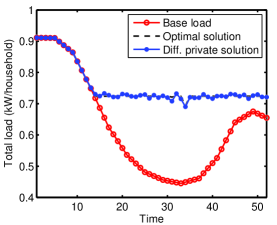
Figure 1: A typical output of the differentially private distributed EV charging algorithm (Algorithm 2) with $\epsilon=0.1$ compared to the optimal solution of problem (2). The other parameters used in the simulation are: $K=6$ and $c=10$.

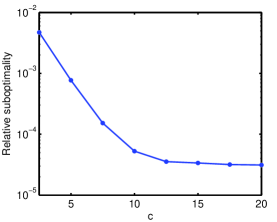
Figure 2: Relative suboptimality of the differentially private distributed EV charging algorithm (Algorithm 2) as a function of the step size constant $c$. The other parameters used in the simulations are: $\epsilon=0.1$ and $K=6$.

Fig. 3 shows the relative suboptimality as a function of $K$. It can be seen from Fig. 3 that an optimal choice of $K$ exists, which coincides with the result of Theorem 7.

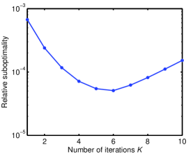
Figure 3: Relative suboptimality of the differentially private distributed EV charging algorithm (Algorithm 2) as a function of the number of iterations $K$. The other parameters used in the simulations are: $\epsilon=0.1$ and $c=10$.

Fig. 4 shows the dependence of the relative suboptimality on $\epsilon$. A separate experiment for investigating the dependence on $n$ is not performed, since changing $n$ is expected to have a similar effect as changing $\epsilon$ according to Corollary 9. As the privacy requirement becomes less stringent (i.e., as $\epsilon$ grows), the suboptimality of Algorithm 2 improves, which coincides qualitatively with the bound given in Corollary 9. One can quantify the relationship between the suboptimality and $\epsilon$ from the slope of the curve in Fig. 4; if the slope is $s$, then the relationship between the suboptimality and $\epsilon$ is given by $\mathcal{O}(\epsilon^{s})$. By performing linear regression on the curve in Fig. 4, we can obtain the slope as $s\approx-0.698$, which is in contrast to $-0.25$ given by Corollary 9. This implies that the suboptimality of Algorithm 2 decreases faster than the rate given by Corollary 9 as $\epsilon$ increases. In other words, the bound given by Corollary 9 is likely to be loose; this is possibly due to the fact that the result on the suboptimality of stochastic gradient descent (Proposition 14) does not consider additional properties of the objective function such as strong convexity.

Figure 4: Relative suboptimality of Algorithm 2 as a function of $\epsilon$. Larger $\epsilon$ implies that less privacy is preserved. The slope is approximately $-0.698$ (compared to the theoretical bound $-0.25$ as given by Corollary 9). All simulations use $c=10$. The number of iterations $K$ is optimized for every choice of $\epsilon$.

VIII Conclusions

This paper develops an $\epsilon$-differentially private algorithm for distributed constrained optimization. The algorithm preserves privacy in the specifications of user constraints by adding noise to the public coordination signal (i.e., gradients). By using the sequential adaptive composition theorem, we show that the noise magnitude is determined by the sensitivity of the projection operation $\Pi_{\mathcal{C}}$, where $\mathcal{C}$ is the parameterized set describing the user constraints. By viewing the projection operation as a least-squares problem, we are able to compute the sensitivity of $\Pi_{\mathcal{C}}$ through a solution sensitivity analysis of optimization problems. We demonstrate how this sensitivity can be computed in the case of EV charging.

We also analyze the trade-off between privacy and performance of the algorithm through results on suboptimality analysis of the stochastic gradient descent method. Specifically, in the case of EV charging, the expected suboptimality of the $\epsilon$-differentially private optimization algorithm with $n$ participating users is upper bounded by $\mathcal{O}((n\epsilon)^{-1/4})$. For achieving the best suboptimality, both the suboptimality analysis and numerical simulations show that there exists an optimal choice for the number iterations: too few iterations affects the convergence behavior, whereas too many iterations leads to too much noise in the gradients. Simulations have indicated that the bound $\mathcal{O}((n\epsilon)^{-1/4})$ is likely not tight. One future direction is to derive a tighter bound for similar distributed optimization problems using information-theoretic approaches (e.g., [6, 21]).

Appendix A Proof of Lemma 13

Consider any adjacent $D$ and $D^{\prime}$ such that $\mathcal{C}_{j}=\mathcal{C}_{j}^{\prime}$ for all $j\neq i$. We will first show that when the outputs of $\hat{p}^{(1)},\hat{p}^{(2)},\dots,\hat{p}^{(k-1)}$ are given, we have

$$\left\|r_{i}^{(k)}(D^{\prime})-r_{i}^{(k)}(D)\right\| \leq(k-1)\Delta,$$

$$\left\|r_{j}^{(k)}(D^{\prime})-r_{j}^{(k)}(D)\right\| =0,\quad\forall j\neq i.$$

We will prove the above result by induction. For $k=1$, we have $\left\|r_{i}^{(1)}(D^{\prime})-r_{i}^{(1)}(D)\right\|=0$ for all $i\in[n]$.

Consider the case when $k>1$. For notational convenience, we define for $i\in[n]$,

$$v_{i}^{(k-1)}(D):=r_{i}^{(k-1)}(D)-\alpha_{k-1}\hat{p}^{(k-1)}.$$ (26)

In (26), we have used the fact that the output of $\hat{p}^{(k-1)}$ is given so that the dependence of $\hat{p}^{(k-1)}$ on $D$ is dropped according to the adaptive sequential composition theorem (Proposition 12). Then, for all $j\neq i$, we have

$$\left\|r_{j}^{(k)}(D^{\prime})-r_{j}^{(k)}(D)\right\|$$

$$\qquad=\left\|\Pi_{\mathcal{C}_{j}^{\prime}}(v_{j}^{(k-1)}(D^{\prime}))-\Pi_{\mathcal{C}_{j}}(v_{j}^{(k-1)}(D))\right\|$$

$$\qquad=\left\|\Pi_{\mathcal{C}_{j}}(v_{j}^{(k-1)}(D^{\prime}))-\Pi_{\mathcal{C}_{j}}(v_{j}^{(k-1)}(D))\right\|$$

$$\qquad\leq\left\|v_{j}^{(k-1)}(D^{\prime})-v_{j}^{(k-1)}(D)\right\|$$

$$\qquad=\left\|r_{j}^{(k-1)}(D^{\prime})-r_{j}^{(k-1)}(D)\right\|=0$$

and

$$\left\|r_{i}^{(k)}(D^{\prime})-r_{i}^{(k)}(D)\right\|$$

$$\qquad=\left\|\Pi_{\mathcal{C}_{i}^{\prime}}(v_{i}^{(k-1)}(D^{\prime}))-\Pi_{\mathcal{C}_{i}}(v_{i}^{k-1)}(D))\right\|$$

$$\qquad\leq\left\|\Pi_{\mathcal{C}_{i}^{\prime}}(v_{i}^{(k-1)}(D^{\prime}))-\Pi_{\mathcal{C}_{i}}(v_{i}^{k-1)}(D^{\prime}))\right\|$$

$$\qquad\qquad+\left\|\Pi_{\mathcal{C}_{i}}(v_{i}^{(k-1)}(D^{\prime}))-\Pi_{\mathcal{C}_{i}}(v_{i}^{k-1)}(D))\right\|$$

$$\qquad\leq\Delta+\left\|v_{i}^{(k-1)}(D^{\prime})-v_{i}^{(k-1)}(D)\right\|$$

$$\qquad=\Delta+\left\|r_{i}^{(k-1)}(D^{\prime})-r_{i}^{(k-1)}(D)\right\|\leq(k-1)\Delta,$$

where we have used the induction hypothesis

$$\left\|r_{i}^{(k-1)}(D^{\prime})-r_{i}^{(k-1)}(D)\right\| \leq(k-2)\Delta,$$

$$\left\|r_{j}^{(k-1)}(D^{\prime})-r_{j}^{(k-1)}(D)\right\| =0,\quad\forall j\neq i.$$

Then, the $\ell_{2}$-sensitivity of $p^{(k)}$ can be computed as follows:

$$\left\|p^{(k)}(D^{\prime})-p^{(k)}(D)\right\|\\ \leq L\left\|\sum_{i=1}^{n}\left[r_{i}^{(k)}(D^{\prime})-r_{i}^{(k)}(D)\right]\right\|\leq L(k-1)\Delta.$$

Since the above results hold for all $i$ such that $D$ and $D^{\prime}$ satisfy $\mathcal{C}_{j}=\mathcal{C}_{j}^{\prime}$ for all $j\neq i$, we have

$$\Delta^{(k)} :=\max_{D,D^{\prime}\colon\mathrm{Adj}(D,D^{\prime})}\left\|p^{(k)}(D^{\prime})-p^{(k)}(D)\right\|$$

$$=\max_{i\in[n]}\max\Bigl{\{}\left\|p^{(k)}(D^{\prime})-p^{(k)}(D)\right\|\colon D,D^{\prime}\text{ satisfy}$$

$$\qquad\mathcal{C}_{j}=\mathcal{C}_{j}^{\prime}\text{ for all }j\neq i\Bigr{\}}$$

$$=L(k-1)\Delta.$$

Appendix B Proofs on the local solution sensitivities

B-A Proof of Lemma 18

The Lagrangian of problem (16) can be written as

$$L(x,\lambda,\mu,\nu)=\frac{1}{2}\left\|x-x_{0}\right\|^{2}-\lambda^{T}x+\mu^{T}(x-a)+\nu(b-\mathbf{1}^{T}x).$$ (27)

Denote by $\lambda^{*}$, $\mu^{*}$, and $\nu^{*}$ the corresponding optimal Lagrange multipliers. It can be verified that all conditions in Proposition 17 hold. Apply Proposition 17 to obtain

$$\partial_{b}x^{*}-\partial_{b}\lambda^{*}+\partial_{b}\mu^{*}-\partial_{b}\nu^{*}\cdot\mathbf{1} =0$$ (28)

$$\mathbf{1}^{T}\partial_{b}x^{*} =1$$ (29)

$$\lambda_{i}^{*}\cdot\partial_{b}x_{i}^{*}+x_{i}^{*}\cdot\partial_{b}\lambda_{i}^{*} =0,\quad i\in[T]$$ (30)

$$\mu_{i}^{*}\cdot\partial_{b}x_{i}^{*}+(x_{i}^{*}-a_{i})\cdot\partial_{b}\mu_{i}^{*} =0,\quad i\in[T].$$ (31)

Strict complementary slackness implies that either (1) $x_{i}^{*}=0$ and $\lambda_{i}^{*}>0$, so that $\partial_{b}x_{i}^{*}=0$ according to (30); or (2) $x_{i}^{*}\neq 0$ and $\lambda_{i}^{*}=0$, so that $\partial_{b}\lambda_{i}^{*}=0$ also according to (30). In other words, under strict complementary slackness, condition (30) is equivalent to

$$\partial_{b}\lambda_{i}^{*}\cdot\partial_{b}x_{i}^{*}=0.$$ (32)

Similarly, we can rewrite condition (31) as

$$\partial_{b}\mu_{i}^{*}\cdot\partial_{b}x_{i}^{*}=0.$$ (33)

Conditions (32) and (33) imply that one and only one of the following is true for any $i\in[T]$: (1) $\partial_{b}x_{i}^{*}=0$; (2) $\partial_{b}\lambda_{i}^{*}=0$ and $\partial_{b}\mu_{i}^{*}=0$. Define $\mathcal{I}:=\{i\colon\partial_{b}x_{i}^{*}\neq 0\}$, and we have

$$\sum_{i\in\mathcal{I}}\partial_{b}x_{i}^{*}=1$$ (34)

from (29). Note that (28) implies that for all $i,j\in[T]$,

$$\partial_{b}x_{i}^{*}-\partial_{b}\lambda_{i}^{*}+\partial_{b}\mu_{i}^{*}=\partial_{b}x_{j}^{*}-\partial_{b}\lambda_{j}^{*}+\partial_{b}\mu_{j}^{*}.$$

Since $\partial_{b}\lambda_{i}^{*}=0$ and $\partial_{b}\mu_{i}^{*}=0$ for all $i\in\mathcal{I}$, we have $\partial_{b}x_{i}^{*}=\partial_{b}x_{j}^{*}$ for all $i,j\in\mathcal{I}$ and hence $\partial_{b}x_{i}^{*}=1/|\mathcal{I}|$ for all $i\in\mathcal{I}$ according to (34). On the other hand, from the definition of $\mathcal{I}$, we have $\partial_{b}x_{i}^{*}=0$ for all $i\notin\mathcal{I}$. In summary, we have $\partial_{b}x^{*}\succeq 0$, which complete the proof.

B-B Proof of Lemma 19

The optimality conditions for problem (16) imply that

$$x^{*}-\lambda^{*}+\mu^{*}-\nu^{*}\mathbf{1} =x_{0}$$ (35)

$$\mathbf{1}^{T}x^{*} =b$$ (36)

$$\lambda_{i}^{*}x_{i}^{*} =0,\quad i\in[T]$$ (37)

$$\mu_{i}^{*}(x_{i}^{*}-a_{i}) =0,\quad i\in[T].$$ (38)

Suppose strict complementary slackness fails for a certain value of $b$. Denote the set of indices of the constraints that violate strict complementary slackness by $\mathcal{I}_{\lambda}:=\{i\colon\lambda_{i}^{*}=0,\>x_{i}^{*}=0\}$ and $\mathcal{I}_{\mu}:=\{i\colon\mu_{i}^{*}=0,\>x_{i}^{*}=a_{i}\}$. If both $\mathcal{I}_{\lambda}$ and $\mathcal{I}_{\mu}$ are empty, then strict complementary slackness holds for all constraints.

Proof:

When $\mathcal{I}_{\lambda}$ is non-empty, we know from (38) that $\mu_{i}^{*}=0$ for all $i\in\mathcal{I}_{\lambda}$. For any $i\in\mathcal{I}_{\lambda}$, substitute $x_{i}^{*}=0$, $\lambda_{i}^{*}=0$, and $\mu_{i}^{*}=0$ into (35) to obtain $\nu^{*}=x_{0,i}$. For any other $j\notin\mathcal{I}_{\lambda}$, one of the following three cases must hold: (1) $x_{j}^{*}=0$; (2) $x_{j}^{*}=a_{j}$; (3) $0<x_{j}^{*}<a_{j}$. Consider a partition $(\mathcal{I}_{1},\mathcal{I}_{2},\mathcal{I}_{3})$ of the set $[n]\backslash\mathcal{I}_{\lambda}$ as follows:

$$\mathcal{I}_{1}:=\{j\colon x_{j}^{*}=0\},\qquad\mathcal{I}_{2}:=\{j\colon x_{j}^{*}=a_{j}\},$$

$$\mathcal{I}_{3}:=\{j\colon 0<x_{j}^{*}<a_{j}\}.$$

For any $j\in\mathcal{I}_{3}$, we have $\lambda_{j}^{*}=\mu_{j}^{*}=0$ from (30) and (31), so that we have $x_{j}^{*}=\nu^{*}+x_{0,j}$ according to (28). Then, we can write using (36)

$$b =\mathbf{1}^{T}x^{*}$$

$$=\sum_{i\in\mathcal{I_{\lambda}}}x_{i}^{*}+\sum_{j\in\mathcal{I}_{1}}x{}_{j}^{*}+\sum_{j\in\mathcal{I}_{2}}x_{j}^{*}+\sum_{j\in\mathcal{I}_{3}}x_{j}^{*}$$

$$=|\mathcal{I}_{\lambda}|\nu^{*}+0+\sum_{j\in\mathcal{I}_{2}}a_{j}+\sum_{j\in\mathcal{I}_{3}}(\nu^{*}+x_{0,j}).$$ (39)

Since both $a$ and $x_{0}$ are fixed, we know that the choice of $\nu^{*}=x_{0,i}$ (for any $i\in\mathcal{I}_{\lambda}$) is finite. By enumerating all finitely many partitions $(\mathcal{I}_{\lambda},\mathcal{I}_{1},\mathcal{I}_{2},\mathcal{I}_{3})$ of $[T]$, we know that $b$ can only take finitely many values according to (39). The proof is similar for the case when $\mathcal{I}_{\mu}$ is nonempty by making use of (37). When both $\mathcal{I}_{\lambda}$ and $\mathcal{I}_{\mu}$ are nonempty, the possible values of $b$ are given by the intersection of those when only one of $\mathcal{I}_{\lambda}$ and $\mathcal{I}_{\mu}$ is empty; hence the number of possible values is also finite. ∎

B-C Proof of Lemma 21

Similar to the proof of Lemma 18, we apply Proposition 17 using the Lagrangian as given by (27). We can show that the following holds for all $i\in[T]$:

$$\partial_{a_{i}}x_{i}^{*}-\partial_{a_{i}}\lambda_{i}^{*}+\partial_{a_{i}}\mu_{i}^{*}-\partial_{a_{i}}\nu^{*} =0$$ (40)

$$\partial_{a_{j}}x_{i}^{*}-\partial_{a_{j}}\nu^{*} =0,\quad\forall j\neq i$$ (41)

$$\lambda_{i}^{*}\partial_{a_{j}}x_{i}^{*}+x_{i}^{*}\partial_{a_{j}}\lambda_{i}^{*} =0,\quad\forall j\in[T]$$ (42)

$$\mu_{i}^{*}\partial_{a_{j}}x_{i}^{*}+(x_{i}^{*}-a_{i})\partial_{a_{j}}\mu_{i}^{*}-\mu_{i}^{*} =0$$ (43)

$$\mu_{i}^{*}\partial_{a_{j}}x_{i}^{*}+(x_{i}^{*}-a_{i})\partial_{a_{j}}\mu_{i}^{*} =0,\quad\forall j\neq i$$ (44)

$$\sum_{j=1}^{n}\partial_{a_{i}}x_{j}^{*} =0.$$ (45)

From (40) and (41), we know that the following holds for all $i$:

$$\partial_{a_{i}}\nu^{*}=\partial_{a_{i}}x_{i}^{*}-\partial_{a_{i}}\lambda_{i}^{*}+\partial_{a_{i}}\mu_{i}^{*}=\partial_{a_{i}}x_{j}^{*},\quad\forall j\neq i.$$ (46)

The first equality in (46) implies that there exists a constant $C_{i}$ such that $\partial_{a_{i}}x_{j}^{*}=C_{i}$ for all $j\neq i$. Then, we can rewrite (45) as

$$\partial_{a_{i}}x_{i}^{*}+(T-1)C_{i}=0,\quad\forall i\in[T],$$ (47)

which implies that

$$\left\|\partial_{a_{i}}x^{*}\right\|_{1}=\sum_{j=1}^{T}|\partial_{a_{i}}x_{j}^{*}|=|\partial_{a_{i}}x_{i}^{*}|+\sum_{j\neq i}|\partial_{a_{i}}x_{j}^{*}|$$

$$\qquad=2(T-1)|C_{i}|.$$ (48)

Suppose strict complementary slackness holds. Then, for any $i\in[T]$, only one of the three following cases holds:

1. $x_{i}^{*}=0$, $\lambda_{i}^{*}>0$, $\mu_{i}^{*}=0$;

2. $x_{i}^{*}=a_{i}$, $\lambda_{i}^{*}=0$, $\mu_{i}^{*}>0$;

3. $0<x_{i}^{*}<a_{i}$, $\lambda_{i}^{*}=0$, $\mu_{i}^{*}=0$.

In the next, we will derive the expression of $\left\|\partial_{a_{i}}x^{*}\right\|_{1}$ for the three cases separately:

1. $x_{i}^{*}=0$, $\lambda_{i}^{*}>0$, $\mu_{i}^{*}=0$:

   Using (42), we obtain $\partial_{a_{j}}x_{i}^{*}=0$ for all $j\in[T]$; in particular, this implies $\partial_{a_{i}}x_{i}^{*}=0$. Substituting $\partial_{a_{i}}x_{i}^{*}=0$ into (47), we obtain $C_{i}=0$, so that $\left\|\partial_{a_{i}}x^{*}\right\|_{1}=0$ according to (48).

2. $x_{i}^{*}=a_{i}$, $\lambda_{i}^{*}=0$, $\mu_{i}^{*}>0$:

   Using (43), we obtain $\partial_{a_{i}}x_{i}^{*}=1$; substitute this into (47) to obtain $C_{i}=-\frac{1}{T-1}$, so that we have $\left\|\partial_{a_{i}}x^{*}\right\|_{1}=2$ according to (48).

3. $0<x_{i}^{*}<a_{i}$, $\lambda_{i}^{*}=0$, $\mu_{i}^{*}=0$:

   Using (42)–(44), we obtain $\partial_{a_{j}}\lambda_{i}^{*}=\partial_{a_{j}}\mu_{i}^{*}=0$ for all $j\in[T]$; in particular, this implies $\partial_{a_{i}}\lambda_{i}^{*}=\partial_{a_{i}}\mu_{i}^{*}=0$. Then, using (46), we have $\partial_{a_{i}}x_{i}^{*}=C_{i}$; substitute this into (47) to obtain $C_{i}=0$, so that $\left\|\partial_{a_{i}}x^{*}\right\|_{1}=0$ according to (48).

For case 2 in the above, the fact that $\partial_{a_{i}}x_{j}^{*}=C_{i}=-\frac{1}{T-1}\neq 0$ for all $j\neq i$ also implies that $x_{j}^{*}\neq a_{j}$ for all $j\neq i$. Otherwise, the fact $x_{j}^{*}=a_{j}$ would imply $\mu_{j}^{*}>0$ as a result of strict complementary slackness. According to (44), we have

$$\mu_{j}^{*}\partial_{a_{i}}x_{j}^{*}+(x_{j}^{*}-a_{j})\partial_{a_{i}}\mu_{j}^{*}=0,\quad\forall i\neq j,$$

so that $\mu_{j}^{*}>0$ would imply $\partial_{a_{i}}x_{j}^{*}=0$, which causes a contradiction. To summarize, there exists at most one $i\in[T]$ such that $\left\|\partial_{a_{i}}x^{*}\right\|_{1}=2$ (i.e., case 2 holds), whereas for other $j\neq i$ we have $\left\|\partial_{a_{j}}x^{*}\right\|_{1}=0$ (i.e., either case 1 or 3 holds). This implies that $\sum_{j=1}^{T}\left\|\partial_{a_{j}}x^{*}\right\|_{1}\leq 2$, which completes the proof.

B-D Proof of Lemma 22

Define $\mathcal{I}_{\mu}=\{i\colon\mu_{i}^{*}=0,\>x_{i}^{*}=a_{i}\}$. If $\mathcal{I}_{\mu}$ is empty, then strict complementary slackness for the constraint $x\preceq a$ holds. For any $i\in\mathcal{I}_{\mu}$, we have $\nu^{*}=a_{i}-x_{0,i}$ and $\lambda_{i}^{*}=0$ according to (35) and (37). For any other $j\notin\mathcal{I}_{\mu}$, one of the following three cases must hold: (1) $x_{j}^{*}=0$; (2) $x_{j}^{*}=a_{j}$; (3) $0<x_{j}^{*}<a_{j}$. The last case implies that $\lambda_{j}^{*}=\mu_{j}^{*}=0$, so that we have $x_{j}^{*}=a_{i}-x_{0,i}+x_{0,j}$, where $i\in\mathcal{I}_{\lambda}$. Since both $b$ and $x_{0}$ are fixed, and only one $a_{i}$ among all $i\in[T]$ is allowed to change due to the constraint imposed by the integration path $L$, we can use a similar argument as the one in the proof of Lemma 19 to conclude that there are finitely many values of $a$ along $L$ such that the constraint $b=\mathbf{1}^{T}x^{*}$ is satisfied.

References

• [1] C. Berge. Topological Spaces: Including a Treatment of Multi-Valued Functions, Vector Spaces and Convexity. Courier Dover Publications, 1963.
• [2] E. S. Canepa and C. G. Claudel. A framework for privacy and security analysis of probe-based traffic information systems. In ACM International Conference on High Confidence Networked Systems, pages 25–32, 2013.
• [3] K. Clement-Nyns, E. Haesen, and J. Driesen. The impact of charging plug-in hybrid electric vehicles on a residential distribution grid. IEEE Transactions on Power Systems, 25(1):371–380, 2010.
• [4] G. B. Dantzig, J. Folkman, and N. Shapiro. On the continuity of the minimum set of a continuous function. Journal of Mathematical Analysis and Applications, 17(3):519–548, 1967.
• [5] S. Deilami, A. S. Masoum, P. S. Moses, and M. A. S. Masoum. Real-time coordination of plug-in electric vehicle charging in smart grids to minimize power losses and improve voltage profile. IEEE Transactions on Smart Grid, 2(3):456–467, 2011.
• [6] J. C. Duchi, M. I. Jordan, and M. J. Wainwright. Local privacy and statistical minimax rates. In IEEE Annual Symposium on Foundations of Computer Science, pages 429–438, 2013.
• [7] C. Dwork. Differential privacy: A survey of results. In Theory and Applications of Models of Computation, pages 1–19. Springer, 2008.
• [8] C. Dwork, F. McSherry, K. Nissim, and A. Smith. Calibrating noise to sensitivity in private data analysis. In Theory of Cryptography, pages 265–284. Springer, 2006.
• [9] C. Dwork and A. Roth. The algorithmic foundations of differential privacy. Theoretical Computer Science, 9(3-4):211–407, 2013.
• [10] A. V. Fiacco. Sensitivity analysis for nonlinear programming using penalty methods. Mathematical programming, 10(1):287–311, 1976.
• [11] L. Gan, U. Topcu, and S. H. Low. Optimal decentralized protocol for electric vehicle charging. IEEE Transactions on Power Systems, 28(2):940–951, 2013.
• [12] S. W. Hadley and A. A. Tsvetkova. Potential impacts of plug-in hybrid electric vehicles on regional power generation. The Electricity Journal, 22(10):56–68, 2009.
• [13] J. Hsu, Z. Huang, A. Roth, T. Roughgarden, and Z. S. Wu. Private matchings and allocations. arXiv preprint arXiv:1311.2828, 2013.
• [14] J. Hsu, A. Roth, T. Roughgarden, and J. Ullman. Privately solving linear programs. Automata, Languages, and Programming, 8572:612–624, 2014.
• [15] Z. Huang, S. Mitra, and N. Vaidya. Differentially private distributed optimization. arXiv preprint arXiv:1401.2596, 2014.
• [16] A. Ipakchi and F. Albuyeh. Grid of the future. IEEE Power and Energy Magazine, 7(2):52–62, 2009.
• [17] M. Kearns, M. Pai, A. Roth, and J. Ullman. Mechanism design in large games: Incentives and privacy. In Conference on Innovations in Theoretical Computer Science, pages 403–410, 2014.
• [18] J. Le Ny and G. J. Pappas. Differentially private filtering. IEEE Transactions on Automatic Control, 59(2):341–354, 2014.
• [19] Z. Ma, D. S. Callaway, and I. A. Hiskens. Decentralized charging control of large populations of plug-in electric vehicles. IEEE Transactions on Control Systems Technology, 21(1):67–78, 2013.
• [20] A. Narayanan and V. Shmatikov. How to break anonymity of the Netflix prize data set. The University of Texas at Austin, 2007.
• [21] M. Raginsky and A. Rakhlin. Information-based complexity, feedback and dynamics in convex programming. IEEE Transactions on Information Theory, 57(10):7036–7056, 2011.
• [22] H. Robbins and S. Monro. A stochastic approximation method. The Annals of Mathematical Statistics, 22(3):400–407, 1951.
• [23] R. M. Rogers and A. Roth. Asymptotically truthful equilibrium selection in large congestion games. In ACM Conference on Economics and Computation, pages 771–782, 2014.
• [24] L. Sankar, S. R. Rajagopalan, S. Mohajer, and H. V. Poor. Smart meter privacy: A theoretical framework. IEEE Transactions on Smart Grid, 4(2):837–846, 2013.
• [25] O. Shamir and T. Zhang. Stochastic gradient descent for non-smooth optimization: Convergence results and optimal averaging schemes. In International Conference on Machine Learning, pages 71–79, 2013.
• [26] E. Sortomme, M. M. Hindi, S. D. J. MacPherson, and S. S. Venkata. Coordinated charging of plug-in hybrid electric vehicles to minimize distribution system losses. IEEE Transactions on Smart Grid, 2(1):198–205, 2011.
• [27] J. Taylor, A. Maitra, M. Alexander, D. Brooks, and M. Duvall. Evaluations of plug-in electric vehicle distribution system impacts. In IEEE Power and Energy Society General Meeting, pages 1–6, 2010.
• [28] J. A. Tropp, I. S. Dhillon, R. W. Heath, and T. Strohmer. Designing structured tight frames via an alternating projection method. IEEE Transactions on Information Theory, 51(1):188–209, 2005.
• [29] P. Venkitasubramaniam. Privacy in stochastic control: A markov decision process perspective. In Annual Allerton Conference on Communication, Control, and Computing, pages 381–388, 2013.