Anisotropic Agglomerative Adaptive Mean-Shift

Abstract

Mean Shift today, is widely used for mode detection and clustering. The technique though, is challenged in practice due to assumptions of isotropicity and homoscedasticity. We present an adaptive Mean Shift methodology that allows for full anisotropic clustering, through unsupervised local bandwidth selection. The bandwidth matrices evolve naturally, adapting locally through agglomeration, and in turn guiding further agglomeration. The online methodology is practical and effecive for low-dimensional feature spaces, preserving better detail and clustering salience. Additionally, conventional Mean Shift either critically depends on a per instance choice of bandwidth, or relies on offline methods which are inflexible and/or again data instance specific. The presented approach, due to its adaptive design, also alleviates this issue - with a default form performing generally well. The methodology though, allows for effective tuning of results.

1 Introduction

‘Mean Shift’ ([15, 7], MS) is a powerful nonparametric technique for unsupervised pattern clustering and mode seeking. References [11, 3] established it’s utility in low-level perception tasks such as feature clustering, filtering and in tracking. It has been in popular use since, as a very useful tool for pattern clustering of sensor data ([28, 14] for example). It has also found niche as a preprocessor (a priori segmentation, smoothing) before higher level image & video analysis tasks such as scene parsing, object recognition, detection ([22, 35, 20]). Image segmentation approaches such as Markov Random Fields, Spectral clustering, Hierarchical clustering use it as an a priori segmenter with improved results ([22, 26, 21, 31, 30]).

Mean Shift methodologies though, employ some assumptions and have some limitations, which may not be desirable. Its popular standard form, [11], utilizes fixed, scalar bandwidth assuming homoscedasticity and isotropicity. Being homoscedastic, it also requires proper bandwidth choice on a per instance basis. The adaptive Mean Shift variants, [12, 16], ascertain variable bandwidths, but they still assume isotropicity. They also make use of heuristics which are not flexible, and lack clustering control. Offline bandwidth selection methods for Mean Shift ([6, 17, 10]), typically estimate a single, global bandwidth, and/or are data specific/non-automatic. As indicated in Fig.1 - isotropic/scalar bandwidths tend to smooth anisotropic patterns and affect partition boundaries, while global/homoscedastic bandwidths are inappropriate when clusters (or modes) at different scales need to be identified.

We present a Mean Shift methodology which is anisotropic and locally adaptive. It is able to leverage guided agglomeration for unsupervised bandwidth selection (Fig.1, 5). This results in robust mode detection, with increased partition saliency. Also as a consequence, a low valued parameter set performs nicely over a wider range of data instances (Sec. 2.1).

Clusters arise on the fly in the proposed approach, as a consequence of agglomeration of extant clusters. Local bandwidths (Secs. 1.1, 2) which evolve anisotropically every iteration, are associated with each cluster; by design, all members of a cluster converge to the same local mode. By evolving as function of a cluster’s aggregated trajectory points, these bandwidths are able to adapt to the underlying mode structure (shape, scale, orientation) - and in turn, guide future cluster trajectory and agglomeration. The supplementary also presents a useful result - a convergence proof when full bandwidths vary between Mean Shift iterations, as is the case here. We refer to our approach as online because it’s an on the fly unsupervised procedure; with simple bookkeeping doing away with re-calculations.

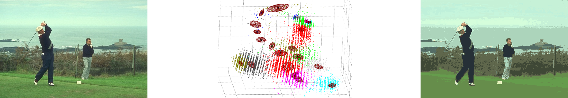
(a) 3D Clustering result ($23$ clusters) over image data (left, L*a*b* space) by the proposed approach. 1-sigma final trajectory bandwidths have been overlaid over the converged modes. The segment image is shown on right.

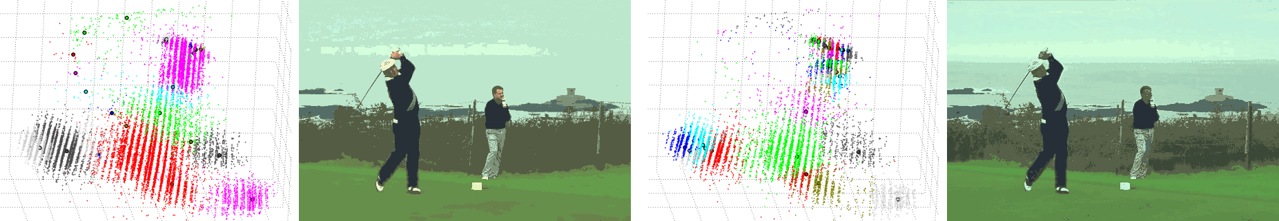
(b) Comparitive results with standard MS (left) and variable-bandwidth isotropic MS ([16], right), at similar clustering levels, $25$ & $27$ respectively, are shown. Final mode locations have been indicated over the cluster plots. MS with correctly chosen bandwidth detected more coherent modes than [16], but looses partition saliency (bushes, water, sky in background). [16] better adapts to scales but oversegments at places, and smooths over others (face). Both smoothed over details, failed to detect some modes at lower scales (trouser edges, maroon on shirt & shoes). In general, conventional MS had a typical tendency to over-segment heavily or compromise partition boundaries.

Figure 1: Exemplar illustrative result of our approach, AAAMS (a), is shown along with conventional MS results (b), at comparable clustering levels. As is indicated by the plots and segment images, AAAMS effectively adapts to local scale and preserves anisotropic details, affecting more salient partitions.

1.1 Motivation and Background

We utilize the exposition style of [5]. Let $\left\{x_{i}\right\}_{i=1}^{n}\subset R^{d}$, be a set of d-dimensional data points with their sample point kernel density estimate (KDE) being $p(x)=\sum_{i=1}^{n}p(x_{i})p(x|x_{i})=\sum_{i=1}^{n}p_{i}\frac{1}{c_{i}}K(\|x-x_{i}\|_{\Sigma_{i}})$. Stationary points of the KDE can be estimated by evaluating the density gradient and setting it to zero. This gives rise to the Mean-Shift fixed point iteration :

$$x^{\text{$\tau$+1}}=f(x^{\tau})$$ (1a)

$$f(x^{\tau})=\bigg{(}\sum_{i=1}^{n}p_{i}\frac{1}{c_{i}}K^{{}^{\prime}}(\|x^{\tau}-x_{i}\|_{\Sigma_{i}})\Sigma_{i}^{-1}\bigg{)}^{-1}\times\bigg{(}\sum_{i=1}^{n}p_{i}\frac{1}{c_{i}}K^{{}^{\prime}}(\|x^{\tau}-x_{i}\|_{\Sigma_{i}})\Sigma_{i}^{-1}x_{i}\bigg{)}$$ (1b)

$K(t),\,t\geq 0$, is a d-variate kernel with compact support satisfying some regularity constraints, mild in practice ([11, 5] for details). $\|x-x_{i}\|_{\Sigma_{i}}\equiv((x-x_{i})^{T}\Sigma_{i}^{-1}(x-x_{i}))^{\nicefrac{{1}}{{2}}}$, is the Mahanalobis metric. The point prior $p_{i}\equiv p(x_{i})$ is usually taken as $\nicefrac{{1}}{{n}}$. $c_{i}$ is a normalizing constant depending only on the covariance matrix, $\Sigma_{i}$ (kernel bandwidth), associated with each data point. The bandwidth, $\Sigma_{i}$, is roughly an inverse measure of local curvature around $x_{i}$. It linearly captures the scale and correlations of the underlying data. $\tau$ indicates the iteration count. In practice, since $K(t)$ is taken with truncated support, the summations are only over $n^{\prime}$ neighbors of $x^{\tau}$, with $n^{\prime}\ll n$. The vector $m(x^{\tau})=f(x^{\tau})-x^{\tau}$, is referred to as the Mean Shift. It’s a bandwidth scaled version of $\nabla p(x)$, is free from a step size parameter, is large in regions with low $p(x)$ and small near the modes. Starting at a data point, $x_{i}^{\tau=0}\equiv x_{i}$, the fixed point update is run multiple times till convergence. The resulting points, $x_{i}^{\tau\geq 1}$ is referred to as the trajectory of $x_{i}$, tracing a path to the local mode. The technique thus, is able to locate modes and partition feature space, without a priori knowledge of partition count or structure.

The above hinges on selecting reasonable bandwidth matrices $\Sigma_{i}$. Good bandwidths capture the underlying local distribution effectively. In our approach, data points (pertaining to a cluster) converging to a common local mode share a common bandwidth - one which reflects this mode’s structure, and to an extent, its basin of attraction ([11]). We refer to it as the local bandwidth ([10] utilizes local bandwidths in a related sense).

In online unsupervised usage, almost all Mean Shift variants for clustering, for example [11, 30, 37, 27], work under the restrictive assumptions of homoscedasticity and isotropicity ($\Sigma_{i}=\sigma^{2}I$, standard fixed bandwidth Mean Shift). The scale parameter $\sigma$ has to be set carefully based on the dataset instance. [36] utilizes set covering based iterative agglomeration for improved efficiency. Coverage is ensured through overlaps of small fixed homoscedastic bandwidths. Some applications only assume isotropicity ($\Sigma_{i}=\sigma_{i}^{2}I$, adaptive / variable-bandwidth Mean Shift). $\sigma_{i}$ is estimated using a variation of the following two heuristics ([12, 16]) - 1) $k^{th}$ nearest neighbor, $x_{i}^{k}$, distance heuristic $\rightarrow$ $\sigma_{i}\propto\|x_{i}-x_{i}^{k}\|$, or 2) Abramson’s heuristic $\rightarrow$ $\sigma_{i}\propto\sigma_{o}(\pi(x_{i}))^{\nicefrac{{-1}}{{2}}}$, where $\pi(x)$ is the pilot density estimate obtained by first running mean shift with analysis bandwidth, $\sigma_{o}$. They have found more use in smoothing type applications as reported in [25, 19]. Variants have also been used in tracking scenarios, where the bandwidths are adapted in a task specific fashion (see [18, 9], for example). [23, 33] adapt isotropic bandwidths to object scales, to unimodally track, search for them. The topological, blurring, evolving variants for clustering (like [27, 30, 37, 4, 29]) use isotropic bandwidths. They are primarily aimed at increased efficiency, with results on par with standard mean shift. [32] presents improvements over the somewhat related Mediod Shift. They propose usage of their algorithm as initialization for Mean Shift, for increased efficiency.

In offline settings, [10] presents a supervised methodology. Training data is processed with analysis bandwidths to select local bandwidths based on neighboring partition stability. The estimated bandwidths are then used to partition similarly distributed test image data. Only recently were automatic full bandwidth selectors for density gradient estimation proposed in [17, 6], for offline settings. These focus on obtaining good data density gradients (as opposed to clustering) and optimize based on the mean square integrated error (MISE). A single global bandwidth is estimated for the given data, and as the authors themselves note, the involved computations are not straighforward.

A very useful variant is Joint Domain Mean Shift, [11], which is used to create partitions jointly respecting the dataset’s multiple feature domains which are mutually independent; For example, $\left\langle color,space\right\rangle$ in color based segmentation & smoothing, and $\left\langle color,flow\right\rangle$ in motion segmentation. When $x=\left[{x^{r}}^{T}\,{x^{s}}^{T}\right]$ with $\left(x^{r}\,\bot\,x^{s}\right)|x$, and utilizing two separate kernels, $K_{r},\,K_{s}$, we’ll have $p(x)=\sum_{i=1}^{n}p(x_{i})p(x^{r}|x_{i})p(x^{s}|x_{i})$. Eq.1b analogue would then come out to be $f(x^{\tau})=\left(\sum_{i=1}^{n}p_{i}\frac{1}{c_{i}^{{}^{\prime}}}J(\|x^{\tau,r}-{x_{i}}^{r}\|_{\Sigma_{i}^{r}},\|x^{\tau,s}-{x_{i}}^{s}\|_{\Sigma_{i}^{s}})\Sigma_{i}^{-1}\right)^{-1}\times\left(\sum_{i=1}^{n}p_{i}\frac{1}{c_{i}^{{}^{\prime}}}J(\|x^{\tau,r}-{x_{i}}^{r}\|_{\Sigma_{i}^{r}},\|x^{\tau,s}-{x_{i}}^{s}\|_{\Sigma_{i}^{s}})\Sigma_{i}^{-1}x_{i}\right)$, where $c_{i}^{{}^{\prime}}$ is the normalization constant, $J(t_{1},t_{2})\equiv K_{r}^{{}^{\prime}}(t_{1})K_{s}(t_{2})=K_{r}(t_{1})K_{s}^{{}^{\prime}}(t_{1}),\forall t_{1},t_{2}\geq 0$, and $\Sigma_{i}=\left[\begin{array}[]{cc}\Sigma_{i}^{r}&0\\ 0&\Sigma_{i}^{s}\end{array}\right]$. Typically, but not necessarily, $x^{s}$ may lie on a spatial manifold - imposing structure to data which is utilized. Instances in literature use fixed global scale parameters $\sigma^{r}$ and $\sigma^{s}$, which have the aforementioned limitations. As noted in [31] on color segmentation, $\sigma^{r}$ and $\sigma^{s}$ need to be selected carefully. Good choices are not always possible, with segments being too coarse or too fine at times (Figs. 3, 5). Reference [34] utlizes an anisotropic $\Sigma_{i}^{s}$ for visual data segmentations. Every data point’s associated bandwidth, $\Sigma_{i}$, is modulated multiple times in each iteration, until convergence is achieved. Modulation heuristics have been provided, to be deployed as per task. The spatial bandwidth $\Sigma_{i}^{s}$ is parameterized as function of eigenvectors of neighborhood data covariance. $\Sigma_{i}^{r}$ is taken to be an isotropic scalar dependent on $\Sigma_{i}^{s}$.

2 Methodology

A data point, $x_{i}$, is alternatively represented as $x_{i,u}$ - the first index value being its unique identifier as before and the second index indicating its current, exclusive membership to a cluster, $u\in\left\{1,\dots n\right\}$ . A cluster $u$’s constituent data points is denoted by the set , $C_{u}=\{x_{i,u}\mid\exists\,i\in\{1,\dots n\}\}$. By algorithm design, clusters are merged only when they are tending towards the same mode - thus all member points of a cluster, $u$, will eventually converge to a common local mode, say $\mu{}_{u}$. They hence, are also taken to share a common local bandwidth, $\Sigma{}_{u}$. This bandwidth develops every iteration when the cluster $u$’s trajectory points set, $T_{u}$ , gets additional elements. The set of clusters surviving at iteration, $\tau$, would be $U^{\tau}=\left\{u\mid C_{u}\neq\emptyset\right\}$. $\left|U^{\tau}\right|$ would indicate its cardinality. At beginning, at $\tau=0$, each point trivially forms a separate cluster $\rightarrow$ $U^{0}=\{1,\dots n\}$ , $C_{u}=\{x_{i=u,u}\},\,\forall u\in U^{0}$. Given the initialization, each extant cluster $u\in U^{\tau}$ will always contain the initial point, $x_{u,u}$ - which we refer to as its principle member.

At any iteration $\tau$, for each extant cluster $u$, mean shift updates happen for only the principle member, $x_{u,u}$; with the first iteration running over trivial clusters. The resulting trajectory is specified as $x_{u,u}^{\tau\geq 1}$ or simply $u^{\tau}$. A cluster’s trajectory might end when it gets merged or converged. In general, each data point, $x_{i}$, started out as a trivial cluster, and had or still has a trajectory - it’s trajectory set being $\{x_{i}^{\tau=1:end}\}$. ${}^{\prime}end^{\prime}$ being the iteration at which the trajectory ended; else the current iteration. Note that the data point $x_{i}$ itself is not included in this set. For any surviving cluster u, then, the complete set of all agglomerated trajectory points associated with it, would be $T_{u}=\{\cup\,\{x_{i}^{\tau=1:end}\}\mid x_{i}\in C_{u}\}$ - basically a union of all the members’ trajectory sets. $u^{\tau}$ is indicative of the cluster $u$’s location. At convergence, $u^{\tau}$ would be the location of a local mode. $u$’s members would then be comprising of data points pertaining to that mode and its basin (Fig. 1(a)). The data density in the immediate vicinity of $u^{\tau}$’s current position is indicated as $\rho(u^{\tau})$, or simply, $\rho_{u}$. We use operator $\Pi$ to retrieve the cluster identifier of an arbitrary data point; so $\Pi(x_{i,u})=u$. The $n^{\prime}$ data points in $u^{\tau}$’s neighborhood are denoted as $Ne_{x}(u^{\tau})$, and the clusters containing them as $G=\left\{\cup\,\Pi(y)\mid y\in Ne_{x}(u^{\tau})\right\}$.

Algorithm 1 : AAAMS - Anisotropic Agglomerative Adaptive Mean Shift
 

$Function\,:\,AAAMS\left\langle\left\{x_{i}\right\}_{i=1}^{n}\right\rangle\leavevmode\nobreak\ with\leavevmode\nobreak\ x_{i}\in R^{d}$

$Returns\,:\,\left\langle U^{*},\,C^{*},\,\{\mu_{u}\}_{u\in U^{*}},\,\{\Sigma_{u}^{*}\}_{u\in U^{*}}\right\rangle$

$\#\#\leavevmode\nobreak\ Convergence\,Criteria\,\rightarrow\,\left\|m_{u}\right\|\leq\delta$

$U^{o}=\left\{1,\dots n\right\}\leavevmode\nobreak\ ;\leavevmode\nobreak\ C_{u}=\left\{x_{u}\right\},\leavevmode\nobreak\ x_{u}^{o}=x_{u},\leavevmode\nobreak\ \Sigma_{u}=\sigma_{base}^{2}I_{d},\leavevmode\nobreak\ \forall u\in U^{0}$

$\tau=0\leavevmode\nobreak\ ;\leavevmode\nobreak\ \lambda=5\leavevmode\nobreak\ ;\leavevmode\nobreak\ \delta=Convergence\leavevmode\nobreak\ epsilon$

$m_{u}=Large\,\in\,R^{d},\leavevmode\nobreak\ T_{u}=\phi\,,\,\forall u\in U^{0}$

$While\leavevmode\nobreak\ \leavevmode\nobreak\ \exists u\,\in U^{\tau}s.t.\,\left\|m_{u}\right\|>\delta$

$ForEach\leavevmode\nobreak\ \leavevmode\nobreak\ u\,\in\,U^{\tau}\,s.t.\,\left\|m_{u}\right\|>\delta$

$u^{\tau+1}=\begin{cases}\begin{array}[]{c}Eq.\,\ref{eq:ScalarUp}\\ Eq.\,\ref{eq:FullUp}\\ Eq.\,\ref{eq:PartialUp}\end{array}&\begin{array}[]{c}ESS(u)\,<\,\lambda\\ ESS(g)\,\geq\lambda,\,\forall g\in G\\ otherwise\end{array}\end{cases}$

$m_{u}=u^{\tau+1}-u^{\tau}\,;\,T_{u}=T_{u}\cup u^{\tau+1}$

$Get\,Ne_{x}(u^{\tau+1})$

$ForEach\leavevmode\nobreak\ \leavevmode\nobreak\ y\,\in\,Ne_{x}(u^{\tau+1})\leavevmode\nobreak\ or\leavevmode\nobreak\ till\leavevmode\nobreak\ C_{u}\neq\emptyset$

$If\leavevmode\nobreak\ \Pi(y)\,=u\leavevmode\nobreak\ or\leavevmode\nobreak\ C_{\Pi(y)}=\phi\,\,\,Then\,\,\,Continue$

$If\leavevmode\nobreak\ \left\|u^{\tau+1}-y\right\|>\epsilon\,\,\,Then\,\,\,Continue$

$If\leavevmode\nobreak\ !MergeCheck\left\langle u^{\tau+1},y,m_{u},y^{\tau=1}-y,u,\Pi(y)\right\rangle$

$Then\leavevmode\nobreak\ Continue$

$If\leavevmode\nobreak\ \rho_{u}>\rho_{\Pi(y)\,}$

$Then$

$C_{u}=C_{u}\cup C_{\Pi(y)}\,;\,C_{\Pi(y)}=\emptyset$

$T_{u}=T_{u}\cup T_{\Pi(y)}\,;\,T_{\Pi(y)}=\emptyset$

$Else$

$C_{\Pi(y)}=C_{u}\cup C_{\Pi(y)}\,;\,C_{u}=\emptyset$

$T_{\Pi(y)}=T_{u}\cup T_{\Pi(y)}\,;\,T_{u}=\emptyset$

$EndForEach$

$If\leavevmode\nobreak\ C_{u}=\phi\,\,\,\,Then\,\,\,Continue$

$\Sigma_{u}=\begin{cases}\begin{array}[]{c}Eq.\,\ref{eq:band}\\ \Sigma_{u}\end{array}&\begin{array}[]{c}ESS(u)\,\geq\,\lambda\\ otherwise\end{array}\end{cases}$

## $Optionally\leavevmode\nobreak\ Perturb\left\langle u^{\tau+1},\,m_{u}\right\rangle\leavevmode\nobreak\ \leavevmode\nobreak\ if\leavevmode\nobreak\ \left\|m_{u}\right\|\leq\delta$

$EndForEach$

$U^{\tau+1}=\left\{u\mid u\,\in\,U^{\tau},\,C_{u}\neq\emptyset\right\}$

$\tau=\tau+1$

$EndWhile$

$U^{*}=U^{\tau}$ ;  $C^{*}=C_{u}\,,\,\forall u\in U^{\tau}$ ;   $\Sigma_{u}^{*}=\Sigma_{u}\,,\,\forall u\in U^{\tau}$

$EndFunction$

 
For feature spaces that can be decomposed into independent subspaces, the above can be extended to multiple domains. The update equations would then utlize multiple kernels. Basically, for each domain, a $\left\langle\sigma_{base},\,\epsilon\right\rangle$ pair needs to be set.

For example, for joint domain Mean Shift (Sec:1.1), we’ll have $\left\langle\sigma_{base}^{r},\,\epsilon^{r}\right\rangle\,\&\,\left\langle\sigma_{base}^{s},\,\epsilon^{s}\right\rangle$ for the two domains. We’ll have then $\Sigma_{base}=\bigg{[}\begin{array}[]{cc}\sigma_{base}^{r^{2}}I_{r}&0\\ 0&\sigma_{base}^{s^{2}}I_{s}\end{array}\bigg{]}\leavevmode\nobreak\ \&\leavevmode\nobreak\ \Sigma_{u}=\left[\begin{array}[]{cc}\Sigma_{u}^{r}&0\\ 0&\Sigma_{u}^{s}\end{array}\right]$. $\Sigma_{u}^{r}\leavevmode\nobreak\ \&\leavevmode\nobreak\ \Sigma_{u}^{s}$ would be evaluated from Eq.6. Eq.2b analogue would be$\leavevmode\nobreak\ f(u^{\tau})=\bigg{(}{\sum}_{\forall g\in G}\frac{1}{c_{g}}\Sigma_{g}^{-1}{\sum}_{\forall i\mid x_{i,g}\in Ne_{x}(u^{\tau})}J(\|u^{\tau,r}-{x_{i}}^{r}\|_{\Sigma_{u}^{r}},\leavevmode\nobreak\ \|u^{\tau,s}-{x_{i}}^{s}\|_{\Sigma_{u}^{s}})\bigg{)}^{-1}\times\bigg{(}{\sum}_{\forall g\in G}\frac{1}{c_{g}}\Sigma_{g}^{-1}{\sum}_{\forall i\mid x_{i,g}\in Ne_{x}(u^{\tau})}J(\|u^{\tau,r}-{x_{i}}^{r}\|_{\Sigma_{u}^{r}},\leavevmode\nobreak\ \|u^{\tau,s}-{x_{i}}^{s}\|_{\Sigma_{u}^{s}})x_{i}\bigg{)}$; likewise for others.

 

The methodology for anisotropic, agglomerative, adaptive Mean Shift (AAAMS) is presented as a pseudo code in Alg. 1. At every iteration, the following steps are run for each surviving cluster that has not converged $\rightarrow$

• Mean shift update is computed and the cluster’s location is updated. No merges happen before the first update.

• Nearest neighbors about the current location are ascertained - they are utilized for cluster merges, and for the mean shift update in subsequent iteration.

• When merge criteria are met, either some clusters (owners of the neighborhood points which lie within epsilon) get merged into this cluster, or this cluster gets merged into one of them.

• If the incumbent cluster survived after the merge, its bandwidth is updated.

• Optionally, if the cluster has converged, its location could be perturbed a bit. It is, then, not taken out of consideration in subsequent iteration.

2.1 Update Equations

Taking $p_{i}=\nicefrac{{1}}{{n}}$ and limiting summations to the neighboring points, $Ne_{x}(u^{\tau})$, the fixed point iteration, Eq. 1a-1b, over a cluster $u$ (rather $x_{u,u}$) can be reformulated/reorganized as a local bandwidth based decomposition :

$$u^{\tau+1}=f(u^{\tau}),\,where\,u^{\tau=0}\,\equiv\,x_{u,u}$$ (2a)

$$f(u^{\tau})=\bigg{(}\sum_{\forall g\in G}\frac{1}{c_{g}}\Sigma_{g}^{-1}\sum_{\forall i\mid x_{i,g}\in Ne_{x}(u^{\tau})}K^{{}^{\prime}}(\|u^{\tau}-x_{i}\|_{\Sigma_{g}})\bigg{)}^{-1}\times\bigg{(}\sum_{\forall g\in G}\frac{1}{c_{g}}\Sigma_{g}^{-1}\sum_{\forall i\mid x_{i,g}\in Ne_{x}(u^{\tau})}K^{{}^{\prime}}(\|u^{\tau}-x_{i}\|_{\Sigma_{g}})\,x_{i}\bigg{)}$$ (2b)

Eq. 2b would be exactly the same as Eq. 1b at $\tau=0$, when all points form trivial clusters. When local homoscedasticity in neighborhood of $u^{\tau}$ is assumed with the cluster’s own bandwidth $\Sigma_{u}$ taken as bandwidth estimate for neighborhood $Ne_{x}(u^{\tau})$, Eq. 2b simplifies to :

$$f(u^{\tau})=\frac{\sum_{\forall i\mid x_{i}\in Ne_{x}(u^{\tau})}K^{{}^{\prime}}(\|u^{\tau}-x_{i}\|_{\Sigma_{u}})x_{i}}{\sum_{\forall i\mid x_{i}\in Ne_{x}(u^{\tau})}K^{{}^{\prime}}(\|u^{\tau}-x_{i}\|_{\Sigma_{u}})}$$ (3)

If global homoscedasticity and isotropicity is assumed, Eq. 2b takes the form of standard mean shift update, where the bandwidth is specified through a fixed scalar $\sigma_{base}$ :

$$f(u^{\tau})=\frac{\sum_{\forall i\mid x_{i}\in Ne_{x}(u^{\tau})}K^{{}^{\prime}}(\|\nicefrac{{\left(u^{\tau}-x_{i}\right)^{T}\left(u^{\tau}-x_{i}\right)}}{{\sigma_{base}^{2}}}\|)\,x_{i}}{\sum_{\forall i\mid x_{i}\in Ne_{x}(u^{\tau})}K^{{}^{\prime}}(\|\nicefrac{{\left(u^{\tau}-x_{i}\right)^{T}\left(u^{\tau}-x_{i}\right)}}{{\sigma_{base}^{2}}}\|)}$$ (4)

Each trivial cluster utilizes fixed base bandwidth to begin with, employing Eq. 4 for mean shift updates. Benign clusters form and start moving up on some modes. As soon as a cluster accumulates enough trajectory points for full bandwidth estimates (Sec.2.2) to be significant ($u$ has moved up to denser regions by then), it switches to anisotropic updates, given by Eqs. 3 & 2b. A reasonable test of significance for $\Sigma_{u}$ estimates, is to check if the kernel weighted point count or Effective Sample Size ($ESS$, [13]) is above some value, $\lambda$.

$$ESS(u)=\frac{\sum_{\forall v\in T_{u}}K^{{}^{\prime}}(\left\|\overline{T_{u}}-v\right\|_{\Sigma_{u}^{estimate}})}{\sum_{\forall v\in T_{u}}K^{{}^{\prime}}(\left\|0\right\|_{\Sigma_{u}^{estimate}})}$$ (5)

$\overline{T_{u}}$ indicates the mean of the trajectory set. The anisotropic update Eq. 3 is used when the cluster has an $ESS(u)\geq\lambda$ , and the more confident update Eq. 2b is used, when $ESS(g)\geq\lambda,\,\forall g\in G$ - when all the neighboring clusters too have confident enough bandwidth estimates . As a binomial rule of thumb ([13]), $\lambda=5$ is chosen as the minimum $ESS$, which is analogous to choosing 5 as the minimum individual expected cell counts in a $\chi^{2}$ test of independence.

So starting with the initial base scalar, $\sigma_{base}$, the bandwidth matrices evolve by themselves. The nice part is that just a low base value suffices for reasonably dense data, with the bandwidths scaling data driven thereon and adapting to the local structure’s scale, shape and orientation. $\sigma_{base}$ thus becomes indicative of the minimum desired detail in the data space. This is opposed to traditional Mean Shift - where the bandwidth scalar is indicative of the scale at which the data space has to be partitioned.

2.2 Bandwidth Estimation

Bandwidth estimates based on a cluster’s member data point locations are not reliable ([10] notes this too). A subset of point locations in isolation cannot be considered as representative of underlying distribution. The underlying local distribution is actually a localized subset of the joint non-parametric density represented by the entire dataset - it has significant contributions from neighboring structures as well. The local structure could also be asymmetric and/or without tail(s). A solution lies in considering points which arise from mean shift ascents over the mode the cluster is converging to - the cluster trajectory set, $T_{u}$. We use the variance of $T_{u}$ with respect to the underlying density as an estimate, $\Sigma_{u}$. As $T_{u}$ builds up each iteration, so does $\Sigma_{u}$.

$$\Sigma_{u}=\frac{\sum_{\forall v\in T_{u}}\rho(v)vv^{\tau}}{\sum_{\forall v\in T_{u}}\rho(v)}-\eta_{u}\eta_{u}^{T}+\,\xi I,\,\,where\,\eta_{u}=\frac{\sum_{\forall v\in T_{u}}\rho(v)v}{\sum_{\forall v\in T_{u}}\rho(v)}$$ (6)

$\rho(v)$ is the data density in the immediate vicinity of a point $v\in T_{u}$. This is evaluated using $\sigma_{base}$ for consistency across clusters. $\eta_{u}\,\&\,\Sigma_{u}$ are then basically the expectation and variance of the localized distribution. In practice, a small regularizer, $\xi$, has to be added to the diagonals of $\Sigma_{u}$ to prevent degenerate fitting in sparse regions, and for numerical stability.While computing anisotropic updates, eigenvalue decomposition is employed and any eigenvalues of $\Sigma_{u}$ which fall below $\xi$ , are clamped to it. Note that $\Sigma_{u}$ always remains positive definite. Also note that all summations are computed on the fly.

Eq. 6 could also be thought of as density weighted trajectory set variance. As a cluster approaches a mode, mean shift trajectory points get more concentrated and are weighted more, leading to a conservative but more localized and robust estimate – more immune to long tails. Figs. 1, 5 plot the bandwidths and modes at convergence, for color and point data.

(a) Effects of varying the detail and vicinity parameters on a brush painting with smudged colors.

Acrylic & Oil                      $\bigl{\langle}4,9,.5,16\bigr{\rangle}$                 $\bigl{\langle}9,16,.75,25\bigr{\rangle}$               $\bigl{\langle}16,25,1,36\bigr{\rangle}$               $\bigl{\langle}25,36,2,81\bigr{\rangle}$               $\bigl{\langle}36,49,1.5,64\bigr{\rangle}$           $\bigl{\langle}49,64,1.5,100\bigr{\rangle}$           $\bigl{\langle}64,81,1,121\bigr{\rangle}$

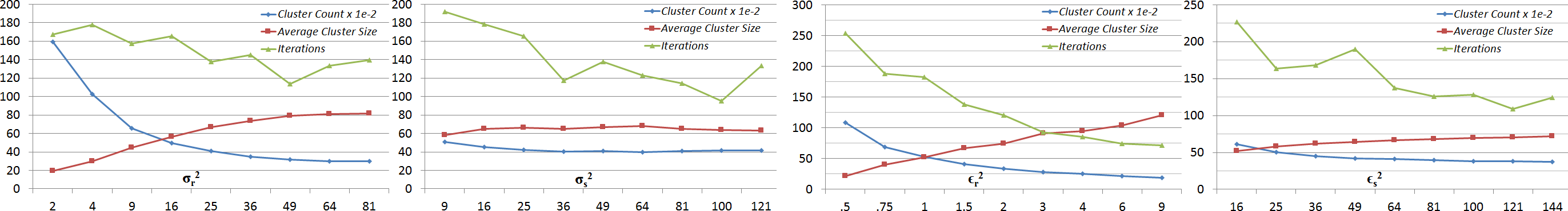
(b) Parameter sensitivity plots. Each of $\bigl{\langle}{\sigma_{base}^{r}}^{2},{\sigma_{base}^{s}}^{2},\,\epsilon_{r}^{2},\,\epsilon_{s}^{2}\bigr{\rangle}$ was varied while keeping others constant. Their effects on number of clusters, their average size, and iterations for convergence are plotted. Results were averaged over $33$ images. As with conventional MS, color domain parameters are understandably more sensitive. $\delta=.01$ was used.

Figure 2: For joint domain AAAMS over images, we show the qualitative and quantitative effects of varying the detail and vicinity parameters, $\bigl{\langle}{\sigma_{base}^{r}}^{2},{\sigma_{base}^{s}}^{2},\,\epsilon_{r}^{2},\,\epsilon_{s}^{2}\bigr{\rangle}$. Post processing was disabled, except for enforcing cluster contiguity. As can be seen, if the need be, a good control over smoothing and segmentation levels can be exercised.

2.3 Cluster Merging

For any given data points, if their mean shift trajectories intersect, they will converge to a common local mode. Thus in the vicinity of a data point’s trajectory (which is moving up some mode) - any data points in sufficient proximity, having their shift vectors deemed to be intersecting with this trajectory, could be clustered together. They will eventually end up converging on the same local mode. So we basically consider the data points in the vicinity of a cluster trajectory, $u^{\tau}$ - with an epsilon $\epsilon$, delineating the vicinity. If a data point, $y$, in vicinity is ascertained (in MergeCheck) to be heading to the same mode as $u^{\tau}$, then by transitivity - all the members of its parent cluster, $\Pi(y)$, are heading to that mode too - the clusters $u$ and $\Pi(y)$ , can then be merged. The cluster which is higher up the mode (higher density) assimilates the other cluster into itself, thus accelerating convergence to the mode. This also helps in avoiding spurious merges.

MergeCheck - This is intentionally specified as a generic function returning a true/false value. It could be implemented to suit different feature spaces and clustering criteria. The more holistic this check is, the larger the operating range of $\epsilon$ can be (assuming the distance norm holds up), without impacting clustering stability. In our experiments, we used a very lightweight generic implementation that worked well over considered data spaces - basically verifying through inner product checks that 1) relative distance between $u^{\tau+1}$ and $y$ is decreasing and 2) Mean shift bearings at $u^{\tau+1}$ and $y$ are in the same direction. We note though that divergence measures like Bhattacharya (Sec. 2.4), kernel induced feature space metrics ([26]), information-theoretic ones like Renyi’s entropy ([14]) seem viable, interesting possibilities for MergeCheck. We are yet to experiment with them.

2.4 Post Processing

Once data has been partitioned, a post processing step merges clusters with proximate modes, and ensures a minimum cluster size (in conventional Mean Shift, clusters are delineated only during the post process). Additionally for structured data, cluster contiguity could be enforced. We use graph operations. For structured data as in images, adjacency connections between clusters can be added naturally using a spatial grid structure. For unstructured data, connections between a cluster and all clusters within a reasonably large distance threshold (mode to mode distances) were added, to ensure a connected graph. Bhattacharya divergence ([2], $d_{B}$) was used as the merging criteria. It takes into account not just the variance normalized mode proximity, but also the disparity in variances themselves (Mahanalobis measure is its special case). $0\leq d_{B}\leq 4$ was a good range, with $d_{B}=1$ (somewhat analogous to $1-sigma^{2}$ disparity) performing well generally . Alg. 2 specifies the steps.

Algorithm 2 : Post Processing

 

• (For structured data only) For each cluster, use spatial adjacency to ascertain the disconnected components (highest density/mode locations for these small disconnected point sets need to be recomputed). Each disconnected component forms an additional separate cluster thereon.

• Build the adjacency graph.

• Merge all clusters which fall below minimum desired size, to the closest adjacent cluster until no such remain.

• For each remaining cluster, using its constituent points, compute the density weighted variances, similar to Eq.6 - this is representative of the cluster’s stand-alone distribution and alleviates tail influences.

• For each pair of remaining clusters $\{a,\,b\}$, connected by an adjacency edge, evaluate  $\rightarrow$ $d_{B}=\frac{1}{8}\left(\mu_{a}-\mu_{b}\right){}^{T}\left(\frac{\Sigma_{a}+\Sigma_{b}}{2}\right)^{-1}\left(\mu_{a}-\mu_{b}\right)+\frac{1}{2}ln\left(\frac{det\left(\frac{\Sigma_{a}+\Sigma_{b}}{2}\right)}{\sqrt{det\left(\Sigma_{a}\right).det\left(\Sigma_{b}\right)}}\right)$. If it falls below a certain threshold, merge the two.

Methods / Score	PRI	GCE	VoI	BDE
$AAAMS$	${\color[rgb]{1,0,0}.8230}$	${\color[rgb]{1,0,0}.1589}$	2.1785	${\color[rgb]{0,1,0}12.60}$
$JMS^{*}$	.7870	${\color[rgb]{0,1,0}.1608}$	2.2484	13.34
Prior Art [21]
$FullSpectralOverMS$ [21]	${\color[rgb]{0,1,0}0.8146}$	0.1809	${\color[rgb]{0,1,0}1.8545}$	${\color[rgb]{1,0,0}12.21}$
$JMS$ [8]	${\color[rgb]{0,0,1}0.7958}$	0.1888	${\color[rgb]{0,0,1}1.9725}$	14.41
$NCut$  [21] - Ref. [27]	0.7330	0.2662	2.6137	17.19
$MNCUT$  [21] - Ref. [6]	0.7632	0.2234	2.2789	${\color[rgb]{0,0,1}13.17}$
$GBIS$  [21] - Ref. [9]	0.7139	${\color[rgb]{0,0,1}0.1746}$	3.3949	16.67
$Saliency$  [21] - Ref. [8]	0.7758	0.1768	${\color[rgb]{1,0,0}1.8165}$	16.24
$JSEG$  [21] - Ref. [7]	0.7756	0.1989	2.3217	14.40

Table 1: Results on BSD300 [24]. We used a single parameter set $\bigl{\langle}20,36,1,64\bigr{\rangle}$ for AAAMS. For better results, $d_{B}$ was set from $\left\{.25,.5,1,1.25,1.5,2\right\}$. JMS^∗ parameters were selected per image to maintain similar segmentation levels, with an eye on preserving details, segment saliency.
For perspective, we also reproduce results from [21] of unsupervised image segmentation methods. [21] selects segment levels per image. Top three values for each index are colored as ${\color[rgb]{1,0,0}r}{\color[rgb]{0,1,0}g}{\color[rgb]{0,0,1}b}$. AAAMS performs best overall - it’s clearly ahead in PRI & GCE, and is a close second in BDE. Note that [21], which has the next best values, operates over a priori Mean Shift segmentations.

3 Results

The base scalar parameter $\sigma_{base}$, in effect, regulates the minimum desired detail in the feature space, the smoothing level. The vicinity parameter, $\epsilon$, regulates cluster merge chances and hence cluster sizes. For images, with AAAMS operating over joint domains of $\left\langle color,\,space\right\rangle$, the detail and vicinity parameters would be $\left\langle\sigma_{base}^{r},\,\sigma_{base}^{s}\right\rangle$ and $\left\langle\epsilon_{r},\,\epsilon_{s}\right\rangle$ respectively (indicated in Alg. 1). Fig. 2, shows quantitative and qualitative effects of their variation. Although a good degree of control is possible to achieve a desired result, our experiments showed that any low valued set gave nice results over a good range of images.

Due to agglomeration, the number of clusters decrease monotonically every iteration. Only a fraction of clusters remain after the first couple of iterations; with the cluster count falling rapidly in all early iterations. The scheme thus results in a drastic reduction in net mean shift computes - as compared to the hitherto style of clustering only after convergence, where computations happen for every data point, in each iteration. (for dense image data, typically less than $5\%$ of the clusters remain by the $11^{th}$ or $12^{th}$ iteration). This serves to offset the additional computational workload arising from the use of full bandwidth matrices. Our straight up joint domain implementation was achieving similar timings on average to standard Mean Shift, which uses scalar bandwidths. Improvements in efficency based on fast nearest neighbor search such as exploiting grid structure of spatial domain, locally sensitive hashing ([16]) are applicable in our methodology too. Using Gaussian kernels, with a convergence delta, $\delta$, set adequately to $.01$, merges would cease before $90^{th}$ iteration, with convergence around the $100^{th}$. When just pre-partitioning is the end objective, the merging scheme thus allows us to fine tune stopping criteria. Along with the first iteration shift vectors, globally normalized local density values at each data point were stored for consequent use too. In each iteration, $\rho(u^{\tau})$ was then approximated by the density value at $u^{\tau}$’s nearest data point. We found perturbations to be generally useful, lending to mode detection robustness and more salient partitioning. A cluster at convergence can be perturbed a fixed number of times consecutively, with progressively damped magnitudes. $u$ then, would not be brought out of contention in the next iteration - although the immediate trajectory point resulting from the perturbation will not be included in $T_{u}$. The results presented in this paper though, are with perturbations disabled.

Image                                  JMS                                 AAAMS                            JMS Labels                   AAAMS Labels

             Lady                      JMS - 523 Labels,                AAAMS - 490 Labels
             Soldier                      JMS - 617 Labels,            AAAMS - 601 Labels
             Bench                       JMS - 180 Labels,            AAAMS - 165 Labels
             Mandrill                  JMS - 752 Labels,             AAAMS - 721 Labels

Figure 3: AAAMS preserves more details and affects more perceptually salient segmentations, at similar clustering levels. We used a single parameter set, $\bigl{\langle}{\sigma_{base}^{r}}^{2},{\sigma_{base}^{s}}^{2},\,\epsilon_{r}^{2},\,\epsilon_{s}^{2}\bigr{\rangle}=\bigl{\langle}15,16,1,81\bigr{\rangle}$ with $d_{B}=1$, to show its adaptivity on varied images. JMS segments were kept around the same, with eye on preserving detail; it still smooths over at places. Its parameter values varied significantly from image to image - $\,{\sigma^{r}}^{2}\in\left[49,\,81\right]\,,\,{\sigma^{s}}^{2}\in\left[100,\,289\right]$. Minimum cluster size was 10.

Image                     JMS                    AAAMS                JMS Labels         AAAMS Labels

      Aeroplane               JMS - 14 Labels,            AAAMS - 11 Labels
      ColorWheel               JMS - 51 Labels,            AAAMS - 48 Labels
      Wasp               JMS - 150 Labels,            AAAMS - 111 Labels

Figure 4: More parsimonious segmentations were quite often not achievable with JMS - some varied examples are shown above (Images such as Lady in Fig.3 are a typical case too). Both methods were configured for reduced label usage. Minimum cluster size was 10. JMS, at its limit, is breaking boundaries and under segmenting. AAAMS with lesser labels, does not break boundaries, still maintains segment saliency.

Figure 5: Single domain clustering examples over color data (top row, 11 clusters) and simulated gaussian mixtures (second row) in 2D & 3D respectively. $1-sigma$ final trajectory-set bandwidths have been overlaid at converged mode positions.

$\mathbf{Data\leavevmode\nobreak\ \langle\#Dims,\#Classes\rangle}$	PRI	GCE	VoI
$Seeds\leavevmode\nobreak\ \leavevmode\nobreak\ \leavevmode\nobreak\ \leavevmode\nobreak\ \leavevmode\nobreak\ \langle 7D,3\rangle$	${\color[rgb]{1,0,0}.89}$ / .86 / .87	${\color[rgb]{1,0,0}.17}$ / .20 / .19	${\color[rgb]{1,0,0}0.85}$ / 0.98 / 0.93
$Yeast\leavevmode\nobreak\ \leavevmode\nobreak\ \leavevmode\nobreak\ \leavevmode\nobreak\ \leavevmode\nobreak\ \langle 8D,10\rangle$	${\color[rgb]{1,0,0}.69}$ / .61 / .67	.44 / ${\color[rgb]{1,0,0}.39}$ / .47	${\color[rgb]{1,0,0}3.03}$ / 3.10 / 3.22
$Letters\leavevmode\nobreak\ \leavevmode\nobreak\ \leavevmode\nobreak\ \langle 16D,26\rangle$	${\color[rgb]{1,0,0}.87}$ / .86 / .83	.67 / .70 / ${\color[rgb]{1,0,0}.62}$	4.96 / 5.16 / ${\color[rgb]{1,0,0}4.72}$

Table 2: Results on higher dimension real world datasets from [1], with a single kernel. Indicated values are of AAAMS / MS / VariableMS ([16]) respectively, with best values in ${\color[rgb]{1,0,0}red}$.

For image data, comparisons (Figs. 3, 4, Table. 1 ) are shown with joint domain Mean Shift implementation (JMS) from EDISON ([8]), over Berkely Segmentation Dataset ([24], BSD300). BSD300 is meant for supervised algorithms - we simply clubbed the training and test images together. For sake of completeness, prior art on unsupervised image segmentation is also shown in Table. 1. All indicated parameter values for AAAMS and JMS are squared. We did not search for the best performing parameter set for AAAMS, opting for a single low valued set instead. AAAMS performed significantly better than JMS, with results superior to other unsupervised image segmentation methods as well.

Our experiments indicated that low base bandwidths, $\left\langle\sigma_{base}^{r},\,\sigma_{base}^{s}\right\rangle$, performed generally well on a good range of images (Fig. 3). This was due to the presented approach being locally adaptive and anisotropic. At similar clustering levels, AAAMS preserved more details and affected more salient segmentations.

Single kernel AAAMS was tested on images and 2D, 3D gaussian mixtures at varied scales - with nice results. AAAMS results in Figs. 1(a), 5 are with postprocessing disabled. As indicated in Figs. 1(a), 5, reasonable local bandwidths arise, robustly identifying modes and salient clusters, by adapting according to local structure.

Experiments were conducted with some higher dimension datasets from [1] as well. Table. 2 shows initial results, along with comparisons with single domain standard Mean Shift (MS), and [16]’s isotropic variable bandwidth implementation. Cluster count was kept the same as class count. AAAMS post-processing was disabled. [16] first determines isotropic point bandwidths using the $k^{th}$ nearest neighbor distance heuristic, and subsequently utlizes them in single kernel mean shift iterations. Our experiments with it indicated a lack of clustering control. The datasets were meant for supervised classification, with attributes/feature components at different scales, and having uncorrelated and/or uninformative dimensions. Without any pre-processing (normalizations, component analysis) decent results were attained with a single kernel AAAMS. Note that [16] internally normalizes the data, while AAAMS & MS results are without any normalizations.

Promising results, both qualitative and quantitative, are indicative of the efficacy of the presented approach. We intend to experiment further, especially with different merging schemes and on varied data spaces.

4 Conclusion

A generalized methodology for feature space partitioning and mode seeking was presented - leveraging synergism of adaptive, anisotropic Mean Shift and guided agglomeration. Unsupervised adaptation of full anisotropic bandwidths is useful and further enables Mean Shift clustering. We are excited about its prospects on point-normal clouds and video streams.

Our experiments did indicate sparse data to be an issue. This is understandable, as it encumbers cluster growth and bandwidth development, with AAAMS behaving like conventional Mean Shift then. Future work would also focus on alleviating this issue.

References

- Asuncion and Newman [2007] Arthur Asuncion and David Newman. UCI machine learning repository - http://archive.ics.uci.edu/ml/, 2007.
- Bhattacharyya [1946] Anil Bhattacharyya. On a measure of divergence between two multinomial populations. Sankhyā: The Indian Journal of Statistics, pages 401–406, 1946.
- Bradski [1998] Gary R Bradski. Real time face and object tracking as a component of a perceptual user interface. In Applications of Computer Vision, 1998. WACV’98. Proceedings., Fourth IEEE Workshop on, pages 214–219. IEEE, 1998.
- Carreira-Perpiñán [2006] Miguel Á. Carreira-Perpiñán. Fast nonparametric clustering with gaussian blurring mean-shift. In Proceedings of the 23rd International Conference on Machine Learning, ICML ’06, pages 153–160, New York, NY, USA, 2006. ACM.
- Carreira-Perpiñán [2007] Miguel Á. Carreira-Perpiñán. Gaussian Mean-Shift is an EM algorithm. Pattern Analysis and Machine Intelligence, IEEE Transactions on, 29(5):767–776, 2007.
- Chacón et al. [2013] José E Chacón, Tarn Duong, et al. Data-driven density derivative estimation, with applications to nonparametric clustering and bump hunting. Electronic Journal of Statistics, 7:499–532, 2013.
- Cheng [1995] Yizong Cheng. Mean shift, mode seeking, and clustering. Pattern Analysis and Machine Intelligence, IEEE Transactions on, 17(8):790–799, 1995.
- Christoudias et al. [2002] Christopher M Christoudias, Bogdan Georgescu, and Peter Meer. Synergism in low level vision. In Pattern Recognition, 2002. Proceedings. 16th International Conference on, volume 4, pages 150–155. IEEE, 2002.
- Comaniciu et al. [2003] D. Comaniciu, V. Ramesh, and P. Meer. Kernel-based object tracking. Pattern Analysis and Machine Intelligence, IEEE Transactions on, 25(5):564–577, May 2003.
- Comaniciu [2003] Dorin Comaniciu. An algorithm for data-driven bandwidth selection. Pattern Analysis and Machine Intelligence, IEEE Transactions on, 25(2):281–288, 2003.
- Comaniciu and Meer [2002] Dorin Comaniciu and Peter Meer. Mean shift: A robust approach toward feature space analysis. Pattern Analysis and Machine Intelligence, IEEE Transactions on, 24(5):603–619, 2002.
- Comaniciu et al. [2001] Dorin Comaniciu, Visvanathan Ramesh, and Peter Meer. The variable bandwidth mean shift and data-driven scale selection. In Computer Vision, 2001. ICCV 2001. Proceedings. Eighth IEEE International Conference on, volume 1, pages 438–445. IEEE, 2001.
- Duong et al. [2008] Tarn Duong, Arianna Cowling, Inge Koch, and MP Wand. Feature significance for multivariate kernel density estimation. Computational Statistics & Data Analysis, 52(9):4225–4242, 2008.
- Erdogmus et al. [2008] Deniz Erdogmus, Umut Ozertem, and Tian Lan. Information theoretic feature selection and projection. In Speech, Audio, Image and Biomedical Signal Processing using Neural Networks, pages 1–22. Springer, 2008.
- Fukunaga and Hostetler [1975] Keinosuke Fukunaga and Larry Hostetler. The estimation of the gradient of a density function, with applications in pattern recognition. Information Theory, IEEE Transactions on, 21(1):32–40, 1975.
- Georgescu et al. [2003] Bogdan Georgescu, Ilan Shimshoni, and Peter Meer. Mean shift based clustering in high dimensions: A texture classification example. In Computer Vision, 2003. Proceedings. Ninth IEEE International Conference on, pages 456–463. IEEE, 2003.
- Horová et al. [2013] Ivana Horová, Jan Koláček, and Kamila Vopatová. Full bandwidth matrix selectors for gradient kernel density estimate. Computational Statistics & Data Analysis, 57(1):364–376, 2013.
- Jeong et al. [2005] Mun-Ho Jeong, Bum-Jae You, Yonghwan Oh, Sang-Rok Oh, and Sang-Hwi Han. Adaptive mean-shift tracking with novel color model. In Mechatronics and Automation, 2005 IEEE International Conference, volume 3, pages 1329–1333 Vol. 3, 2005. 10.1109/ICMA.2005.1626746.
- Jimenez-Alaniz et al. [2006] R.J. Jimenez-Alaniz, M. Pohi-Alfaro, V. Medina-Bafluelos, and O. Yaflez-Suarez. Segmenting brain mri using adaptive mean shift. In Engineering in Medicine and Biology Society, 2006. EMBS ’06. 28th Annual International Conference of the IEEE, pages 3114–3117, 2006.
- Ke et al. [2007] Yan Ke, Rahul Sukthankar, and Martial Hebert. Event detection in crowded videos. In Computer Vision, 2007. ICCV 2007. IEEE 11th International Conference on, pages 1–8. IEEE, 2007.
- Kim et al. [2010] Tae Hoon Kim, Kyoung Mu Lee, and Sang Uk Lee. Learning full pairwise affinities for spectral segmentation. In Computer Vision and Pattern Recognition (CVPR), 2010 IEEE Conference on, pages 2101–2108, June 2010.
- Kohli et al. [2009] Pushmeet Kohli, Philip HS Torr, et al. Robust higher order potentials for enforcing label consistency. International Journal of Computer Vision, 82(3):302–324, 2009.
- Leibe and Schiele [2004] Bastian Leibe and Bernt Schiele. Scale-invariant object categorization using a scale-adaptive mean-shift search. In Pattern Recognition, pages 145–153. Springer, 2004.
- Martin et al. [2001] David Martin, Charless Fowlkes, Doron Tal, and Jitendra Malik. A database of human segmented natural images and its application to evaluating segmentation algorithms and measuring ecological statistics. In Computer Vision, 2001. ICCV 2001. Proceedings. Eighth IEEE International Conference on, volume 2, pages 416–423. IEEE, 2001.
- Mayer and Greenspan [2009] Arnaldo Mayer and Hayit Greenspan. An adaptive mean-shift framework for mri brain segmentation. Medical Imaging, IEEE Transactions on, 28(8):1238–1250, 2009.
- Ozertem et al. [2008] Umut Ozertem, Deniz Erdogmus, and Robert Jenssen. Mean shift spectral clustering. Pattern Recognition, 41(6):1924–1938, 2008.
- Paris and Durand [2007] Sylvain Paris and Frédo Durand. A topological approach to hierarchical segmentation using mean shift. In Computer Vision and Pattern Recognition, 2007. CVPR’07. IEEE Conference on, pages 1–8. IEEE, 2007.
- Shotton et al. [2013] Jamie Shotton, Toby Sharp, Alex Kipman, Andrew Fitzgibbon, Mark Finocchio, Andrew Blake, Mat Cook, and Richard Moore. Real-time human pose recognition in parts from single depth images. Communications of the ACM, 56(1):116–124, 2013.
- Surkala et al. [2012] M. Surkala, K. Mozdren, R. Fusek, and E. Sojka. Hierarchical evolving mean-shift. In Image Processing (ICIP), 2012 19th IEEE International Conference on, pages 1593–1596, 2012.
- Šurkala et al. [2011] Milan Šurkala, Karel Mozdřeň, Radovan Fusek, and Eduard Sojka. Hierarchical blurring mean-shift. In Advances Concepts for Intelligent Vision Systems, pages 228–238. Springer, 2011.
- Unnikrishnan et al. [2007] Ranjith Unnikrishnan, Caroline Pantofaru, and Martial Hebert. Toward objective evaluation of image segmentation algorithms. Pattern Analysis and Machine Intelligence, IEEE Transactions on, 29(6):929–944, 2007.
- Vedaldi and Soatto [2008] Andrea Vedaldi and Stefano Soatto. Quick shift and kernel methods for mode seeking. In Computer Vision–ECCV 2008, pages 705–718. Springer, 2008.
- Vojir et al. [2013] Tomas Vojir, Jana Noskova, and Jiri Matas. Robust scale-adaptive mean-shift for tracking. In Image Analysis, pages 652–663. Springer, 2013.
- Wang et al. [2004] Jue Wang, Bo Thiesson, Yingqing Xu, and Michael Cohen. Image and video segmentation by anisotropic kernel mean shift. In Computer Vision-ECCV 2004, pages 238–249. Springer, 2004.
- Yang et al. [2007] Lin Yang, Peter Meer, and David J Foran. Multiple class segmentation using a unified framework over mean-shift patches. In Computer Vision and Pattern Recognition, 2007. CVPR’07. IEEE Conference on, pages 1–8. IEEE, 2007.
- Yuan et al. [2012] Xiao-Tong Yuan, Bao-Gang Hu, and Ran He. Agglomerative mean-shift clustering. Knowledge and Data Engineering, IEEE Transactions on, 24(2):209–219, 2012.
- Zhang et al. [2006] Kai Zhang, Jamesk T Kwok, and Ming Tang. Accelerated convergence using dynamic mean shift. In Computer Vision–ECCV 2006, pages 257–268. Springer, 2006.