GASP : Geometric Association with Surface Patches

Abstract

A fundamental challenge to sensory processing tasks in perception and robotics is the problem of obtaining data associations across views. We present a robust solution for ascertaining potentially dense surface patch (superpixel) associations, requiring just range information. Our approach involves decomposition of a view into regularized surface patches. We represent them as sequences expressing geometry invariantly over their superpixel neighborhoods, as uniquely consistent partial orderings. We match these representations through an optimal sequence comparison metric based on the Damerau-Levenshtein distance - enabling robust association with quadratic complexity (in contrast to hitherto employed joint matching formulations which are NP-complete). The approach is able to perform under wide baselines, heavy rotations, partial overlaps, significant occlusions and sensor noise.

The technique does not require any priors – motion or otherwise, and does not make restrictive assumptions on scene structure and sensor movement. It does not require appearance – is hence more widely applicable than appearance reliant methods, and invulnerable to related ambiguities such as textureless or aliased content. We present promising qualitative and quantitative results under diverse settings, along with comparatives with popular approaches based on range as well as RGB-D data.

I Introduction

The popularity of lasers and RGB-D cameras has led to widespread use of range and range-color images in several robotics and perception tasks. Intrinsic to several applications, is the problem of establishing data associations (as in [30, 12]) – for example, in motion estimation, SLAM, SfM, loop closure / scene detection, multi-view primitive detection and segmentation (as in [38, 30, 20, 50, 49, 45, 24, 26]). Most 3D association solutions today, either generate sparse correspondences on feature points, assuming a locally discriminative environment; or use complete point clouds to indirectly associate densely based on some form of nearest neighbors, under restricted sensor motion.

As an alternative, we present a surface patch (depth superpixel) level association scheme. Motivated by recent trends in scene understanding literature of utilizing superpixels due to representational compactness and robustness to noise, we propose an analogous model for depth superpixels - applicable over depth images acquired from generic range sensors, where appearance / color information is not necessarily available.

Ascertaining superpixel associations without making assumptions on sensor motion, scene appearance and/or structure, is indeed difficult (and to our knowledge, unsolved). Superpixel decompositions vary in each view, rendering the correspondence inexact. Besides, superpixels are defined through (and for) homogeneity – they are not uniquely discriminable by design. The problem gets complicated further, when appearance is unavailable altogether.

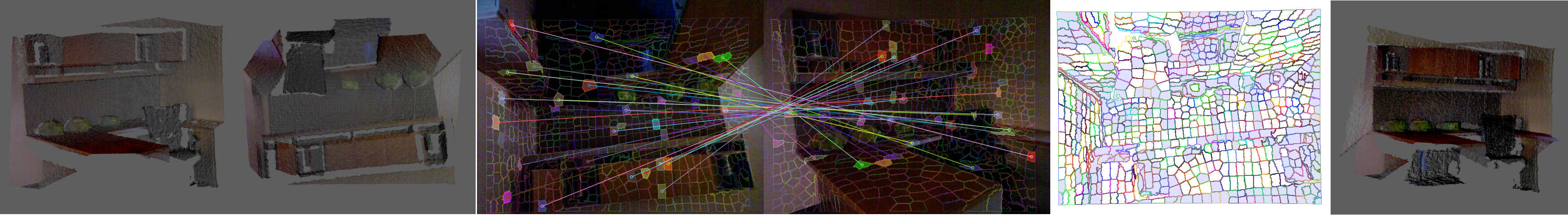
Figure 1: (Best viewed in color) Point clouds from two views of a workspace scene are shown on left. The second view was captured with the sensor completely inverted ($180^{\circ}$ roll), and from a wide baseline. The two views also have significant changes in surface resolution scales, self-occlusions, and changes in yaw & pitch. The image in centre shows a few random samples of surface patch (depth superpixel) associations between the two views, computed using our algorithm. Associated patches are connected by a line and have the same color overlay. The associations were not filtered or post-processed. The centre-right image shows the superpixel decomposition of the second view. The grey overlay over some superpixels indicates the superpixels that are not associated - these include regions which were occluded or absent in the first view. The right-most image shows the unrefined reconstruction obtained directly from the dense superpixel associations. The relative motion/transform was computed simply through corresponding 3D means of the associated superpixels.

Nevertheless such associations are very useful - because correspondent superpixels roughly represent the same physical 3D surface patch. As we will show, relative scene geometry over sufficiently large neighborhoods contains adequate discriminative information to achieve potentially dense associations. By regularizing superpixel traits such as surface area and smoothness – the associations can be made to have near co-incident 3D (centroid) localizations as well – affording nice sensor motion estimates even under significant change in perspectives and scant data acquisition (Fig. 1, Table 11). Importantly, such an approach performs equally well in locally ambiguous (such as isomorphic or textureless) or featureless environments. Furthermore, it can preserve localized semantics (encoded by the superpixel labels) across views. Although not within this article’s scope, this enables more straightforward primitive level associations and semantic transfer.

Our methodology is based on invariantly representing a (depth) superpixel through a set of relative geometrical properties/features extracted with respect to superpixels in its neighborhood. A uniquely consistent ordering is utilized to sequence this set. Such a representation is invariant to sensor’s motion, and is made robust to its noise. Our matching scheme leverages a sequence comparison metric, Restricted Damerau Levenshtein, [11] – this pertains to family of sequence alignment algorithms, [29], that have polynomial complexity, are provably optimal, and have been in popular use for large scale sequence matching, especially in bio-informatics community.

As we will show, such a scheme is physically intuitive and is naturally applicable to a geometry matching context. It is inherently robust to heavy sensor motion, significant viewpoint differences, occlusions and partial overlaps, and tolerant of match errors between superpixels, due to varying decomposition across views and sensor noise.

We evaluate our approach on ground truth datasets from [41], datasets from [50], and others collected in challenging, yet everyday settings. The experiments are indicative of the efficacy of the proposed approach in computing localized, dense associations. They also indicate more robust performance than popularly used association approaches, based on geometrical and appearance features.

II Related Work

As we are unaware of literature directly addressing our problem setting, we survey some of the relevant work in the broader scope of feature representation and data association / matching, operating over range and RGB-D data. We also refer to some pertinent literature in appearance only settings.

Point cloud association approaches based on local 3D descriptors, like ones used in [44, 37], although useful, can be potentially non-robust. They are hindered in settings which are either locally homogenous or isomorphic, which is not uncommon in everyday scenes and structures. More holistic representations have been used for association - for example, [15] accounts for partial observability of landmarks. Plane representations have been used in dominantly polygonal environments. [42, 13] tentatively associate planes between consecutive frames based on nearest neighbor descriptor matching and relative plane angles respectively, before pruning them through specialized RANSAC schemes. [47, 35] associate by assuming a physical frame to frame overlap between corresponding planes. Registration approaches such as [38, 40] require good initialization / restricted motion. [6, 25, 33] present branch and bound schemes for registration, either assuming pure rotations or known correspondences. [17, 51] present globally optimal schemes for aligning object models, utilizing local descriptors and interleaved ICP respectively.

RGB-D based dense approaches like [21, 23, 19] (and [31] which only uses depth) associate based on flow, image warping utilizing photometric errors or ICP alignment, to estimate motion. They afford sensor rotations, but operate under short baseline and under the hypothesis that associations always lie within a neighborhood epsilon. Typically, occlusions are not handled and temporal consistency is leveraged. Such methods are suitable for settings with constrained motion. [8] utilizes a patch based scheme to track deformable meshes.

RGB-D feature based approaches for more generic SLAM, SfM and motion estimation applications (as in [20, 50, 22, 34]) employ sparse image features (generally SIFT, [27]) back-projected in 3D, to ascertain frame-wise 3D correspondences. [45] augments the geometrical descriptor SHOT, [44], with texture, for improved localization and object detection.

There are higher level approaches, which associate by leveraging application specific constraints. [36] utilizes aggregation of densely sampled point features at superpixel levels for RGB-D object detection and recognition. [28] utilizes (color only) superpixel associations to reconstruct piecewise planar scenes under known extrinsics. It assumes similar sensor orientations and imposes restrictions on possible plane orientations. Stereo literature like [4, 39] ascertain disparity maps by associating surfaces / planes relying on short baselines, similar sensor orientations, and discriminative appearance or local features. [24] utilizes planar stereo reconstructs to segment fully observable foreground from multiple views. [5, 16] operate upon SfM point clouds (reconstructed a priori) to reason about visibility and association of planar primitives from multiple views. [14, 3, 18] utilize appearance similarity at patch levels to build a dictionary and associate in the nearest neighbor sense. They find use in image enhancement, and matching scenes with similar appearance.

Matching methodologies, apart from typically assuming availability of discriminative local features, quite often also rely on motion and/or visibility priors - [30] for example, performs exhaustive search over all possible permutations of joint associations (exponential complexity), and attains tractability through priors. Similarly, intractable joint probabilistic formulations used in [43, 12], attain feasibility through priors. Graph techniques have been used to ascertain jointly consistent feature matches. [10] presents a good overview – The approach is to represent features as nodes, with the relative constraints between them as graph edges. An edge preserving mapping between nodes of such graphs is then computed, as either a subgraph isomorphism, or relaxed to inexact graph homomorphism, or as bipartite graph matching problem with non-linear constraints (say, when edges are distances). All of the above formulations are NP-complete and become quickly intractable, especially in absence of priors. Exact matching formulations have been mostly limited to sparse 2D scenarios, as in [46, 2, 7], involving a rather limited number of nodes. [2] utilizes maximum common subgraph formulation to associate sparse 2D laser scans. [32] approximates a dominant solution through eigenanalysis of the graph adjacency matrix. [9, 48] present recent approximate graph based solutions for ascertaining image feature matches – [9] progressively improves skeletal graphs, while [48] employs a density maximization scheme.

III Methodology

We first segment/decompose a view into regularized depth superpixels/surface patches (Sec. III-A). Each superpixel (or the ones of interest) is then expressed through a set of geometric features/relationships arising from all the superpixels in its neighborhood. Each feature in the set corresponds to a superpixel in the considered neighborhood, and is defined through patch level relative geometrical properties expressed invariantly ($S$ec. III-B). The ascertained feature set, thus, jointly represents all geometrical features of interest in the neighborhood. Finer or coarser geometrical detail can be captured by adjusting the granularity of the superpixel decomposition. Similarly, more global (or local) geometry can be represented by considering larger (or smaller) neighborhoods.

Such a representation captures invariant 3D geometry effectively. It does not require assumptions of the scene structure, such as piecewise or dominant planarity. It is also discriminative enough to disambiguate in difficult settings such as ones with duplicate or locally isomorphic content (Fig. 4).

The feature set of a superpixel is then arranged as a sequence by enforcing an ordering over them ($S$ec. III-C). The motivation for sequencing is to induce a partial order which remains invariant across views. This is required so that feature sets from different views can be correctly matched.

Our matching scheme (Sec. III-D) utilizes edit distance based sequence comparisons ([29]), specifically the Restricted Damerau Levenshtein distance metric ([11]). The edit distance between two sequences of arbitrary length can be optimally evaluated in quadratic time, and is directly indicative of their dissimilarity. In our context, a feature sequence expresses neighborhood geometry about a given superpixel - with each of its features exclusively capturing geometric information corresponding to a neighboring surface patch. Comparisons between two such sequences, thus, gives us powerful means to ascertain the amount of geometrical mismatch between the two considered neighborhoods. The approach is also inherently robust - as scenarios with partial view overlaps, occlusions and self-occlusions are naturally afforded through the edit operations, and sensor noises can be intuitively accounted for while matching individual features in the sequences (Table II quantifies GASP’s performance with increasing baselines, perspective changes and non-overlapping content).

We specify the superpixel decomposition of given a given view of a scene as $S=\{s_{i}\}_{i=1}^{N}$. We denote $\mu\,$ ($\in S$) as the superpixel currently under consideration. Similarly, another view of the scene will have a decomposition $S^{\prime}=\{s^{\prime}_{j}\}_{j=1}^{N^{\prime}}$. $\mu^{\prime}$ would denote a superpixel from $S^{\prime}$ currently being considered for possible correspondence with $\mu$. $\aleph_{\mu}$ indicates the set of nearest superpixels in $\mu$’s 3D neighborhood, with $|\aleph_{\mu}|$ indicating the cardinality of the set. $\alpha$ refers to an arbitrary superpixel in $\mu$’s neighborhood ($\alpha\in\aleph_{\mu}$).

III-A Depth Superpixel Decomposition

Our segmentation approach essentially involves decomposing each contiguous, 3D surface (not necessarily planar), into compact (not necessarily small) smooth patches of similar surface area. The extracted superpixels thus maintain consistency across views and are uniform in 3D. We will only present a procedural overview here. A range image is first segmented into a set of contiguous components, where each component respects 3D surface edges and lies entirely on a smooth surface. This is done by comparing adjacent points for 3D connectivity, normal angles, depth disparity and utilizing curvature. Small components on/near surface edges (due to unavoidable, irregular smoothing of normals) are initially ignored and their constituent points are added through post processing. Each remaining component/surface is then decomposed into patches of similar area. This is done using K-Means with initialization seeds spread uniformly across the 3D surface (similar to [1]). Post segmentation, the remaining depth image points, and superpixels below a minimum point size are agglomerated back into the regular superpixels based on proximity and matching normals. Graph representation and operations (edge contraction, vertex splitting) are utilized for ease and ensuring superpixel contiguity. The 3D mean of a superpixel’s constituent points served as a sufficiently good location estimate. Similarly, the superpixel normal is taken as the point normals’ mean. Due to surface area regularization, parts of a scene closer to the sensor would have larger superpixels (more pixels) than the ones farther away (Fig. 2). Similarly, a view from farther away would have more superpixels, as it covers more of the scene area (Fig. 4(d)).

III-B Representing Geometry

We utilize $\aleph_{\mu}$, to express $\mu$ through a set of transformation invariant geometrical features, $Q_{\mu}=\{q_{\mu}^{\alpha}\}_{\forall\alpha\in\aleph_{\mu}}$. Each superpixel, $\alpha$, in the neighborhood, $\aleph_{\mu}$, contributes geometric information, $q_{\mu}^{\alpha}$ , and helps capture the geometry in $\mu$’s 3D neighborhood. Let $\hat{n}_{\mu}$ indicate $\mu$’s surface normal, and $l_{\mu}$ indicate its 3D location. $\overrightarrow{r}{}_{\mu}^{\alpha}=l_{\alpha}-l_{\mu}$ , would indicate the relative displacement of the superpixel; $\hat{r}{}_{\mu}^{\alpha}$ and $||\overrightarrow{r}{}_{\mu}^{\alpha}||$ would indicate its direction and magnitude respectively. Evidently, the quantities $\hat{n}_{\mu},\,\hat{n}_{\alpha},\,\overrightarrow{r}{}_{\mu}^{\alpha}$ depend on the reference frame. In order to make them invariant to the sensor pose, we express them in a coordinate frame derived from superpixels $\mu$ and $\alpha$ themselves. An orthonormal co-ordinate frame can be derived from $\hat{n}_{\mu}$ and $\overrightarrow{r}{}_{\mu}^{\alpha}$ as follows :

$$\hat{u}_{\mu}^{\alpha}=\hat{r}{}_{\mu}^{\alpha}$$ (1a)

$$\hat{v}_{\mu}^{\alpha}=\frac{\hat{n}_{\mu}-\left(\hat{n}_{\mu}\cdot\hat{r}{}_{\mu}^{\alpha}\right)\hat{r}{}_{\mu}^{\alpha}}{\left\|\hat{n}_{\mu}-\left(\hat{n}_{\mu}\cdot\hat{r}{}_{\mu}^{\alpha}\right)\hat{r}{}_{\mu}^{\alpha}\right\|}$$ (1b)

$$\hat{w}_{\mu}^{\alpha}=\frac{\hat{u}_{\mu}^{\alpha}\times\hat{v}_{\mu}^{\alpha}}{\left\|\hat{u}_{\mu}^{\alpha}\times\hat{v}_{\mu}^{\alpha}\right\|}$$ (1c)

where $\hat{u}_{\mu}^{\alpha},\,\hat{v}_{\mu}^{\alpha},\,w_{\mu}^{\alpha}$ form an orthonormal basis. This basis is almost never degenerate, as $\hat{n}_{\mu}$ and $\overrightarrow{r}{}_{\mu}^{\alpha}$ are rarely co-linear. $\hat{n}_{\alpha}$ can now be expressed in this local frame through the projection components $[\hat{n}_{\alpha}\cdot\hat{u}_{\mu}^{\alpha},\,\hat{n}_{\alpha}\cdot\hat{v}_{\mu}^{\alpha},\,\hat{n}_{\alpha}\cdot\hat{w}_{\mu}^{\alpha}]^{T}$. For two given superpixels, $\mu$ and $\alpha$, these components would remain independent of the sensor viewing frame. Additional pieces of relative, invariant information can be extracted through $\hat{n}_{\mu},\hat{\,n}_{\alpha}$ and $\overrightarrow{r}{}_{\mu}^{\alpha}$ as follows:

$$\theta_{\alpha,\mu}=cos^{-1}\left(\hat{n}_{\mu}\cdot\hat{n}_{\alpha}\right)$$ (2a)

$$\theta_{r,\mu}=cos^{-1}\left(\hat{r}{}_{\mu}^{\alpha}\cdot\hat{n}_{\mu}\right)$$ (2b)

$$\theta_{r,\alpha}=cos^{-1}\left(\hat{r}{}_{\mu}^{\alpha}\cdot\hat{n}_{\alpha}\right)$$ (2c)

$q_{\mu}^{\alpha}$ can now be expressed as a feature vector constituting of seven relative, invariant elements. We have then :

$$q_{\mu}^{\alpha}=\left[\right.||\overrightarrow{r}{}_{\mu}^{\alpha}||\cdot sgn(\hat{n}_{\alpha}\cdot\hat{u}_{\mu}^{\alpha}),\leavevmode\nobreak\ ||\overrightarrow{r}{}_{\mu}^{\alpha}||\cdot sgn(\hat{n}_{\alpha}\cdot\hat{v}_{\mu}^{\alpha}),\dots{\\ }\dots||\overrightarrow{r}{}_{\mu}^{\alpha}||\cdot sgn(\hat{n}_{\alpha}\cdot\hat{w}_{\mu}^{\alpha}),\leavevmode\nobreak\ ||\overrightarrow{r}{}_{\mu}^{\alpha}||,\leavevmode\nobreak\ \theta_{\alpha,\mu},\leavevmode\nobreak\ \theta_{r,\mu},\leavevmode\nobreak\ \theta_{r,\alpha}\left.\right]^{T}$$ (3)

where $||\overrightarrow{r}{}_{\mu}^{\alpha}||$ is included for additional redundancy. We utilize the signs of $\hat{n}_{\alpha}$’s projection components (with $sgn(.)\in\{-1,0,1\}$), as their actual values tend to be noisy. A proper approach is to utilize an epsilon-insensitive signum function, for example $sgn_{e}(.)$ rather than $sgn(.)$ - it is defined as zero either when $1)$ the angle between $\hat{n}_{\alpha}$ and the respective basis vector $\not\in[e_{\theta},\,PI-e_{\theta}]$; or in the uncommon case of degenerate basis when $2)$ $\hat{n}_{\mu}$ is co-linear with $\overrightarrow{r}{}_{\mu}^{\alpha}$ (that is, when $\theta_{r,\mu}\not\in[e_{\theta},\,PI-e_{\theta}]$). $e_{\theta}$ is the allowable angular noise tolerance. The component signs are then scaled by $||\overrightarrow{r}{}_{\mu}^{\alpha}||$ in order to incorporate signed distance information between $\mu$ and $\alpha$. The feature, $q_{\mu}^{\alpha}$, is thus expressed stably in presence of noises. It captures relative information between $\mu$ and the neighborhood superpixel $\alpha$ – the relative pose, distance, orientation and bearings. Understandably, the elements of $q_{\mu}^{\alpha}$ would be affected by noise. However, our matching methodology is robust to it, explicitly accounts for it ($Sec.$ III-D, deviation thresholds). The joint feature set $Q_{\mu}=\{q_{\mu}^{\alpha}\}_{\forall\alpha\in\aleph_{\mu}}$, constituting of relative feature vectors from all superpixels in $\aleph_{\mu}$, thus, essentially expresses the geometry in $\mu$’s neighborhood invariantly.

III-C Ordering

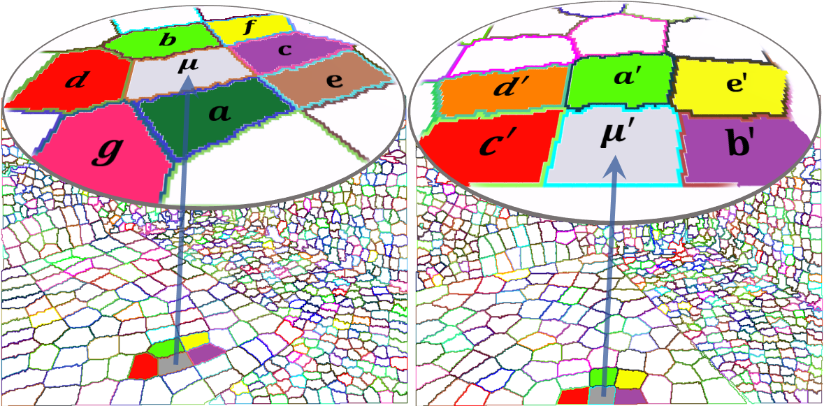
Figure 2: Illustrative consistent orderings of immediate neighborhoods of associating superpixels, $\mu$ and $\mu^{\prime}$ are shown. The orderings are indicated by alphabetical progression of the marked neighboring superpixels. The matching pairs of superpixels are shown on the table, and share a common color. The orderings are consistent as the sets of corresponding neighborhood superpixels {b, c, d, f} and {a’, b’, c’, e’}, as indicated by their increasing alphabetic order, arise identically in the orderings.

Once the geometric feature set has been determined, a partial ordering needs to be imposed on its elements to obtain a feature sequence - as our matching scheme leverages a distance metric based on sequence aligning comparisons. An ordering over $\mu$’s neighborhood $\aleph_{\mu}$, can be denoted as $\overset{\leftharpoonup}{O}_{\mu}=\left\langle a,b,c\dots\alpha\dots\right\rangle,\,\forall\alpha\in\aleph_{\mu}$ – where $\left\langle a,b,c\dots\right\rangle$ indicates the ordered sequence of superpixels. This is used to order the joint feature set $Q_{\mu}$ as $\overset{\leftharpoonup}{Q_{\mu}}=\left\langle q_{\mu}^{a},q_{\mu}^{b},q_{\mu}^{c}\dots q_{\mu}^{\alpha}\dots\right\rangle$. These ordered sequences are subsequently utilized to ascertain a potential association between two given superpixels, $\mu\,\&\,\mu^{\prime}$ from different views. The approach is to devise an ordering scheme such that two superpixel orderings, $\overset{\leftharpoonup}{O_{\mu}\,}\&\,\overset{\leftharpoonup}{O_{\mu^{\prime}}}$ (over $\aleph_{\mu}\,\&\,\aleph_{\mu^{\prime}}$) are both partially ordered by (with respect to) their matching subsequences - these subsequences would be the identically ordered (sub-)sets of corresponding superpixels in neighborhoods of $\mu$ and $\mu^{{}^{\prime}}$ respectively. To put it simply, the order of the correctly corresponding superpixels in the neighborhoods $\aleph_{\mu}$ and $\aleph_{\mu^{\prime}}$ respectively, should remain invariant in the respective orderings, $\overset{\leftharpoonup}{O_{\mu}}$ and $\overset{\leftharpoonup}{O_{\mu^{\prime}}}$ ($\overset{\leftharpoonup}{O_{\mu}}$ and $\overset{\leftharpoonup}{O_{\mu^{\prime}}}$ should be consistent). Fig. 2 illustrates consistent orderings, $\overset{\leftharpoonup}{O}_{\mu}=<a,b,c,d,e,f,g>$ and $\overset{\leftharpoonup}{O}_{\mu^{\prime}}=<a^{\prime},b^{\prime},c^{\prime},d^{\prime},e^{\prime}>$, over immediate neighborhoods of two correctly associating superpixels $\mu$ and $\mu^{\prime}$. These orderings are mutually consistent as the correct correspondences in the neighborhoods form subsequences – $<b,c,d,f>$ and $<a^{\prime},b^{\prime},c^{\prime},e^{\prime}>$ arise in identical order in $\overset{\leftharpoonup}{O}_{\mu}$ and $\overset{\leftharpoonup}{O}_{\mu^{\prime}}$ respectively.

To achieve ordering consistency, we utilize $Q_{\mu}$ itself which already constitutes of a superpixel-wise set of invariant geometric features relative to $\mu$. In effect, $\overset{\leftharpoonup}{Q_{\mu}}$ is simply ascertained through a robust sorting operation over $Q_{\mu}$’s elements ($\{q_{\mu}^{\alpha}\}$, which are invariant). Note that since this ordering is derived from geometry with respect to $\mu$ (Eqs. 1, 2), it will not, in general, be consistent with an ordering over an arbitrary superpixel from $S^{\prime}$. It will only be consistent with an ordering, say $\overset{\leftharpoonup}{O}_{\mu^{\prime}}$, defined about some superpixel $\mu^{\prime}$ in $S^{\prime}$, which has similar relative geometry in its neighborhood as $\mu$ – which is precisely the objective. Thus $\overset{\leftharpoonup}{Q_{\mu}}=Sort(Q_{\mu},\,e_{r},\,e_{\theta})$; with the sorter conducting pairwise comparisons between $Q_{\mu}$’s constitutent features. The second dimension (of the two features being compared) is only used if the first dimension is equivalent, the third dimension is only used if the first two are equivalent, and so forth. Equivalence is defined as the values being within epsilon tolerances of each other, to affect resolution, and account for noise and finite precision numerical errors. A distance tolerance, $e_{r}$ is used, along with the afore-utlilized angular tolerance, $e_{\theta}.$ In our experiments over noisy Kinect data, $e_{r}=.02$ metres and $e_{\theta}=\nicefrac{{5\pi}}{{180}}$ radians, worked well.

Algorithm 1 Compare Geometric Sequences

1:Function  CompareRDL( $\overset{\leftharpoonup}{Q_{\mu}},\overset{\leftharpoonup}{Q_{{\mu}^{\prime}}}$ )    Returns $D_{RDL}(\mu,\mu^{\prime})$

2:     $insert\leftarrow 1;\leavevmode\nobreak\ delete\leftarrow 1;$

3:     $replace\leftarrow\infty;\leavevmode\nobreak\ switch\leftarrow 0;$

4:     $L_{\mu}\leftarrow|\overset{\leftharpoonup}{Q_{\mu}}|;\leavevmode\nobreak\ L_{{\mu}^{\prime}}\leftarrow|\overset{\leftharpoonup}{Q_{{\mu}^{\prime}}}|;$

5:     $tab(1,1)\leftarrow 0;$

6:     For Each $i\in[2,L_{\mu}]$ 

7:         $tab[i,1]\leftarrow tab[i-1,1]+insert$

8:     End For

9:     For Each $j\in[2,L_{{\mu}^{\prime}}]$ 

10:         $tab[1,j]\leftarrow tab[1,j-1]+delete$

11:     End For

12:     For Each $j\in[2,L_{{\mu}^{\prime}}]$ 

13:         For Each $i\in[2,L_{\mu}]$ 

14:              if $Match(\overset{\leftharpoonup}{Q_{\mu}}(i),\overset{\leftharpoonup}{Q_{{\mu}^{\prime}}}(j))$ 

15:                  $\leavevmode\nobreak\ \leavevmode\nobreak\ substitute\leftarrow 0$

16:              else$\leavevmode\nobreak\ \leavevmode\nobreak\ substitute\leftarrow replace$               

17:              $tab[i,j]\leftarrow min\Biggl{\{}\begin{array}[]{c}tab[i-1,j]+insert,\\ tab[i,j-1]+delete,\\ tab[i,j-1]+substitute\end{array}\Biggr{\}}$

18:              if $i>2\leavevmode\nobreak\ \&\leavevmode\nobreak\ j>2\leavevmode\nobreak\ \&\leavevmode\nobreak\ Match(\overset{\leftharpoonup}{Q_{\mu}}(i-1),\overset{\leftharpoonup}{Q_{{\mu}^{\prime}}}(j-1))$ 

19:                  $\leavevmode\nobreak\ \leavevmode\nobreak\ tab[i,j]\leftarrow min(tab[i,j],tab[i-2,j-2]+switch)$               

20:         End For

21:     End For

22:   Return $tab[L_{\mu},L_{\mu^{\prime}}]$

23:End Function

1:Function  Match($\leavevmode\nobreak\ q^{\beta},\leavevmode\nobreak\ q^{\gamma}\leavevmode\nobreak\$)    Returns $True\leavevmode\nobreak\ or\leavevmode\nobreak\ False$

2:     $r_{dev}\leftarrow UserDefined;\leavevmode\nobreak\ \theta_{dev}\leftarrow UserDefined;$

3:     $q_{noise}\leftarrow[\theta_{dev},\theta_{dev},\theta_{dev},r_{dev},r_{dev},r_{dev},r_{dev}]$

4:     $\Delta q\leftarrow abs(q^{\beta}-q^{\gamma})$

5:     For Each $t\in[1,7]$ 

6:         if $\Delta q[t]>q_{noise}[t]$ 

7:              Return $False$          

8:     End For

9:   Return $True$

10:End Function

III-D Matching

A pair of superpixels, $\mu$ and $\mu^{\prime}$, can now be compared for geometric correspondence using their respective ordered feature sequences $\overset{\leftharpoonup}{Q_{\mu}}$ and $\overset{\leftharpoonup}{Q_{\mu^{\prime}}}$. We utilize a sequence matching scheme based on [11], to ascertain/quantify the dissimilarity between the sequences in the form of edit distances. Edit distance based algorithms, [29], operate by editing one sequence into another. By utilizing efficient dynamic programming, they progressively compare two elements at a time, one from each sequence. If the elements match up, the next pair of elements is considered – else element in one of the sequences is edited first at a cost (typically by inserting, deleting or replacing it), before resuming the comparisons. Sequences which have matching elements will result in lower edit distances than ones which do not. Additionally, sequences which have matching elements in the same order will result in lower edit distances than ones which do not. The computed distances for algorithms such as [11] are optimal with respect to the specified editing costs.

Two features, $q_{\mu}^{\alpha}$ and $q_{\mu^{\prime}}^{\alpha^{\prime}}$, from the respective sequences $\overset{\leftharpoonup}{Q_{\mu}}$ and $\overset{\leftharpoonup}{Q_{\mu^{\prime}}}$, will match up when relative geometry of patch $\alpha$ with respect to $\mu$ , is the same as the relative geometry of $\alpha^{\prime}$ with respect to $\mu^{\prime}$ ($q_{\mu}^{\alpha}$ and $q_{\mu^{\prime}}^{\alpha^{\prime}}$ would then hold approximately same values). If $\mu$ and $\mu^{\prime}$ have the same relative geometry in their neighborhoods, the sequences on the whole will naturally match, and will not require many edit operations – resulting in low edit distances; else the distances will be high. Additionally, by devising an ordering utilizing the unique relative features themselves, two sequences which do not capture similar geometry will match up badly, because their ordering will differ significantly. We utilize the Restricted Damerau–Levenshtein (RDL, [11]) algorithm for ascertaining sequence disparity. In contrast to the popular Levenshtein algorithm ([29]), which allows insert, delete and replace operations over sequence elements, RDL allows the additional operation of transposition of adjacent elements , and has the additional constraint that each subsequence can be edited only once. The edit operations’ costs can be set arbitrarily to suit a use case, and to achieve a desired resolution. Comparing two sequences through RDL is a symmetric operation, and sequences of different sizes can be compared.

These properties suit our needs nicely. Superpixels in the neighborhood $\aleph_{\mu}$ may not be present in $\aleph_{\mu^{{}^{\prime}}}$ and vice versa. This would be because of partial overlap of content between views, and because of occlusions. The operations of insert and delete will basically edit such non-matching features from the sequences. The ability to transpose adjacent features accounts for slight errors in the sequence orderings. Replacement in this context, being physically meaningless, is disabled. Also, the restriction that each subsequence can be altered only once, prevents any re-edits over incumbent feature alignments. Insertion, deletion are symmetric operations and we nominally set their cost to unity. Transposition cost is set to zero, as it only occurs only due to slight ordering inconsistencies.

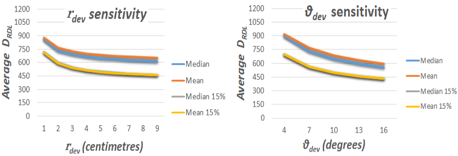
Figure 3: Impact of varying match thresholds $r_{dev}\leavevmode\nobreak\ \&\leavevmode\nobreak\ \theta_{dev}$ on averaged $D_{\mu_{RDL}}$ is shown. Default $r_{dev}$, $\theta_{dev}$ were $5$ cm and $10^{\circ}$. Mean and Median edit distances, over all associations, and over top $15\%$ are shown.

Obtaining a match between two given features, $q_{\mu}^{\alpha}$ and $q_{\mu^{\prime}}^{\alpha^{\prime}}$, while comparing $\overset{\leftharpoonup}{Q_{\mu}}$ and $\overset{\leftharpoonup}{Q_{\mu^{\prime}}}$ is easy. Basically, a match is established when the respective components of the two features lie within some acceptable range of each other. Two simple, intuitive thresholds – one for allowable angular deviation, $\theta_{dev}$ and the other for allowable distance deviation, $r_{dev}$ – are utilized. These thresholds account for noise and allowable slack in elements of $q_{\mu}^{\alpha}$ and $q_{\mu^{\prime}}^{\alpha^{\prime}}$. Fig. 3 plots the effect of varying them on (average) edit distances. Also, more precise, co-incident localizations can be achieved by considering smaller values, and a more granular superpixel discretization (vice versa is applicable too).

Two superpixel sequences from different views corresponding to the same 3D location, should have zero edit costs – assuming complete overlap of neighborhoods, no occlusions and consistent segmentations. In practice, correctly associated superpixels (their sequences) would still have some edit costs due to partially overlapping neighborhood geometry, occluded regions, and inexact superpixel decomposition across views. Desirably, these absent, occluded, or mismatched superpixel features would be edited out. Incorrect associations will have significantly higher edit distances, as a consequence of dissimilar neighborhood geometry. Alg. 1 specifies the matching algorithm. It returns the net edit cost, $D_{RDL}(\mu,\mu^{\prime})$, between the feature sequences of $\mu$ and $\mu^{\prime}$, being considered for association. For clarity, embellishments for memory and computational efficiency have been left out. Note that $D_{RDL}(\mu,\mu^{\prime})\equiv D_{RDL}(\mu^{\prime},\mu)$.

III-E Ascertaining Associations

The best potential, putative association for a superpixel, $\mu\in S$ , would be the superpixel in $S^{\prime}$ whose neighborhood geometry matches most with $\mu$’s neighborhood - one whose feature sequence gives the lowest edit distance with $\overset{\leftharpoonup}{Q_{\mu}}$.

$$D_{\mu_{RDL}}=min_{\forall\alpha^{\prime}\in S^{\prime}}(D_{RDL}(\mu,\alpha^{\prime}))$$ (4)

where $D_{\mu_{RDL}}$ indicates the edit distance from the best association in $S^{\prime}$, $\mu_{best}^{\prime}\equiv argmin_{\forall\alpha^{\prime}\in S^{\prime}}(D_{RDL}(\mu,\alpha^{\prime}))$. $D_{\mu_{RDL}}$is basically indicative of the amount of rigid geometry mismatch between the neighborhoods of $\mu$ and its best putative association; and can hence be utilized to ascertain whether the putative association is considered correct. Normalized edit distances are used for this purpose. For view to view matching, all superpixels in a view can be made to use equal size neighborhoods (that is, the set of nearest superpixels in 3D) ; thus $|\aleph_{\mu}|=k_{S},\leavevmode\nobreak\ \forall\mu\in S$ and $|\aleph_{\mu^{\prime}}|=k_{S^{\prime}},\leavevmode\nobreak\ \forall\mu^{\prime}\in S^{\prime}$. $D_{RDL}(\mu,\mu^{\prime})$, for any $\mu$ and $\mu^{\prime}$, can thus have a maximum value of $(k_{S}+k_{S^{\prime}})$, assuming unit costs for insert/delete operations. Normalized edit distance is then obtained as :

$$\hat{D}_{\mu_{RDL}}=\frac{min_{\forall\alpha^{\prime}\in S^{\prime}}(D_{RDL}(\mu,\alpha^{\prime}))}{(k_{S}+k_{S^{\prime}})}$$ (5)

$D_{\mu_{RDL}}/\hat{D}_{\mu_{RDL}}$ are dependable measures of association quality. A putative association for a given superpixel, $\mu$, is considered correct in the geometric sense, if $\hat{D}_{\mu_{RDL}}$ is not more than a given normal gating value, $\lambda\in\left[0,1\right]$ ($\hat{D}_{\mu_{RDL}}\leq\lambda$ for association). A lower $\lambda$ would result in more confident and localized associations, while denser but possibly coarser associations would arise at higher $\lambda$ gatings (depending on a scene’s geometrical ambiguity, considered neighborhood sizes and match deviation thresholds).

# Feature means queried - C	$25$	$50$	$75$	$100$
$\mathbf{\mu_{best}^{\prime}}$ found (% Avg., $\mathbf{\lambda=.5}$)	$71.5$	$86.8$	$94.5$	$98.9$

Table I: Averaged % of best associations with increasing query sizes.

Obtaining a putative association, when comparing with all superpixels in $S^{\prime}$, would have a worst case complexity of $O(||S^{\prime}|k_{S}k_{S^{\prime}}|)$. Although the cubic complexity is tractable, significant further improvements are possible. Some discriminative information can be leveraged from the feature set, $Q_{\mu}$’s mean, $\overline{Q}_{\mu}$. If two superpixels, $\mu$ and $\mu^{\prime}$ form a correct correspondence, their respective feature set averages, $\overline{Q}_{\mu}$ and $\overline{Q}_{\mu^{\prime}}$ would be close to each other. To find the putative match for $\mu$ in $S^{\prime}$, we therefore build a KD-tree over feature set means (normalized) of all superpixels in $S^{\prime}$, and search/query for $C$ of the nearest neighboring feature set means to $\overline{Q}_{\mu}$. The putative association, and subsequently a possible correct association for $\mu$, is then ascertained from the superpixels corresponding to these queried feature means rather than considering all superpixels in $S^{\prime}$. This brings down the complexity of ascertaining a putative association to quadratic – $O(Ck_{S}k_{S^{\prime}})$, where $C$ is the constant number of queries, with $C\ll S^{\prime}$. Table I indicates the average percentage of best associations ($\mu_{best}^{\prime}$) found, as a function of query size, $C$ – at least an order of magnitude reduction in computations is achieved, without any significant impact on association accuracies. An early termination criteria in Alg. 1 gives another significant improvement. Since associations with normalized distances above $\lambda$ are anyways ignored, Alg. 1 can be terminated prematurely as soon as the edit costs exceed $\lambda(k_{S}+k_{S^{\prime}})$. This is generally the case for a majority of potential associations in $S^{\prime}$, and results in significant gains in practice. Further gains are possible, like screening of possible associations before computing $D_{RDL}$, utilizing progressive rigid transform estimates. Also note that the associations are computable in parallel - such kinds of efficiency gains is a subject of ensuing work.

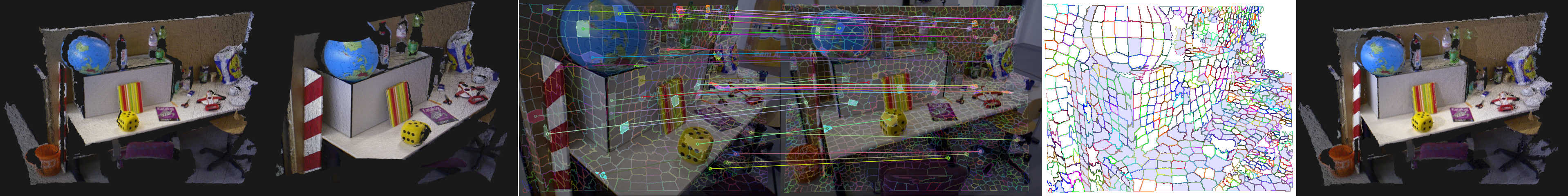
(a) Clutter scene from [41]. It has complex geometry and self-occlusions. The views have significant change in perspective, surface resolution scales.                   

(b) Scene with multiple primitive instances in a near symmetrical setting (points outside the sofa setting volume were clipped off). The views have a full roll inversion, and changes in pitch and yaw as well.

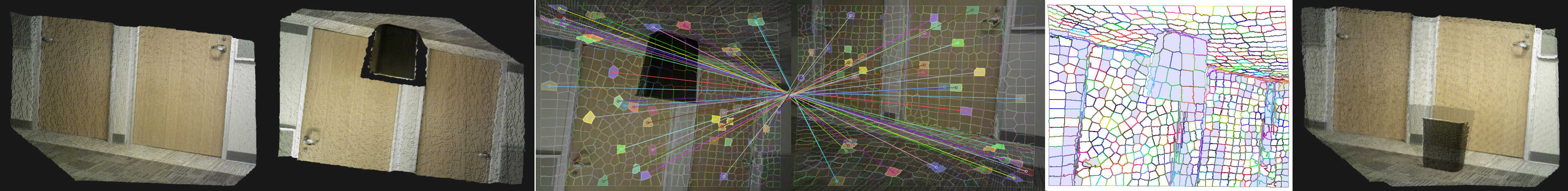
(c) Results over a scene with sparse structure and duplicate primitives. The views have a full roll inversion. An occluding body was introduced in the second view - the superpixels pertaining to it will not get matched (grey overlay).

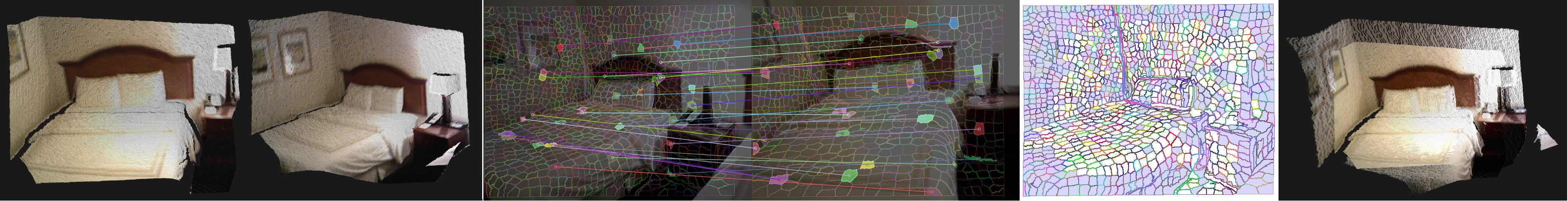
(d) Results over a scene from UMD-Hotel dataset from [50]. The views have significant change in perspective, surface resolution scale, and a partial overlap.

(e) Results over a conference room scene from Harvard-C11 dataset from [50]. The views have self-occlusion and partially overlapping geometry.             

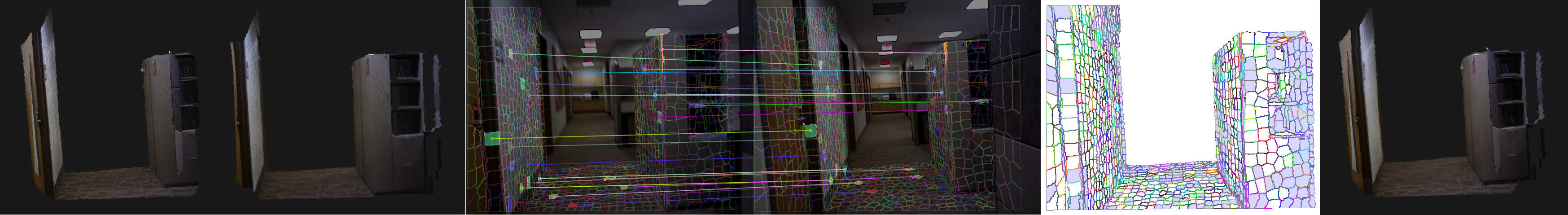
(f) Results over a corridor scene from Brown-BM1 dataset from [50].                                                                                                                              

Figure 4: Example results over varied scenes are shown. These are over different structural settings, and involve varied occlusion, overlap and sensor motion scenarios. Similar presentation and evaluation semantics as in Fig. 1 have been used. Only a sparse sampling of the ascertained associations are indicated in the figures. The achieved associations are nicely localized and densely span the scenes’ structures. These include associations over regions which have ambiguous or indiscriminate local geometry (and would prove difficult to associate otherwise).

IV Experiments And Results

We show results on datasets available from [41, 50], as well as ones collected from everyday scenes - these cover a diverse and challenging range of settings (Figs. 1, 4, Table II).

For the experiments in the article, due to the nature of datasets and to maintain uniformity, full neighborhoods were considered throughout ($k_{S}=|S|,\,k_{S^{\prime}}=|S^{\prime}|$). Smaller neighborhoods suffice for settings with locally anisomorphic content though – such as ones with clutter. The superpixel count varied between datasets, and from view to view (due to regularization) - the average number of superpixels per view was around 750. KD-tree queries, $C$, were at kept at $75$. The deviation thresholds, $\theta_{dev}\,\&\,r_{dev}$, were $10^{\circ}\,\&\,.04m$ respectively.

Exemplar qualitative results are shown in Figs. 1, 4 - the captions include some major points of note. Nicely localized associations, densely covering the scenes’ structures, were achieved - this is also indicated by the quality of unrefined reconstructions resulting from them. As the grey overlays indicate, the occluded and absent parts always get edited out – do not get matched. GASP was able to handle occlusion and partial overlap scenarios, even under sharp sensor motion. Our experiments indicated the associations obtained at low gating values to be accurate. Relatively coarser (but qualitatively correct) associations would arise at higher gating values, with incorrect associations arising mostly at high $\lambda$ gatings.

We also try to establish the localization precision of GASP’s associations, and its robustness under large sensor motions, through quantitative evaluations and comparisons for transform estimation accuracies (Table. II). Due to space constraints, the evaluation details and some points of note have been specified within the caption itself. For automation, roughly chosen high gating values were used ($\lambda\in\{.65,\leavevmode\nobreak\ ,.65,\leavevmode\nobreak\ .8\},$ respectively for the three datasets), and the ensuing associations were subsequently filtered for 3D consistency through RANSAC - by simply utilizing the associated superpixels’ locations/means as point correspondences. Note that since we ascertain superpixel level associations, better transformation estimates could have been obtained by utilizing richer constraints such as surface patch orientations and overlap - these were not leveraged in experiments. GASP gave consistently accurate results, under increasingly large sensor motions and in varied structural settings. It performed favorably, in comparisons with other popular approaches.

$Datasets\leavevmode\nobreak\$[41]		$Cabinet-SparseStructure$				$Structure-NoTexture$				$Household-Clutter$
$FramesSkipped$		$10$	$20$	$30$	$40$	$25$	$50$	$75$	$100$	$10$	$50$	$100$
$\begin{array}[]{c}Trans_{RMSE}\\ (metres)\end{array}$	$GASP$	0.057	0.075	0.070	0.073	0.026	0.037	0.038	0.039	0.023	0.028	0.058
	$SHOT$	0.184	0.281	0.352	0.461	0.132	0.228	0.309	0.461	0.033	0.191	0.347
	$FPFH$	0.185	0.424	0.393	0.435	0.164	0.202	0.275	0.406	0.045	0.260	0.606
	$C-SHOT$	0.157	0.255	0.363	0.487	0.100	0.213	0.300	0.362	0.030	0.061	0.236
	$SIFT$	0.201	0.285	0.405	0.468	0.046	0.059	0.098	0.198	0.014	0.029	0.095
	$D-SIFT$	0.131	0.178	0.246	0.242	0.030	0.042	0.191	0.182	0.019	0.138	0.425
$\begin{array}[]{c}Rot_{RMSE}\\ (degrees)\end{array}$	$GASP$	1.656	1.971	2.737	2.596	0.802	0.998	1.157	1.186	1.471	1.077	2.359
	$SHOT$	4.582	9.714	9.166	13.195	4.392	7.226	8.860	9.896	1.973	6.235	14.494
	$FPFH$	5.375	11.375	10.146	11.671	5.334	6.729	7.764	14.748	2.157	8.656	22.387
	$C-SHOT$	4.359	7.678	9.231	11.666	4.177	7.212	10.571	8.592	1.511	2.775	10.927
	$SIFT$	5.140	3.764	9.090	10.287	1.436	1.908	3.226	4.863	0.531	1.113	4.819
	$D-SIFT$	3.175	4.578	5.930	6.811	1.315	1.790	6.302	6.228	0.783	5.169	21.234
$Fail\,Rate$	$GASP$	0%	0%	0%	0%	0%	0%	0%	7.14%	0%	0%	0%
	$SHOT$	7.32%	17.07%	16.67%	25.00%	0%	3.33%	20.69%	39.29%	0%	9.30%	54.29%
	$FPFH$	1.22%	7.32%	11.11%	27.50%	3.23%	3.33%	17.24%	32.14%	0%	0%	45.71%
	$C-SHOT$	8.54%	2.44%	12.96%	15.00%	3.23%	3.33%	3.45%	17.86%	0%	4.65%	28.57%
	$SIFT$	47.56%	58.54%	61.11%	67.50%	3.23%	3.33%	13.79%	21.43%	0%	0%	0%
	$D-SIFT$	1.22%	0%	1.85%	2.50%	0%	0%	0%	0%	0%	6.98%	34.29%

Table II: We demonstrate the localization accuracy of GASP’s superpixel associations by utlizing them for motion estimates, over kinect datasets from [41] which have ground truths obtained from a motion-capture system. Translation & Rotation $RMS$ errors and failure rates are shown. For all metrics, lower values are better. Since the datasets had small inter-frame motions, we skipped frames uniformly, starting from regularly spaced initial frames, to simulate significant changes in scene perspectives, sensor baselines and non-overlapping content. The datasets cover different settings - the first two are over varied structural settings with sparse local information, while the last one is over cluttered household/office settings (Fig. 4(a)). As can be seen, the transform estimates from GASP associations are accurate. They remain consistent under increasing frame skips, and with minimal failures.
  We compare with geometric as well as appearance based 3D feature approaches (ones below short solid lines), in popular use today. $SHOT$ , $FPFH$ ([44, 37]) are point based 3D descriptors based on local geometry; $C-SHOT$ additionally utlizes color information. Dense keypoints ($>2500$) for them were evaluated by volumetrically downsampling the point clouds. Standard $SIFT$ ([27]) was utilized, by back-projecting its keypoints in 3D - this is prevalent in RGBD based SfM, SLAM approaches ([50, 20]). For Dense SIFT, keypoints were taken with a step size of $8$ pixels, at $3$ scales (${1,3,9}$). For all methods, the final feature matches were ascertained by filtering for transformation consistency using RANSAC. We tried dense cloud based direct estimation techniques ([38, 23]), but they required short sensor displacements to operate properly. Top values are ordered as ${\color[rgb]{1,0,0}r}{\color[rgb]{0,1,0}g}{\color[rgb]{0,0,1}b}$. GASP performed best overall. Its associations gave significantly better motion estimates than geometric feature approaches (whose performance deterioted with increasing sensor motion). It also performed better than appearance based approaches, especially under larger sensor motions and, in settings with little texture.

V Conclusion

We presented a practical and effective approach towards the problem of dense superpixel-level data association across views, without requiring appearance sensing / information. Our approach involved an invariant representation of relative geometry over superpixel neighborhoods, and a partial ordering over them - unique to the represented geometry itself. Robust Damerau-Levenshtein edit distance was leveraged for matching these ordered representations. The approach exhibited intrinsic robustness to sensor noise and inexact superpixel decomposition across views. It was able to perform in settings with wide baselines, occlusions, partial overlap and significant viewpoint changes. Promising experiment results were achieved in varied and difficult setups.

The approach holds further potential in other applications such as transferring the semantic labels from one view to another, structure and primitive detection, and co-segmentation. These will be explored in the future, as well as improvements in the algorithm by leveraging appearance, and performing experiments in more challenging datasets.

References

- [1] D. Arthur and S. Vassilvitskii. K-Means++: The advantages of careful seeding. In ACM-SIAM symposium on Discrete algorithms, 2007.
- [2] T. Bailey, E. M. Nebot, J. Rosenblatt, and H. F. Durrant-Whyte. Data association for mobile robot navigation: A graph theoretic approach. In Robotics and Automation (ICRA), 2000.
- [3] C. Barnes, E. Shechtman, D. B. Goldman, and A. Finkelstein. The generalized patchmatch correspondence algorithm. In ECCV. 2010.
- [4] M. Bleyer, C. Rother, and P. Kohli. Surface stereo with soft segmentation. In Computer Vision and Pattern Recognition (CVPR), 2010.
- [5] A. Bodis-Szomoru, H. Riemenschneider, and L. V. Gool. Fast, approximate piecewise-planar modeling based on sparse structure-from-motion and superpixels. In Computer Vision and Pattern Recognition, 2014.
- [6] A. J. P. Bustos, T.-J. Chin, and D. Suter. Fast rotation search with stereographic projections for 3D registration. In Computer Vision and Pattern Recognition (CVPR), 2014.
- [7] T. Caelli and T. Caetano. Graphical models for graph matching: Approximate models and optimal algorithms. Pattern Recognition Letters, 2005.
- [8] C. Cagniart, E. Boyer, and S. Ilic. Probabilistic deformable surface tracking from multiple videos. In Computer Vision - ECCV. 2010.
- [9] M. Cho and K. M. Lee. Progressive graph matching: Making a move of graphs via probabilistic voting. In CVPR, 2012.
- [10] D. Conte, P. Foggia, C. Sansone, and M. Vento. Thirty years of graph matching in pattern recognition. International journal of pattern recognition and artificial intelligence, 2004.
- [11] F. J. Damerau. A technique for computer detection and correction of spelling errors. Communications of the ACM, 1964.
- [12] F. Dellaert. Monte-Carlo EM for data-association and its applications in computer vision. PhD thesis, Carnegie Mellon University, 2001.
- [13] M. Dou, L. Guan, J.-M. Frahm, and H. Fuchs. Exploring high-level plane primitives for indoor 3d reconstruction with a hand-held RGB-D camera. In Computer Vision - ACCV Workshops. 2013.
- [14] Y. Eshet, S. Korman, E. Ofek, and S. Avidan. DCSH - matching patches in RGBD images. In Computer Vision (ICCV), 2013.
- [15] J. Folkesson, P. Jensfelt, and H. I. Christensen. The M-space feature representation for SLAM. Robotics, IEEE Transactions on, 2007.
- [16] D. Gallup, J. M. Frahm, and M. Pollefeys. Piecewise planar and non-planar stereo for urban scene reconstruction. In Computer Vision and Pattern Recognition (CVPR), 2010.
- [17] N. Gelfand, N. J. Mitra, L. J. Guibas, and H. Pottmann. Robust global registration. In Symposium on Geometry Processing, 2005.
- [18] Y. HaCohen, E. Shechtman, D. B. Goldman, and D. Lischinski. Non-rigid dense correspondence with applications for image enhancement. In ACM Transactions on Graphics (TOG). ACM, 2011.
- [19] P. Henry, D. Fox, A. Bhowmik, and R. Mongia. Patch volumes: Segmentation-based consistent mapping with RGB-D cameras. In 3D Vision (3DV), International Conference on, 2013.
- [20] P. Henry, M. Krainin, E. Herbst, X. Ren, and D. Fox. RGB-D mapping: Using depth cameras for dense 3D modeling of indoor environments. In International Symposium on Experimental Robotics. 2010.
- [21] E. Herbst, X. Ren, and D. Fox. RGB-D flow: Dense 3D motion estimation using color and depth. In ICRA. IEEE, 2013.
- [22] A. S. Huang, A. Bachrach, P. Henry, M. Krainin, D. Maturana, D. Fox, and N. Roy. Visual odometry and mapping for autonomous flight using an RGB-D camera. In ISRR, 2011.
- [23] C. Kerl, J. Sturm, and D. Cremers. Robust odometry estimation for RGB-D cameras. In Robotics and Automation (ICRA). IEEE, 2013.
- [24] A. Kowdle, S. N. Sinha, and R. Szeliski. Multiple view object cosegmentation using appearance and stereo cues. In ECCV. 2012.
- [25] H. Li and R. Hartley. The 3D-3D registration problem revisited. In Computer Vision (ICCV). IEEE, 2007.
- [26] D. Lin, S. Fidler, and R. Urtasun. Holistic scene understanding for 3D object detection with rgbd cameras. In ICCV, 2013.
- [27] D. G. Lowe. Distinctive image features from scale-invariant keypoints. International journal of computer vision (IJCV), 2004.
- [28] B. Mičušík and J. Košecká. Multi-view superpixel stereo in urban environments. International Journal of Computer Vision, 2010.
- [29] G. Navarro. A guided tour to approximate string matching. ACM computing surveys (CSUR), 2001.
- [30] J. Neira and J. D. Tardós. Data association in stochastic mapping using the joint compatibility test. IEEE Robotics and Automation, 2001.
- [31] R. A. Newcombe, S. Izadi, O. Hilliges, D. Molyneaux, D. Kim, A. J. Davison, P. Kohli, J. Shotton, S. Hodges, and A. Fitzgibbon. Kinectfusion: Real-time dense surface mapping and tracking. In International Symposium on Mixed and Augmented Reality (ISMAR), 2011.
- [32] E. Olson, M. Walter, S. J. Teller, and J. J. Leonard. Single-cluster spectral graph partitioning for robotics applications. In RSS, 2005.
- [33] C. Olsson, F. Kahl, and M. Oskarsson. The registration problem revisited: Optimal solutions from points, lines and planes. In Computer Vision and Pattern Recognition (CVPR), 2006.
- [34] G. Pandey, J. R. McBride, S. Savarese, and R. M. Eustice. Visually bootstrapped generalized ICP. In ICRA, 2011.
- [35] K. Pathak, A. Birk, N. Vaskevicius, and J. Poppinga. Fast registration based on noisy planes with unknown correspondences for 3-D mapping. Robotics, IEEE Transactions on, 2010.
- [36] X. Ren, L. Bo, and D. Fox. RGB-D scene labeling: Features and algorithms. In Computer Vision Pattern Recognition (CVPR), 2012.
- [37] R. B. Rusu, N. Blodow, and M. Beetz. Fast point feature histograms for 3D registration. In Robotics and Automation (ICRA), 2009.
- [38] A. Segal, D. Haehnel, and S. Thrun. Generalized-ICP. In Robotics: Science and Systems (RSS), 2009.
- [39] S. N. Sinha, D. Scharstein, and R. Szeliski. Efficient high-resolution stereo matching using local plane sweeps. In Computer Vision and Pattern Recognition (CVPR), 2014.
- [40] T. D. Stoyanov, M. Magnusson, H. Andreasson, and A. Lilienthal. Fast and accurate scan registration through minimization of the distance between compact 3D NDT representations. The International Journal of Robotics Research (IJRR), 2012.
- [41] J. Sturm, N. Engelhard, F. Endres, W. Burgard, and D. Cremers. A benchmark for the evaluation of RGB-D SLAM systems. In Intelligent Robots and Systems (IROS), 2012.
- [42] Y. Taguchi, Y.-D. Jian, S. Ramalingam, and C. Feng. Point-plane SLAM for hand-held 3D sensors. In Robotics and Automation, 2013.
- [43] S. Thrun, W. Burgard, and D. Fox. A probabilistic approach to concurrent mapping and localization for mobile robots. Autonomous Robots, 1998.
- [44] F. Tombari, S. Salti, and L. Di Stefano. Unique signatures of histograms for local surface description. In ECCV. 2010.
- [45] F. Tombari, S. Salti, and L. Di Stefano. A combined texture-shape descriptor for enhanced 3D feature matching. In Image Processing (ICIP), International Conference on, 2011.
- [46] L. Torresani, V. Kolmogorov, and C. Rother. A dual decomposition approach to feature correspondence. Pattern Analysis and Machine Intelligence (PAMI), 2013.
- [47] A. J. Trevor, J. Rogers, and H. I. Christensen. Planar surface SLAM with 3D and 2D sensors. In Robotics and Automation (ICRA), 2012.
- [48] C. Wang, L. Wang, and L. Liu. Improving graph matching via density maximization. In Computer Vision (ICCV), 2013.
- [49] T. Whelan, M. Kaess, J. Leonard, and J. McDonald. Deformation-based loop closure for large scale dense RGB-D SLAM. In IROS, 2013.
- [50] J. Xiao, A. Owens, and A. Torralba. SUN3D: A database of big spaces reconstructed using SfM and object labels. In Computer Vision (ICCV), International Conference on, 2013.
- [51] J. Yang, H. Li, and Y. Jia. Go-ICP : Solving 3D registration efficiently and globally optimally. In Computer Vision (ICCV), 2013.