Spinning compact binary dynamics and chameleon orbits

Abstract

We analyse the conservative evolution of spinning compact binaries to second post-Newtonian (2PN) order accuracy, with leading order spin-orbit, spin-spin and mass quadrupole-monopole contributions included. As a main result we derive a closed system of first order differential equations in a compact form, for a set of dimensionless variables encompassing both orbital elements and spin angles. These evolutions are constrained by conservation laws holding at 2PN order. As required by the generic theory of constrained dynamical systems we perform a consistency check and prove that the constraints are preserved by the evolution. We apply the formalism to show the existence of chameleon orbits, whose local, orbital parameters evolve from elliptic (in the Newtonian sense) near pericenter, towards hyperbolic at large distances. This behavior is consistent with the picture that General Relativity predicts stronger gravity at short distances than Newtonian theory does.

I Introduction

The orbital dynamics of compact objects (black holes or neutron stars) provides one of the best testbeds of any gravitational theory Yunes . Such systems are characterised by violently changing mass quadrupole moment, hence leading to emission of gravitational radiation. Gravitational waves represent ripples in space-time curvature. The way to separate them from the background curvature is to look for the fast changing component of the curvature, in the high-frequency / geometric optics approximation Isaacson . These perturbations of the background geometry then travel away with the speed of light.

In certain cases they can be described in terms of a post-Newtonian (PN) approach, excellently reviewed in Refs. Blanchet ; FlanaganHughes . Such an approach is restricted to i) a weak-field regime, where gravity is weak compared to its strength at a black hole horizon and the distance$\ r$ is large compared to the horizon radius, $\varepsilon=Gm/c^{2}r\ll 1$ (here $\varepsilon$ is the PN parameter, $G$ the gravitational constant, $c$ the speed of light in vacuum, $m$ and$\ r$ are the total mass and separation), and ii) slow motions compared to the speed of light,  $v\ll c$. Due to the virial theorem, $\varepsilon\approx v^{2}/c^{2}$. Gravitational wave characteristics can be reliably computed in the framework of the PN formalism throughout the inspiral (lasting from tiny values of $\varepsilon$ to an upper value of the order of $0.1$), after which a merger regime follows (requiring a numerical analysis of the full nonlinear Einstein equations) and a ringdown of the finally merged object (which can be described in terms of black hole perturbation theory ringdown ). Alternatively the full inspiral-merger-ringdown process is well encompassed by the effective one body approach EOB , where the waveforms are calibrated by accurate numerical relativity simulations numerical .

Efforts for the direct detection of gravitational waves emitted by compact binaries by the ground-based interferometric detectors LIGO LIGO , Kagra Kagra , Virgo Virgo are under way and a detection is expected in a few years, based on the best estimated coalescence rates rates . Gravitational waves emitted by supermassive black hole binary coalescence could be observed by Pulsar Timing Arrays PulsarTiming or with LISA LISA (launch date 2032).

During the inspiral, up to 2PN orders the dynamics is conservative. A classical tests of general relativity, the perihelion shift of planetary orbits is an 1PN effect. In the strong gravity regimes even without including the dissipative effects arising at 2.5PN orders and beyond nonspinning , the orbits could be extremely different from Keplerian ones. As an example we mention zoom-whirl orbits, arising in geodesic calculations Kennefick ; zoomwhirlGeod and numerical relativity simulations zoomwhirlNum ; Capture . Corresponding contributions, that capture some of these features, arise at large PN parameters zoomwhirlPN . In the conservative dynamics general relativistic effects contribute at 1PN and 2PN orders, but the spins of the components also couple with the orbital angular momentum and with themselves, leading to spin-orbit (SO) and spin-spin (SS) effects. The mass quadrupole of the compact objects also modifies the binary orbits with quadrupole-monopole couplings (QM). It is usual to trace back the quadrupole moment to rotation, in case of which the QM contributions to dynamics could be expressed in terms of the spin. These corrections to the dynamics have been discussed extensively in Refs. DD ; BOC ; KWW ; Kidder ; Kepler ; Inspiral1 ; Inspiral2 , while the backreaction of gravitational radiation in Refs. PMPeters ; Kidder ; SO ; SS ; spinspin ; Poisson ; quadrup ; QM , and implications on galactic jets in Refs. spinspin ; XRG .

In this paper we study the conservative dynamics of a spinning compact binary system. We rewrite the full set of conservative evolution equations, first derived in Refs. Inspiral1 -Inspiral2 , in terms of a set of dimensionless variables evolving in a dimensionless time, in a form suitable to monitor both bounded and unbounded orbits (as defined by their osculating orbital elements in a local, Newtonian sense).

In Section II we introduce the dimensionless variables closely tied to the leading order dynamics. These include a) dynamical quantities, which up to the 2PN conservative evolution are constants, b) angular variables defined in reference systems selected by the orbital motion and total angular momentum, finally c) spin angles. Then in Section III we introduce the perturbing force of the Keplerian evolution, encompassing corrections from general relativity in the form of the 1PN and 2PN contributions and spin related corrections, namely the leading order SO, SS and QM couplings. The contributions to the precessional evolutions are also enlisted.

The full 2PN conservative dynamics is presented in Section IV in the form of a generalisation of the Lagrange planetary equations. First the evolution of 5 dimensionless orbital elements and of 4 spin angles is given in terms of the true anomaly. This is complemented by the evolution of the true anomaly in terms of the dimensionless time. As a result we obtain a closed system of first order differential equations. They are involved, nevertheless they exhibit a simple structure. Suitable notations made this structure transparent.

The dimensionless variables however do not evolve unconstrained. At the 2PN accuracy of the conservative motion there are constants of motion, expressible in terms of these variables. We give these constraints in terms of the dimensionless dynamical variables in Section V.

As for any constrained dynamical system, consistency checks need to be performed. This implies to take the time derivative of the constraints and to investigate their role from a dynamical point of view. In principle such constraints could lead to A) new equations of motion, B) new constraints, or C) identities. Section VI is devoted to this involved analysis, with some of the computational details shifted to Appendix A. We prove that the dynamical equations given in Section IV are exhaustive in describing the binary and spin evolution, as the time derivatives of the constraints lead to identities. We fulfil the task by performing a series of consistency checks of the system of differential equations at each PN and spin order.

As an application of the derived formalism in Section VII we analyse the possibility of having orbits which change from hyperbolic to elliptic and vice-versa, in terms of the eccentricity of the osculating ellipse, thus in a Newtonian sense. The existence of such evolutions are to be expected, as General Relativity predicts stronger gravity at short distances than the Newtonian theory, as well known from the study of the stellar equilibrium. Indeed, we find orbits dubbed chameleon, which appear elliptic (locally, in a Newtonian sense) at short range, but transform into hyperbolic (in the same sense) at larger distances. Finally Section VIII contains the concluding remarks.

Throughout the paper an overhat denotes the direction of the respective vector.

II Dimensionless variables

II.1 Dynamical characteristics of axially symmetric compact objects

Compact binary components with axial symmetry are characterised by their mass $m_{i}$, their proper rotation encompassed in their dimensionless spin $\chi_{i}$ and their quadrupole coefficient $w_{i}$.

The mass of neutron stars is typically of $1.4$ solar masses. Black holes on the other hand could have masses extending from a few solar masses (for stellar mass black holes), up to $10^{10}$ solar masses (for the largest mass supermassive black holes). We will frequently employ the total and reduced masses $m=m_{1}+m_{2}$ and $\mu=m_{1}m_{2}/m$, the mass ratio $\nu=m_{2}/m_{1}\in\left[0,1\right]$ and its symmetrical counterpart $\eta=\mu/m\in\left[0,0.25\right]$.

Kerr black holes in extreme rotation provide the upper bound of the dimensionless spin parameter, which for general relativistic black holes is constrained as $\chi_{i}\in\left[0,1\right]$. Faster rotation would destroy the horizon, rendering them into naked singularities. In order to estimate the range of $\chi_{i}$ for neutron stars, we proceed as follows. From the expression of the spin magnitudes $S_{i}=\left(G/c\right)m_{i}^{2}\chi_{i}$ we rewrite the dimensionless spin as a ratio of two dimensionless parameters: $\chi_{i}=(S_{i}/m_{i}R_{i}c)/(Gm_{i}/c^{2}R_{i})$. For a neutron star of $1.4$ solar masses and radius of $10$ km the denominator is $(Gm_{i}/c^{2}R_{i})\approx 0.2$. Approximating the neutron star to leading order by a rigid sphere, the numerator becomes $(S_{i}/m_{i}R_{i}c)\approx$ $(2/5)(R_{i}\Omega_{i}/c)$, hence $\chi_{i}\approx 2(R_{i}\Omega_{i}/c)$. Unless the surface rotational velocity $R_{i}\Omega_{i}$ of the neutron star is higher than half of the speed of light (typical observed rotational velocities are much smaller), for neutron stars $\chi_{i}\in$ $\left[0,1\right]$ also holds.

When the quadrupole moment arises from rotation rather than asymmetric mass distribution, $w_{i}=1$ holds for general relativistic black holes Thorne 1980 , while for neutron stars $w_{i}\in\left[4,8\right]$, depending on their equation of state Poisson , Larakkers Poisson 1997 .

II.2 Keplerian dynamical constants

The Newtonian expressions of the energy, orbital angular momentum and Laplace-Runge-Lenz vector of a binary system are

$$E_{N} \equiv \frac{\mu v^{2}}{2}-\frac{Gm\mu}{r},$$ (1)

$$\mathbf{L}_{\mathbf{N}} \equiv \mu\mathbf{r}\times\mathbf{v~{}},$$ (2)

$$\mathbf{A}_{\mathbf{N}} \equiv \mathbf{v}\times\mathbf{L}_{\mathbf{N}}-Gm\mu\mathbf{\hat{r}~{}.}$$ (3)

They obey the constraints

$$\mathbf{L}_{\mathbf{N}}\cdot\mathbf{A}_{\mathbf{N}} = 0~{},$$

$$\left(Gm\mu\right)^{2}+\frac{2E_{N}L_{N}^{2}}{\mu} = A_{N}^{2}~{},$$ (4)

and are constants to Keplerian order. As it is well-known, the Keplerian orbit is a conic section characterised by these constants.

II.3 Osculating orbit

When general relativistic corrections in the weak field and slow motion approximation are taken into account as PN and 2PN corrections; also by including the modifications to the dynamics due to leading SO, SS and QM couplings, the orbit ceases to be a conic section in the strict sense, nevertheless it can be well approximated by a conic section locally. This local approximant is the osculating orbit, defined as the Keplerian orbit with the same orbital state vectors (position and velocity) as for the orbit realised in the presence of the perturbations. It is easy to see then that the dynamical constants of the osculating orbit are $E_{N},~{}\mathbf{L}_{\mathbf{N}},~{}\mathbf{A}_{\mathbf{N}}$, restricted by the constraints (4).

The perturbed orbit can be envisaged as a sequence of conic sections, the orbital elements of which slowly evolve. One can therefore characterise the osculating orbit (the instantaneous Keplerian orbit, the orbital parameters of which evolve in time) by the above introduced 5 independent and time-evolving variables. The additional information encoded in the orbital state vectors is $\dot{r}$.

II.4 Dimensionless orbital elements and spin variables

The 5 independent dynamical variables are equivalent to a similar number of orbital elements. To show this, first we define two independent variables characterising the shape of the osculating orbit, which are both dimensionless and equally apply for bounded or unbounded orbits. These are a dimensionless version of the Newtonian orbital angular momentum and the orbital eccentricity, defined as:

$$\mathfrak{l}_{r} = \frac{cL_{N}}{Gm\mu}~{},$$ (5)

$$e_{r} = \frac{A_{N}}{Gm\mu}~{}.$$ (6)

In these variables the Newtonian expression of the energy reads (see the second constraint (4)):

$$E_{N}=\mu c^{2}\frac{e_{r}^{2}-1}{2\mathfrak{l}_{r}^{2}}~{},$$ (7)

which is manifestly negative for circular ($e_{r}=0$) or elliptical orbits ($0<e_{r}<1)$, zero for parabolic orbits ($e_{r}=1$) and positive for hyperbolic orbits ($e_{r}>1$). Note that $\mathfrak{l}_{r}$ is related to the semi-latus rectum $p_{N}=L_{N}^{2}/Gm\mu^{2}$ of the conic orbit as $\mathfrak{l}_{r}=c\left(p_{N}/Gm\right)^{1/2}$ and to the periastron $r_{\min}=p_{N}/\left(1+e_{r}\right)$ as

$$\mathfrak{l}_{r}=\left(\frac{c^{2}r_{\min}}{Gm}\right)^{1/2}\left(1+e_{r}\right)^{1/2}~{}.$$ (8)

Note that $r_{\min}=0$ and $\mathfrak{l}_{r}=0$ are equivalent, thus a collision course is possible only for vanishing orbital angular momentum. For bounded orbits we can also introduce the semimajor axis $a_{r}=p_{N}/\left(1-e_{r}^{2}\right)=\left(Gm/c^{2}\right)\mathfrak{l}_{r}^{2}/\left(1-e_{r}^{2}\right)$.

For the three Euler angles, defining the orientation of the plane of motion and the orientation of the orbit in this plane we chose the following: the inclination $\alpha=\arccos\left(\mathbf{\hat{J}\cdot\hat{L}}_{\mathbf{N}}\right)$ of the plane of orbit with respect to the reference plane (which is chosen perpendicular to the total angular momentum $\mathbf{J}$), the longitude of the ascending node $-\phi_{n}$ (measured from an arbitrary axis $\mathbf{\hat{x}}$ lying in the reference plane to the ascending node $\mathbf{\hat{l}}$, defined by the intersection of the reference plane with the plane of motion) and the argument of the periastron $\psi_{p}$ (measured from the ascending node to the periastron in the plane of motion, see Fig 2. of Ref. Inspiral1 ). These three Euler angles together with ($\mathfrak{l}_{r},e_{r}$) are equivalent with the set of dynamical variables ($E_{N}$, $\mathbf{L}_{\mathbf{N}}$, $\mathbf{A}_{\mathbf{N}}$), as only five of the latter are independent due to the constraints (4).

Note that the definition of the above angles is meaningful only when the ascending node and the periastron can be defined, thus alternative definitions of the angles are required in the cases a) of evolutions which are either nonspinning or the spins are aligned to the orbital angular momentum, when the ascending node cannot be defined in the above sense, and b) for circular orbits, when there is no periastron. We regard these however as configurations of measure zero in the generic parameter space, which need special attention. The formalism developed in this paper is well suited for precessing configurations and noncircular orbits.

The spin polar and azimuthal angles are $\kappa_{i}=\arccos\left(\mathbf{\hat{S}}_{\mathbf{i}}\cdot\mathbf{\hat{L}}_{\mathbf{N}}\right)$ and $\psi_{i}$ (when measured from the ascending node), or $\zeta_{i}=\psi_{i}-\psi_{p}~{}$(when measured from the periastron). In this paper we employ the latter, as this will simplify the notations.

Finally we mention the last angular variable necessary for the description of the compact binary dynamics. The position of the reduced mass particle is characterised by its azimuthal angle, this is $\chi_{p}$ when measured from the periastron, or $\psi_{p}+\chi_{p}$ when measured from the ascending node. The other quantity, which defines its instantaneous position is the distance $r$ measured from the focal point, where the potential generated by the (fixed) total mass $m$ is centered. Its relation with the already introduced quantities will be discussed next.

II.5 Parametrization of the radial evolution

The true anomaly parametrization $r\left(\chi_{p}\right)$ of the osculating orbit is the same as for the Keplerian motion

$$r=\frac{L_{N}^{2}}{\mu\left(Gm\mu+A_{N}\cos\chi_{p}\right)}~{},$$ (9)

with the important difference that the dynamical quantities $L_{N}$ and $A_{N}$ evolve with the osculating orbit. The parametrization obeys

$$\dot{r} = \frac{A_{N}}{L_{N}}\sin\chi_{p}~{},$$ (10)

$$v^{2} = \frac{\left(Gm\mu\right)^{2}+A_{N}^{2}+2Gm\mu A_{N}\cos\chi_{p}}{L_{N}^{2}}~{}.$$ (11)

In terms of osculating orbital elements introduced above, these relations read

$$r = \frac{Gm}{c^{2}}\frac{\mathfrak{l}_{r}^{2}}{1+e_{r}\cos\chi_{p}}~{},$$ (12)

$$\dot{r} = c\frac{e_{r}}{\mathfrak{l}_{r}}\sin\chi_{p}~{},$$ (13)

$$v^{2} = c^{2}\frac{1+e_{r}^{2}+2e_{r}\cos\chi_{p}}{\mathfrak{l}_{r}^{2}}~{}.$$ (14)

II.6 Dimensionless constants of motion

At the level of accuracy discussed in this paper (with PN, SO, 2PN, SS, QM contributions to the dynamics included) there are several constants of the motion:

(a) the magnitudes $S_{i}=\left(G/c\right)m\mu\nu^{2i-3}\chi_{i}$ of the spins $\mathbf{S}_{\mathbf{i}}\$(as the spins undergo a purely precessional evolution BOC ),

(b) the total energy $E=E_{N}+E_{PN}+E_{SO}+E_{2PN}+E_{SS}+E_{QM}$ of the system, with the various contributions given in Refs. KWW , Kidder , quadrup ,

(c) the total angular momentum $\mathbf{J=L}_{\mathbf{N}}\mathbf{+\mathbf{L}_{P\mathbf{N}}\mathbf{\mathbf{+}L}_{\mathbf{SO}}\mathbf{+\mathbf{L}_{2P\mathbf{N}}}+S}_{\mathbf{1}}\mathbf{+S}_{\mathbf{2}}$, with contributions enlisted in Ref. Kidder ; however for the contribution $\mathbf{\mathbf{L}_{\mathbf{SO}}}$ we adopt the expression given in Ref. Inspiral2 , which holds true in the Newton-Wigner-Price NWP spin supplementary condition (SSC), employed in this paper.

We introduce the dimensionless versions for the total energy and angular momentum magnitude as

$$\mathfrak{E} = \frac{E}{\mu c^{2}}~{},$$ (15)

$$\mathfrak{J} = \frac{cJ}{Gm\mu}~{}.$$ (16)

Note that unlike other quantities employed in this section (characteristic to the local approximant of the real orbit, e.g. to the osculating orbit), the total energy and angular momentum (also their dimensionless versions) characterise the real orbit.

It is also possible to define the periastron distance $r_{\min}^{\mathfrak{J}}$ and eccentricity $e_{r}^{\mathfrak{J}}$ of the fictious Keplerian motion with energy $\mathfrak{E}$ and orbital angular momentum $\mathfrak{J}$ through the relations

$$\mathfrak{J}^{2} = \left(\frac{c^{2}r_{\min}^{\mathfrak{J}}}{Gm}\right)\left(1+e_{r}^{\mathfrak{J}}\right)~{},$$ (17)

$$A = Gm\mu e_{r}^{\mathfrak{J}}~{},$$ (18)

where $A$ is the Laplace-Runge-Lenz vector of the Keplerian motion with energy $\mathfrak{E}$ and orbital angular momentum $\mathfrak{J}$, defined in the usual way as

$$A=Gm\mu\left(1+2\mathfrak{EJ}^{2}\right)^{1/2}~{}.$$ (19)

These relations lead to the expressions of the orbital elements of the fictious Keplerian motion in terms of $\mathfrak{E}$ and $\mathfrak{J}$ as

$$e_{r}^{\mathfrak{J}} = \left(1+2\mathfrak{EJ}^{2}\right)^{1/2}~{},$$

$$\frac{c^{2}r_{\min}^{\mathfrak{J}}}{Gm} = \frac{\mathfrak{J}^{2}}{1+\left(1+2\mathfrak{EJ}^{2}\right)^{1/2}}~{}.$$ (20)

To 2PN accuracy both $r_{\min}^{\mathfrak{J}}$ and $e_{r}^{\mathfrak{J}}$ are constants.

With this we have all ingredients to obtain the dynamics of a spinning, precessing compact binary on noncircular orbit at 2PN order accuracy.

III Relativistic and spin induced perturbations

We will characterise the deviation from Keplerian evolution in terms of a generic perturbing force, which receives contributions from 1PN relativistic corrections (given in terms of relative coordinates in Ref. DD ), the 2PN relativistic, the leading order SO (in the Newton-Wigner-Pryce SSC) and SS corrections (all given in Ref. Kidder ) and quadrupolar contributions (given in Ref. quadrup ). The spins, with the exception of the aligned case also induce precessions of the spins and of the orbital plane.

We define the dimensionless versions of the perturbing force $\Delta\mathbf{a}$ acting on unit mass and of the spin angular frequencies $\mathbf{\Omega}_{\mathbf{i}}$ as follows

$$\mathfrak{a} = \frac{Gm}{c^{4}}\Delta\mathbf{a~{},}$$

$$\mathfrak{\omega}_{\mathbf{i}} = \frac{Gm}{c^{3}}\Omega_{\mathbf{i}}~{}.$$ (22)

The components of $\Delta\mathbf{a}$ and $\mathbf{\Omega}_{\mathbf{i}}$ expressed in the system $\mathbf{f}_{(\mathbf{i})}=(\mathbf{\hat{A}}_{\mathbf{N}},\ \mathbf{\hat{Q}}_{\mathbf{N}}\equiv\mathbf{\hat{L}}_{\mathbf{N}}\times\mathbf{\hat{A}}_{\mathbf{N}},~{}\mathbf{\hat{L}}_{\mathbf{N}})$ were given in Appendix B of Ref. Inspiral2 in terms of the variables $\left(r,\dot{r},v\right)$. Starting from those, by employing the parametrization (12)-(14) and by rewriting all quantities in terms of the dimensionless variables introduced in the previous section, also by switching to a description in terms of the spin azimuthal angles $\zeta_{i}$ (rather than $\psi_{i}$), finally organising the expressions such that they can be written in a compact form, which emphasizes their true anomaly dependence, we explicitly give the projections of the perturbing accelerations and spin angular frequencies below.

III.1 Perturbing force

The dimensionless version of the component of the perturbing force along the periastron line is:

$$\mathfrak{a}\cdot\mathbf{\hat{A}}_{\mathbf{N}} = \mathfrak{a}_{1}^{PN}+\mathfrak{a}_{1}^{2PN}+\mathfrak{a}_{1}^{SO}+\mathfrak{a}_{1}^{SS}+\mathfrak{a}_{1}^{QM}~{},$$ (23)

$$\mathfrak{a}_{1}^{PN} = \frac{\left(1+e_{r}\cos\chi_{p}\right)^{2}}{\mathfrak{l}_{r}^{6}}\sum_{k=0}^{3}\mathrm{c}_{1\left(k\right)}^{PN}\cos^{k}\chi_{p}~{},$$

$$\mathfrak{a}_{1}^{2PN} = \frac{\left(1+e_{r}\cos\chi_{p}\right)^{2}}{\mathfrak{l}_{r}^{8}}\sum_{k=0}^{5}\mathrm{c}_{1\left(k\right)}^{2PN}\cos^{k}\chi_{p}~{},$$

$$\mathfrak{a}_{1}^{SO} = \frac{{\eta}\left(1+e_{r}\cos\chi_{p}\right)^{3}\left(e_{r}+\cos\chi_{p}\right)}{2\mathfrak{l}_{r}^{7}}$$

$$\times\sum_{k=1}^{2}\left(4\nu^{2k-3}+3\right)\chi_{k}\cos\kappa_{k}~{},$$

$$\mathfrak{a}_{1}^{SS} = \frac{3\eta\left(1+e_{r}\cos\chi_{p}\right)^{4}}{\mathfrak{l}_{r}^{8}}\chi_{1}\chi_{2}\Bigl{\{}-\cos\kappa_{1}\cos\kappa_{2}$$

$$\times\cos\chi_{p}+\frac{1}{4}\sin\kappa_{1}\sin\kappa_{2}\left[2\cos\zeta_{\left(-\right)}\cos\chi_{p}\right.$$

$$\left.+\cos\left(\chi_{p}-\zeta_{\left(+\right)}\right)+5\cos\left(3\chi_{p}-\zeta_{\left(+\right)}\right)\right]\Bigr{\}}~{},$$

$$\mathfrak{a}_{1}^{QM} = -\frac{3\eta\left(1+e_{r}\cos\chi_{p}\right)^{4}}{2\mathfrak{l}_{r}^{8}}\sum_{k=1}^{2}w_{k}\nu^{2k-3}\chi_{k}^{2}\Bigl{\{}\cos\chi_{p}$$

$$-\frac{1}{2}\sin^{2}\kappa_{k}\allowbreak\left[\cos\zeta_{k}+5\cos\left(2\chi_{p}-\zeta_{k}\right)\right]$$

$$\times\cos\left(\chi_{p}-\zeta_{k}\right)\Bigr{\}}~{},$$

where $\zeta_{\left(\pm\right)}=\zeta_{2}\pm\zeta_{1}$ and the coefficients $\mathrm{c}_{1\left(k\right)}^{PN}$ and $\mathrm{c}_{1\left(k\right)}^{2PN}$ are given as

$$\mathrm{c}_{1\left(0\right)}^{PN} = -2\left(2-\eta\right)e_{r}~{},$$

$$\mathrm{c}_{1\left(1\right)}^{PN} = \text{{C}}_{1}-\allowbreak\left(1+\frac{3\eta}{2}\right)e_{r}^{2}~{},$$

$$\mathrm{c}_{1\left(2\right)}^{PN} = 6\left(1-\eta\right)e_{r}~{},$$

$$\mathrm{c}_{1\left(3\right)}^{PN} = -\allowbreak\frac{3\eta}{2}e_{r}^{2}~{},$$ (24)

and

$$\mathrm{c}_{1\left(0\right)}^{2PN} = \left[2+13\eta+2\eta^{2}-\eta\left(3-\eta\right)e_{r}^{2}\right]e_{r}~{},$$

$$\mathrm{c}_{1\left(1\right)}^{2PN} = \text{{C}}_{2}+\left(4+\frac{71\eta}{2}+2\eta^{2}\right)e_{r}^{2}-\frac{\eta}{8}\left(3-29\eta\right)e_{r}^{4}~{},$$

$$\mathrm{c}_{1\left(2\right)}^{2PN} = \left[\text{{C}}_{3}+\left(2+\allowbreak 27\eta\right)e_{r}^{2}\right]e_{r}~{},$$

$$\mathrm{c}_{1\left(3\right)}^{2PN} = \left[\text{{C}}_{4}-\frac{3\eta}{4}\left(1+7\eta\right)e_{r}^{2}\right]\allowbreak e_{r}^{2}~{},$$

$$\mathrm{c}_{1\left(4\right)}^{2PN} = \left(-2-\frac{59\eta}{2}+13\eta^{2}\right)e_{r}^{3}~{},$$

$$\mathrm{c}_{1\left(5\right)}^{2PN} = -\frac{15\eta}{8}\left(1-3\eta\right)e_{r}^{4}~{},$$ (25)

with the shorthand notations

$$\text{{C}}_{1} = 3-\eta~{},$$

$$\text{{C}}_{2} = -9-\frac{73\eta}{4}\allowbreak+2\eta^{2}~{},$$

$$\text{{C}}_{3} = -20-49\eta+8\eta^{2}~{},$$

$$\text{{C}}_{4} = -13-\frac{223\eta}{4}+16\eta^{2}~{}.$$ (26)

The dimensionless version of the perturbing force component in the plane of motion, but perpendicular to the periastron line is

$$\mathfrak{a}\cdot\mathbf{\hat{Q}}_{\mathbf{N}} = \mathfrak{a}_{2}^{PN}+\mathfrak{a}_{2}^{2PN}+\mathfrak{a}_{2}^{SO}+\mathfrak{a}_{2}^{SS}+\mathfrak{a}_{2}^{QM}~{},$$ (27)

$$\mathfrak{a}_{2}^{PN} = \frac{\left(1+e_{r}\cos\chi_{p}\right)^{2}\sin\chi_{p}}{\mathfrak{l}_{r}^{6}}\sum_{k=0}^{2}\mathrm{c}_{2\left(k\right)}^{PN}\cos^{k}\chi_{p}~{},$$

$$\mathfrak{a}_{2}^{2PN} = \frac{\left(1+e_{r}\cos\chi_{p}\right)^{2}\sin\chi_{p}}{\mathfrak{l}_{r}^{8}}\sum_{k=0}^{4}\mathrm{c}_{2\left(k\right)}^{2PN}\cos^{k}\chi_{p}~{},$$

$$\mathfrak{a}_{2}^{SO} = \frac{\eta\left(1+e_{r}\cos\chi_{p}\right)^{3}\sin\chi_{p}}{2\mathfrak{l}_{r}^{7}}$$

$$\times\sum_{k=1}^{2}\left(4\nu^{2k-3}+3\right)\chi_{k}\cos\kappa_{k}~{},$$

$$\mathfrak{a}_{2}^{SS} = \frac{3\eta\left(1+e_{r}\cos\chi_{p}\right)^{4}}{\mathfrak{l}_{r}^{8}}\chi_{1}\chi_{2}\Bigl{\{}-\cos\kappa_{1}\cos\kappa_{2}$$

$$\times\sin\chi_{p}+\frac{1}{4}\sin\kappa_{1}\sin\kappa_{2}\left[2\cos\zeta_{\left(-\right)}\sin\chi_{p}\right.$$

$$\left.-\sin\left(\chi_{p}-\zeta_{\left(+\right)}\right)+5\sin\left(3\chi_{p}-\zeta_{\left(+\right)}\right)\right]\Bigr{\}}~{},$$

$$\mathfrak{a}_{2}^{QM} = -\frac{3\eta\left(1+e_{r}\cos\chi_{p}\right)^{4}}{2\mathfrak{l}_{r}^{8}}\sum_{k=1}^{2}w_{k}\nu^{2k-3}\chi_{k}^{2}\Bigl{\{}\sin\chi_{p}$$

$$-\frac{1}{2}\sin^{2}\kappa_{k}\left[\sin\zeta_{k}+5\sin\left(2\chi_{p}-\zeta_{k}\right)\right]$$

$$\times\cos\left(\chi_{p}-\zeta_{k}\right)\Bigr{\}}~{},$$

where the coefficients $\mathrm{c}_{2\left(k\right)}^{PN}$ and $\mathrm{c}_{2\left(k\right)}^{2PN}$ are given as

$$\mathrm{c}_{2\left(0\right)}^{PN} = \text{{C}}_{1}+\left(3-\frac{7\eta}{2}\right)e_{r}^{2}~{},$$

$$\mathrm{c}_{2\left(1\right)}^{PN} = \mathrm{c}_{1\left(2\right)}^{PN}~{},$$

$$\mathrm{c}_{2\left(2\right)}^{PN} = \mathrm{c}_{1\left(3\right)}^{PN}~{},$$ (28)

and

$$\mathrm{c}_{2\left(0\right)}^{2PN} = \text{{C}}_{2}+17\eta e_{r}^{2}+\frac{21\eta}{8}\left(1+\allowbreak\eta\right)e_{r}^{4}~{},$$

$$\mathrm{c}_{2\left(1\right)}^{2PN} = \left[\text{{C}}_{3}+\left(26+3\eta\right)\eta e_{r}^{2}\right]e_{r}~{},$$

$$\mathrm{c}_{2\left(2\right)}^{2PN} = \left[\text{{C}}_{4}+\frac{3\eta}{4}\left(5-3\eta\right)e_{r}^{2}\right]e_{r}^{2}~{},$$

$$\mathrm{c}_{2\left(3\right)}^{2PN} = \mathrm{c}_{1\left(4\right)}^{2PN}~{},$$

$$\mathrm{c}_{2\left(4\right)}^{2PN} = \mathrm{c}_{1\left(5\right)}^{2PN}~{}.$$ (29)

The dimensionless version of the perturbing force component perpendicular to the plane of motion has only spin induced contributions

$$\mathfrak{a}\cdot\mathbf{\hat{L}}_{\mathbf{N}} = \mathfrak{a}_{3}^{SO}+\mathfrak{a}_{3}^{SS}+\mathfrak{a}_{3}^{QM}~{},$$ (30)

$$\mathfrak{a}_{3}^{SO} = \frac{{\eta}\left(1+e_{r}\cos\chi_{p}\right)^{3}}{4\mathfrak{l}_{r}^{7}}\sum_{k=1}^{2}\left(4\nu^{2k-3}+3\right)\chi_{k}\sin\kappa_{k}$$

$$\times\left[e_{r}\allowbreak\cos\zeta_{k}+4\cos\left(\chi_{p}-\zeta_{k}\right)\right.$$

$$\left.+3e_{r}\cos\left(2\chi_{p}-\zeta_{k}\right)\right]~{},$$

$$\mathfrak{a}_{3}^{SS} = -\frac{3\eta\left(1+e_{r}\cos\chi_{p}\right)^{4}}{\mathfrak{l}_{r}^{8}}\chi_{1}\chi_{2}\left[\cos\kappa_{1}\sin\kappa_{2}\right.$$

$$\left.\times\cos\left(\chi_{p}-\zeta_{2}\right)+\cos\kappa_{2}\sin\kappa_{1}\cos\left(\chi_{p}-\zeta_{1}\right)\right]~{},$$

$$\mathfrak{a}_{3}^{QM} = -\frac{3\eta\left(1+e_{r}\cos\chi_{p}\right)^{4}}{2\mathfrak{l}_{r}^{8}}$$

$$\times\sum_{k=1}^{2}w_{k}\nu^{2k-3}\chi_{k}^{2}\sin 2\kappa_{k}\cos\left(\chi_{p}-\zeta_{k}\right)~{}.$$

An important remark we make here is that the PN order of various terms can be evaluated from the relative powers of $\mathfrak{l}_{r}$ in the respective terms, $\mathfrak{l}_{r}^{-1}$ counting for 0.5PN orders. As $\mathfrak{l}_{r}$ is much larger than unity, it is also much larger than the dimensionless spins $\chi_{i}$.

III.2 The precessional angular velocities

The precessions arise due to the SO, SS and QM contributions to the dynamics. The components of the dimensionless angular velocity are:

$$\mathfrak{\omega}_{\mathbf{i}}\cdot\mathbf{\hat{A}}_{\mathbf{N}} = \frac{\eta\left(1+e_{r}\cos\chi_{p}\right)^{3}}{2\mathfrak{l}_{r}^{6}}\left\{\nu^{2j-3}\chi_{j}\sin\kappa_{j}\right.$$ (31)

$$\times\left[3\cos\left(2\chi_{p}-\zeta_{j}\right)+\cos\zeta_{j}\right]+3w_{i}\chi_{i}$$

$$\left.\times\sin\kappa_{i}\left[\cos\left(2\chi_{p}-\zeta_{i}\right)+\cos\zeta_{i}\right]\right\}~{},$$

$$\mathfrak{\omega}_{\mathbf{i}}\cdot\mathbf{\hat{Q}}_{\mathbf{N}} = \frac{\eta\left(1+e_{r}\cos\chi_{p}\right)^{3}}{2\mathfrak{l}_{r}^{6}}\left\{\nu^{2j-3}\chi_{j}\sin\kappa_{j}\right.$$ (32)

$$\times\left[3\sin\left(2\chi_{p}-\zeta_{j}\right)+\sin\zeta_{j}\right]+3w_{i}\chi_{i}$$

$$\left.\times\sin\kappa_{i}\left[\sin\left(2\chi_{p}-\zeta_{i}\right)+\sin\zeta_{i}\right]\right\}\mathbf{~{},}$$

$$\mathfrak{\omega}_{\mathbf{i}}\cdot\mathbf{\hat{L}}_{\mathbf{N}} = \frac{\eta\left(1+e_{r}\cos\chi_{p}\right)^{3}}{2\mathfrak{l}_{r}^{5}}\left(4+3\nu^{3-2i}\right)$$ (33)

$$-\frac{\eta\left(1+e_{r}\cos\chi_{p}\right)^{3}}{2\mathfrak{l}_{r}^{6}}\nu^{2j-3}\chi_{j}\cos\kappa_{j}~{},$$

with $j\neq i$. The first term in $\mathfrak{\omega}_{\mathbf{i}}\cdot\mathbf{\hat{L}}_{\mathbf{N}}$ is due to the SO interaction. The terms containing $w_{i}$ are due to the QM interaction, while the other terms containining $\chi_{i}$ due to the SS interaction.

Note that all terms in the equations above carry the same power of the PN parameter $\mathfrak{l}_{r}^{-2}$. Whether any of the terms dominate, depends on the mass ratio.

IV 2PN conservative dynamics

In Ref. Inspiral2 the evolutions of the independent variables were derived as a system of first order coupled ordinary differential equations. We rewrite below these evolutions explicitly in terms of the dimensionless variables of this paper. We will also switch from $\psi_{i}$ to $\zeta_{i}$, and switch to a dimensionless time variable, defined as

$$\mathfrak{t}=\frac{c^{3}}{Gm}t~{}.$$ (34)

We will denote by an overdot the derivative with respect to $\mathfrak{t}$ (as opposed to Ref. Inspiral2 , where an overdot was the derivative with respect to $t$):

$$\frac{d}{d\mathfrak{t}}=\frac{Gm}{c^{3}}\frac{d}{dt}~{}.$$ (35)

With all these changes in the notation and in the choice of independent variables the equations simplify considerably.

For the osculating orbital elements we obtain the coupled system of the evolutions:

$$\mathfrak{\dot{l}}_{r} = \frac{\mathfrak{l}_{r}^{2}}{1+e_{r}\cos\chi_{p}}\bigl{[}-\left(\mathfrak{a}\cdot\mathbf{\hat{A}}_{\mathbf{N}}\right)\sin\chi_{p}$$ (36)

$$+\left(\mathfrak{a}\cdot\mathbf{\hat{Q}}_{\mathbf{N}}\right)\cos\chi_{p}\bigr{]}\mathbf{\ ,}$$

$$\dot{e}_{r} = \frac{\mathfrak{l}_{r}}{1+e_{r}\cos\chi_{p}}\bigl{[}-\left(\mathfrak{a}\cdot\mathbf{\hat{A}}_{\mathbf{N}}\right)\left(e_{r}+\cos\chi_{p}\right)\sin\chi_{p}$$ (37)

$$+\left(\mathfrak{a}\cdot\mathbf{\hat{Q}}_{\mathbf{N}}\right)\left(1+2e_{r}\cos\chi_{p}+\cos^{2}\chi_{p}\right)\bigr{]}\mathbf{\ ,}$$

$$\dot{\psi}_{p} = -\frac{\mathfrak{l}_{r}}{\left(1+e_{r}\cos\chi_{p}\right)}\Bigl{[}\left(\mathfrak{a}\cdot\mathbf{\hat{L}}_{\mathbf{N}}\right)\frac{\sin\left(\psi_{p}+\chi_{p}\right)}{\tan\alpha}$$ (38)

$$+\left(\mathfrak{a}\cdot\mathbf{\hat{A}}_{\mathbf{N}}\right)\frac{\left(1+e_{r}\cos\chi_{p}+\sin^{2}\chi_{p}\right)\!}{e_{r}}$$

$$-\left(\mathfrak{a}\cdot\mathbf{\hat{Q}}_{\mathbf{N}}\right)\frac{\!\sin\chi_{p}\cos\chi_{p}}{e_{r}}\Bigr{]}~{},$$

$$\dot{\alpha}=\mathfrak{l}_{r}\left(\mathfrak{a}\cdot\mathbf{\hat{L}}_{\mathbf{N}}\right)\frac{\cos\left(\psi_{p}+\chi_{p}\right)}{1+e_{r}\cos\chi_{p}}~{},$$ (39)

$$\dot{\phi}_{n}=-\mathfrak{l}_{r}\left(\mathfrak{a}\cdot\mathbf{\hat{L}}_{\mathbf{N}}\right)\frac{\sin\left(\psi_{p}+\chi_{p}\right)}{\left(1+e_{r}\cos\chi_{p}\right)\sin\alpha}~{}.$$ (40)

The spin angles evolve as:

$$~{}\dot{\kappa}_{i} = -\left(\mathfrak{\omega}_{\mathbf{i}}\cdot\mathbf{\hat{A}}_{\mathbf{N}}\right)\sin\zeta_{i}+\left(\mathfrak{\omega}_{\mathbf{i}}\cdot\mathbf{\hat{Q}}_{\mathbf{N}}\right)\cos\zeta_{i}$$ (41)

$$-\mathfrak{l}_{r}\left(\mathfrak{a}\cdot\mathbf{\hat{L}}_{\mathbf{N}}\right)\frac{\sin\left(\chi_{p}-\zeta_{i}\right)}{1+e_{r}\cos\chi_{p}}~{},$$

$$\dot{\zeta}_{i} = -\left[\left(\mathfrak{\omega}_{\mathbf{i}}\cdot\mathbf{\hat{A}}_{\mathbf{N}}\right)\cos\zeta_{i}+\left(\mathfrak{\omega}_{\mathbf{i}}\cdot\mathbf{\hat{Q}}_{\mathbf{N}}\right)\sin\zeta_{i}\right]\cot\kappa_{i}$$ (42)

$$+\left(\mathfrak{\omega}_{\mathbf{i}}\cdot\mathbf{\hat{L}}_{\mathbf{N}}\right)+\frac{\mathfrak{l}_{r}}{\left(1+e_{r}\cos\chi_{p}\right)}$$

$$\times\Bigl{[}\left(\mathfrak{a}\cdot\mathbf{\hat{L}}_{\mathbf{N}}\right)\frac{\cos\left(\chi_{p}-\zeta_{i}\right)}{\tan\kappa_{i}}$$

$$+\left(\mathfrak{a}\cdot\mathbf{\hat{A}}_{\mathbf{N}}\right)\frac{\left(1+e_{r}\cos\chi_{p}+\sin^{2}\chi_{p}\right)\!}{e_{r}}$$

$$-\left(\mathfrak{a}\cdot\mathbf{\hat{Q}}_{\mathbf{N}}\right)\frac{\!\sin\chi_{p}\cos\chi_{p}}{e_{r}}\Bigr{]}\mathbf{~{},}$$

while the true anomaly

$$\dot{\chi}_{p} = \frac{\left(1+e_{r}\cos\chi_{p}\right)^{2}}{\mathfrak{l}_{r}^{3}}+\frac{\mathfrak{l}_{r}}{e_{r}\left(1+e_{r}\cos\chi_{p}\right)}$$ (43)

$$\times\Bigl{[}\left(\mathfrak{a}\cdot\mathbf{\hat{A}}_{\mathbf{N}}\right)\left(1+e_{r}\cos\chi_{p}+\sin^{2}\chi_{p}\right)$$

$$-\left(\mathfrak{a}\cdot\mathbf{\hat{Q}}_{\mathbf{N}}\right)\sin\chi_{p}\cos\chi_{p}\Bigr{]}~{}.$$

This latter equation allows to replace (dimensionless) time-derivatives with derivatives with respect to $\chi_{p}$ in all previous evolution equations.

Although not independent from the previous ones, for completeness we also give the evolutions of the auxiliary spin azimuthal angles $\psi_{i}$:

$$\dot{\psi}_{i} = -\left[\left(\mathfrak{\omega}_{\mathbf{i}}\cdot\mathbf{\hat{A}}_{\mathbf{N}}\right)\cos\zeta_{i}+\left(\mathfrak{\omega}_{\mathbf{i}}\cdot\mathbf{\hat{Q}}_{\mathbf{N}}\right)\sin\zeta_{i}\right]\cot\kappa_{i}$$ (44)

$$+\left(\mathfrak{\omega}_{\mathbf{i}}\cdot\mathbf{\hat{L}}_{\mathbf{N}}\right)-\frac{\mathfrak{l}_{r}}{1+e_{r}\cos\chi_{p}}\left(\mathfrak{a}\cdot\mathbf{\hat{L}}_{\mathbf{N}}\right)$$

$$\times\left[\frac{\sin\left(\chi_{p}+\psi_{p}\right)}{\tan\alpha}-\frac{\cos\left(\chi_{p}-\zeta_{i}\right)}{\tan\kappa_{i}}\right]\mathbf{~{},}$$

and of the auxiliary angle $\gamma$ span by the spin vectors:

$$\sin\gamma~{}\dot{\gamma} = \left(\mathfrak{\omega}_{\left(\mathbf{-}\right)}\cdot\mathbf{\hat{A}}_{\mathbf{N}}\right)\left[-\cos\kappa_{1}\sin\kappa_{2}\sin\zeta_{2}\right.$$ (45)

$$\left.+\sin\kappa_{1}\cos\kappa_{2}\sin\zeta_{1}\right]+\left(\mathfrak{\omega}_{\left(\mathbf{-}\right)}\cdot\mathbf{\hat{Q}}_{\mathbf{N}}\right)$$

$$\times\left[\cos\kappa_{1}\sin\kappa_{2}\cos\zeta_{2}-\sin\kappa_{1}\cos\kappa_{2}\cos\zeta_{1}\right]$$

$$+\left(\mathfrak{\omega}_{\left(\mathbf{-}\right)}\cdot\mathbf{\hat{L}}_{\mathbf{N}}\right)~{}\sin\kappa_{1}\sin\kappa_{2}\sin\zeta_{\left(-\right)}~{}.$$

Here we denoted $\mathfrak{\omega}_{\left(\mathbf{-}\right)}=\mathfrak{\omega}_{\mathbf{2}}-\mathfrak{\omega}_{\mathbf{1}}$.

These evolution equations in terms of dimensionless variables stand as the main result of the paper.

V Constraints on the variables

At 2PN order accuracy, with the leading order SO, SS and QM contributions included, the total energy and total angular momentum are conserved. These primary constraints can be expressed in terms of the dimensionless dynamical variables for which we derived evolution equations. Therefore in this section we derive these constraints.

V.1 Total energy

Starting from the expression of the total energy, with the PN and 2PN contributions explicitly given in Kidder , SO (in the Newton-Wigner-Price SSC) in Kepler , SS in spinspin and QM in quadrup , rewritten in the notations of the present paper as

$$E_{PN} = \mu c^{2}\Bigl{\{}\frac{3}{8}\left(1-3\eta\right)\frac{v^{4}}{c^{4}}+\frac{1}{2}\left(3+\eta\right)\frac{Gm}{c^{2}r}\frac{v^{2}}{c^{2}}$$

$$+\frac{\eta}{2}\frac{Gm}{c^{2}r}\frac{\dot{r}^{2}}{c^{2}}+\frac{1}{2}\left(\frac{Gm}{c^{2}r}\right)^{2}\Bigr{\}}~{},$$

$$E_{2PN} = \mu c^{2}\Bigl{\{}\frac{5}{16}\left(1-7\eta+13\eta^{2}\right)\frac{v^{6}}{c^{6}}$$

$$-\frac{3}{8}\eta\left(1-3\eta\right)\frac{Gm}{c^{2}r}\frac{\dot{r}^{4}}{c^{4}}$$

$$+\frac{1}{8}\left(21-23\eta-27\eta^{2}\right)\frac{Gm}{c^{2}r}\frac{v^{4}}{c^{4}}$$

$$+\frac{1}{8}\left(14-55\eta+4\eta^{2}\right)\left(\frac{Gm}{c^{2}r}\right)^{2}\frac{v^{2}}{c^{2}}$$

$$+\frac{\eta}{4}\left(1-15\eta\right)\frac{Gm}{c^{2}r}\frac{v^{2}}{c^{2}}\frac{\dot{r}^{2}}{c^{2}}-\frac{1}{4}\left(2+15\eta\right)\left(\frac{Gm}{c^{2}r}\right)^{3}$$

$$+\frac{1}{8}\left(4+69\eta+12\eta^{2}\right)\left(\frac{Gm}{c^{2}r}\right)^{2}\frac{\dot{r}^{2}}{c^{2}}\Bigr{\}}~{},$$

$$E_{SO}=0~{},$$

$$E_{SS} = -\frac{G^{3}m^{4}\eta^{2}}{2c^{4}r^{3}}\chi_{1}\chi_{2}\bigl{\{}3\cos\kappa_{1}\cos\kappa_{2}-\cos\gamma$$

$$-3\sin\kappa_{1}\sin\kappa_{2}\cos\left(2\chi_{p}-\zeta_{\left(+\right)}\right)\bigr{\}}~{},$$

$$E_{QM} = -\frac{G^{3}m^{4}\eta^{2}}{2c^{4}r^{3}}\!\!\sum_{i=1}^{2}w_{i}\chi_{i}^{2}\nu^{2i-3}$$ (46)

$$\times\left[1-\!3\!\sin^{2}\!\kappa_{i}\cos^{2}\!\left(\!\chi\!_{p}-\zeta_{i}\right)\right]~{},$$

with $\gamma$ related to the other variables by the spherical cosine identity

$$\cos\gamma=\cos\kappa_{1}\cos\kappa_{2}+\sin\kappa_{1}\sin\kappa_{2}\cos\zeta_{\left(-\right)}~{},$$

we find that the osculating orbital elements, spin variables and true anomaly obey the constraint

$$\mathfrak{E}=\mathfrak{E}_{N}+\mathfrak{E}_{PN}+\mathfrak{E}_{2PN}+\mathfrak{E}_{SS}+\mathfrak{E}_{QM}~{},$$ (47)

with the contributions

$$\mathfrak{E}_{N}=\frac{e_{r}^{2}-1}{2\mathfrak{l}_{r}^{2}}~{},$$ (48)

$$\mathfrak{E}_{PN} = \frac{1}{8\mathfrak{l}_{r}^{4}}\sum_{k=0}^{3}\mathrm{q}_{k}e_{r}^{k}\cos^{k}\chi_{p}~{},$$ (49)

$$\mathrm{q}_{0} = 19-5\eta+2\left(9-5\eta\right)e_{r}^{2}+3\left(1-3\eta\right)e_{r}^{4}~{},$$

$$\mathrm{q}_{1} = 4\left[14-6\eta+\left(6-7\allowbreak\eta\right)e_{r}^{2}\right]~{},$$

$$\mathrm{q}_{2} = 8\left(5-4\eta\right)~{},$$

$$\mathrm{q}_{3} = -4\eta~{},$$

$$\mathfrak{E}_{2PN} = \frac{1}{16\mathfrak{l}_{r}^{6}}\sum_{k=0}^{5}\mathrm{s}_{k}e_{r}^{k}\cos^{k}\chi_{p}~{},$$ (50)

$$\mathrm{s}_{0} = 67-\allowbreak 251\eta+19\eta^{2}+\left(135-165\eta+59\allowbreak\eta^{2}\right)e_{r}^{2}$$

$$+3\left(19-\allowbreak 51\eta+33\eta^{2}\right)e_{r}^{4}$$

$$+5\left(1-7\eta+13\eta^{2}\right)e_{r}^{6}~{},$$

$$\mathrm{s}_{1} = \allowbreak 2\left[2\left(82-265\eta+38\eta^{2}\right)\right.$$

$$+\allowbreak 2\left(96-157\eta+85\eta^{2}\right)e_{r}^{2}$$

$$\left.+3\left(12-43\eta\allowbreak+\allowbreak 49\eta^{2}\right)e_{r}^{4}\right]~{},$$

$$\mathrm{s}_{2} = 4\left[126-\allowbreak 415\eta+106\eta^{2}\right.$$

$$\left.+\allowbreak\left(66-140\eta+125\eta^{2}\right)e_{r}^{2}\right]~{},$$

$$\mathrm{s}_{3} = 4\left[60-258\eta+113\eta^{2}+2\eta\left(1+3\eta\right)e_{r}^{2}\right]~{},$$

$$\mathrm{s}_{4} = -2\left(4+76\eta-57\eta^{2}\right)~{},$$

$$\mathrm{s}_{5} = \frac{16}{5e_{r}^{4}}\allowbreak\mathrm{c}_{2\left(4\right)}^{2PN}~{}.$$

$$\mathfrak{E}_{SS} = -\frac{\eta\left(1+e_{r}\cos\chi_{p}\right)^{3}}{2\mathfrak{l}_{r}^{6}}\chi_{1}\chi_{2}$$ (51)

$$\times\Bigl{\{}2\cos\kappa_{1}\cos\kappa_{2}-\sin\kappa_{1}\sin\kappa_{2}$$

$$\times\left[\cos\zeta_{\left(-\right)}+3\cos\left(2\chi_{p}-\zeta_{\left(+\right)}\right)\right]\Bigr{\}}~{},$$

and

$$\mathfrak{E}_{QM}=-\frac{\eta\left(1+e_{r}\cos\chi_{p}\right)^{3}}{2\mathfrak{l}_{r}^{6}}\sum_{i=1}^{2}w_{i}\chi_{i}^{2}\nu^{2i-3}$$

$$\times\left[1-\!3\!\sin^{2}\!\kappa_{i}\cos^{2}\!\left(\!\chi\!_{p}-\zeta_{i}\right)\right]~{}.$$ (52)

V.2 Total angular momentum

The projections along the basis vectors $\left(\mathbf{\hat{l}},~{}\mathbf{\hat{m}\equiv\hat{L}}_{\mathbf{N}}\times\mathbf{\hat{l}},~{}\mathbf{\hat{L}}_{\mathbf{N}}\right)$ of the expression of the total angular momentum give constraint relations. In the Newton-Wigner-Price SSC these were given as Eqs. (B26)-(B28) of Inspiral2 . We rewrite these relations in terms of the dimensionless variables employed in this paper, also employ trigonometric identities to give them in the most simple form containing the spin azimuthal angles $\zeta_{i}$ (rather than $\psi_{i}$). We obtain

$$0 =\sum_{i=1}^{2}\chi_{i}\sin\kappa_{i}\Bigl{[}\nu^{2i-3}\cos\left(\zeta_{i}+\psi_{p}\right)$$

$$-\frac{\eta\left(4\nu^{2i-3}+3\right)\left(1+e_{r}\cos\chi_{p}\right)}{2\mathfrak{l}_{r}^{2}}$$

$$\times\sin\left(\chi_{p}+\psi_{p}\right)\sin\left(\chi_{p}-\zeta_{i}\right)\Bigr{]}\ ,$$ (53)

$$\mathfrak{J}\sin\alpha =\sum_{i=1}^{2}\chi_{i}\sin\kappa_{i}\Bigl{[}\nu^{2i-3}\sin\left(\zeta_{i}+\psi_{p}\right)$$

$$+\frac{\eta\left(4\nu^{2i-3}+3\right)\left(1+e_{r}\cos\chi_{p}\right)}{2\mathfrak{l}_{r}^{2}}$$

$$\times\cos\left(\chi_{p}+\psi_{p}\right)\sin\left(\chi_{p}-\zeta_{i}\right)\Bigr{]}\ ,$$ (54)

$$\mathfrak{J}\cos\alpha =\mathfrak{l}_{r}\left(1+\epsilon_{PN}+\epsilon_{2PN}\right)+\sum_{i=1}^{2}\chi_{i}\cos\kappa_{i}$$

$$\times\Bigl{[}\nu^{2i-3}-\frac{\eta\left(4\nu^{2i-3}+3\right)\left(1+e_{r}\cos\chi_{p}\right)}{2\mathfrak{l}_{r}^{2}}\Bigr{]}\ ,$$ (55)

with

$$\epsilon_{PN}=\frac{7-\eta+\left(1-3\eta\right)e_{r}^{2}+4\left(2-\eta\right)e_{r}\cos\chi_{p}}{2\mathfrak{l}_{r}^{2}}~{},$$ (56)

and

$$\epsilon_{2PN} = \frac{1}{8\mathfrak{l}_{r}^{4}}\sum_{k=0}^{3}\mathrm{p}_{k}e_{r}^{k}\cos^{k}\chi_{p}~{},$$ (57)

$$\mathrm{p}_{0} = 59-143\eta+11\eta^{2}+2\left(17\allowbreak-45\eta+11\eta^{2}\right)e_{r}^{2}$$

$$+3\left(1-7\eta+13\eta^{2}\right)e_{r}^{4}~{},$$

$$\mathrm{p}_{1} = 4\left(38-\allowbreak 92\eta+16\eta^{2}+\left(10-\allowbreak 33\eta+25\eta^{2}\right)e_{r}^{2}\right)~{},$$

$$\mathrm{p}_{2} = 2\left(\allowbreak 48-119\eta+56\eta^{2}\right)~{},$$

$$\mathrm{p}_{3} = 4\eta\left(2+5\eta\right)~{}.$$

For aligned configurations the constraints (53)-(54) become identities.

We note that all three total angular momentum constraints have a leading order and an $\mathfrak{l}_{r}^{-2}$ contribution. It is instructive to discuss the leading order contributions to Eqs. (53)-(55):

$$0 = \sum_{i=1}^{2}\chi_{i}\sin\kappa_{i}\nu^{2i-3}\cos\psi_{i}+\mathcal{O}\left(\mathfrak{l}_{r}^{-2}\right)~{},$$ (58)

$$\mathfrak{J}\sin\alpha = \sum_{i=1}^{2}\chi_{i}\sin\kappa_{i}\nu^{2i-3}\sin\psi_{i}+\mathcal{O}\left(\mathfrak{l}_{r}^{-2}\right)\ ,$$ (59)

$$\mathfrak{J}\cos\alpha = \mathfrak{l}_{r}+\sum_{i=1}^{2}\chi_{i}\cos\kappa_{i}\nu^{2i-3}+\mathcal{O}\left(\mathfrak{l}_{r}^{-2}\right)\ ,$$ (60)

while the ratio of the last two becomes

$$\tan\alpha=\frac{\sum_{i=1}^{2}\frac{\chi_{i}}{\mathfrak{l}_{r}}\sin\kappa_{i}\nu^{2i-3}\sin\psi_{i}}{1+\sum_{i=1}^{2}\frac{\chi_{i}}{\mathfrak{l}_{r}}\cos\kappa_{i}\nu^{2i-3}}+\mathcal{O}\left(\mathfrak{l}_{r}^{-2}\right)\ .$$ (61)

As $\chi_{i}/\mathfrak{l}_{r}=\mathcal{O}\left(\varepsilon^{1/2}\right)$, for comparable masses $\tan\alpha=\mathcal{O}\left(\varepsilon^{1/2}\right)\sin\kappa_{i}$, hence $\alpha$ is of 0.5PN order. By contrast, for small mass ratios $\tan\alpha=\tan\kappa_{1}/\left[1+\mathcal{O}\left(\varepsilon^{-1/2}\right)\nu\right]$ which is approximated as $\alpha\approx\kappa_{1}$ (not necessarily small) when $\mathcal{O}\left(\varepsilon^{-1/2}\right)\nu\ll 1$.

Another useful formula holding to leading order, which will be explored later on in the paper is:

$$\mathfrak{l}_{r}=\sum_{i=1}^{2}\nu^{2i-3}\chi_{i}\left[\sin\kappa_{i}\sin\left(\zeta_{i}+\psi_{p}\right)\cot\alpha-\cos\kappa_{i}\right]+\mathcal{O}\left(\mathfrak{l}_{r}^{-2}\right)\ .$$ (62)

For comparable masses $\sin\kappa_{i}\cot\alpha=\mathcal{O}\left(\mathfrak{l}_{r}\right)$, hence it is large, while $\cos\kappa_{i}$ is of order unity. By contrast, for small mass ratios, where $\alpha\approx\kappa_{1}$, the two terms are of comparable unit order, nevertheless the prefactor $\nu^{-1}\chi_{1}$ is large, of order $\mathfrak{l}_{r}$.

The equations (47), (53)-(55) are primary constraints for the 2PN accurate binary dynamics, the consistency of which with the dynamical equations has to be analysed. This will be done in the next section.

VI Consistency

According to the general theory of dynamical systems with constraints, the derivatives of the constraints could lead to either new dynamical equations, new constraints, or be identically satisfied. In case of new constraints arising by this procedure, the check of the consistency conditions should be repeated. Therefore in the present section we discuss these consistency conditions.

We will verify the consistency of the above lengthy system of evolution and constraint equations by taking the time derivatives of the four dynamical constraints (47), (53)-(55) derived in the previous section and inserting in them the evolution of the orbital elements and spin angles given in Section IV. We will do this order by order, starting with the Keplerian order, then proceeding with the relativistic 1PN and 2PN contributions, finally discussing the leading order consistency for the SO, SS and QM contributions. The calculations will be somewhat simplified by taking into account that only $\chi_{p}$ has a Newtonian order evolution; the orbital elements and spin angles being conserved at this order.

VI.1 Time derivative of the total angular momentum constraint

For calculating the time derivative of the total angular momentum constraint one has to remember that the basis $\left(\mathbf{\hat{l}},~{}\mathbf{\hat{m}\equiv\hat{L}}_{\mathbf{N}}\times\mathbf{\hat{l}},~{}\mathbf{\hat{L}}_{\mathbf{N}}\right)$ employed for the decomposition (53)-(55) itself changes, being a precessing basis. Hence for the consistency condition we need to prove

$$0=\frac{d}{d\mathfrak{t}}\left(\mathfrak{J}_{\mathbf{\hat{l}}}\mathbf{\hat{l}}+\mathfrak{J}_{\mathbf{\hat{m}}}\mathbf{\hat{m}}+\mathfrak{J}_{\mathbf{\hat{L}}_{\mathbf{N}}}\mathbf{\hat{L}}_{\mathbf{N}}\right)~{}.$$ (63)

For the evolutions of the basis vectors we start from the precession relations (12)-(13) given in Ref. Inspiral2 for the basis $\mathbf{f}_{(\mathbf{i})}$, and rewrite them in terms of the dimensionless variables as:

$$\mathbf{\dot{f}}_{(\mathbf{i})}=\mathbf{\Omega}_{A}\times\mathbf{f}_{(\mathbf{i})}~{},$$ (64)

with the angular velocity vector (redefined by a factor of $dt/d\mathfrak{t}$ as compared to Ref. Inspiral2 )

$$\mathbf{\Omega}_{A} = \frac{\mathfrak{l}_{r}}{1+e_{r}\cos\chi_{p}}\Biggl{\{}\left(\mathfrak{a}\cdot\mathbf{\hat{L}}_{\mathbf{N}}\right)\left(\cos\chi_{p}\mathbf{\hat{A}}_{\mathbf{N}}+\sin\chi_{p}\mathbf{\hat{Q}}_{\mathbf{N}}\right)$$ (65)

$$-\frac{1}{e_{r}}\Bigl{[}\left(\mathfrak{a}\cdot\mathbf{\hat{A}}_{\mathbf{N}}\right)\left(2+e_{r}\cos\chi_{p}-\cos^{2}\chi_{p}\right)$$

$$\!-\!\left(\mathfrak{a}\cdot\mathbf{\hat{Q}}_{\mathbf{N}}\right)\sin\chi_{p}\cos\chi_{p}\Bigr{]}\mathbf{\hat{L}}_{\mathbf{N}}\Biggr{\}}~{}.$$

Next we take into account that the basis$\left(\mathbf{\hat{l}},\mathbf{\hat{m}}\right)$ is transformed into $\left(\mathbf{\hat{A}}_{\mathbf{N}},\mathbf{\hat{Q}}_{\mathbf{N}}\right)$ by a rotation with angle $\psi_{p}$:

$$\mathbf{\hat{l}} = \cos\psi_{p}\mathbf{\hat{A}}_{\mathbf{N}}-\sin\psi_{p}\mathbf{\hat{Q}}_{\mathbf{N}}~{},$$ (66)

$$\mathbf{\hat{m}} = \sin\psi_{p}\mathbf{\hat{A}}_{\mathbf{N}}+\cos\psi_{p}\mathbf{\hat{Q}}_{\mathbf{N}}~{},$$ (67)

which leads to a precession of the basis vectors $\left(\mathbf{\hat{l},\hat{m},\hat{L}}_{\mathbf{N}}\right)$ with the angular frequency vector

$$\mathbf{\Omega}_{L}=\mathbf{\Omega}_{A}-\dot{\psi}_{p}\mathbf{\hat{L}}_{\mathbf{N}}~{}.$$ (68)

(Note, that in contrast with the expression (24) given in Ref. Inspiral2 here the dot refers to the derivative with respect to the dimensionless time $\mathfrak{t}$.) The detailed form of $\mathbf{\Omega}_{L}$ was also given as Eq. (30) in Ref. Inspiral2 , which, after a proper rescaling to account for the evolution in terms of $\mathfrak{t}$ and rewritten in terms of the dimensionless variables reads

$$\mathbf{\Omega}_{L} = \frac{\mathfrak{l}_{r}\left(\mathfrak{a}\cdot\mathbf{\hat{L}}_{\mathbf{N}}\right)}{1+e_{r}\cos\chi_{p}}\Bigl{[}\cos\chi_{p}\mathbf{\hat{A}}_{\mathbf{N}}+\sin\chi_{p}\mathbf{\hat{Q}}_{\mathbf{N}}$$ (69)

$$+\frac{\sin\left(\psi_{p}+\chi_{p}\right)}{\tan\alpha}\mathbf{\hat{L}}_{\mathbf{N}}\Bigr{]}~{},$$

or rewritten in the basis $\left(\mathbf{\hat{l},\hat{m},\hat{L}}_{\mathbf{N}}\right)$ as

$$\mathbf{\Omega}_{L} = \frac{\mathfrak{l}_{r}\left(\mathfrak{a}\cdot\mathbf{\hat{L}}_{\mathbf{N}}\right)}{1+e_{r}\cos\chi_{p}}\Bigl{[}\cos\left(\psi_{p}+\chi_{p}\right)~{}\mathbf{\hat{l}}+\sin\left(\psi_{p}+\chi_{p}\right)~{}\mathbf{\hat{m}}$$ (70)

$$+\frac{\sin\left(\psi_{p}+\chi_{p}\right)}{\tan\alpha}\mathbf{\hat{L}}_{\mathbf{N}}\Bigr{]}~{}.$$

Hence the consistency condition to be proven reads

$$0 = \mathfrak{\dot{J}}_{\mathbf{\hat{l}}}\mathbf{\hat{l}}+\mathfrak{\dot{J}}_{\mathbf{\hat{m}}}\mathbf{\hat{m}}+\mathfrak{\dot{J}}_{\mathbf{\hat{L}}_{\mathbf{N}}}\mathbf{\hat{L}}_{\mathbf{N}}$$ (71)

$$+\mathfrak{J}_{\mathbf{\hat{l}}}\mathbf{\Omega}_{L}\times\mathbf{\hat{l}}+\mathfrak{J}_{\mathbf{\hat{m}}}\mathbf{\Omega}_{L}\times\mathbf{\hat{m}}+\mathfrak{J}_{\mathbf{\hat{L}}_{\mathbf{N}}}\mathbf{\Omega}_{L}\times\mathbf{\hat{L}}_{\mathbf{N}}~{}.$$

We rewrite this by inserting the components of the normalized total angular momentum $\left(\mathfrak{J}_{\mathbf{\hat{l}}}\mathbf{,}\mathfrak{J}_{\mathbf{\hat{m}}}\mathbf{,}\mathfrak{J}_{\mathbf{\hat{L}}_{\mathbf{N}}}\right)=\left(0,\mathfrak{J}\sin\alpha,\mathfrak{J}\cos\alpha\right)$ and by exploring Eqs. (67) and (70):

$$0 = \mathfrak{\dot{J}}_{\mathbf{\hat{l}}}\mathbf{\hat{l}}+\mathfrak{\dot{J}}_{\mathbf{\hat{m}}}\mathbf{\hat{m}}+\mathfrak{\dot{J}}_{\mathbf{\hat{L}}_{\mathbf{N}}}\mathbf{\hat{L}}_{\mathbf{N}}+\mathfrak{J}\frac{\mathfrak{l}_{r}\left(\mathfrak{a}\cdot\mathbf{\hat{L}}_{\mathbf{N}}\right)}{1+e_{r}\cos\chi_{p}}$$ (72)

$$\times\cos\left(\psi_{p}+\chi_{p}\right)\left(-\cos\alpha\ \mathbf{\hat{m}+}\sin\alpha\ \mathbf{\hat{L}}_{\mathbf{N}}\right)~{}.$$

Hence the desired consistency conditions are

$$0 = \mathfrak{\dot{J}}_{\mathbf{\hat{l}}}~{},$$ (73)

$$0 = \mathfrak{\dot{J}}_{\mathbf{\hat{m}}}-\mathfrak{J}\cos\alpha\ \frac{\mathfrak{l}_{r}\left(\mathfrak{a}\cdot\mathbf{\hat{L}}_{\mathbf{N}}\right)}{1+e_{r}\cos\chi_{p}}\cos\left(\psi_{p}+\chi_{p}\right)~{},$$ (74)

$$0 = \mathfrak{\dot{J}}_{\mathbf{\hat{L}}_{\mathbf{N}}}+\mathfrak{J}\sin\alpha~{}\frac{\mathfrak{l}_{r}\left(\mathfrak{a}\cdot\mathbf{\hat{L}}_{\mathbf{N}}\right)}{1+e_{r}\cos\chi_{p}}\cos\left(\psi_{p}+\chi_{p}\right)~{}.$$ (75)

In order to prove them, for the derivatives of the normalized total angular momentum we take the derivatives of the rhs of the constraints (53)-(55).

Note that the component $\mathfrak{\dot{J}}_{\mathbf{\hat{l}}}$ of the normalized total angular momentum (which vanishes for nonprecessing evolutions) is a conserved scalar for precessing evolutions. We have seen at the end of Section V that this constraint decouples into two independent conditions, each obeyed by one of the spin directions.

Another remark is that the second terms of the rhs in Eqs. (74)-(75) are the sign flipped versions of the derivatives of the lhs expressions of the constraints (54)-(55), with $\dot{\alpha}$ taken from Eq. (39). Hence the same consistency conditions could be obtained by simply taking the dimensionless time derivative of the constraints (54)-(55).

VI.2 Keplerian evolution

With only the leading order terms due to the vanishing of $\mathfrak{a}$ and $\mathfrak{\omega}_{\mathbf{i}}$, Eq. (43) reduces to

$$\dot{\chi}_{p}=\frac{\left(1+e_{r}\cos\chi_{p}\right)^{2}}{\mathfrak{l}_{r}^{3}}~{}.$$ (76)

Combining this with the definition of the true anomaly, Eq. (12) we obtain Kepler’s second law for the area:

$$r^{2}\dot{\chi}_{p}=\frac{G^{2}m^{2}}{c^{4}}\mathfrak{l}_{r}~{}.$$ (77)

The constraint equations reduce to

$$\mathfrak{E} = \frac{e_{r}^{2}-1}{2\mathfrak{l}_{r}^{2}}~{},$$

$$\alpha = 0~{},$$

$$\mathfrak{J} = \mathfrak{l}_{r}~{}.$$ (78)

Then Eq. (39) becomes an identity, Eqs. (36)-(37), (41)-(42) imply constant $\mathfrak{l}_{r}$, $e_{r}$, $\kappa_{i}$ and $\zeta_{i}$ (although at this accuracy there are no spins, thus $\kappa_{i}$ and $\zeta_{i}$ have no interpretation).

With $\alpha=0$, Eqs. (38) and (40) become ill-defined, unless we multiply them with $\sin\alpha$, when they give identities, but no information on $\psi_{p}$ and $\phi_{n}$. This is related to the ill-definedness of the node line $\mathbf{\hat{l}}$ when the two planes coincide. Therefore some $\mathbf{\hat{l}}$ has to be chosen in an arbitrary way to define the argument of the periastron.

This last remark also holds when only the 1PN or 1PN+2PN contributions are included, or when the spins are perpendicular to the orbit ($\pm\mathbf{S}_{\mathbf{1}}\parallel\pm\mathbf{S}_{\mathbf{2}}\parallel\mathbf{L}_{\mathbf{N}}$) thus they do not precess. In these cases by definition $\alpha=0$, consistent with $\mathfrak{a}\cdot\mathbf{\hat{L}}_{\mathbf{N}}=0$ (when spins are present then due to $\kappa_{i}=0$) in Eq. (39). For all these cases the reference plane and node line should be defined by another vector, not aligned to $\mathbf{J}$.

VI.3 2PN level consistency, non-spinning case

We discuss the 1PN and 2PN consistency conditions together below, by switching off the spin.

VI.3.1 The energy condition

The time derivative of the total energy, the constraint equation (47), without the spin and quadrupole contributions, to 2PN accuracy gives

$$0=\dot{e}_{r}\frac{e_{r}}{\mathfrak{l}_{r}^{2}}-\frac{\mathfrak{\dot{l}}_{r}}{\mathfrak{l}_{r}}\frac{e_{r}^{2}-1}{\mathfrak{l}_{r}^{2}}+\frac{d}{d\mathfrak{t}}\mathfrak{E}_{PN}+\frac{d}{d\mathfrak{t}}\mathfrak{E}_{2PN}~{},$$ (79)

with

$$\frac{d}{d\mathfrak{t}}\mathfrak{E}_{PN} = \frac{1}{8\mathfrak{l}_{r}^{4}}\Biggl{\{}-4\frac{\mathfrak{\dot{l}}_{r}}{\mathfrak{l}_{r}}\sum_{k=0}^{3}\mathrm{q}_{k}e_{r}^{k}\cos^{k}\chi_{p}$$ (80)

$$+\dot{e}_{r}\sum_{k=0}^{3}\frac{d\left(\mathrm{q}_{k}e_{r}^{k}\right)}{de_{r}}\cos^{k}\chi_{p}$$

$$-\dot{\chi}_{p}\sin\chi_{p}\sum_{k=0}^{3}k\mathrm{q}_{k}e_{r}^{k}\cos^{k-1}\chi_{p}\Biggr{\}}~{},$$

and

$$\frac{d}{d\mathfrak{t}}\mathfrak{E}_{2PN} = \frac{1}{16\mathfrak{l}_{r}^{6}}\Biggl{\{}-6\frac{\mathfrak{\dot{l}}_{r}}{\mathfrak{l}_{r}}\sum_{k=0}^{5}\mathrm{s}_{k}e_{r}^{k}\cos^{k}\chi_{p}$$ (81)

$$+\dot{e}_{r}\sum_{k=0}^{5}\frac{d\left(\mathrm{s}_{k}e_{r}^{k}\right)}{de_{r}}\cos^{k}\chi_{p}$$

$$-\dot{\chi}_{p}\sin\chi_{p}\sum_{k=0}^{5}k\mathrm{s}_{k}e_{r}^{k}\cos^{k-1}\chi_{p}\Biggl{\}}~{},$$

The 1PN and 2PN contributions to $\dot{e}_{r}$ and $\mathfrak{\dot{l}}_{r}/\mathfrak{l}_{r}$ carry factors of $\mathfrak{l}_{r}^{-5}$ and $\mathfrak{l}_{r}^{-7}$, respectively; while $\dot{\chi}_{p}$ has Newtonian, 1PN and 2PN contributions, carrying factors of $\mathfrak{l}_{r}^{-3}$, $\mathfrak{l}_{r}^{-5}$ and $\mathfrak{l}_{r}^{-7}$, respectively. Remembering that $\mathfrak{l}_{r}^{-2}$ represents one relative PN order it is easy to separate the 1PN and 2PN contributions to the consistency condition (79). These are the terms scaling with $\mathfrak{l}_{r}^{-7}$ and $\mathfrak{l}_{r}^{-9}$, respectively (while higher order terms should be dropped, being beyond the accuracy of the present calculations). We find at 1PN

$$0 = \dot{e}_{r}^{PN}\frac{e_{r}}{\mathfrak{l}_{r}^{2}}-\frac{\mathfrak{\dot{l}}_{r}^{PN}}{\mathfrak{l}_{r}}\frac{\left(e_{r}^{2}-1\right)}{\mathfrak{l}_{r}^{2}}$$ (82)

$$-\frac{\dot{\chi}_{p}^{N}\sin\chi_{p}}{8\mathfrak{l}_{r}^{4}}\sum_{k=0}^{3}k\mathrm{q}_{k}e_{r}^{k}\cos^{k-1}\chi_{p}~{},$$

and at 2PN

$$0 = \dot{e}_{r}^{2PN}\frac{e_{r}}{\mathfrak{l}_{r}^{2}}+\dot{e}_{r}^{PN}\frac{1}{8\mathfrak{l}_{r}^{4}}\sum_{k=0}^{3}\frac{d\left(\mathrm{q}_{k}e_{r}^{k}\right)}{de_{r}}\cos^{k}\chi_{p}$$ (83)

$$-\frac{\mathfrak{\dot{l}}_{r}^{2PN}}{\mathfrak{l}_{r}}\frac{e_{r}^{2}-1}{\mathfrak{l}_{r}^{2}}-\frac{\mathfrak{\dot{l}}_{r}^{PN}}{\mathfrak{l}_{r}}\frac{1}{2\mathfrak{l}_{r}^{4}}\sum_{k=0}^{3}\mathrm{q}_{k}e_{r}^{k}\cos^{k}\chi_{p}$$

$$-\frac{\sin\chi_{p}}{8\mathfrak{l}_{r}^{4}}\Biggl{(}\dot{\chi}_{p}^{PN}\sum_{k=0}^{3}k\mathrm{q}_{k}e_{r}^{k}\cos^{k-1}\chi_{p}$$

$$+\frac{\dot{\chi}_{p}^{N}}{2\mathfrak{l}_{r}^{2}}\sum_{k=0}^{5}k\mathrm{s}_{k}e_{r}^{k}\cos^{k-1}\chi_{p}\Biggr{)}~{}.$$

Inserting the evolutions of $e_{r}$, $\mathfrak{l}_{r}$ and $\chi_{p}$, the 1PN accurate consistency condition (82) becomes

$$0 = \mathfrak{a}_{1}^{PN}\sin\chi_{p}-\mathfrak{a}_{2}^{PN}\left(e_{r}+\cos\chi_{p}\right)$$ (84)

$$+\frac{\left(1+e_{r}\cos\chi_{p}\right)^{2}\sin\chi_{p}}{8\mathfrak{l}_{r}^{6}}\sum_{k=0}^{3}k\mathrm{q}_{k}e_{r}^{k}\cos^{k-1}\chi_{p}~{}.$$

Inserting $\mathfrak{a}_{1}^{PN}$ and $\mathfrak{a}_{2}^{PN}$ we obtain for the coefficients of the powers $0,1,2$ and $3$ of the arbitrary $\cos\chi_{p}$ the relations

$$\mathrm{q}_{1}e_{r} = 8\left(-\mathrm{c}_{1\left(0\right)}^{PN}+\mathrm{c}_{2\left(0\right)}^{PN}e_{r}\right)~{},$$

$$\mathrm{q}_{2}e_{r}^{2} = 4\left(-\mathrm{c}_{1\left(1\right)}^{PN}+\mathrm{c}_{2\left(1\right)}^{PN}e_{r}+\mathrm{c}_{2\left(0\right)}^{PN}\right)~{},$$

$$\mathrm{q}_{3}e_{r}^{3} = \frac{8}{3}\left(-\mathrm{c}_{1\left(2\right)}^{PN}+\mathrm{c}_{2\left(2\right)}^{PN}e_{r}+\mathrm{c}_{2\left(1\right)}^{PN}\right)~{},$$

$$0 = \mathrm{c}_{1\left(3\right)}^{PN}-\mathrm{c}_{2\left(2\right)}^{PN}~{},$$ (85)

which can easily be verified to hold with the definitions (24), (28) and (49) of this paper.

As expected, the 2PN part of the consistency condition (79), Eq. (83) gives a much more cumbersome equation:

$$0 = \left(1+e_{r}\cos\chi_{p}\right)\left[\mathfrak{a}_{1}^{2PN}\sin\chi_{p}-\mathfrak{a}_{2}^{2PN}\left(e_{r}+\cos\chi_{p}\right)\right]$$ (86)

$$+\frac{\mathfrak{a}_{1}^{PN}\sin\chi_{p}}{8\mathfrak{l}_{r}^{2}}\bigl{[}-4\sum_{k=0}^{3}\mathrm{q}_{k}e_{r}^{k}\cos^{k}\chi_{p}$$

$$+\left(e_{r}+\cos\chi_{p}\right)\sum_{k=0}^{3}\frac{d\left(\mathrm{q}_{k}e_{r}^{k}\right)}{de_{r}}\cos^{k}\chi_{p}$$

$$+\left(1+e_{r}\cos\chi_{p}+\sin^{2}\chi_{p}\right)\sum_{k=0}^{3}k\mathrm{q}_{k}\left(e_{r}\cos\chi_{p}\right)^{k-1}\bigr{]}$$

$$+\frac{\mathfrak{a}_{2}^{PN}}{8\mathfrak{l}_{r}^{2}}\bigl{[}4\cos\chi_{p}\sum_{k=0}^{3}\mathrm{q}_{k}e_{r}^{k}\cos^{k}\chi_{p}$$

$$-\sin^{2}\chi_{p}\cos\chi_{p}\sum_{k=0}^{3}k\mathrm{q}_{k}\left(e_{r}\cos\chi_{p}\right)^{k-1}$$

$$-\left(1+2e_{r}\cos\chi_{p}+\cos^{2}\chi_{p}\right)\sum_{k=0}^{3}\frac{d\left(\mathrm{q}_{k}e_{r}^{k}\right)}{de_{r}}\cos^{k}\chi_{p}\bigr{]}$$

$$+\frac{\left(1+e_{r}\cos\chi_{p}\right)^{3}\sin\chi_{p}}{16\mathfrak{l}_{r}^{8}}\sum_{k=0}^{5}k\mathrm{s}_{k}e_{r}^{k}\cos^{k-1}\chi_{p}~{}.$$

Inserting $\mathfrak{a}_{1}^{PN}$, $\mathfrak{a}_{2}^{PN}$, $\mathfrak{a}_{1}^{2PN}$ and $\mathfrak{a}_{2}^{2PN}$, we can simplify with $\sin\chi_{p}$, then after a long, but straightforward calculation we obtain a rank 6 polynomial in $\cos\chi_{p}$, the coefficients of which have to vanish one by one, as discussed in Appendix A.

VI.3.2 The angular momentum conditions

With the method for verifying the consistency shown in detail above, we can proceed to verify the consistency of the other constraints.

For the nonspinning 2PN evolution $\alpha=0=\mathfrak{a}\cdot\mathbf{\hat{L}}_{\mathbf{N}}$, hence $\left(\mathfrak{J}_{\mathbf{\hat{l}}}\mathbf{,}\mathfrak{J}_{\mathbf{\hat{m}}}\mathbf{,}\mathfrak{J}_{\mathbf{\hat{L}}_{\mathbf{N}}}\right)=\left(0,0,\mathfrak{J}\right)$ and the consistency conditions (73)-(75) simply state that all components of the dimensionless total angular momentum vector should be conserved independently (there is no precession involved). The time derivative of the nontrivial component gives (the same equation emerges by taking the time derivative of Eq. (55) with $\kappa_{i}=\alpha=0$):

$$0=\frac{\mathfrak{\dot{l}}_{r}}{\mathfrak{l}_{r}}\left(1+\epsilon_{PN}+\epsilon_{2PN}\right)+\dot{\epsilon}_{PN}+\dot{\epsilon}_{2PN}\ .$$ (87)

Following the steps of the proof of consistency of the energy constraint we obtain, to 1PN order accuracy

$$0 = \frac{2\left(2-\eta\right)e_{r}\left(1+e_{r}\cos\chi_{p}\right)^{3}\sin\chi_{p}}{\mathfrak{l}_{r}^{6}}$$ (88)

$$+\mathfrak{a}_{1}^{PN}\sin\chi_{p}-\mathfrak{a}_{2}^{PN}\cos\chi_{p}\ ,$$

then

$$0 = \sum_{k=0}^{3}\mathrm{c}_{1\left(k\right)}^{PN}\cos^{k}\chi_{p}-\sum_{k=0}^{2}\mathrm{c}_{2\left(k\right)}^{PN}\cos^{k+1}\chi_{p}$$ (89)

$$+2\left(2-\eta\right)e_{r}\left(1+e_{r}\cos\chi_{p}\right)\ .$$

This again holds true in each polynomial rank of $\cos\chi_{p}$, confirming 1PN level consistency of the total angular momentum constraint.

At 2PN order accuracy Eq. (87) gives

$$0 = -\left(\mathfrak{a}_{1}^{2PN}+\frac{\mathfrak{a}_{1}^{PN}}{2\mathfrak{l}_{r}^{2}}\mathfrak{b}_{1}\right)\sin\chi_{p}+\mathfrak{a}_{2}^{2PN}\cos\chi_{p}+\frac{\mathfrak{a}_{2}^{PN}}{2\mathfrak{l}_{r}^{2}}\mathfrak{b}_{2}$$ (90)

$$-\frac{\left(1+e_{r}\cos\chi_{p}\right)^{3}\sin\chi_{p}}{8\mathfrak{l}_{r}^{8}}\sum_{k=0}^{3}k\mathrm{p}_{k}e_{r}^{k}\cos^{k-1}\chi_{p}~{},$$

with the notations

$$\mathfrak{b}_{1} = \sum_{l=0}^{1}\mathrm{b}_{1\left(l\right)}\cos^{l}\chi_{p}~{},$$

$$\mathrm{b}_{1\left(0\right)} = 9-7\eta+\left(1-3\eta\right)e_{r}^{2}~{},$$

$$\mathrm{b}_{1\left(1\right)} = 10\left(1-\eta\right)e_{r}~{},$$ (91)

$$\mathfrak{b}_{2} = \sum_{l=0}^{2}\mathrm{b}_{2\left(l\right)}\cos^{l}\chi_{p}~{},$$

$$\mathrm{b}_{2\left(0\right)} = 2\left(1-\allowbreak 3\eta\right)e_{r}~{},$$

$$\mathrm{b}_{2\left(1\right)} = \mathrm{b}_{1\left(0\right)}+e_{r}\mathrm{b}_{2\left(0\right)}~{},$$

$$\mathrm{b}_{2\left(2\right)} = \mathrm{b}_{1\left(1\right)}~{}.$$ (92)

By inserting the coefficients, simplifying with $\sin\chi_{p}$ we obtain a fifth order polynomial in $\cos\chi_{p}$:

$$0 = -2\sum_{k=0}^{5}\mathrm{c}_{1\left(k\right)}^{2PN}\cos^{k}\chi_{p}+2\sum_{k=0}^{4}\mathrm{c}_{2\left(k\right)}^{2PN}\cos^{k+1}\chi_{p}$$ (93)

$$+\left(\sum_{l=0}^{2}\sum_{k=0}^{2}\mathrm{b}_{2\left(l\right)}\mathrm{c}_{2\left(k\right)}^{PN}-\sum_{l=0}^{1}\sum_{k=0}^{3}\mathrm{b}_{1\left(l\right)}\mathrm{c}_{1\left(k\right)}^{PN}\right)\cos^{k+l}\chi_{p}$$

$$-\frac{\left(1+e_{r}\cos\chi_{p}\right)}{4}\sum_{k=0}^{3}k\mathrm{p}_{k}e_{r}^{k}\cos^{k-1}\chi_{p}~{},$$

the coefficients of which can be verified to vanish one by one, as indicated in Appendix A.

Therefore we fulfilled the task to prove the consistency of the nonspinning evolution and constraint equations up to 2PN accuracy.

VI.4 Consistency of spin and SO contributions

In the Newton-Wigner-Price SSC the total energy does not contain SO contributions, therefore the time derivative of Eq. (47) will not led to any constraints on the leading SO part of the dynamics.

In order to proceed with the consistency of the total angular momentum constraints, by including the contributions linear in the spin, we need to remember that $\mathfrak{l}_{r}^{-2}$ represents one relative PN order. The rhs of the constraints (53)-(54) contain projections of the spin and of $\mathbf{L}_{\mathbf{SO}}^{NWP}$, which are linear in the spins. We will consider only contributions linear in the spins and to leading order in $\mathfrak{l}_{r}^{-2}$.

The consistency condition of the constraint (53), given by Eq. (73) is

$$0 =\sum_{i=1}^{2}\chi_{i}\frac{d}{d\mathfrak{t}}\Bigl{\{}\sin\kappa_{i}\Bigl{[}\nu^{2i-3}\cos\psi_{i}$$

$$-\frac{\eta}{2\mathfrak{l}_{r}^{2}}\left(4\nu^{2i-3}+3\right)\left(1+e_{r}\cos\chi_{p}\right)$$

$$\times\sin\left(\chi_{p}+\psi_{p}\right)\sin\left(\chi_{p}+\psi_{p}-\psi_{i}\right)\Bigr{]}\Bigr{\}}\ .$$ (94)

From among the time derivatives we explore that $\dot{\chi}_{p}$ has a Newtonian part $\dot{\chi}_{p}^{N}=\mathcal{O}\left(\mathfrak{l}_{r}^{-3}\right)$; then $\mathfrak{\dot{l}}_{r}=\mathcal{O}\left(\mathfrak{l}_{r}^{-4}\right)$, $\dot{e}_{r}=\mathcal{O}\left(\mathfrak{l}_{r}^{-5}\right)$ and $\dot{\psi}_{p}^{PN}=\mathcal{O}\left(\mathfrak{l}_{r}^{-5}\right)$, respectively. We also need to keep in mind that the spin terms appearing in Eq. (62) combine to $\mathfrak{l}_{r}$. Hence in Eq. (94) we will take into account the leading order $\mathcal{O}\left(\mathfrak{l}_{r}^{-5}\right)$ terms, but also those of $\mathcal{O}\left(\mathfrak{l}_{r}^{-6}\right)$ which could combine to $\mathcal{O}\left(\mathfrak{l}_{r}^{-5}\right)$ terms by virtue of Eq. (62).

$$0=\sum_{i=1}^{2}\dot{\kappa}_{i}^{SO}\nu^{2i-3}\chi_{i}\cos\kappa_{i}\cos\psi_{i}-\sum_{i=1}^{2}\chi_{i}\sin\kappa_{i}$$

$$\times\Bigl{\{}\left(\dot{\psi}_{i}^{PN}+\dot{\psi}_{i}^{SO}\right)\nu^{2i-3}\sin\psi_{i}+\dot{\chi}_{p}^{N}\frac{\eta}{2\mathfrak{l}_{r}^{2}}\left(4\nu^{2i-3}+3\right)$$

$$\times\frac{d}{d\chi_{p}}\left[\left(1+e_{r}\cos\chi_{p}\right)\sin\left(\chi_{p}+\psi_{p}\right)\right.$$

$$\times\left.\sin\left(\chi_{p}+\psi_{p}-\psi_{i}\right)\right]\Bigr{\}}\ .$$ (95)

To the required order the derivatives are

$$\dot{\chi}_{p}^{N}=\frac{\left(1+e_{r}\cos\chi_{p}\right)^{2}}{\mathfrak{l}_{r}^{3}}~{},$$ (96)

$$~{}\dot{\kappa}_{i}^{SO} = -\frac{{\eta}}{4\mathfrak{l}_{r}^{6}}\left(1+e_{r}\cos\chi_{p}\right)^{2}\sin\left(\chi_{p}+\psi_{p}-\psi_{i}\right)$$ (97)

$$\times\sum_{k=1}^{2}\left(4\nu^{2k-3}+3\right)\chi_{k}\sin\kappa_{k}\left[e_{r}\allowbreak\cos\left(\psi_{k}-\psi_{p}\right)\right.$$

$$+4\cos\left(\chi_{p}+\psi_{p}-\psi_{k}\right)$$

$$\left.+3e_{r}\cos\left(2\chi_{p}+\psi_{p}-\psi_{k}\right)\right]~{},$$

$$\dot{\psi}_{i}^{SO} = \frac{\eta}{2\mathfrak{l}_{r}^{5}}\left(1+e_{r}\cos\chi_{p}\right)^{3}\left(4+3\nu^{3-2i}\right)$$ (98)

$$-\frac{\eta}{4\mathfrak{l}_{r}^{6}}\left(1+e_{r}\cos\chi_{p}\right)^{2}$$

$$\times\left[\sin\left(\chi_{p}+\psi_{p}\right)\cot\alpha-\cos\left(\chi_{p}+\psi_{p}-\psi_{i}\right)\cot\kappa_{i}\right]$$

$$\times\sum_{k=1}^{2}\left(4\nu^{2k-3}+3\right)\chi_{k}\sin\kappa_{k}\left[e_{r}\allowbreak\cos\left(\psi_{k}-\psi_{p}\right)\right.$$

$$+4\cos\left(\chi_{p}+\psi_{p}-\psi_{k}\right)$$

$$\left.+3e_{r}\cos\left(2\chi_{p}+\psi_{p}-\psi_{k}\right)\right]~{}.$$

We get

$$0=\sum_{i=1}^{2}\chi_{i}\sin\kappa_{i}\left(4\nu^{2i-3}+3\right)\Bigl{\{}\left(1+e_{r}\cos\chi_{p}\right)\sin\psi_{i}$$

$$+\frac{d}{d\chi_{p}}\left[\left(1+e_{r}\cos\chi_{p}\right)\sin\left(\chi_{p}+\psi_{p}\right)\sin\left(\chi_{p}+\psi_{p}-\psi_{i}\right)\right]\Bigr{\}}$$

$$-\frac{1}{2\mathfrak{l}_{r}}\sum_{i=1}^{2}\nu^{2i-3}\chi_{i}\left[\sin\kappa_{i}\sin\psi_{i}\cot\alpha-\cos\kappa_{i}\sin\left(\chi_{p}+\psi_{p}\right)\right]$$

$$\times\sin\left(\chi_{p}+\psi_{p}\right)\sum_{k=1}^{2}\left(4\nu^{2k-3}+3\right)\chi_{k}\sin\kappa_{k}$$

$$\times\left[e_{r}\allowbreak\cos\left(\psi_{k}-\psi_{p}\right)+4\cos\left(\chi_{p}+\psi_{p}-\psi_{k}\right)\right.$$

$$\left.+3e_{r}\cos\left(2\chi_{p}+\psi_{p}-\psi_{k}\right)\right]~{},$$ (99)

which, after exploring the constraint (62) in the third line, becomes

$$0=\sum_{i=1}^{2}\chi_{i}\sin\kappa_{i}\left(4\nu^{2i-3}+3\right)\Bigl{\{}\left(1+e_{r}\cos\chi_{p}\right)\sin\psi_{i}$$

$$+\frac{d}{d\chi_{p}}\left[\left(1+e_{r}\cos\chi_{p}\right)\sin\left(\chi_{p}+\psi_{p}\right)\sin\left(\chi_{p}+\psi_{p}-\psi_{i}\right)\right]\Bigr{\}}$$

$$-\frac{1}{2}\sin\left(\chi_{p}+\psi_{p}\right)\sum_{k=1}^{2}\left(4\nu^{2k-3}+3\right)\chi_{k}\sin\kappa_{k}$$

$$\times\left[e_{r}\allowbreak\cos\left(\psi_{k}-\psi_{p}\right)+4\cos\left(\chi_{p}+\psi_{p}-\psi_{k}\right)\right.$$

$$\left.+3e_{r}\cos\left(2\chi_{p}+\psi_{p}-\psi_{k}\right)\right]~{}.$$ (100)

This can be shown to identically hold, hence to leading order in the SO contributions the consistency condition (73) is obeyed.

For the consistency condition (74), we calculate the derivative $\mathfrak{\dot{J}}_{\mathbf{\hat{m}}}$ as the rhs of Eq. (54). We count the orders at which the dimensionless variables change, obtaining to leading order

$$\mathfrak{\dot{J}}_{\mathbf{\hat{m}}}=\sum_{i=1}^{2}\chi_{i}\sin\kappa_{i}\Bigl{[}\dot{\psi}_{i}^{PN}\nu^{2i-3}\cos\psi_{i}+\dot{\chi}_{p}^{N}\frac{\eta\left(4\nu^{2i-3}+3\right)}{2\mathfrak{l}_{r}^{2}}$$

$$\times\frac{d}{d\chi_{p}}\left[\left(1+e_{r}\cos\chi_{p}\right)\cos\left(\chi_{p}+\psi_{p}\right)\sin\left(\chi_{p}-\zeta_{i}\right)\right]\Bigr{]}\ ,$$ (101)

or by inserting the respective time evolutions

$$\mathfrak{\dot{J}}_{\mathbf{\hat{m}}}=\frac{\eta\left(1+e_{r}\cos\chi_{p}\right)^{2}}{2\mathfrak{l}_{r}^{5}}\sum_{i=1}^{2}\left(4\nu^{2i-3}+3\right)\chi_{i}\sin\kappa_{i}$$

$$\times\Bigl{[}\frac{d}{d\chi_{p}}\left[\left(1+e_{r}\cos\chi_{p}\right)\cos\left(\chi_{p}+\psi_{p}\right)\sin\left(\chi_{p}-\zeta_{i}\right)\right]$$

$$+\left(1+e_{r}\cos\chi_{p}\right)\cos\left(\psi_{p}+\zeta_{i}\right)\Bigr{]}\ ,$$ (102)

Then as $\mathfrak{a}_{3}^{SO}=\mathcal{O}\left(\mathfrak{l}_{r}^{-7}\right)$ and to leading order $\mathfrak{J}\cos\alpha=\mathfrak{l}_{r}$, the second term in Eq. (74) is also $\mathcal{O}\left(\mathfrak{l}_{r}^{-5}\right)$. As the spin magnitudes are arbitrary constants, to leading order the consistency condition (74) splits into two equations, one for each spin direction:

$$0=2\frac{d}{d\chi_{p}}\left[\left(1+e_{r}\cos\chi_{p}\right)\cos\left(\chi_{p}+\psi_{p}\right)\sin\left(\chi_{p}-\zeta_{i}\right)\right]$$

$$+2\left(1+e_{r}\cos\chi_{p}\right)\cos\left(\psi_{p}+\zeta_{i}\right)-\cos\left(\psi_{p}+\chi_{p}\right)$$

$$\times\left[e_{r}\allowbreak\cos\zeta_{i}+4\cos\left(\chi_{p}-\zeta_{i}\right)+3e_{r}\cos\left(2\chi_{p}-\zeta_{i}\right)\right]~{}.$$ (103)

This can be shown to identically hold, hence to leading order in the SO contributions the consistency condition (74) is obeyed.

Finally for the consistency condition (75) we calculate the derivative $\mathfrak{\dot{J}}_{\mathbf{\hat{L}}_{\mathbf{N}}}$ as the rhs of Eq. (55), with only the Newtonian and SO terms included. We again explore the orders at which the dimensionless variables change, obtaining

$$\mathfrak{\dot{J}}_{\mathbf{\hat{L}}_{\mathbf{N}}}=\mathfrak{\dot{l}}_{r}^{SO}+\dot{\chi}_{p}^{N}\frac{\eta e_{r}\sin\chi_{p}}{2\mathfrak{l}_{r}^{2}}\sum_{i=1}^{2}\left(4\nu^{2i-3}+3\right)\chi_{i}\cos\kappa_{i}=0\ .$$ (104)

The second identity emerges by inserting the explicit expressions of $\mathfrak{\dot{l}}_{r}^{SO}$, $\mathfrak{a}_{1}^{SO}$, $\mathfrak{a}_{2}^{SO}$ and $\dot{\chi}_{p}^{N}$ and holds at $\mathcal{O}\left(\mathfrak{l}_{r}^{-5}\right)$. Then as $\mathfrak{a}_{3}^{SO}=\mathcal{O}\left(\mathfrak{l}_{r}^{-7}\right)$ and $\mathfrak{J}\sin\alpha=\mathcal{O}\left(1\right)$, the second term in Eq. (75) is $\mathcal{O}\left(\mathfrak{l}_{r}^{-6}\right)$, to be dropped. Hence to leading order in the SO contributions this last consistency condition is also obeyed.

Remarkably by Eq. (104) we have proven that in the basis $\left(\mathbf{\hat{l},\hat{m},\hat{L}}_{\mathbf{N}}\right)$ not only $\mathfrak{J}_{\mathbf{\hat{l}}}$, but also $\mathfrak{J}_{\mathbf{\hat{L}}_{\mathbf{N}}}$ is conserved to leading order. This indicates how well this precessing basis is adapted to the dynamics of the binary.

VI.5 Consistency of SS contributions

The time derivative of the Keplerian + SS part of the energy constraint (47) gives

$$0 = \mathfrak{a}_{1}^{SS}\sin\chi_{p}-\mathfrak{a}_{2}^{SS}\allowbreak\left(e_{r}+\cos\chi_{p}\right)$$ (105)

$$-\frac{3\eta\left(1+e_{r}\cos\chi_{p}\right)^{4}}{2\mathfrak{l}_{r}^{8}}\chi_{1}\chi_{2}$$

$$\times\biggl{\{}2e_{r}\cos\kappa_{1}\cos\kappa_{2}\sin\chi_{p}-\sin\kappa_{1}\sin\kappa_{2}$$

$$\times\left\{e_{r}\sin\chi_{p}\left[\cos\zeta_{\left(-\right)}+3\cos\left(2\chi_{p}-\zeta_{\left(+\right)}\right)\right]\right.$$

$$\left.+2\left(1+e_{r}\cos\chi_{p}\right)\sin\left(2\chi_{p}-\zeta_{\left(+\right)}\right)\right\}\biggr{\}}~{}.$$

After inserting the dimensionless perturbing force components, it is not difficult to verify that the coefficients of $\cos\kappa_{1}\cos\kappa_{2}$ and $e_{r}^{k}\sin\kappa_{1}\sin\kappa_{2}\,$ (with $k=0,1,2$) all vanish, therefore the above equation is an identity.

The total angular momentum does not contain SS contributions, therefore the time derivatives of Eqs. (53)-(55) do not impose any constraints at the leading SS order of the dynamics.

VI.6 Consistency of QM contributions

The time derivative of the Keplerian + QM part of the energy constraint (47) gives the QM order equation:

$$0 = \mathfrak{a}_{1}^{QM}\sin\chi_{p}-\mathfrak{a}_{2}^{QM}\allowbreak\left(e_{r}+\cos\chi_{p}\right)$$ (106)

$$+\frac{3\eta\left(1+e_{r}\cos\chi_{p}\right)^{4}}{2\mathfrak{l}_{r}^{8}}\sum_{i=1}^{2}w_{i}\chi_{i}^{2}\nu^{2i-3}$$

$$\times\left\{2\left(1+e_{r}\cos\chi_{p}\right)\sin^{2}\!\kappa_{i}\cos\left(\!\chi\!_{p}-\zeta_{i}\right)\sin\left(\!\chi\!_{p}-\zeta_{i}\right)\right.$$

$$\left.-e_{r}\sin\chi_{p}\left[1-\!3\!\sin^{2}\!\kappa_{i}\cos^{2}\!\left(\!\chi\!_{p}-\zeta_{i}\right)\right]\right\}~{}.$$

After inserting the dimensionless perturbing force components, it is not difficult to verify that the coefficients of $\sin^{0}\kappa_{i}$ and $e_{r}^{k}\sin^{2}\kappa_{i}\,$ (with $i=1,2$ and $k=0,1,2$) all vanish, therefore the above equation is an identity.

The total angular momentum does not contain QM contributions, therefore the time derivatives of Eqs. (53)-(55) do not impose any constraints at the leading QM order of the dynamics.

VII Chameleon orbits

In this section we investigate highly eccentric orbits, with $e_{r}\approx 1$. Such orbits could be induced by three-body interactions, also could arise in the central regions of galaxies. Stellar orbits in these regions were already investigated in order to test the spin of the central supermassive black hole MerrittAlexanderMikkolaWill . Gravitational radiation from such highly eccentric orbits was recently discussed in Refs. Kennefick ; zoomwhirlGeod ; zoomwhirlNum ; Capture ; zoomwhirlPN ; Vasuth .

Our aim here is to apply the equations we derived for the study of conservative dynamics in order to test general relativistic features of gravity. Indeed, it is well known (from example from the general relativistic Oppenheimer-Volkoff equation) that general relativity predicts stronger gravity at short distances, than arising in the Newtonian description. Therefore we expect that for sufficiently large values of the PN parameter the highly eccentric orbits could produce the following feature. Orbits which (in terms of the eccentricity $e_{r}$ of the osculating orbit) are hyperbolic, could become elliptic close to the periastron. Another way to see that is due the potential well deepening faster in general relativity than in Newtonian gravity. Such orbits locally look hyperbolic at large distances and elliptic at short distances. Hence we call them chameleon orbits.

It has been known earlier Capture that due to gravitational radiation hyperbolic orbits can turn into elliptic. Our analysis shows a similar effect already at the conservative level. We were able to illustrate this behavior already by including the 1PN corrections to the Keplerian dynamics, by evolving numerically the system of equations (36)-(37) and (43). For this case of zero spins ($\chi_{1}=\chi_{2}=0$) the system of differential equations is closed. The chameleon behavior is presented on Fig. 1, both for equal mass binaries $\nu=1$ (left panel) and for a highly asymmetric system, with mass ratio $\nu=1/30$ (right panel). The initial values were chosen at the periastron as $e_{r}\left(\chi_{p}=0\right)=0.96$ and $\varepsilon\left(\chi_{p}=0\right)=Gm/c^{2}r_{\min}=0.01$ in both cases. Then $l_{r}\left(\chi_{p}=0\right)$ is derived from (8). The function $e_{r}\left(\chi_{p}\right)$ is symmetric to the periastron and its asymptotic values are larger for decreasing mass ratios. The orbits $R\cos\chi_{p}$ vs. $R\sin\chi_{p}$ with $R=c^{2}r/Gm$ are represented by the green curve on Fig. 1. The domains with $e_{r}<1$ and $e_{r}>1$ are also indicated.

We then proceeded to study the modifications induced by the spins on these orbits. For this we supplemented the 1PN corrections with the leading order SO contribution. For simplicity we have chosen non-precessing configurations, with the spins of the components either aligned or anti-aligned with the orbital momentum. In this case the angles $\kappa_{1}$ and $\kappa_{2}$ remain constants during the motion and the system of equations (36)-(37) and (43) is again closed. The orientations of the orbital angular momentum and spin vectors are indicated by arrows on the panels. Both dimensionless spin parameters are taken as $\chi_{i}=0.9982$, which is the canonical spin limit, achieved by black holes with radiating accretion disks leading to photon capture Thorne74 . The initial conditions were the same as for the chameleon orbits represented on Fig. 1. For anti-parallel spins the two SO contributions cancel in the equations, therefore the orbit is identical to the one represented on the left panel of Fig. 1. When the spins are parallel, the orbits become asymmetric with respect to the periastron, as shown on Fig. 2. Then a further distinction comes from the alignment or anti/alignment of the spins with the orbital angular momentum. In the anti-aligned case (left panel), the asymptotic value of $e_{r}\left(\chi_{p}\right)$ is larger before the periastron than after it. For spins aligned with $\mathbf{L}_{\mathbf{N}}$ (right panel) the evolution of $e_{r}$ shows an opposite trend, also the difference between the asymptotic values becomes slightly smaller.

On Fig. 3 we show various chameleon orbits due the 1PN and SO contributions in the equations of motion for unequal mass ($\nu=1/30$) spinning binaries, again for $\chi_{i}=0.9982$. Each of the spins could be either aligned or anti-aligned with the orbital angular momentum. The various possibilities are represented by arrows on the panels of the figure. When the spins are parallel with each other (upper left and lower right panels), similar asymmetric evolutions occur than in the case of equal masses but the difference between the asymptotic values of $e_{r}$ is enhanced by the small mass ratio. The asymmetric character (e.g. which asymptotic value of $e_{r}$ is bigger) of the orbits is determined by the orientation of the spin of the larger mass with respect to the orbital angular momentum, as shown on the upper right and lower left panels. The orientation of the second spin has but little influence on the precise asymptotic values of $e_{r}$, while the generic shape of the chameleon evolutions is unaffected, as can be seen by comparing the upper panels or the lower panels.

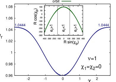
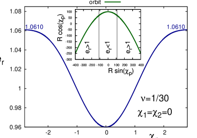
Figure 1: Chameleon orbits due to the 1PN order effects are shown for equal ($\nu=1$, left panel) and asymmetric ($\nu=1/30$, right panel) mass binaries. The chameleon behaviour is characterized by the trespassing of the function $e_{r}\left(\chi_{p}\right)$ across the value 1 (indicated in blue). Initial conditions are fixed at the periastron as $e_{r}\left(\chi_{p}=0\right)=0.96$ and $\varepsilon\left(\chi_{p}=0\right)=Gm/c^{2}r_{\min}=0.01$. The asymptotic values of $e_{r}$ are given (in blue) on the left and right sides on each panel. The orbits $R\cos\chi_{p}$ vs. $R\sin\chi_{p}$ with $R=c^{2}r/Gm$ are shown by the (green) curve in the smaller boxes. The domains with $e_{r}<1$ and $e_{r}>1$, respectively are also indicated.

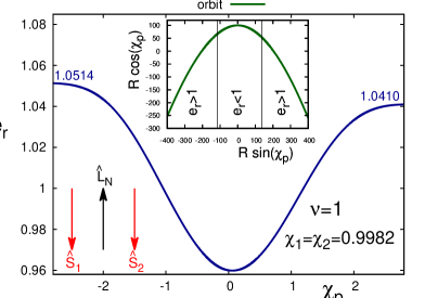
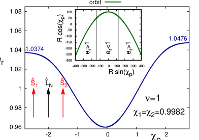
Figure 2: Chameleon orbits due to 1PN and SO effects for binaries with equal masses and spins ($\chi_{1}=\chi_{2}=0.9982$). The curves and initial conditions are as on Fig. 1. On the left (right) panel the spins are anti-aligned (aligned) with the orbital angular momentum.

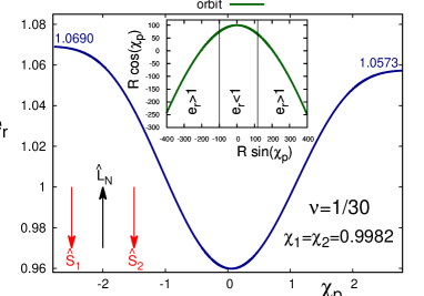
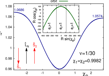
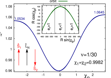
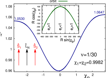
Figure 3: Chameleon orbits created by 1PN and SO effects are represented for unequal mass ($\nu=1/30$) spinning binaries. The same functions as on Fig. 1 are shown for the same initial conditions. The relative direction of the spins and the orbital momentum are indicated by arrows. The dimensionless spin values are the same $\chi_{1}=\chi_{2}=0.9982$ in all panels.

VIII Concluding Remarks

In this paper we have considered the conservative evolution of spinning compact binaries up to the second post-Newtonian order accuracy, by including the leading order spin-orbit, spin-spin and mass quadrupole-monopole contributions. The novel feature of the discussion is that it had been presented in terms of suitably chosen dimensionless variables. These are i) the variables replacing the traditional orbital elements of celestial mechanics: a dimensionless version of the orbital angular momentum, the eccentricity and three Euler angles characterising the orientation of the orbit and the orbital plane with respect to the total angular momentum vector, also ii) dimensionless spin magnitudes (smaller than one for both black holes and neutron stars) together with the spin azimuthal and polar angles. The preferred reference system of this analysis is tied to the orbital angular momentum and periastron.

As a main result we derived a system of first order differential equations in a compact form, for a set of 9 dimensionless variables encompassing both the orbital elements and the spin angles (the spin magnitudes being conserved). These are supplemented by the evolution equation of the true anomaly, which closes the differential system.

These evolutions are constrained by the conservation laws of energy and total angular momentum vector holding at 2PN order. As required by the generic theory of constrained dynamical systems we analyzed the consistency of the constraints, e.g. their compatibility with the evolution equations, and proved that they are preserved by the evolution.

We applied the formalism to show the existence of orbits with unusual features. Close to the periastron, the osculating orbits of these trajectories with eccentricity close to one change from hyperbolic to elliptic, then back to hyperbolic. Hence these orbits (as characterised by the eccentricity of their osculating orbit) look open, then closed, then open again during the passage through the periastron. These chameleon orbits evolve from elliptic (locally, in a Newtonian sense) close to the periastron into hyperbolic (in the same sense) at large distances. Such a property emerges due to the fact that General Relativity predicts stronger gravity (deeper potential wells) at short distances than Newtonian theory does, as also illustrated by the hydrostatic equilibrium in relativistic stars.

We analysed the chameleon orbits as function of mass ratios and spin orientations, for aligned and anti-aligned spin and orbital angular momentum configurations. Without spin, these orbits are symmetric with respect to the periastron. The farther the mass ratio is from unity, the larger is the change in the eccentricity of the osculating orbit, hence the easier to find such chameleon orbits.

The presence of spins can not be detected when the masses are equal and the spins anti-aligned with each other. In all other cases with spin, they induce an asymmetry with respect to the periastron. One aspect of this asymmetry is that the minimum of the eccentricity is not in the periastron, as can be seen on Figs. 2-3. As a rule we found that the alignment of the total spin $\mathbf{S}_{\mathbf{1}}+\mathbf{S}_{2}$ with the orbital angular momentum shifts the minimum eccentricity point of the trajectory before the periastron, while the anti-alignment shifts it after the periastron. These results hold both in the equal mass and in the asymmetric mass cases.

This feature of relativistic orbits is complementary to how the rotation or counterrotation of a particle in circular orbit about a rotating black hole affects the location of the innermost stable orbit. In our case co-rotation apparently speeds up the (reduced mass) particle, while counter-rotation slows it down, after leaving the periastron.

IX Acknowledgements

LÁG was supported by the European Union and the State of Hungary, cofinanced by the European Social Fund in the framework of TÁMOP 4.2.4. A/2-11-/1-2012-0001 ‘National Excellence Program’. ZK has been supported by OTKA Grant No. 100216.

Appendix A Computational details for verifying the 2PN accurate, nonspinning consistency conditions

In this Appendix we give computational details for the proof of the 2PN accurate consistency conditions in the absence of spins.

First we discuss the energy consistency condition (86). After inserting the acceleration components $\mathfrak{a}_{1}^{PN}$, $\mathfrak{a}_{2}^{PN}$, $\mathfrak{a}_{1}^{2PN}$ and $\mathfrak{a}_{2}^{2PN}$, then simplifying with $\sin\chi_{p}$ the coefficients of the 6th order polynomial in $\cos\chi_{p}$, enlisted below, have to vanish.

The terms without $\cos\chi_{p}$ give:

$$0 = \mathrm{s}_{1}e_{r}+16\mathrm{c}_{1\left(0\right)}^{2PN}-16e_{r}\mathrm{c}_{2\left(0\right)}^{2PN}-2\mathrm{c}_{2\left(0\right)}^{PN}\frac{d\mathrm{q}_{0}}{de_{r}}$$ (107)

$$+2\mathrm{c}_{1\left(0\right)}^{PN}\left(2\mathrm{q}_{1}+\frac{d\mathrm{q}_{0}}{de_{r}}e_{r}-4\mathrm{q}_{0}\right)~{},$$

which add up to zero after inserting the definitions of the coefficients $\mathrm{c}_{i(k)}^{PN}$, $\mathrm{c}_{i(k)}^{2PN}$, $\mathrm{q}_{i}$, $\mathrm{s}_{i}$.

The coefficient of $\cos\chi_{p}$ gives:

$$0 = 2\mathrm{s}_{2}e_{r}^{2}+\mathrm{s}_{1}e_{r}^{2}+16\left(\mathrm{c}_{1\left(1\right)}^{2PN}-\mathrm{c}_{2\left(0\right)}^{2PN}\right)$$ (108)

$$+16e_{r}\mathrm{c}_{1\left(0\right)}^{2PN}-16e_{r}\mathrm{c}_{2\left(1\right)}^{2PN}-16\allowbreak e_{r}^{2}\mathrm{c}_{2\left(0\right)}^{2PN}$$

$$-2\mathrm{c}_{2\left(0\right)}^{PN}\left(\frac{d\mathrm{q}_{1}}{de_{r}}+\frac{d\mathrm{q}_{0}}{de_{r}}\right)e_{r}-2\mathrm{c}_{2\left(1\right)}^{PN}\frac{d\mathrm{q}_{0}}{de_{r}}$$

$$+2\left(\mathrm{c}_{1\left(1\right)}^{PN}-\mathrm{c}_{2\left(0\right)}^{PN}\right)\left[2\left(\mathrm{q}_{1}-2\mathrm{q}_{0}\right)+\frac{d\mathrm{q}_{0}}{de_{r}}e_{r}\right]$$

$$+2\mathrm{c}_{1\left(0\right)}^{PN}\left[2\left(2\mathrm{q}_{2}-\mathrm{q}_{1}\right)e_{r}+\frac{d\mathrm{q}_{1}}{de_{r}}e_{r}^{2}+\frac{d\mathrm{q}_{0}}{de_{r}}\right]~{},$$

adding up to zero after inserting the definitions of the coefficients $\mathrm{c}_{i(k)}^{PN}$, $\mathrm{c}_{i(k)}^{2PN}$, $\mathrm{q}_{i}$, $\mathrm{s}_{i}$.

The coefficient of $\cos^{2}\chi_{p}$ gives:

$$0 = 3\mathrm{s}_{3}e_{r}^{3}+2\mathrm{s}_{2}e_{r}^{3}+16\left(\mathrm{c}_{1\left(2\right)}^{2PN}-\mathrm{c}_{2\left(1\right)}^{2PN}\right)$$ (109)

$$-16e_{r}\mathrm{c}_{2\left(2\right)}^{2PN}-16\allowbreak e_{r}^{2}\mathrm{c}_{2\left(1\right)}^{2PN}+16e_{r}\left(\mathrm{c}_{1\left(1\right)}^{2PN}-\mathrm{c}_{2\left(0\right)}^{2PN}\right)$$

$$+2\mathrm{c}_{1\left(0\right)}^{PN}\left(6\mathrm{q}_{3}e_{r}+\frac{d\mathrm{q}_{1}}{de_{r}}\right)e_{r}-2\mathrm{c}_{2\left(2\right)}^{PN}\frac{d\mathrm{q}_{0}}{de_{r}}$$

$$-2\mathrm{c}_{2\left(1\right)}^{PN}\left(\frac{d\mathrm{q}_{1}}{de_{r}}+\frac{d\mathrm{q}_{0}}{de_{r}}\right)e_{r}-2\mathrm{c}_{2\left(0\right)}^{PN}\frac{d\mathrm{q}_{1}}{de_{r}}e_{r}^{2}$$

$$+2\left(\mathrm{c}_{1\left(1\right)}^{PN}-\mathrm{c}_{2\left(0\right)}^{PN}\right)\left[2\left(2\mathrm{q}_{2}-\mathrm{q}_{1}\right)e_{r}+\frac{d\mathrm{q}_{1}}{de_{r}}e_{r}^{2}+\frac{d\mathrm{q}_{0}}{de_{r}}\right]$$

$$+2\left(\mathrm{c}_{1\left(2\right)}^{PN}-\mathrm{c}_{2\left(1\right)}^{PN}\right)\left[2\left(\mathrm{q}_{1}-2\mathrm{q}_{0}\right)+\frac{d\mathrm{q}_{0}}{de_{r}}e_{r}\right]~{},$$

where the terms in the last line cancel by virtue of the relations between the coefficients $\mathrm{c}_{i(k)}^{PN}$, while the first five lines add up to zero after inserting the definitions of the coefficients $\mathrm{c}_{i(k)}^{PN}$, $\mathrm{c}_{i(k)}^{2PN}$, $\mathrm{q}_{i}$, $\mathrm{s}_{i}$.

The coefficient of $\cos^{3}\chi_{p}$ gives:

$$0 = 4\mathrm{s}_{4}e_{r}^{4}+3\mathrm{s}_{3}e_{r}^{4}+16\left(\mathrm{c}_{1\left(3\right)}^{2PN}-\mathrm{c}_{2\left(2\right)}^{2PN}\right)$$ (110)

$$-16e_{r}\mathrm{c}_{2\left(3\right)}^{2PN}-16\allowbreak e_{r}^{2}\mathrm{c}_{2\left(2\right)}^{2PN}+16e_{r}\left(\mathrm{c}_{1\left(2\right)}^{2PN}-\mathrm{c}_{2\left(1\right)}^{2PN}\right)$$

$$-2\mathrm{c}_{2\left(2\right)}^{PN}\left(\frac{d\mathrm{q}_{1}}{de_{r}}+\frac{d\mathrm{q}_{0}}{de_{r}}\right)e_{r}-2\mathrm{c}_{2\left(1\right)}^{PN}\frac{d\mathrm{q}_{1}}{de_{r}}e_{r}^{2}$$

$$+2\left(\mathrm{c}_{1\left(1\right)}^{PN}-\mathrm{c}_{2\left(0\right)}^{PN}\right)\left(6\mathrm{q}_{3}e_{r}+\frac{d\mathrm{q}_{1}}{de_{r}}\right)e_{r}+4\mathrm{c}_{1\left(0\right)}^{PN}\mathrm{q}_{3}e_{r}^{3}$$

$$+2\left(\mathrm{c}_{1\left(2\right)}^{PN}-\mathrm{c}_{2\left(1\right)}^{PN}\right)\left[2\left(2\mathrm{q}_{2}-\mathrm{q}_{1}\right)e_{r}+\frac{d\mathrm{q}_{1}}{de_{r}}e_{r}^{2}+\frac{d\mathrm{q}_{0}}{de_{r}}\right]$$

$$+2\left(\mathrm{c}_{1\left(3\right)}^{PN}-\mathrm{c}_{2\left(2\right)}^{PN}\right)\left[2\left(\mathrm{q}_{1}-2\mathrm{q}_{0}\right)+\frac{d\mathrm{q}_{0}}{de_{r}}e_{r}\right]~{},$$

and the terms in the last two lines cancel by virtue of the relations between the coefficients $\mathrm{c}_{i(k)}^{PN}$, while the first four lines add up to zero after inserting the definitions of the coefficients $\mathrm{c}_{i(k)}^{PN}$, $\mathrm{c}_{i(k)}^{2PN}$, $\mathrm{q}_{i}$, $\mathrm{s}_{i}$.

The coefficient of $\cos^{4}\chi_{p}$ gives:

$$0 = 4\mathrm{s}_{4}e_{r}^{5}-16\allowbreak e_{r}^{2}\mathrm{c}_{2\left(3\right)}^{2PN}+16e_{r}\left(\mathrm{c}_{1\left(3\right)}^{2PN}-\mathrm{c}_{2\left(2\right)}^{2PN}\right)$$ (111)

$$-2\mathrm{c}_{2\left(2\right)}^{PN}\frac{d\mathrm{q}_{1}}{de_{r}}e_{r}^{2}+4\left(\mathrm{c}_{1\left(1\right)}^{PN}-\mathrm{c}_{2\left(0\right)}^{PN}\right)\mathrm{q}_{3}e_{r}^{3}$$

$$+e_{r}\left(5\mathrm{s}_{5}e_{r}^{4}-16\mathrm{c}_{2\left(4\right)}^{2PN}\right)+16\left(\mathrm{c}_{1\left(4\right)}^{2PN}-\mathrm{c}_{2\left(3\right)}^{2PN}\right)$$

$$+2\left(\mathrm{c}_{1\left(3\right)}^{PN}-\mathrm{c}_{2\left(2\right)}^{PN}\right)\left[2\left(2\mathrm{q}_{2}-\mathrm{q}_{1}\right)e_{r}+\frac{d\mathrm{q}_{1}}{de_{r}}e_{r}^{2}+\frac{d\mathrm{q}_{0}}{de_{r}}\right]$$

$$+2\left(\mathrm{c}_{1\left(2\right)}^{PN}-\mathrm{c}_{2\left(1\right)}^{PN}\right)\left(6\mathrm{q}_{3}e_{r}+\frac{d\mathrm{q}_{1}}{de_{r}}\right)e_{r}~{},$$

and the terms in the last three lines cancel by virtue of the relations between the coefficients $\mathrm{c}_{i(k)}^{PN}$, $\mathrm{c}_{i(k)}^{2PN}$, $\mathrm{s}_{i}$, while the first two lines add up to zero after inserting the definitions of the coefficients $\mathrm{c}_{i(k)}^{PN}$, $\mathrm{c}_{i(k)}^{2PN}$, $\mathrm{q}_{i}$, $\mathrm{s}_{i}$.

The coefficient of $\cos^{5}\chi_{p}$ gives:

$$0 = e_{r}^{2}\left(5\mathrm{s}_{5}e_{r}^{4}-16\allowbreak\mathrm{c}_{2\left(4\right)}^{2PN}\right)+16\left(\mathrm{c}_{1\left(5\right)}^{2PN}-\mathrm{c}_{2\left(4\right)}^{2PN}\right)$$ (112)

$$+16e_{r}\left(\mathrm{c}_{1\left(4\right)}^{2PN}-\mathrm{c}_{2\left(3\right)}^{2PN}\right)+4\left(\mathrm{c}_{1\left(2\right)}^{PN}-\mathrm{c}_{2\left(1\right)}^{PN}\right)\mathrm{q}_{3}e_{r}^{3}$$

$$+2\left(\mathrm{c}_{1\left(3\right)}^{PN}-\mathrm{c}_{2\left(2\right)}^{PN}\right)\left(6\mathrm{q}_{3}e_{r}+\frac{d\mathrm{q}_{1}}{de_{r}}\right)e_{r}~{},$$

where all terms cancel by virtue of the relations between the coefficients $\mathrm{c}_{i(k)}^{PN}$, $\mathrm{c}_{i(k)}^{2PN}$, $\mathrm{s}_{i}$.

The coefficient of $\cos^{6}\chi_{p}$ gives:

$$0=4\left(\mathrm{c}_{1\left(5\right)}^{2PN}-\mathrm{c}_{2\left(4\right)}^{2PN}\right)+\left(\mathrm{c}_{1\left(3\right)}^{PN}-\mathrm{c}_{2\left(2\right)}^{PN}\right)\mathrm{q}_{3}e_{r}^{2}~{},$$ (113)

where all terms cancel by virtue of the relations between the coefficients $\mathrm{c}_{i(k)}^{PN}$, $\mathrm{c}_{i(k)}^{2PN}$.

In summary all these 6 equations reduce to identities, confirming the consistency condition arising from energy conservation.

The consistency condition (93), arising from the total angular momentum conservation takes the explicit form $0=\sum_{k=0}^{5}h_{\left(k\right)}\cos\chi_{p}$, with the coefficients

$$h_{\left(0\right)} = \mathrm{b}_{2\left(0\right)}\mathrm{c}_{2\left(0\right)}^{PN}-\mathrm{b}_{1\left(0\right)}\mathrm{c}_{1\left(0\right)}^{PN}-2\mathrm{c}_{1\left(0\right)}^{2PN}-\frac{1}{4}\mathrm{p}_{1}e_{r}$$

$$h_{\left(1\right)} = \mathrm{b}_{2\left(0\right)}\mathrm{c}_{2\left(1\right)}^{PN}-\mathrm{b}_{1\left(0\right)}\mathrm{c}_{1\left(1\right)}^{PN}+\mathrm{b}_{2\left(1\right)}\mathrm{c}_{2\left(0\right)}^{PN}-\mathrm{b}_{1\left(1\right)}\mathrm{c}_{1\left(0\right)}^{PN}$$

$$+2\left(\mathrm{c}_{2\left(0\right)}^{2PN}-\mathrm{c}_{1\left(1\right)}^{2PN}\right)-\left(\frac{1}{2}\mathrm{p}_{2}+\frac{1}{4}\mathrm{p}_{1}\right)e_{r}^{2}$$

$$h_{\left(2\right)} = \mathrm{b}_{2\left(0\right)}\mathrm{c}_{2\left(2\right)}^{PN}-\mathrm{b}_{1\left(0\right)}\mathrm{c}_{1\left(2\right)}^{PN}+\mathrm{b}_{2\left(1\right)}\mathrm{c}_{2\left(1\right)}^{PN}-\mathrm{b}_{1\left(1\right)}\mathrm{c}_{1\left(1\right)}^{PN}$$

$$+\mathrm{b}_{2\left(2\right)}\mathrm{c}_{2\left(0\right)}^{PN}+2\left(\mathrm{c}_{2\left(1\right)}^{2PN}-\mathrm{c}_{1\left(2\right)}^{2PN}\right)\!-\!\!\left(\!\frac{3}{4}\mathrm{p}_{3}\!+\!\frac{1}{2}\mathrm{p}_{2}\!\right)e_{r}^{3}$$

$$h_{\left(3\right)} = \mathrm{b}_{2\left(1\right)}\mathrm{c}_{2\left(2\right)}^{PN}-\mathrm{b}_{1\left(1\right)}\mathrm{c}_{1\left(2\right)}^{PN}-\mathrm{b}_{1\left(0\right)}\mathrm{c}_{1\left(3\right)}^{PN}+\mathrm{b}_{2\left(2\right)}\mathrm{c}_{2\left(1\right)}^{PN}$$

$$+2\left(\mathrm{c}_{2\left(2\right)}^{2PN}-\mathrm{c}_{1\left(3\right)}^{2PN}\right)-\frac{3}{4}\mathrm{p}_{3}e_{r}^{4}$$

$$h_{\left(4\right)} = \mathrm{b}_{2\left(2\right)}\mathrm{c}_{2\left(2\right)}^{PN}-\mathrm{b}_{1\left(1\right)}\mathrm{c}_{1\left(3\right)}^{PN}+2\left(\mathrm{c}_{2\left(3\right)}^{2PN}-\mathrm{c}_{1\left(4\right)}^{2PN}\right)$$

$$h_{\left(5\right)} = 2\left(\mathrm{c}_{2\left(4\right)}^{2PN}-\mathrm{c}_{1\left(5\right)}^{2PN}\right)~{},$$ (114)

all of which vanishing by virtue of the relations between the coefficients $\mathrm{c}_{i(k)}^{PN}$, $\mathrm{c}_{i(k)}^{2PN}$, $\mathrm{b}_{i\left(k\right)}$ and $\mathrm{p}_{i}$. Therefore the consistency condition arising from total angular momentum conservation also holds.

References

- (1) N. Yunes, X. Siemens, Living Rev. Relativity, 16, 9 (2013).
- (2) R. A. Isaacson, Phys. Rev. 166, 1263 (1968); ibid. 166, 1272 (1968).
- (3) L. Blanchet, Living Rev. Relativity 17, 2 (2014).
- (4) E. E. Flanagan, S. A. Hughes, New J. Phys. 7 204 (2005).
- (5) E. Berti, V. Cardoso, A. O. Starinets, Class. Quantum Grav. 26, 163001 (2009).
- (6) A. Buonanno, T. Damour, Phys. Rev. D 59, 084006 (1999), ibid. 62, 064015 (2000); Y. Pan et al., Phys. Rev. D 81, 084041 (2010); A. Taracchini et al., Phys. Rev. D 89, 061502 (2014); Y. Pan et al., Phys. Rev. D 89, 084006 (2014).
- (7) I. Hinder et al., Class. Quantum Grav. 31, 025012 (2014); SXS Gravitational Waveform Database http://www.black-holes.org/waveforms/ .
- (8) The LIGO Collaboration, Phys. Rev. D 80, 047101 (2009); D. Shoemaker (LIGO Collaboration), Advanced LIGO anticipated sensitivity curves, LIGO Document T0900288-v3 (2010).
- (9) K Somiya, Class. Quantum Grav. 29, 124007 (2012).
- (10) The Virgo Collaboration, Advanced Virgo: a 2nd generation interferometric gravitational wave detector, E-print: arXiv:1408.3978 (2014).
- (11) The LIGO Collaboration, The Virgo Collaboration, Class.Quant.Grav. 27, 173001 (2010).
- (12) G. Hobbs et. al., Class. Quantum Grav. 27, 084013 (2010); A. Sesana, A. Vecchio, C. N. Colacino, Mon. Not. Royal Astron. Soc. 390, 192 (2008); A. Sesana, A. Vecchio, M. Volonteri, Mon. Not. Royal Astron. Soc. 394, 2255 (2009).
- (13) K. G. Arun et al., Class. Quantum Grav. 26, 094027 (2009); R. N. Lang, S. A. Hughes, Class. Quantum Grav. 26, 094035 (2009).
- (14) R.-M. Memmesheimer, A. Gopakumar, G. Schäfer, Phys. Rev. D 70, 104011 (2004); P. Ajith et al., Class. Quantum Grav. 24, S689 (2007); A. Buonanno et al., Phys. Rev. D 76, 104049 (2007); Y. Pan et al., Phys. Rev. D 77, 024014 (2008); I. Hinder, F. Herrmann, P. Laguna, D. Shoemaker, Phys. Rev. D 82, 024033 (2010).
- (15) K. Glampedakis, D. Kennefick, Phys. Rev. D 66, 044002 (2002).
- (16) J. Levin, G. Perez-Giz, Phys. Rev. D 77, 103005 (2008); R. Grossman, J. Levin, G. Perez-Giz, Phys. Rev. D 85, 023012 (2012).
- (17) F. Pretorius, D. Khurana, Class. Quantum Grav. 24, S83 (2007); J. Healy, J. Levin, D. Shoemaker, Phys. Rev. Lett. 103, 131101 (2009); U. Sperhake et al., Phys. Rev. Lett. 103, 131102 (2009); R. Gold, B. Bruegmann, Class. Quantum Grav. 27, 084035 (2010).
- (18) R. Gold, B. Bruegmann, Phys. Rev. D 88, 064051 (2013); W. E. East, S. T. McWilliams, J. Levin, F. Pretorius, Phys. Rev. D 87, 043004 (2013).
- (19) J. Levin, R. Grossman, Phys. Rev. D 79, 043016 (2009); R. Grossman, J. Levin, Phys. Rev. D 79, 043017 (2009).
- (20) T. Damour, N. Deruelle, Ann. Inst. Henri Poincaré (Phys. Théor.) 43, 107 (1985).
- (21) B. M. Barker, R. F. O’Connell, Phys. Rev. D 12, 329 (1975); B. M. Barker, R. F. O’Connell, Gen. Relativ. Gravit. 2, 1428 (1979).
- (22) L. E. Kidder, C. M. Will, A. G. Wiseman, Phys. Rev. D 47, R4183 (1993).
- (23) L. E. Kidder, Phys. Rev. D 52, 821 (1995).
- (24) Z. Keresztes, B. Mikóczi, L. Á. Gergely, Phys. Rev. D 72, 104022 (2005). The coefficients in the third line of Table I. and in the first line of Table II. should read as and , respectively; in Eq. (18) the term should have a factor of and the sign of should be switched.
- (25) L. Á. Gergely, Phys. Rev. D 81, 084025 (2010).The power of in Eq. (57) should read
- (26) L. Á. Gergely, Phys. Rev. D 82, 104031 (2010).
- (27) P. C. Peters, J. Matthews, Phys. Rev. 131, 435-440 (1963); P. C. Peters, Phys. Rev. 136, B1224-B1232 (1964).
- (28) T. A. Apostolatos et al., Phys. Rev. D 49, 6274 (1994); F. D. Ryan, Phys. Rev. D 53, 3064 (1996); R. Rieth, G. Schäfer, Class. Quantum Grav. 14, 2357 (1997); L. Á. Gergely, Z. Perjés, M. Vasúth, Phys. Rev. D 57, 876 (1998); ibid. 57, 3423 (1998); ibid. 58, 124001 (1998); R. F. O’Connell, Phys. Rev. Letters 93, 081103 (2004); C. M. Will, Phys. Rev. D 71, 084027 (2005); C. Koenigsdoerffer, A. Gopakumar, Phys. Rev. D 73, 044011 (2006); J. Zeng, C. M. Will, Gen. Rel. Grav. 39 1661-1673 (2007); J. Majár, M. Vasúth, Phys. Rev. D 77, 104005 (2008); N. J. Cornish, J. Shapiro Key, Phys. Rev. D 82, 044028 (2010).
- (29) T. A. Apostolatos, Phys. Rev. D 52, 605 (1995); T. A. Apostolatos, Phys. Rev. D 54, 2438 (1996); B. Mikóczi, M. Vasúth, L. Á. Gergely, Phys. Rev. D 71, 124043 (2005); H. Wang, C. M. Will, Phys. Rev. D 75, 064017 (2007); K. G. Arun et al., Phys. Rev. D 79, 104023 (2009); J. Majár, Phys. Rev. D 80, 104028 (2009); A. Klein, Ph. Jetzer, Phys.Rev. D 81 124001 (2010).
- (30) L. Á. Gergely, Phys. Rev. D 61, 024035 (1999); L. Á. Gergely, Phys. Rev. D 62, 024007 (2000).
- (31) E. Poisson, Phys. Rev. D 57, 5287 (1998).
- (32) L. Á. Gergely, Z. Keresztes, Phys. Rev. D 67, 024020 (2003).
- (33) E. E. Flanagan, T. Hinderer, Phys. Rev. D 75, 124007 (2007); É. Racine, Phys. Rev. D 78, 044021 (2008).
- (34) L. Á. Gergely, P. L. Biermann, Astrophys. J. 697, 1621-1633 (2009); L. Á. Gergely, P. L. Biermann, L. I. Caramete, Class. Quantum Grav. 27, 194009 (2010).
- (35) E. J. Hodges-Kluck et al. Astrophys. J. Lett. 717, L37 (2010); Gopal-Krishna et al., Res. Astron. Astrophys. 12, 127-146 (2012); M. Mezcua et al., Astron. Astrophys. 544, A36 (2012).
- (36) K. S. Thorne, Rev. Mod. Phys. 52, 299 (1980).
- (37) W. G. Laarakkers, E. Poisson, Quadrupole moments of rotating neutron stars. E-print: arXiv:gr-qc/9709033 (1997).
- (38) T. D. Newton, E. P. Wigner, Rev. Mod. Phys. 21, 400 (1949); M. H. L. Pryce, Proc. Roy. Soc. Ser. A 195, 62 (1949).
- (39) M. Vasúth et al., Phys. Rev. D 68, 124006 (2003).
- (40) M. H. Soffel, Relativty in Astrometry, Celestial Mechanics and Geodesy, Springer (1989).
- (41) M. Tápai, Z. Keresztes, L. Á. Gergely, Phys. Rev. D 86, 104045 (2012).
- (42) D. Merritt et al., Phys. Rev. D 81, 062002 (2010).
- (43) M. Turner, Astrophys. J. 216, 610 (1977); S. Capozziello et al., Mod. Phys. Lett. A 23, 99 (2008); S. Capozziello, M. De Laurentis, Astropart. Phys. 30, 105 (2008); J. Majár, P. Forgács, M. Vasúth, Phys. Rev. D 82, 064041 (2010); L. De Vittori, P. Jetzer, A. Klein, Phys. Rev. D 86, 044017 (2012); M. Vasúth, E-print: arXiv:1409.6529 [gr-qc] (2014).
- (44) K. S. Thorne, Astrophys. J. 191, 507 (1974).