Admissible Velocity Propagation : Beyond Quasi-Static Path Planning for High-Dimensional Robots

Abstract

Path-velocity decomposition is an intuitive yet powerful approach to address the complexity of kinodynamic motion planning. The difficult trajectory planning problem is solved in two separate and simpler steps : first, find a path in the configuration space that satisfies the geometric constraints (path planning), and second, find a time-parameterization of that path satisfying the kinodynamic constraints. A fundamental requirement is that the path found in the first step should be time-parameterizable. Most existing works fulfill this requirement by enforcing quasi-static constraints in the path planning step, resulting in an important loss in completeness. We propose a method that enables path-velocity decomposition to discover truly dynamic motions, i.e. motions that are not quasi-statically executable. At the heart of the proposed method is a new algorithm – Admissible Velocity Propagation – which, given a path and an interval of reachable velocities at the beginning of that path, computes exactly and efficiently the interval of all the velocities the system can reach after traversing the path while respecting the system kinodynamic constraints. Combining this algorithm with usual sampling-based planners then gives rise to a family of new trajectory planners that can appropriately handle kinodynamic constraints while retaining the advantages associated with path-velocity decomposition. We demonstrate the efficiency of the proposed method on some difficult kinodynamic planning problems, where, in particular, quasi-static methods are guaranteed to fail .

1 Introduction

Planning motions for robots with many degrees of freedom and subject to kinodynamic constraints (i.e. constraints that involve higher-order time-derivatives of the robot configuration (Donald et al., 1993; LaValle and Kuffner, 2001)) is one of the most important and challenging problems in robotics. Path-velocity decomposition is an intuitive yet powerful approach to address the complexity of kinodynamic motion planning : first, find a path in the configuration space that satisfies the geometric constraints, such as obstacle avoidance, joint limits, kinematic closure, etc. (path planning), and second, find a time-parameterization of that path satisfying the kinodynamic constraints, such as torque limits for manipulators, dynamic balance for legged robots, etc.

Advantages of path-velocity decomposition

This approach was suggested as early as 1986 – only a few years after the birth of motion planning itself as a research field – by Kant and Zucker, in the context of motion planning amongst movable obstacles. Since then, it has become an important tool to address many kinodynamic planning problems, from manipulators subject to torque limits (Bobrow et al., 1985; Shin and McKay, 1986; Bobrow, 1988), to coordination of teams of mobile robots (Siméon et al., 2002; Peng and Akella, 2005), to legged robots subject to balance constraints (Kuffner et al., 2002; Suleiman et al., 2010; Hauser et al., 2008; Escande et al., 2013; Hauser, 2014; Pham and Stasse, 2015), etc. In fact, to our knowledge, path-velocity decomposition [either explicitly or implicitly, as e.g. when only the geometric motion is planned and the time-parameterization is left to the execution phase] is the only motion planning approach that has been shown to work on actual high-DOF robots such as humanoids.

Path-velocity decomposition is appealing in that it exploits the natural decomposition of the constraints, in most systems, into two categories : those depending uniquely on the robot configuration, and those depending in particular on the velocity, which in turn is related to the energy of the system. Consider for instance a humanoid robot in a multi-contact task. Such a robot must (1) avoid collision with the environment, (2) avoid self-collisions, (3) respect kinematic closure for the parts in contact with the environment (e.g. the stance foot must be fixed with respect to the ground), (4) maintain balance. It can be noted that constraints (1 – 3) are exclusively related to the configuration of the robot, while constraint (4), once a path is given, depends mostly on the path velocity.

From a practical viewpoint, the two sub-problems – geometric path planning and kinodynamic time-parameterization – have received so much attention from the robotics community in the past three decades that a large body of theory and good practices exist and can be readily combined to yield efficient trajectory planners. Briefly, high-dimensional and cluttered geometric path planning problems can now be solved in seconds thanks to sampling-based planning algorithms such as PRM (Kavraki et al., 1996) or RRT (Kuffner and LaValle, 2000) and to the dozens of heuristics that have been developed for these algorithms. Regarding kinodynamic time-parameterization, two important discoveries about the structure of the problem have led to particularly efficient algorithmic solutions. First, the bang-bang nature of the optimal velocity profile was identified by (Bobrow et al., 1985; Shin and McKay, 1986), leading to fast numerical integration methods (see Pham, 2014, for extensive historical references). Second, this problem was shown to be reducible to a convex optimization problem, leading to robust and versatile convex-optimization-based solutions (see e.g. Verscheure et al., 2009; Hauser, 2014).

Problems with state-space planning and trajectory optimization approaches

Alternative approaches to path-velocity decomposition include planning directly in the state space and trajectory optimization. The first approach deploys traditional path planners such as RRT (LaValle and Kuffner, 2001) or PRM (Hsu et al., 2002) directly into the state space, that is, the configuration space augmented with velocity coordinates. Three main difficulties are associated with this approach. First, the dimension of the state space is twice that of the configuration space, resulting in higher algorithmic complexity. Second, while connecting two adjacent configurations under geometric constraints is trivial (using e.g. linear segments), connecting two adjacent states under kinodynamic constraints is considerably more challenging and time-consuming, requiring e.g. to solve a two-point boundary value problem (LaValle and Kuffner, 2001) or to sample in the control space and to integrate forward the sampled control (Hsu et al., 2002; Sucan and Kavraki, 2012; Papadopoulos et al., 2014; Li et al., 2015). Third, especially for state-space RRTs, designing a reasonable metric is particularly difficult : Shkolnik et al. (2009) showed that, even for the 1-DOF pendulum subject to torque constraints, a state-space RRT with a simple Euclidean metric is doomed to failure. The authors then proposed to construct an efficient metric by solving local optimal control problems. In a similar fashion, kinodynamic planners based on locally linearized system dynamics were proposed, such as LQR-Tree (Tedrake, 2009) or LQR-RRT^∗ (Perez et al., 2012). While such methods can be applied to low-DOF systems, the necessity to solve an optimal control problem of the dimension of the system at each tree extension makes it unlikely to scale to higher dimensions. For these reasons, in spite of appealing completeness guarantees (under some precise conditions, see e.g. Caron et al., 2014; Papadopoulos et al., 2014; Kunz and Stilman, 2015), there exist, to our knowledge, few examples of successful application of state-space planning to high-DOF systems with complex nonlinear dynamics and constraints in challenging environments (see e.g. Sucan and Kavraki, 2012).

The second approach, trajectory optimization, starts with an initial trajectory, which may not be valid (for example the trajectory may not reach the goal configuration, the robot may collide with the environment or may lose balance at some time instants, etc.) One then iteratively modifies the trajectory so as to decrease a cost – which encodes in particular how much the constraints are violated – until it falls below a certain threshold, implying in turn that the trajectory reaches the goal and all constraints are satisfied. Many interesting variations exist : the iterative modification step may be deterministic (Ratliff et al., 2009) or stochastic (Kalakrishnan et al., 2011), the optimization may be done through contact (Mordatch et al., 2012; Posa and Tedrake, 2013), etc. However, for long time-horizon and high-DOF systems, this approach requires solving a large nonlinear optimization problem, which is computationally challenging because of the huge problem size and the existence of many local minima (see Hauser, 2014, for an extensive discussion of the advantages and limitations of trajectory optimization and comparison with path-velocity decomposition).

The quasi-static condition and its limitations

Coming back to path-velocity decomposition, a fundamental requirement here is that the path found in the first step must be time-parameterizable. A commonly-used method to fulfill this requirement is to consider, in that step, the quasi-static constraints that are derived from the original kinodynamic constraints by assuming that the motion is executed at zero velocity. Indeed, the so-derived quasi-static constraints can be expressed using only configuration-space variables, in such a way that planning with quasi-static constraints is purely a geometric path planning problem. In the context of legged robots for example, the balance of the robot at zero velocity is guaranteed when the projection of the center of gravity lies in the support area – a purely geometric condition. This quasi-static condition is assumed in most works dedicated to the planning of complex humanoid motions (see e.g. Kuffner et al., 2002).

This workaround suffers however from a major limitation : the quasi-static condition may be too restrictive and one thus may overlook many possible solutions, i.e. incurring an important loss in completeness. For instance, legged robots walking with ZMP-based control (Vukobratovic et al., 2001) are dynamically balanced but almost never satisfy the aforementioned quasi-static condition on the center of gravity. Another example is provided by an actuated pendulum subject to severe torque limits, but which can still be put into the upright position by swinging back and forth several times. It is clear that such solutions make an essential use of the system dynamics and can in no way be discovered by quasi-static methods, nor by any method that considers only configuration-space coordinates.

Planning truly dynamic motions

Here we propose a method to overcome this limitation. At the heart of the proposed method is a new algorithm – Admissible Velocity Propagation (AVP) – which is based in turn on the classical Time-Optimal Path Parameterization (TOPP) algorithm first introduced by Bobrow et al. (1985); Shin and McKay (1986) and later perfected by many others (see Pham, 2014, and references therein). In contrast with TOPP, which determines one optimal velocity profile along a given path, AVP addresses all valid velocity profiles along that path, requiring only slightly more computation time than TOPP itself. Combining AVP with usual sampling-based path planners, such as RRT, gives rise to a family of new trajectory planners that can appropriately handle kinodynamic constraints while retaining the advantages associated with path-velocity decomposition.

The remainder of this article is organized as follows. In Section 2, we briefly recall the fundamentals of TOPP before presenting AVP. In Section 3, we show how to combine AVP with usual sampling-based path planners such as RRT. In Section 4, we demonstrate the efficiency of the new AVP-based planners on some challenging kinodynamic planning problems – in particular, those where the quasi-static approach is guaranteed to fail. In one of the applications, the planned motion is executed on an actual 6-DOF robot. Finally, in Section 5, we discuss the advantages and limitations of the proposed approach (one particular limitation is that the approach does not a priori apply to under-actuated systems) and sketch some future research directions.

2 Propagating admissible velocities along a path

2.1 Background : Time-Optimal Path Parameterization (TOPP)

As mentioned in the Introduction, there are two main approaches to TOPP : “numerical integration” and “convex optimization”. We briefly recall the numerical integration approach (Bobrow et al., 1985; Shin and McKay, 1986), on which AVP is based. For more details about this approach, the reader is referred to Pham (2014).

Let $\mathbf{q}$ be an $n$-dimensional vector representing the configuration of a robot system. Consider second-order inequality constraints of the form (Pham, 2014)

$$\mathbf{A}(\mathbf{q})\ddot{\mathbf{q}}+\dot{\mathbf{q}}^{\top}\mathbf{B}(\mathbf{q})\dot{\mathbf{q}}+\mathbf{f}(\mathbf{q})\leq 0,$$ (1)

where $\mathbf{A}(\mathbf{q})$, $\mathbf{B}(\mathbf{q})$ and $\mathbf{f}(\mathbf{q})$ are respectively an $M\times n$ matrix, an $n\times M\times n$ tensor and an $M$-dimensional vector. Inequality (1) is general and may represent a large variety of second-order systems and constraints, such as fully-actuated manipulators  subject to velocity, acceleration or torque limits (see e.g. Bobrow et al., 1985; Shin and McKay, 1986), wheeled vehicles subject to sliding and tip-over constraints (Shiller and Gwo, 1991), etc. Redundantly-actuated systems, such as closed-chain manipulators subject to torque limits or legged robots in multi-contact subject to stability constraints, can also be represented by inequality (1) (Pham and Stasse, 2015). However, under-actuated systems cannot be in general taken into account by the framework, see Section 5 for a more detailed discussion.

Note that “direct” velocity bounds of the form

$$\dot{\mathbf{q}}^{\top}\mathbf{B}_{v}(\mathbf{q})\dot{\mathbf{q}}+\mathbf{f}_{v}(\mathbf{q})\leq 0,$$ (2)

can also be taken into account (Zlajpah, 1996). For clarity, we shall not include such “direct” velocity bounds in the following development. Rather, we shall discuss separately how to deal with such bounds in Section 2.3.

Consider now a path $\mathcal{P}$ in the configuration space, represented as the underlying path of a trajectory $\mathbf{q}(s)_{s\in[0,s_{\mathrm{end}}]}$. Assume that $\mathbf{q}(s)_{s\in[0,s_{\mathrm{end}}]}$ is $C^{1}$- and piecewise $C^{2}$-continuous.

Definition 1

A time-parameterization of $\mathcal{P}$ – or time-reparameterization of $\mathbf{q}(s)_{s\in[0,s_{\mathrm{end}}]}$ – is an increasing scalar function $s:[0,T^{\prime}]\rightarrow[0,s_{\mathrm{end}}]$. A time-parameterization can be seen alternatively as a velocity profile, which is the curve $\dot{s}(s)_{s\in[0,s_{\mathrm{end}}]}$ in the $s$–$\dot{s}$ plane. We say that a time-parameterization or, equivalently, a velocity profile, is valid if $s(t)_{t\in[0,T^{\prime}]}$ is continuous, $\dot{s}$ is always strictly positive, and the retimed trajectory $\mathbf{q}(s(t))_{t\in[0,T^{\prime}]}$ satisfies the constraints of the system.

To check whether the retimed trajectory satisfies the system constraints, one may differentiate $\mathbf{q}(s(t))$ with respect to $t$ :

$$\dot{\mathbf{q}}=\mathbf{q}_{s}\dot{s},\quad\ddot{\mathbf{q}}=\mathbf{q}_{s}\ddot{s}+\mathbf{q}_{ss}\dot{s}^{2},$$ (3)

where dots denote differentiations with respect to the time parameter $t$ and $\mathbf{q}_{s}=\frac{\mathrm{d}\mathbf{q}}{\mathrm{d}s}$ and $\mathbf{q}_{ss}=\frac{\mathrm{d}^{2}\mathbf{q}}{\mathrm{d}s^{2}}$. Substituting (3) into (1) then leads to

$$\ddot{s}\mathbf{A}(\mathbf{q})\mathbf{q}_{s}+\dot{s}^{2}\mathbf{A}(\mathbf{q})\mathbf{q}_{ss}+\dot{s}^{2}\mathbf{q}_{s}^{\top}\mathbf{B}(\mathbf{q})\mathbf{q}_{s}+\mathbf{f}(\mathbf{q})\leq 0,$$

which can be rewritten as

$$\ddot{s}\mathbf{a}(s)+\dot{s}^{2}\mathbf{b}(s)+\mathbf{c}(s)\leq 0,\quad\textrm{where}$$ (4)

$$\mathbf{a}(s) \stackrel{{\scriptstyle\mathrm{def}}}{{=}} \mathbf{A}(\mathbf{q}(s))\mathbf{q}_{s}(s),$$

$$\mathbf{b}(s) \stackrel{{\scriptstyle\mathrm{def}}}{{=}} \mathbf{A}(\mathbf{q}(s))\mathbf{q}_{ss}(s)+\mathbf{q}_{s}(s)^{\top}\mathbf{B}(\mathbf{q}(s))\mathbf{q}_{s}(s),$$ (5)

$$\mathbf{c}(s) \stackrel{{\scriptstyle\mathrm{def}}}{{=}} \mathbf{f}(\mathbf{q}(s)).$$

Each row $i$ of equation (4) is of the form

$$a_{i}(s)\ddot{s}+b_{i}(s)\dot{s}^{2}+c_{i}(s)\leq 0.$$

Next,

• if $a_{i}(s)>0$, then one has $\ddot{s}\leq\frac{-c_{i}(s)-b_{i}(s)\dot{s}^{2}}{a_{i}(s)}$. Define the acceleration upper bound $\beta_{i}(s,\dot{s})\stackrel{{\scriptstyle\mathrm{def}}}{{=}}\frac{-c_{i}(s)-b_{i}(s)\dot{s}^{2}}{a_{i}(s)}$;

• if $a_{i}(s)<0$, then one has $\ddot{s}\geq\frac{-c_{i}(s)-b_{i}(s)\dot{s}^{2}}{a_{i}(s)}$. Define the acceleration lower bound $\alpha_{i}(s,\dot{s})\stackrel{{\scriptstyle\mathrm{def}}}{{=}}\frac{-c_{i}(s)-b_{i}(s)\dot{s}^{2}}{a_{i}(s)}$.

One can then define for each $(s,\dot{s})$

$$\alpha(s,\dot{s})\stackrel{{\scriptstyle\mathrm{def}}}{{=}}\max_{i}\alpha_{i}(s,\dot{s}),\quad\beta(s,\dot{s})\stackrel{{\scriptstyle\mathrm{def}}}{{=}}\min_{i}\beta_{i}(s,\dot{s}).$$

From the above transformations, one can conclude that $\mathbf{q}(s(t))_{t\in[0,T^{\prime}]}$ satisfies the constraints (1) if and only if

$$\forall t\in[0,T^{\prime}]\quad\alpha(s(t),\dot{s}(t))\leq\ddot{s}(t)\leq\beta(s(t),\dot{s}(t)).$$ (6)

Note that $(s,\dot{s})\mapsto(\dot{s},\alpha(s,\dot{s}))$ and $(s,\dot{s})\mapsto(\dot{s},\beta(s,\dot{s}))$ can be viewed as two vector fields in the $s$–$\dot{s}$ plane. One can integrate velocity profiles following the field $(\dot{s},\alpha(s,\dot{s}))$ (from now on, $\alpha$ in short) to obtain minimum acceleration profiles (or $\alpha$-profiles), or following the field $\beta$ to obtain maximum acceleration profiles (or $\beta$-profiles).

Next, observe that if $\alpha(s,\dot{s})>\beta(s,\dot{s})$ then, from (6), there is no possible value for $\ddot{s}$. Thus, to be valid, every velocity profile must stay below the maximum velocity curve ($\mathrm{MVC}$ in short) defined by 

$$\mathrm{MVC}(s)\stackrel{{\scriptstyle\mathrm{def}}}{{=}}\left\{\begin{array}[]{cl}\min\{\dot{s}\geq 0:\alpha(s,\dot{s})=\beta(s,\dot{s})\}&\mathrm{if}\ \alpha(s,0)\leq\beta(s,0),\\ 0&\mathrm{if}\ \alpha(s,0)>\beta(s,0).\end{array}\right.$$ (7)

It was shown (see e.g. Shiller and Lu, 1992) that the time-minimal velocity profile is obtained by a bang-bang-type control, i.e., whereby the optimal profile follows alternatively the $\beta$ and $\alpha$ fields while always staying below the $\mathrm{MVC}$. A method to find the optimal profile then consists in (see Fig. 1A for illustration) :

• find all the possible $\alpha\rightarrow\beta$ switch points. There are three types of such switch points : “discontinuous”, “singular” or “tangent” and they must all be on the $\mathrm{MVC}$. The procedure to find these switch points is detailed in Pham (2014);

• from each of these switch points, integrate backward following $\alpha$ and forward following $\beta$ to obtain the Limiting Curves ($\mathrm{LC}$) (Slotine and Yang, 1989);

• construct the Concatenated Limiting Curve (CLC) by considering, for each $s$, the value of the lowest $\mathrm{LC}$ at $s$;

• integrate forward from $(0,\dot{s}_{\mathrm{beg}})$ following $\beta$ and backward from $(s_{\mathrm{end}},\dot{s}_{\mathrm{end}})$ following $\alpha$, and consider the intersection of these profiles with each other or with the CLC. Note that the path velocities $\dot{s}_{\mathrm{beg}}$ and $\dot{s}_{\mathrm{end}}$ are computed from the desired initial and final velocities $v_{\mathrm{beg}}$ and $v_{\mathrm{end}}$ by

  $$\dot{s}_{\mathrm{beg}}\stackrel{{\scriptstyle\mathrm{def}}}{{=}}v_{\mathrm{beg}}/\|\mathbf{q}_{s}(0)\|,\quad\dot{s}_{\mathrm{end}}\stackrel{{\scriptstyle\mathrm{def}}}{{=}}v_{\mathrm{end}}/\|\mathbf{q}_{s}(s_{\mathrm{end}})\|.$$ (8)

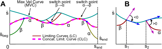
Figure 1: A : Illustration for Maximum Velocity Curve (MVC) and Concatenated Limiting Curve (CLC). The optimal velocity profile follows the green $\beta$-profile, then a portion of the CLC, and finally the yellow $\alpha$-profile. B : Illustration for the Switch Point Lemma.

We now prove two lemmata that will be important later on.

Lemma 1 (Switch Point Lemma)

Assume that a forward $\beta$-profile hits the $\mathrm{MVC}$ at $s=s_{1}$ and a backward $\alpha$-profile hits the $\mathrm{MVC}$ at $s=s_{2}$, with $s_{1}<s_{2}$, then there exists at least one $\alpha\rightarrow\beta$ switch point on the $\mathrm{MVC}$ at some position $s_{3}\in[s_{1},s_{2}]$.

Proof At $(s_{1},\mathrm{MVC}(s_{1}))$, the angle from the vector $\beta$ to the tangent to the $\mathrm{MVC}$ is negative (see Fig. 1B). In addition, since we are on the $\mathrm{MVC}$, we have $\alpha=\beta$, thus the angle from $\alpha$ to the tangent is negative too. Next, at $(s_{2},\mathrm{MVC}(s_{2}))$, the angle of $\alpha$ to the tangent to the $\mathrm{MVC}$ is positive (see Fig. 1B). Thus, since the vector field $\alpha$ is continuous, there exists, between $s_{1}$ and $s_{2}$

1. either a point where the angle between $\alpha$ and the tangent to the $\mathrm{MVC}$ is 0 – in which case we have a tangent switch point;

2. or a point where the $\mathrm{MVC}$ is discontinuous – in which case we have a discontinuous switch point;

3. or a point where the $\mathrm{MVC}$ is continuous but non differentiable – in which case we have a singular switch point.

For more details, the reader is referred to Pham (2014). $\Box$

Lemma 2 (Continuity of the CLC)

Either one of the $\mathrm{LC}$’s reaches $\dot{s}=0$, or the $\mathrm{CLC}$ is continuous.

Proof Assume by contradiction that no $\mathrm{LC}$ reaches $\dot{s}=0$ and that there exists a “hole” in the $\mathrm{CLC}$. The left border $s_{1}$ of the hole must then be defined by the intersection of the $\mathrm{MVC}$ with a forward $\beta$-$\mathrm{LC}$ (coming from the previous $\alpha\rightarrow\beta$ switch point), and the right border $s_{2}$ of the hole must be defined by the intersection of the $\mathrm{MVC}$ with a backward $\alpha$-$\mathrm{LC}$ (coming from the following $\alpha\rightarrow\beta$ switch point). By Lemma 1 above, there must then exist a switch point between $s_{1}$ and $s_{2}$, which contradicts the definition of the hole. $\Box$

2.2 Admissible Velocity Propagation (AVP)

This section presents the Admissible Velocity Propagation algorithm (AVP), which constitutes the heart of our approach. This algorithm takes as inputs :

• a path $\mathcal{P}$ in the configuration space, and

• an interval $[\dot{s}_{\mathrm{beg}}^{\min},\dot{s}_{\mathrm{beg}}^{\max}]$ of initial path velocities;

and returns the interval (cf. Theorem 1) $[\dot{s}_{\mathrm{end}}^{\min},\dot{s}_{\mathrm{end}}^{\max}]$ of all path velocities that the system can reach at the end of $\mathcal{P}$ after traversing $\mathcal{P}$ while respecting the system constraints . The algorithm comprises the following three steps :

A

Compute the limiting curves;

B

Determine the maximum final velocity $\dot{s}_{\mathrm{end}}^{\max}$ by integrating forward from $s=0$;

C

Determine the minimum final velocity $\dot{s}_{\mathrm{end}}^{\min}$ by bisection search and by integrating backward from $s=s_{\mathrm{end}}$.

We now detail each of these steps.

A   Computing the limiting curves

We first compute the Concatenated Limiting Curve (CLC) as shown in Section 2.1. From Lemma 2, either one of the $\mathrm{LC}$’s reaches 0 or the $\mathrm{CLC}$ is continuous. The former case is covered by A1 below, while the latter is covered by A2–5.

A1

One of the $\mathrm{LC}$’s hits the line $\dot{s}=0$. In this case, the path cannot be traversed by the system without violating the kinodynamic constraints : AVP returns Failure. Indeed, assume that a backward ($\alpha$) profile hits $\dot{s}=0$. Then any profile that goes from $s=0$ to $s=s_{\mathrm{end}}$ must cross that profile somewhere and from above, which violates the $\alpha$ bound (see Figure 2A). Similarly, if a forward ($\beta$) profile hits $\dot{s}=0$, then that profile must be crossed somewhere and from below, which violates the $\beta$ bound. Thus, no valid profile can go from $s=0$ to $s=s_{\mathrm{end}}$;

A                                           B

Figure 2: Illustration for step A (computation of the $\mathrm{LC}$’s). A : illustration for case A1. A profile that crosses an $\alpha$-$\mathrm{CLC}$ violates the $\alpha$ bound. B : illustration for case A3.

The CLC is now assumed to be continuous and strictly positive. Since it is bounded by $s=0$ from the left, $s=s_{\mathrm{end}}$ from the right, $\dot{s}=0$ from the bottom and the MVC from the top, there are only four exclusive and exhaustive cases, listed below.

A2

The $\mathrm{CLC}$ hits the $\mathrm{MVC}$ while integrating backward and while integrating forward. In this case, let $\dot{s}_{\mathrm{beg}}^{*}\stackrel{{\scriptstyle\mathrm{def}}}{{=}}\mathrm{MVC}(0)$ and go to B. The situation where there is no switch point is assimilated to this case;

A3

The $\mathrm{CLC}$ hits $s=0$ while integrating backward, and the $\mathrm{MVC}$ while integrating forward (see Figure 2B). In this case, let $\dot{s}_{\mathrm{beg}}^{*}\stackrel{{\scriptstyle\mathrm{def}}}{{=}}\mathrm{CLC}(0)$ and go to B;

A4

The $\mathrm{CLC}$ hits the $\mathrm{MVC}$ while integrating backward, and $s=s_{\mathrm{end}}$ while integrating forward. In this case, let $\dot{s}_{\mathrm{beg}}^{*}\stackrel{{\scriptstyle\mathrm{def}}}{{=}}\mathrm{MVC}(0)$ and go to B;

A5

The $\mathrm{CLC}$ hits $s=0$ while integrating backward, and $s=s_{\mathrm{end}}$ while integrating forward. In this case, let $\dot{s}_{\mathrm{beg}}^{*}\stackrel{{\scriptstyle\mathrm{def}}}{{=}}\mathrm{CLC}(0)$ and go to B.

B   Determining the maximum final velocity

Note that, in any of the cases A2–5, $\dot{s}_{\mathrm{beg}}^{*}$ was defined so that no valid profile can start above it. Thus, if $\dot{s}_{\mathrm{beg}}^{\min}>\dot{s}_{\mathrm{beg}}^{*}$, the path is not traversable : AVP returns Failure. Otherwise, the interval of valid initial velocities is $[\dot{s}_{\mathrm{beg}}^{\min},\dot{s}_{\mathrm{beg}}^{{\max}*}]$ where $\dot{s}_{\mathrm{beg}}^{{\max}*}\stackrel{{\scriptstyle\mathrm{def}}}{{=}}\min(\dot{s}_{\mathrm{beg}}^{\max},\dot{s}_{\mathrm{beg}}^{*})$.

Definition 2

Under the nomenclature introduced in Definition 1, we say that a velocity $\dot{s}_{\mathrm{end}}$ is a valid final velocity if there exists a valid profile that starts at $(0,\dot{s}_{0})$ for some $\dot{s}_{0}\in[\dot{s}_{\mathrm{beg}}^{\min},\dot{s}_{\mathrm{beg}}^{\max}]$ and ends at $(s_{\mathrm{end}},\dot{s}_{\mathrm{end}})$.

We argue that the maximum valid final velocity can be obtained by integrating forward from $\dot{s}_{\mathrm{beg}}^{{\max}*}$ following $\beta$. Let’s call $\Phi$ the velocity profile obtained by doing so. Since $\Phi$ is continuous and bounded by $s=s_{\mathrm{end}}$ from the right, $\dot{s}=0$ from the bottom, and either the MVC or the CLC from the top, there are four exclusive and exhaustive cases, listed below (see Figure 3 for illustration).

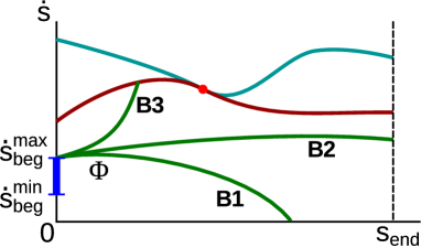
Figure 3: Illustration for step B : one can determine the maximum final velocity by integrating forward from $(0,\dot{s}_{\mathrm{beg}}^{*})$.

B1

$\Phi$ hits $\dot{s}=0$ (cf. profile B1 in Fig. 3). Here, as in the case A1, the path is not traversable : AVP returns Failure. Indeed, any profile that starts below $\dot{s}_{\mathrm{beg}}^{{\max}*}$ and tries to reach $s=s_{\mathrm{end}}$ must cross $\Phi$ somewhere and from below, thus violating the $\beta$ bound;

B2

$\Phi$ hits $s=s_{\mathrm{end}}$ (cf. profile B1 in Fig. 3). Then $\Phi(s_{\mathrm{end}})$ corresponds to the $\dot{s}_{\mathrm{end}}^{\max}$ we are looking for. Indeed, $\Phi(s_{\mathrm{end}})$ is reachable – precisely by $\Phi$ –, and to reach any value above $\Phi(s_{\mathrm{end}})$, the corresponding profile would have to cross $\Phi$ somewhere and from below;

B3

$\Phi$ hits the $\mathrm{CLC}$. There are two sub-cases:

1. If we proceed from cases A4 or A5 (in which the $\mathrm{CLC}$ reaches $s=s_{\mathrm{end}}$, cf. profile B3 in Fig. 3), then $\mathrm{CLC}(s_{\mathrm{end}})$ corresponds to the $\dot{s}_{\mathrm{end}}^{\max}$ we are looking for. Indeed, $\mathrm{CLC}(s_{\mathrm{end}})$ is reachable – precisely by the concatenation of $\Phi$ and the $\mathrm{CLC}$ –, and no value above $\mathrm{CLC}(s_{\mathrm{end}})$ can be valid by the definition of the $\mathrm{CLC}$;

2. If we proceed from cases A2 or A3, then the $\mathrm{CLC}$ hits the $\mathrm{MVC}$ while integrating forward, say at $s=s_{1}$; we then proceed as in case B4 below;

B4

$\Phi$ hits the $\mathrm{MVC}$, say at $s=s_{1}$. It is clear that $\mathrm{MVC}(s_{\mathrm{end}})$ is an upper bound of the valid final velocities, but we have to ascertain whether this value is reachable. For this, we use the predicate IS_VALID defined in Box 1 of C :

• if IS_VALID$(\mathrm{MVC}(s_{\mathrm{end}}))$, then $\mathrm{MVC}(s_{\mathrm{end}})$ is the $\dot{s}_{\mathrm{end}}^{\max}$ we are looking for;

• else, the path is not traversable : AVP returns Failure. Indeed, as we shall see, if for a certain $\dot{s}_{\mathrm{test}}$, the predicate IS_VALID($\dot{s}_{\mathrm{test}}$) is False, then no velocity below $\dot{s}_{\mathrm{test}}$ can be valid either.

C   Determining the minimum final velocity

Assume that we proceed from the cases B2–4. Consider a final velocity $\dot{s}_{\mathrm{test}}$ where

• $\dot{s}_{\mathrm{test}}<\Phi(s_{\mathrm{end}})$ if we proceed from B2;

• $\dot{s}_{\mathrm{test}}<\mathrm{CLC}(s_{\mathrm{end}})$ if we proceed from B3a;

• $\dot{s}_{\mathrm{test}}<\mathrm{MVC}(s_{\mathrm{end}})$ if we proceed from B3b or B4.

Let us integrate backward from $(s_{\mathrm{end}},\dot{s}_{\mathrm{test}})$ following $\alpha$ and call the resulting profile $\Psi$. We have the following lemma.

Lemma 3

$\Psi$ cannot hit the $\mathrm{MVC}$ before hitting either $\Phi$ or the $\mathrm{CLC}$.

Proof If we proceed from B2 or B3a, then it is clear that $\Psi$ must first hit $\Phi$ (case B2) or the $\mathrm{CLC}$ (case B3a) before hitting the $\mathrm{MVC}$. If we proceed from B3b or B4, assume by contradiction that $\Psi$ hits the $\mathrm{MVC}$ first at a position $s=s_{2}$. Then by Lemma 1, there must exist a switch point between $s_{2}$ and the end of the $\mathrm{CLC}$ (in case B3b) or the end of $\Phi$ (in case B4). In both cases, there is a contradiction with the fact that the $\mathrm{CLC}$ is continuous. $\Box$

We can now detail in Box 1 the predicate IS_VALID which assesses whether a final velocity $\dot{s}_{\mathrm{test}}$ is valid.

Input: candidate final velocity $\dot{s}_{\mathrm{test}}$

Output: True iff there exists a valid velocity profile with final velocity $\dot{s}_{\mathrm{test}}$

Consider the profile $\Psi$ constructed above. Since it must hit $\Phi$ or the CLC before hitting the MVC, the following five cases are exclusive and exhaustive (see Fig. 4 for illustrations) :

C1

$\Psi$ hits $\dot{s}=0$ (Fig. 4, profile C1). Then, as in cases A1 or B1, no velocity profile can reach $s_{\mathrm{test}}$ : return False;

C2

$\Psi$ hits $s=0$ for some $\dot{s}_{0}<\dot{s}_{\mathrm{beg}}^{\min}$ (see Figure 4, profile C2). Then any profile that ends at $\dot{s}_{\mathrm{test}}$ would have to hit $\Psi$ from above, which is impossible : return False;

C3

$\Psi$ hits $s=0$ at a point $\dot{s}_{0}\in[\dot{s}_{\mathrm{beg}}^{\min},\dot{s}_{\mathrm{beg}}^{{\max}*}]$ (Fig. 4, profile C3). Then $\dot{s}_{\mathrm{test}}$ can be reached following the valid velocity profile $\Psi$ : return True. (Note that, if $\dot{s}_{0}>\dot{s}_{\mathrm{beg}}^{{\max}*}$ then $\Psi$ must have crossed $\Phi$ somewhere before arriving at $s=0$, which is covered by case C4 below);

C4

$\Psi$ hits $\Phi$ (Fig. 4, profile C4). Then $\dot{s}_{\mathrm{test}}$ can be reached, precisely by the concatenation of a part of $\Phi$ and $\Psi$ : return True;

C5

$\Psi$ hits the $\mathrm{CLC}$ (Fig. 4, profile C5). Then $\dot{s}_{\mathrm{test}}$ can be reached, precisely by the concatenation of $\Phi$, a part of the $\mathrm{CLC}$ and $\Psi$ : return True.

Box 1 IS_VALID

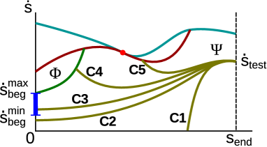
Figure 4: Illustration for the predicate IS_VALID : one can assess whether a final velocity $\dot{s}_{\mathrm{test}}$ is valid by integrating backward from $(s_{\mathrm{end}},\dot{s}_{\mathrm{test}})$.

At this point, we have that, either the path is not traversable, or we have determined $\dot{s}_{\mathrm{end}}^{\max}$ in B. Remark from C3–5 that, if some $\dot{s}_{0}$ is a valid final velocity, then any $\dot{s}\in[\dot{s}_{0},\dot{s}_{\mathrm{end}}^{\max}]$ is also valid. Similarly, from C1 and C2, if some $\dot{s}_{0}$ is not a valid final velocity, then no $\dot{s}\leq s_{0}$ can be valid. We have thus established the following result :

Theorem 1

The set of valid final velocities is an interval.

This interval property enables one to efficiently search for the minimum final velocity as follows. First, test whether $0$ is a valid final velocity: if IS_VALID$(0)$, then the sought-after $\dot{s}_{\mathrm{end}}^{\min}$ is 0. Else, run a standard bisection search with initial bounds $(0,\dot{s}_{\mathrm{end}}^{\max}]$ where 0 is not valid and $\dot{s}_{\mathrm{end}}^{\max}$ is valid. Thus, after executing $\log_{2}(1/\epsilon)$ times the routine IS_VALID, one can determine $\dot{s}_{\mathrm{end}}^{\min}$ with a precision $\epsilon$.

2.3 Remarks

Implementation and complexity of AVP

As clear from the previous section, AVP can be readily adapted from the numerical integration approach to TOPP. As a matter of fact, we implemented AVP in about 100 lines of C++ code based on the TOPP library we developed previously (see https://github.com/quangounet/TOPP).

In terms of complexity, the main difference between AVP and TOPP lies in the bisection search of step C, which requires $\log(1/\epsilon)$ backward integrations. However, in practice, these integrations terminate quickly, either by hitting the MVC or the line $\dot{s}=0$. Thus, the actual running time of AVP is only slightly larger than that of TOPP. As illustration, in the bottle experiment of Section 4.2, we considered 100 random paths, discretized with grid size $N=1000$. TOPP and AVP (with the bisection precision $\epsilon=0.01$) under velocity, acceleration and balance constraints took the same amount of computation time 0.033 $\pm$ 0.003 s per path.

“Direct” velocity bounds

“Direct” velocity bounds in the form of (2) give rise to another maximum velocity curve, say $\mathrm{MVC}_{D}$, in the $(s,\dot{s})$ space. When a forward profile intersects $\mathrm{MVC}_{D}$ (before reaching the “Bobrow’s $\mathrm{MVC}$”), several cases can happen :

1. If “sliding” along the $\mathrm{MVC}_{D}$ does not violate the actuation bounds (1), then slide as far as possible along the $\mathrm{MVC}$. The “slide” terminates either (a) when the maximum acceleration vector $\beta$ points downward from the $\mathrm{MVC}_{D}$: in this case follow that vector out of $\mathrm{MVC}_{D}$ or (b) when the minimum acceleration vector $\alpha$ points upward from the $\mathrm{MVC}_{D}$: in this case, proceed as in 2;

2. If not, then search forward on the $\mathrm{MVC}_{D}$ until finding a point from which one can integrate backward. Such a point is guaranteed to exist and the backward profile will intersect the forward profile.

For more details, the reader is referred to (Zlajpah, 1996).

This reasoning can be extended to AVP: when integrating the forward or the backward profiles (in steps A, B, C of the algorithm), each time a profile intersects the $\mathrm{MVC}_{D}$, one simply applies the above steps.

AVP-backward

Consider the “AVP-backward” problem : given an interval of final velocities $[\dot{s}_{\mathrm{end}}^{\min},\dot{s}_{\mathrm{end}}^{\max}]$, compute the interval $[\dot{s}_{\mathrm{beg}}^{\min},\dot{s}_{\mathrm{beg}}^{\max}]$ of all possible initial velocities. As we shall see in Section 3.2, AVP-backward is essential for the bi-directional version of AVP-RRT (see also Nakamura and Mukherjee, 1991).

It turns out that AVP-backward can be easily obtained by modifying AVP as follows (Lertkultanon and Pham, 2014) :

• step A of AVP-backward is the same as in AVP;

• in step B of AVP-backward, one integrates backward from $\dot{s}_{\mathrm{end}}^{{\min}*}$ instead of integrating forward from $\dot{s}_{\mathrm{beg}}^{{\max}*}$;

• in the bisection search of step C of AVP-backward, one integrates forward from $(0,\dot{s}_{\mathrm{test}})$ instead of integrating backward from$(s_{\mathrm{end}},\dot{s}_{\mathrm{test}})$.

Convex optimization approach

As mentioned in the Introduction, “convex optimization” is another possible approach to TOPP (Verscheure et al., 2009; Hauser, 2014). It is however unclear to us whether one can modify that approach to yield a “convex-optimization-based AVP” other than sampling a large number of $(\dot{s}_{\mathrm{start}},\dot{s}_{\mathrm{end}})$ pairs and running the “convex-optimization-based TOPP” between $(0,\dot{s}_{\mathrm{start}})$ and $(s_{\mathrm{end}},\dot{s}_{\mathrm{end}})$, which would arguably be very slow.

3 Kinodynamic trajectory planning using AVP

3.1 Combining AVP with sampling-based planners

The AVP algorithm presented in Section 2.2 is general and can be combined with various iterative path planners. As an example, we detail in Box 2 and illustrate in Figure 5 a planner we call AVP-RRT, which results from the combination of AVP with the standard RRT path planner (Kuffner and LaValle, 2000).

As in the standard RRT, AVP-RRT iteratively constructs a tree $\mathcal{T}$ in the configuration space. However, in contrast with the standard RRT, a vertex $V$ here consists of a triplet ($V$.config, $V$.inpath, $V$.interval) where $V$.config is an element of the configuration space $\mathscr{C}$, $V$.inpath is a path $\mathcal{P}\subset\mathscr{C}$ that connects the configuration of $V$’s parent to $V$.config, and $V$.interval is the interval of reachable velocities at $V$.config, that is, at the end of $V$.inpath.

At each iteration, a random configuration $\mathbf{q}_{\mathrm{rand}}$ is generated. The EXTEND routine (see Box 3) then tries to extend the tree $\mathcal{T}$ towards $\mathbf{q}_{\mathrm{rand}}$ from the closest – in a certain metric $d$ – vertex in $\mathcal{T}$. The algorithm terminates when either

• A newly-found vertex can be connected to the goal configuration (line 10 of Box 2). In this case, AVP guarantees by recursion that there exists a path from $\mathbf{q}_{\mathrm{start}}$ to $\mathbf{q}_{\mathrm{goal}}$ and that this path is time-parameterizable;

• After $N_{\mathrm{maxrep}}$ repetitions, no vertex could be connected to $\mathbf{q}_{\mathrm{goal}}$. In this case, the algorithm returns Failure.

Input : $\mathbf{q}_{\mathrm{start}}$, $\mathbf{q}_{\mathrm{goal}}$

Output : A valid trajectory connecting $\mathbf{q}_{\mathrm{start}}$ to $\mathbf{q}_{\mathrm{goal}}$ or Failure

1:  $\mathcal{T}\leftarrow$ NEW_TREE()

2:  $V_{\mathrm{start}}\leftarrow$ NEW_VERTEX()

3:  $V_{\mathrm{start}}.\mathrm{config}\leftarrow\mathbf{q}_{\mathrm{start}}$; $V_{\mathrm{start}}.\mathrm{inpath}\leftarrow\texttt{Null}$; $V_{\mathrm{start}}.\mathrm{interval}\leftarrow[0,0]$

4:  INITIALIZE($\mathcal{T},V_{\mathrm{start}}$)

5:  for $\mathrm{rep}=1$ to $N_{\mathrm{maxrep}}$ do

6:     $\mathbf{q}_{\mathrm{rand}}\leftarrow$ RANDOM_CONFIG()

7:     $V_{\mathrm{new}}\leftarrow$ EXTEND($\mathcal{T},\mathbf{q}_{\mathrm{rand}}$)

8:     if EXTEND succeeds then

9:        ADD_VERTEX($\mathcal{T},V_{\mathrm{new}}$)

10:        if CONNECT($V_{\mathrm{new}},\mathbf{q}_{\mathrm{goal}}$) succeeds then

11:           return  COMPUTE_TRAJECTORY($\mathcal{T},\mathbf{q}_{\mathrm{goal}}$)

12:        end if

13:     end if

14:  end for

15:  return  Failure

Box 2 AVP-RRT

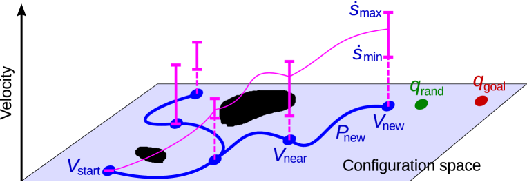
Figure 5: Illustration for AVP-RRT. The horizontal plane represents the configuration space while the vertical axis represents the path velocity space. Black areas represent configuration space obstacles. A vertex in the tree is composed of a configuration (blue disks), the incoming path from the parent (blue curve), and the interval of admissible velocities (bold magenta segments). At each tree extension step, one interpolates a smooth, collision-free path in the configuration space and propagates the interval of admissible velocities along that path using AVP. The fine magenta line shows one possible valid velocity profile (which is guaranteed to exist by AVP) “above” the path connecting $\mathbf{q}_{\mathrm{start}}$ and $\mathbf{q}_{\mathrm{new}}$.

Input : $\mathcal{T}$, $\mathbf{q}_{\mathrm{rand}}$

Output : A new vertex $V_{\mathrm{new}}$ or Null

1:  $V_{\mathrm{near}}\leftarrow$ NEAREST_NEIGHBOR($\mathcal{T},\mathbf{q}_{\mathrm{rand}}$)

2:  $(\mathcal{P}_{\mathrm{new}},\mathbf{q}_{\mathrm{new}})\leftarrow$ INTERPOLATE($V_{\mathrm{near}},\mathbf{q}_{\mathrm{rand}}$)

3:  if $\mathcal{P}$ is collision-free then

4:     $[\dot{s}_{\min},\dot{s}_{\max}]\leftarrow$ AVP($\mathcal{P}_{\mathrm{new}},V_{\mathrm{near}}.\mathrm{interval}$)

5:     if AVP succeeds then

6:        $V_{\mathrm{new}}\leftarrow$ NEW_VERTEX()

7:        $V_{\mathrm{new}}.\mathrm{config}\leftarrow\mathbf{q}_{\mathrm{new}}$; $V_{\mathrm{new}}.\mathrm{inpath}\leftarrow\mathcal{P}_{\mathrm{new}}$; $V_{\mathrm{new}}.\mathrm{interval}\leftarrow[\dot{s}_{\min},\dot{s}_{\max}]$

8:        return  $V_{\mathrm{new}}$

9:     end if

10:  end if

11:  return  Failure

Box 3 EXTEND

The other routines are defined as follows :

• CONNECT($V,\mathbf{q}_{\mathrm{goal}}$) attempts at connecting directly $V$ to the goal configuration $\mathbf{q}_{\mathrm{goal}}$, using the same algorithm as in lines 2 to 10 of Box 3, but with the further requirement that the goal velocity is included in the final velocity interval;

• COMPUTE_TRAJECTORY($\mathcal{T},\mathbf{q}_{\mathrm{goal}}$) reconstructs the entire path $\mathcal{P}_{\textrm{total}}$ from $\mathbf{q}_{\mathrm{start}}$ to $\mathbf{q}_{\mathrm{goal}}$ by recursively concatenating the $V$.inpath. Next, $\mathcal{P}_{\textrm{total}}$ is time-parameterized by applying TOPP. The existence of a valid time-parameterization is guaranteed by recursion by AVP.

• NEAREST_NEIGHBOR($\mathcal{T},\mathbf{q}$) returns the vertex of $\mathcal{T}$ whose configuration is closest to configuration $\mathbf{q}$ in the metric $d$, see Section 3.2 for a more detailed discussion.

• INTERPOLATE($V,\mathbf{q}$) returns a pair $(\mathcal{P}_{\mathrm{new}},\mathbf{q}_{\mathrm{new}})$ where $\mathbf{q}_{\mathrm{new}}$ is defined as follows

  • if $d(V$.config,$\mathbf{q})\leq R$ where $R$ is a user-defined extension radius as in the standard RRT algorithm (Kuffner and LaValle, 2000), then $\mathbf{q}_{\mathrm{new}}\leftarrow\mathbf{q}$;

  • otherwise, $\mathbf{q}_{\mathrm{new}}$ is a configuration “in the direction of” $\mathbf{q}$ but situated within a distance $R$ of $V$.config (contrary to the standard RRT, it might not be wise to choose a configuration laying exactly on the segment connecting $V$.config and $\mathbf{q}$ since here one has also to take care of $C^{1}$-continuity, see below).

  The path $\mathcal{P}_{\mathrm{new}}$ is a smooth path connecting $V$.config and $\mathbf{q}_{\mathrm{new}}$, and such that the concatenation of $V$.inpath and $\mathcal{P}_{\mathrm{new}}$ is $C^{1}$ at $V$.config, see Section 3.2 for a more detailed discussion.

3.2 Implementation and variations

As in the standard RRT (Kuffner and LaValle, 2000), some implementation choices influence substantially the performance of the algorithm.

Metric

In state-space RRTs, the most critical choice is that of the metric $d$, in particular, the relative weighting between configuration-space coordinates and velocity coordinates. In our approach, since the whole interval of valid path velocities is considered, the relative weighting does not come into play. In practice, a simple Euclidean metric on the configuration space is often sufficient. However, in some applications, one may also include the final orientation of $V$.inpath in the metric.

Interpolation

In geometric path planners, the interpolation between two configurations is usually done using a straight segment. Here, since one needs to propagate velocities, it is necessary to enforce $C^{1}$-continuity at the junction point. In the examples of Section 4, we used third-degree polynomials to do so. Other interpolation methods are possible : higher-order polynomials, splines, etc. The choice of the appropriate method depends on the application and plays an important role in the performance of the algorithm.

K-nearest-neighbors

Attempting connection from $K$ nearest neighbors, where $K>1$ is a judiciously chosen parameter, has been found to improve the performance of RRT. To implement this, it suffices to replace line 2 of Box 3 with a FOR loop that enumerates the $K$ nearest neighbors. Note that this procedure is geared towards reducing the search time, not at improving the trajectory quality as in RRT^∗ (Karaman and Frazzoli, 2011), see also below.

Post-processing

After finding a solution trajectory, one can improve its quality (e.g. trajectory duration, trajectory smoothness, etc.), by repeatedly applying the following shortcutting procedure (Geraerts and Overmars, 2007; Pham, 2012):

1. select two random configurations on the trajectory;

2. interpolate a smooth shortcut path between these two configurations;

3. time-parameterize the shortcut using TOPP;

4. if the time-parameterized shortcut has shorter duration than the initial segment, then replace the latter by the former.

Instead of shortcutting, one may also give the trajectory found by AVP-RRT as initial guess to a trajectory optimization algorithm, or implement a re-wiring procedure as in RRT^∗ (Karaman and Frazzoli, 2011), which has been shown to be asymptotically optimal in the context of state-based planning (note however that such re-wiring is not straightforward and might require additional algorithmic developments).

Another significant benefit of AVP is that one can readily adapt heuristics that have been developed for geometric path planners. We discuss two such heuristics below.

Bi-directional RRT

Kuffner and LaValle (2000) remarked that growing simultaneously two trees, one rooted at the initial configuration and one rooted at the goal configuration yielded significant improvement over the classical uni-directional RRT. This idea (see also Nakamura and Mukherjee, 1991) can be easily implemented in the context of AVP-RRT as follows (Lertkultanon and Pham, 2014) :

• The start tree is grown normally as in Section 3.1;

• The goal tree is grown similarly, but using AVP-backward (see Section 2.3) for the velocity propagation step;

• Assume that one finds a configuration where the two trees are geometrically connected. If the forward velocity interval of the start tree and the backward velocity interval of the goal tree have a non-empty intersection at this configuration, then the two trees can be connected dynamically.

Bridge test

If two nearby configurations are in the obstacle space but their midpoint $\mathbf{q}$ is in the free space, then most probably $\mathbf{q}$ is in a narrow passage. This idea enables one to find a large number of such configurations $\mathbf{q}$, which is essential in problems involving narrow passages (Hsu et al., 2003). This idea can be easily implemented in AVP-RRT by simply modifying RANDOM_CONFIG in line 6 of Box 2 to include the bridge test.

One can observe from the above discussion that powerful heuristics developed for geometric path planning can be readily used in AVP-RRT, precisely because the latter is built on the idea of path-velocity decomposition. It is unclear how such heuristics can be integrated in other approaches to kinodynamic motion planning such as the trajectory optimization approach discussed in the Introduction.

4 Examples of applications

As AVP-RRT is based on the classical Time-Optimal Path Parameterization (TOPP) algorithm, it can be applied to any type of systems and constraints TOPP can handle, from double-integrators subject to velocity and acceleration bounds, to manipulator subject to torque limits (Bobrow et al., 1985; Shin and McKay, 1986), to wheeled vehicles subject to balance constraints (Shiller and Gwo, 1991), to humanoid robots in multi-contact tasks (Pham and Stasse, 2015), etc. Furthermore, the overhead for addressing a new problem is minimal : it suffices to reduce the system constraints to the form of inequality (1), and le tour est joué!

In this section, we present two examples where AVP-RRT was used to address planning problems in which no quasi-static solution exists. In the first example, the task consisted in swinging a double pendulum into the upright configuration under severe torque bounds. While this example does not fully exploit the advantages associated with path-velocity decomposition (no configuration-space obstacle nor kinematic closure constraint was considered), we chose it since it was simple enough to enable a careful comparison with the usual state-space planning approach (LaValle and Kuffner, 2001). In the second example, the task consisted in transporting a bottle placed on a tray through a small opening using a commercially-available manipulator (6 DOFs). This example demonstrates the full power of path-velocity decomposition : geometric constraints (going through the small opening) and dynamics constraints (the bottle must remain on the tray) could be addressed separately. To the best of our knowledge, this is the first successful demonstration on a non custom-built robot that kinodynamic planning can succeed where quasi-static planning is guaranteed to fail.

4.1 Double pendulum with severe torque bounds

We first consider a fully-actuated double pendulum (see Figure 6B), subject to torque limits

$$|\tau_{1}|\leq\tau_{1}^{\max},\qquad|\tau_{2}|\leq\tau_{2}^{\max}.$$

Such a pendulum can be seen as a 2-link manipulator, so that the reduction to the form of (1) is straightforward, see Pham (2014).

4.1.1 Obstruction to quasi-static planning

The task consisted in bringing the pendulum from its initial state $(\theta_{1},\theta_{2},\dot{\theta}_{1},\dot{\theta}_{2})=(0,0,0,0)$ towards the upright state $(\theta_{1},\theta_{2},\dot{\theta}_{1},\dot{\theta}_{2})=(\pi,0,0,0)$, while respecting the torque bounds. For simplicity, we did not consider self-collision issues.

Any trajectory that achieves the task must pass through a configuration where $\theta_{1}=\pi/2$. Note that the configuration with $\theta_{1}=\pi/2$ that requires the smallest torque at the first joint to stay still is $(\theta_{1},\theta_{2})=(\pi/2,\pi)$. Let then $\tau_{1}^{\mathrm{qs}}$ be this smallest torque. It is clear that, if $\tau_{1}^{\max}<\tau_{1}^{\mathrm{qs}}$, then no quasi-static trajectory can achieve the task.

In our simulations, we used the following lengths and masses for the links: $l=0.2$ m and $m=8$ kg, yielding $\tau_{1}^{\mathrm{qs}}=15.68$ N$\cdot$m. For information, the smallest torque at the second joint to keep the configuration $(\theta_{1},\theta_{2})=(0,\pi/2)$ stationary was $7.84$ N$\cdot$m. We carried experiments in the following scenarii: $(\tau_{1}^{\max},\tau_{2}^{\max})\in\{(11,7),(13,5),(11,5)\}$ (N$\cdot$m).

4.1.2 Solution using AVP-RRT

For simplicity we used the uni-directional version of AVP-RRT as described in Section 3, without any heuristics. Furthermore, for fair comparison with state-space RRT in Python (see Section 4.1.3), we used a Python implementation of AVP rather than the C++ implementation contained in the TOPP library (Pham, 2014).

Regarding the number of nearest neighbors to consider, we chose $K=10$. The maximum number of repetitions was set to $N_{\mathrm{maxrep}}=2000$. Random configurations were sampled uniformly in $[-\pi,\pi]^{2}$. A simple Euclidean metric in the configuration space was used. Inverse Dynamics computations (required by the TOPP algorithm) were performed using OpenRAVE (Diankov, 2010). We ran 40 simulations for each value of $(\tau_{1}^{\max},\tau_{2}^{\max})$ on a 2 GHz Intel Core Duo computer with 2 GB RAM. The results are given in Table 1 and Figure 6. A video of some successful trajectories are shown at http://youtu.be/oFyPhI3JN00.

Table 1: Results for the pendulum simulations

$\tau^{\max}$	Success	Configs	Vertices	Search time
(N$\cdot$m)	rate	tested	added	(min)
(11,7)	100%	64$\pm$44	31$\pm$23	4.2$\pm$2.7
(13,5)	100%	92$\pm$106	29$\pm$30	5.9$\pm$6.3
(11,5)	92.5%	212$\pm$327	56$\pm$81	12.1$\pm$15.0

A                                           B

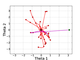
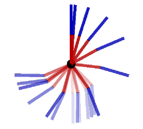
C                                           D

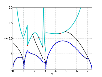
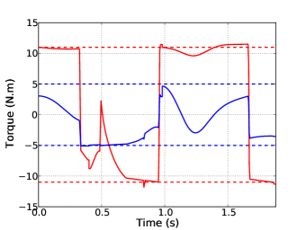
Figure 6: Swinging up a fully-actuated double pendulum. A typical solution for the case $(\tau_{1}^{\max},\tau_{2}^{\max})=(11,5)$ N$\cdot$m, with trajectory duration 1.88 s (see also the attached video). A: The tree in the $(\theta_{1},\theta_{2})$ space. The final path is highlighted in magenta. B: snapshots of the trajectory, taken every 0.1 s. Snapshots taken near the beginning of the trajectory are lighter. A video of the movement is available at http://youtu.be/oFyPhI3JN00. C: Velocity profiles in the $(s,\dot{s})$ space. The MVC is in cyan. The various velocity profiles (CLC, $\Phi$, $\Psi$, cf. Section 2.2) are in black. The final, optimal, velocity profile is in dashed blue. The vertical dashed red lines correspond to vertices where 0 is a valid velocity, which allowed a discontinuity of the path tangent at that vertex. D: Torques profiles. The torques for joint 1 and 2 are respectively in red and in blue. The torque limits are in dotted line. Note that, in agreement with time-optimal control theory, at each time instant, at least one torque limit was saturated (the small overshoots were caused by discretization errors).

4.1.3 Comparison with state-space RRT

We compared our implementation of AVP-RRT with the standard state-space RRT (LaValle and Kuffner, 2001) including the $K$-nearest-neighbors heuristic ($K$NN-RRT). More complex kinodynamic planners have been applied to low-DOF systems like the double pendulum, in particular those based on locally linearized dynamics (such as LQR-RRT^∗ Perez et al., 2012). However, such planners require delicate tunings and have not been shown to scale to systems with DOF $\geq$ 4. The goal of the present section is to compare the behavior of AVP-RRT to its RRT counterpart on a low-DOF system. (In particular, we do not claim that AVP-RRT is the best planner for a double pendulum.)

We equipped the state-space RRT with generic heuristics that we tuned to the problem at hand, see Appendix A. In particular, we selected the best number of neighbors $K$ for $K\in\{1,10,40,100\}$. Figure 7 and Table 2 summarize the results.

A                                                    B

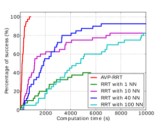
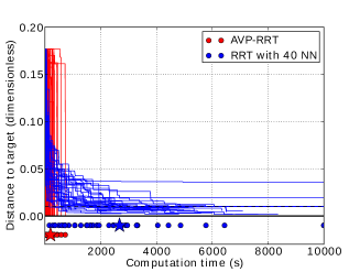
C                                                    D

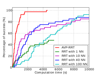
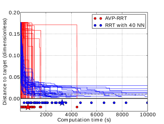
Figure 7: Comparison of AVP-RRT and $K$NN-RRT. A : Percentage of trials that have reached the goal area at given time instants for $\tau^{\max}=(11,7)$. B : Individual plots for each trial. Each curve shows the distance to the goal as a function of time for a given instance (red: AVP-RRT, blue: RRT-40). Dots indicate the time instants when a trial successfully terminated. Stars show the mean values of termination times. C and D : same legends as A and B but for $\tau^{\max}=(11,5)$.

Table 2: Comparison of AVP-RRT and $K$NN-RRT

	$\tau^{\max}=(11,7)$		$\tau^{\max}=(11,5)$
Planner	Success	Search time	Success	Search time
	rate	(min)	rate	(min)
AVP-RRT	100%	3.3$\pm$2.6	100%	9.8$\pm$12.1
RRT-1	40%	70.0$\pm$34.1	47.5%	63.8$\pm$36.6
RRT-10	82.5%	53.1$\pm$59.5	85%	56.3$\pm$60.1
RRT-40	92.5%	44.6$\pm$42.6	87.5%	54.6$\pm$52.2
RRT-100	82.5%	88.4$\pm$54.0	92.5%	81.2$\pm$46.7

In the two problem instances, AVP-RRT was respectively 13.4 and 5.6 times faster than the best $K$NN-RRT in terms of search time. We noted however that the search time of AVP-RRT increased significantly from instance $(\tau^{\max}_{1},\tau^{\max}_{2})=(11,5)$ to instance $(\tau^{\max}_{1},\tau^{\max}_{2})=(11,7)$, while that of RRT only marginally increased. This may be caused by the “superposition” phenomenon : as torque constraints become tighter, more “pumping” swings are necessary to reach the upright configuration. However, since our metric was only on the configuration-space variables, configurations with different speeds (corresponding to different pumping cycles) may become indistinguishable. While this problem could be addressed by including a measure of reachable velocity intervals into the metric, we chose not to do so in the present paper in order to avoid over-fitting our implementation of AVP-RRT to the problem at hand. Nevertheless, AVP-RRT still significantly over-performed the best $K$NN-RRT.

4.2 Non-prehensile object transportation

Here we consider the non-prehensile (i.e. without grasping) transportation of a bottle, or “waiter motion”. Non-prehensile transportation can be faster and more efficient than prehensile transportation since the time-consuming grasping and un-grasping stages are entirely skipped. Moreover, in many applications, the objects to be carried are too soft, fragile or small to be adequately grasped (e.g. food, electronic components, etc.)

4.2.1 Obstruction to quasi-static planning

A plastic milk bottle partially filled with sand was placed (without any fixation device) on a tray. The mass of the bottle was 2.5 kg, its height was 24 cm (the sand was filled up to 16 cm) and its base was a square of size 8 cm $\times$ 8 cm. The tray was mounted as the end-effector of a 6-DOF serial manipulator (Denso VS-060). The task consisted in bringing the bottle from an initial configuration towards a goal configuration, these two configurations being separated by a small opening (see Fig. 8A).

For the bottle to remain stationary with respect to the tray, the following three conditions must be satisfied :

• (Unilaterality) The normal component $f_{n}$ of the reaction force must be non-negative;

• (Non-slippage) The tangential component $\mathbf{f}_{t}$ of the reaction force must satisfy $\|\mathbf{f}_{t}\|\leq\mu f_{n}$, where $\mu$ is the static friction coefficient between the bottle and the tray. In our experimental set-up, the friction coefficient was set to a high value ($\mu=1.7$), such that the non-slippage condition was never violated before the ZMP condition;

• (ZMP) The ZMP of the bottle must lie inside the bottle base (Vukobratovic et al., 2001).

The height of the opening was designed so that, for the bottle to go through the opening, it must be tilted by at least an angle $\theta^{\mathrm{qs}}$. However, when the bottle is tilted by that angle, the center of mass (COM) of the bottle projects outside of the bottle base. As the projection of the COM coincides with the ZMP in the quasi-static condition, tilting the bottle by the angle $\theta^{\mathrm{qs}}$ thus violates the ZMP condition and as a result, the bottle will tip over. One can therefore conclude that no quasi-static motion can bring the bottle through the opening without tipping it over.

4.2.2 Solution using AVP-RRT

We first reduced the three aforementioned conditions to the form of (1). Details of this reduction can be found in Lertkultanon and Pham (2014). We next used the bi-directional version of AVP-RRT presented in Section 3.2. All vertices in the tree were considered for possible connection from a new random configuration, but they were sorted by increasing distance from the new configuration (a simple Euclidean metric in the configuration space was used for the distance computation). As the opening was very small (narrow passage), we made use of the bridge test (Hsu et al., 2003) in order to automatically sample a sizable number of configurations inside or close to the opening. Note that the use of the bridge test was natural thanks to path-velocity decomposition.

Because of the discrepancy between the planned motion and the motion actually executed on the robot (in particular, actual acceleration switches cannot be infinitely fast), we set the safety boundaries to be a square of size 5.5 cm $\times$ 5.5 cm (the actual base size was 8 cm $\times$ 8 cm), which makes the planning problem even harder. Nevertheless, our algorithm was able to find a feasible movement in about 3 hours on a 3.2 GHz Intel Core computer with 3.8 GB RAM (see Fig. 8B–E), and this movement could be successfully executed on the actual robot, see Fig. 9 and the video at http://youtu.be/LdZSjNwpJs0. Note that the computation time of 3 hours was for a particularly difficult problem instance : if the opening was only 5 cm higher, computation time would be about 2 minutes, see Fig. 8F.

A                                     B                                     C

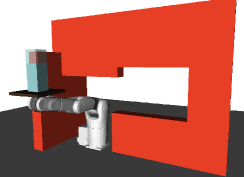
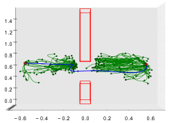
D                                     E                                     F

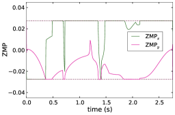
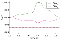
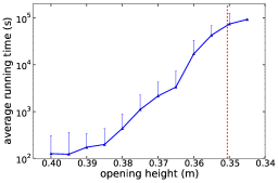
Figure 8: Non-prehensile transportation of a bottle. A : Simulation environment. The robot must bring the bottle to the other side of the opening while keeping it balanced on the tray. B : Bi-RRT tree in the workspace : the start tree had 125 vertices and the goal tree had 116 vertices. Red boxes represent the obstacles. Red stars represent the initial and goal positions of the bottle COM. Green lines represent the paths of the bottle COM in the tree. The successful path is highlighted in blue : it had 6 vertices. C : MVC and velocity profiles in the $(s,\dot{s})$ space. Same legend as in Fig. 6C. D : ZMP of the bottle in the tray reference frame (RF) for the successful trajectory. Note that the ZMP always stayed within the imposed safety borders $\pm 2.75$ cm (the actual borders were $\pm 4$ cm). E : COM of the bottle in the tray RF for the successful trajectory. Note that the X-coordinate of the COM reached the maximum value of 4.03 cm, around the moment when the bottle went through the opening, indicating that the successful trajectory would not be quasi-statically feasible. F : Here we varied the opening height (X-axis, from left to right : higher opening to lower opening) and determine the average and standard deviation of computation time (Y-axis, logarithmic scale) required to find a solution. We carried out 30 runs for opening heights from 0.4m to 0.365m, 10 runs for 0.36m, 3 runs for 0.355m and 0.35m and 2 runs for 0.345m. The red dashed vertical line indicates the critical height below which no quasi-static trajectory was possible. Here, we used $\pm 4$ cm as boundaries for the ZMP, so that the computed motions, while theoretically feasible, might not be actually feasible.

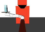
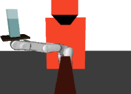
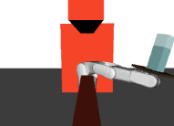
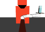
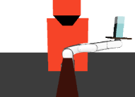
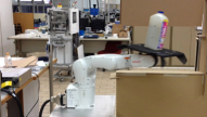
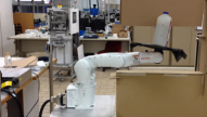
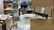
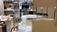
Figure 9: Snapshots of the motion of Fig. 8B–E taken every 0.5 s. Top two rows : front view of the motion in the simulation environment. Bottom two rows : side view of the motion executed on the actual robot (see also the video at http://youtu.be/LdZSjNwpJs0).

4.2.3 Comparison with OMPL-KPIECE

We were interested in comparing AVP-RRT with a state-of-the-art planner on this bottle-and-tray problem. We chose KPIECE since it is one of the most generic and powerful existing kinodynamic planners (Sucan and Kavraki, 2012). Moreover, a robust open-source implementation exists as a component of the widely-used Open Motion Planning Library (OMPL) (Sucan et al., 2012).

The methods and results of the comparison are reported in detail in Appendix C. Briefly, we first fine-tuned OMPL-KPIECE on the same 6-DOF manipulator model as above. At this stage, we considered only bounds on velocity and accelerations, the bottle and the tray were ignored for simplicity. Next, we compared AVP-RRT (Python/C++) and OMPL-KPIECE (pure C++, with the best possible tunings obtained previously) in an environment similar to that of Fig. 8. Here, we considered bounds on velocity and accelerations and collisions with the environment. We ran each planner 20 times with a time limit of 600 seconds. AVP-RRT had a success rate of $100\%$ and an average running time of $68.67$ s, while OMPL-KPIECE failed to find any solution in any run. Based on this decisive result, we decided not to try OMPL-KPIECE on the full bottle-and-tray problem.

These comparison results thus further suggest that planning directly in the state-space, while interesting from a theoretical viewpoint and successful in simulations and/or on custom-built systems, is unlikely to scale to practical high-DOF problems.

5 Discussion

We have presented a new algorithm, Admissible Velocity Propagation (AVP) which, given a path and an interval of reachable velocities at the beginning of that path, computes exactly and efficiently the interval of valid final velocities. We have shown how to combine AVP with well-known sampling-based geometric planners to give rise to a family of new efficient kinodynamic planners, which we have evaluated on two difficult kinodynamic problems.

Comparison to existing approaches to kinodynamic planning

Compared to traditional planners based on path-velocity decomposition, our planners remove the limitation of quasi-static feasibility, precisely by propagating admissible velocity intervals at each step of the tree extension. This enables our planner to find solutions when quasi-static trajectories are guaranteed to fail, as illustrated by the two examples of Section 4.

Compared to other approaches to kinodynamic planning, our approach enjoys the advantages associated with path-velocity decomposition, namely, the separation of the complex planning problem into two simpler sub-problems : geometric and dynamic, for both of which powerful methods and heuristics have been developed.

The bottle transportation example in Section 4.2 illustrates clearly this advantage. To address the problem of the narrow passage constituted by the small opening, we made use of the bridge test heuristics – initially developed for geometric path planners (Hsu et al., 2003) – which provides a large number of samples inside the narrow passage. It is unclear how such a method could be integrated into the “trajectory optimization” approach for example. Next, to steer between two configurations, we simply interpolated a geometric path – and can check for collision at this stage – and then found possible trajectories by running AVP. By contrast, in a “state-space planning” approach, it would be difficult – if not impossible – to steer exactly between two states of the system, which requires for instance solving a two-point boundary value problem. To avoid solving such difficult problems, LaValle and Kuffner (2001); Hsu et al. (2002) propose to sample a large number of time-series of random control inputs and to choose the time-series that steers the system the closest to the target state. However, such shooting methods are usually considerably slower than “exact” methods – which is the case of AVP –, as also illustrated in our simulation study (see Section 4.1 and Appendices B, C).

Class of systems where AVP is applicable

Since AVP is adapted from TOPP, AVP can handle all systems and constraints that TOPP can handle, and only those systems and constraints. Essentially, TOPP can be applied to a path $\mathbf{q}(s)$ in the configuration space if the system can track that path at any velocities $\dot{s}$ and accelerations $\ddot{s}$, subject only to inequality constraints on $\dot{s}$ and $\ddot{s}$. This excludes – a priori – all under-actuated robots since, for these robots, most of the paths in the configuration space cannot be traversed at all (Laumond, 1998), or at only one specific velocity. Bullo and Lynch (2001) identified a subclass of under-actuated robots (including e.g. planar 3-DOF manipulators with one passive joint or 3D underwater vehicles with three off-center thrusters) for which one can compute a large subset of paths that can be TOPP-ed (termed “kinematic motions”). Investigating whether AVP-RRT can be applied to such systems is the subject of ongoing research.

At the other end of the spectrum, redundantly-actuated robots can track most of the paths in their configuration space (again, subject to actuation bounds). The problem here is that, for a given admissible velocity profile along a path, there exists in general an infinity of combinations of torques that can achieve that velocity profile. Pham and Stasse (2015) showed how to optimally exploit actuation redundancy in TOPP, which can be adapted straightforwardly to AVP-RRT.

Further remarks on completeness and complexity

The AVP-RRT planner as presented in Section 3 is likely not probabilistically complete. We address in more detail in Appendix A the completeness properties of AVP-RRT, and more generally, of AVP-based planners.

We now discuss another feature of AVP-based planners that makes them interesting from a complexity viewpoint. Consider a trajectory or a trajectory segment that is “explored” by a state-space planning or a trajectory optimization method – either in one extension step for the former, or in an iterative optimization step for the latter. If one considers the underlying path of this trajectory, one may argue that these methods are exploring only one time-parameterization of that path, namely, that corresponding to the trajectory at hand. By contrast, for a given path that is “explored” by AVP, AVP precisely explores all time-parameterizations of that path, or in other words, the whole “fiber bundle” of path velocities above the path at hand – at a computation cost only slightly higher than that of checking one time-parameterization (see Section 2.3). Granted that path velocity encodes important information about possible violations of the dynamics constraints as argued in the Introduction, this full and free (as in free beer) exploration enables significant performance gains.

Future works

As just mentioned, we have recently extended TOPP to redundantly-actuated systems, including humanoid robots in multi-contact tasks (Pham and Stasse, 2015). This enables AVP-based planners to be applied to multi-contact planning for humanoid robots. In this application, the existence of kinematic closure constraints (the parts of the robot in contact with the environment should remain fixed) makes path-velocity decomposition highly appealing since these constraints can be handled by a kinematic planner independently from dynamic constraints (torque limits, balance, etc.) In a preliminary experiment, we have planned a non-quasi-statically-feasible but dynamically-feasible motion for a humanoid robot (see http://youtu.be/PkDSHodmvxY). Going further, we are currently investigating how AVP-based planners can enable existing quasi-static multi-contact planning methods (Hauser et al., 2008; Escande et al., 2013) to discover truly dynamic motions for humanoid robots with multiple contact changes.

Acknowledgments

We are grateful to Prof. Zvi Shiller for inspiring discussions about the TOPP algorithm and kinodynamic planning. This work was supported by a JSPS postdoctoral fellowship, by a Start-Up Grant from NTU, Singapore, and by a Tier 1 grant from MOE, Singapore.

Appendix A Probabilistic completeness of AVP-based planners

Essentially, the probabilistic completeness of AVP-based planners relies on two properties: the completeness of the path sampling process (Property 1), and the completeness of velocity propagation (Property 2)

Property 1

any smooth path $\mathcal{P}$ in the configuration space will be approximated arbitrarily closely by the sampling process for a sufficiently large number of samples;

Property 2

if a smooth path $\widehat{\mathcal{P}}=\hat{\mathbf{q}}(s)_{s\in[0,1]}$ obtained by the sampling process can be time-parameterized into a solution trajectory according to a certain velocity profile $\hat{v}$, then $\hat{v}$ is contained within the velocity band propagated by AVP.

We first discuss the conditions under which these two Properties are verified and then establish the completeness of AVP-based planners.

Definition 3

Let $d$ designate a $\mathcal{L}^{\infty}$-type distance between two trajectories or between two paths :

$$d(\Pi,\widehat{\Pi}) \stackrel{{\scriptstyle\mathrm{def}}}{{=}} \sup_{t\in[0,T]}\|\Pi(t)-\widehat{\Pi}(t)\|,$$ (9)

$$d(\mathcal{P},\widehat{\mathcal{P}}) \stackrel{{\scriptstyle\mathrm{def}}}{{=}} \sup_{s\in[0,1]}\|\mathbf{q}(s)-\widehat{\mathbf{q}}(s)\|+\sup_{s\in[0,1]}\|\mathbf{u}(s)-\widehat{\mathbf{u}}(s)\|,$$ (10)

where $\mathbf{u}(s)$ is the unit tangent vector to $\mathcal{P}$ at $s$.

Proposition 1

Property 1 is true under the following hypotheses on the sampling process

H1

each time a random configuration $\mathbf{q}_{\mathrm{rand}}$ is sampled, consider the set $\mathcal{S}$ of existing vertices within a distance $\delta>0$ of $\mathbf{q}_{\mathrm{rand}}$ in the configuration space. Select $K$ random vertices within $\mathcal{S}$, where $K$ is proportional to the number of vertices currently existing in the tree, and attempt to connect these vertices to $\mathbf{q}_{\mathrm{rand}}$ through the usual interpolation and AVP procedures. For each successful connection, create a new vertex $V_{\mathrm{new}}$, which has the same configuration $\mathbf{q}_{\mathrm{rand}}$ but a different “inpath” and a different “interval”, depending on the parent vertex in $\mathcal{S}$ ;

H2

consider the path interpolation from $(\mathbf{u}_{1},\mathbf{q}_{1})$ to $\mathbf{q}_{2}$. The unit vector $\mathbf{u}_{2}$ at the end of the interpolated path $\mathcal{P}_{\mathrm{int}}$ is set to be the unit vector pointing from $\mathbf{q}_{1}$ to $\mathbf{q}_{2}$, denoted $\mathbf{u}_{\mathbf{q}_{1}\to\mathbf{q}_{2}}$ ;

H3

for every $\Delta>0$, there exists $\eta>0$ such that, if $\|\mathbf{u}_{1}-\mathbf{u}_{\mathbf{q}_{1}\to\mathbf{q}_{2}})\|<\eta$, then $d(\mathcal{P}_{\mathrm{int}},\mathcal{P}_{\mathrm{str}}(\mathbf{q}_{1},\mathbf{q}_{2}))<\Delta/3$, where $\mathcal{P}_{\mathrm{str}}(\mathbf{q}_{1},\mathbf{q}_{2})$ is the straight segment joining $\mathbf{q}_{1}$ to $\mathbf{q}_{2}$ .

Proof Consider a smooth path $\mathcal{P}=\mathbf{q}(s)_{s\in[0,1]}$ in the configuration space such that $\mathbf{q}(0)=\mathbf{q}_{\mathrm{start}}$. Since $\mathcal{P}$ is smooth, for $s_{1}$ and $s_{2}$ close enough, the path segment between $s_{1}$ and $s_{2}$ will look like a straight line, see Fig. 10B. This intuition can be more formally stated as follows: consider an arbitrary $\Delta>0$,

• there exists a $\delta_{1}$ such that, if $\|\mathbf{q}(s_{2})-\mathbf{q}(s_{1})\|\leq\delta_{1}$, then

  $$d(\mathbf{q}(s)_{s\in[s_{1},s_{2}]},\mathcal{P}_{\mathrm{str}}(\mathbf{q}(s_{1}),\mathbf{q}(s_{2})))<\Delta/3;$$ (11)

• there exists $\delta_{2}$ such that, if $\|\mathbf{q}(s_{2})-\mathbf{q}(s_{1})\|\leq\delta_{2}$, then

  $$\|\mathbf{u}(s_{1})-\mathbf{u}_{\mathbf{q}(s_{1})\to\mathbf{q}(s_{2})})\|<\eta/6\quad\textrm{and}\quad\|\mathbf{u}(s_{2})-\mathbf{u}_{\mathbf{q}(s_{1})\to\mathbf{q}(s_{2})})\|<\eta/6,$$ (12)

  where $\eta$ is defined in (H3).

A                                                            B
  

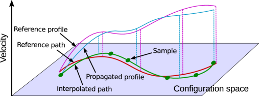
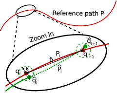
Figure 10: Completeness of AVP-RRT. A : Existence of an admissible velocity profile above an approximated path. B : Approximation of a given smooth path.

Divide now the path $\mathcal{P}$ into $n$ subpaths $\mathcal{P}_{1}$,…,$\mathcal{P}_{n}$ of lengths approximately $\delta\stackrel{{\scriptstyle\mathrm{def}}}{{=}}\min(\delta_{1},\delta_{2})$. Let $\mathbf{q}_{i},\mathbf{u}_{i}$ denote the starting configuration and unit tangent vector of subpath $\mathcal{P}_{i}$. Consider the balls $B_{i}$ centered on the $\mathbf{q}_{i}$ and having radius $\epsilon$, where $\epsilon\stackrel{{\scriptstyle\mathrm{def}}}{{=}}\frac{\eta\delta}{12}$. With probability 1, there will exist a time in the sampling process when

(s1)

$n$ consecutive random configurations $\hat{\mathbf{q}}_{1},\dots,\hat{\mathbf{q}}_{1}$ are sampled in $B_{1},\dots,B_{n}$ respectively;

(s2)

$\mathbf{q}_{\mathrm{start}}$ is selected for connection attempt towards $\hat{\mathbf{q}}_{1}$, and the random $\mathbf{u}_{\mathrm{start}}$ verifies $\|\mathbf{u}_{\mathrm{start}}-\mathbf{u}_{\mathbf{q}_{\mathrm{start}}\to\mathbf{q}_{1}}\|<2\eta/3$. The interpolation results in a new vertex $V_{1}$ and a new subpath $\widehat{\mathcal{P}}_{1}$ connecting $\mathbf{q}_{\mathrm{start}}$ to $V_{1}$;

(s3)

for $i\in[1,n-1]$, $V_{i}$ is selected for connection attempt to $\hat{\mathbf{q}}_{i+1}$, resulting in a new vertex $V_{i+1}$ and a new subpath $\widehat{\mathcal{P}}_{i}$ connecting $V_{i}$ to $V_{i+1}$.

Note that (s2) and (s3) are possible since, by (H1), the number of connection attempts $K$ grows linearly with the number of existing vertices in the tree.

We first prove that, for all $i\in[0,n]$, we have $\|\hat{\mathbf{u}}_{i}-\mathbf{u}_{i}\|<2\eta/3$. At rank $0$, the property is true owing to (s2). For $i\geq 1$, we have

• $\|\hat{\mathbf{u}}_{i}-\mathbf{u}_{\hat{\mathbf{q}}_{i-1}\to\hat{\mathbf{q}}_{i}}\|=0$ by (H2);

• $\|\mathbf{u}_{\hat{\mathbf{q}}_{i-1}\to\hat{\mathbf{q}}_{i}}-\mathbf{u}_{\mathbf{q}_{i-1}\to\mathbf{q}_{i}}\|<2\epsilon/\delta=\eta/6$ by the fact that each $\mathbf{q}_{i}$ is contained in the ball $B_{i}$;

• $\|\mathbf{u}_{\mathbf{q}_{i-1}\to\mathbf{q}_{i}}-\mathbf{u}_{i}\|<\eta/6$ by (12).

Applying triangle inequality yields $\|\hat{\mathbf{u}}_{i}-\mathbf{u}_{i}\|<2\eta/3$.

Next, we prove for all $i\in[0,n-1]$ that $d(\widehat{\mathcal{P}}_{i},\mathcal{P}_{i})<\Delta$. Note that

• $\|\hat{\mathbf{u}}_{i}-\mathbf{u}_{i}\|<2\eta/3$ by the above reasoning;

• $\|\mathbf{u}_{i}-\mathbf{u}_{\mathbf{q}_{i}\to\mathbf{q}_{i+1}}\|<\eta/6$ by (12);

• $\|\mathbf{u}_{\mathbf{q}_{i}\to\mathbf{q}_{i+1}}-\mathbf{u}_{\hat{\mathbf{q}}_{i}\to\hat{\mathbf{q}}_{i+1}}\|<2\epsilon/\delta=\eta/6$ by the fact that each $\mathbf{q}_{i}$ is contained in the ball $B_{i}$.

Thus, by triangle inequality, we have $\|\hat{\mathbf{u}}_{i}-\mathbf{u}_{\hat{\mathbf{q}}_{i}\to\hat{\mathbf{q}}_{i+1}}\|<\eta$. By (H3), we have $d(\widehat{\mathcal{P}}_{i},\mathcal{P}_{\mathrm{str}}(\hat{\mathbf{q}}_{1},\hat{\mathbf{q}}_{2}))<\Delta/3$. Next, $d(\mathcal{P}_{\mathrm{str}}(\hat{\mathbf{q}}_{1},\hat{\mathbf{q}}_{2}),\mathcal{P}_{\mathrm{str}}(\mathbf{q}_{1},\mathbf{q}_{2}))$ can be made smaller than $\Delta/3$ for judicious choices of $\epsilon$ and $\delta$. Finally, we have $d(\mathcal{P}_{i},\mathcal{P}_{\mathrm{str}}(\mathbf{q}(s_{1}),\mathbf{q}(s_{2})))<\Delta/3$ by (11). Applying the triangle inequality again, we obtain $d(\widehat{\mathcal{P}}_{i},\mathcal{P}_{i})<\Delta$. $\Box$

Proposition 2

Property 2 is true.

Proof Consider a path $\widehat{\mathcal{P}}$ obtained by the sampling process, i.e. $\widehat{\mathcal{P}}$ is composed of $n$ interpolated path segments $\widehat{\mathcal{P}}_{1}$,…,$\widehat{\mathcal{P}}_{n}$. Let $v_{1}$,…,$v_{n}$ be the corresponding subdivisions of the associated velocity profile $v$. We prove by induction on $i\in[0,n]$ that the concatenated profile $[v_{1},\dots,v_{i}]$ is contained within the velocity band propagated by AVP.

For $i=0$, i.e., at the start vertex, $v(0)=0$ is contained within the initial velocity band, which is $[0,0]$. Assume that the statement holds at $i$. This implies in particular that the final value of $v_{i}$, which is also the initial value of $v_{i+1}$, belongs to $[v_{\min},v_{\max}]$, where $(v_{\min},v_{\max})$ are the values returned by AVP at step $i$. Next, consider the velocity band that AVP propagates at step $i+1$ from $[v_{\min},v_{\max}]$. Since $v_{i+1}(0)\in[v_{\min},v_{\max}]$ and that $v_{i+1}$ is continuous, the whole profile $v_{i+1}$ will be contained, by construction, in the velocity band propagated by AVP. $\Box$

We can now prove the probabilistic completeness for a class of AVP-based planners.

Theorem 2

An AVP-based planner that verifies Properties 1 and 2 is probabilistically complete.

Proof Assume that there exists a smooth state-space trajectory $\Pi$ that solves the query, with $\Delta$-clearance in the state space, i.e., every smooth trajectory $\widehat{\Pi}$ such that $d(\Pi,\widehat{\Pi})\leq\Delta$ also solves the query . Let $\mathcal{P}$ be the underlying path of $\Pi$ in the configuration space. By Property 1, with probability 1, there exists a time when the sampling process will generate a smooth path $\widehat{\mathcal{P}}$ such that $d(\mathcal{P},\widehat{\mathcal{P}})\leq\Delta/2$. One can then construct, by continuity, a velocity profile $\hat{v}$ above $\widehat{\mathcal{P}}$, such that the time-parameterization of $\widehat{\mathcal{P}}$ according to $\hat{v}$ yields a trajectory $\widehat{\Pi}$ within a radius $\Delta$ of $\Pi$ (see Fig. 10A). As $\Pi$ has $\Delta$-clearance, $\widehat{\Pi}$ also solves the query. Thus, by Property 2, the velocity profile (or time-parameterization) $\hat{v}$ must be contained within the velocity band propagated by AVP, which implies finally that $\widehat{\mathcal{P}}$ can be successfully time-parameterized in the last step of the planner. $\Box$

Appendix B Comparison of AVP-RRT with $K$NN-RRT on a 2-DOF pendulum

Here, we detail the implementation of the standard state-space planner $K$NN-RRT and the comparison of this planner with AVP-RRT. The full source code for this comparison is available at https://github.com/stephane-caron/avp-rrt-rss-2013. Note that, for fairness, all the algorithms considered here were implemented in Python (including AVP). Thus, the presented computation times, in particular those of AVP-RRT, should not be considered in absolute terms.

B.1 $K$NN-RRT

B.1.1 Overall algorithm

Our implementation of RRT in the state-space (LaValle and Kuffner, 2001) is detailed in Boxes 4 and 5.

1:  $\mathcal{T}$.INITIALIZE($\mathbf{x}_{\mathrm{init}}$)

2:  for $\mathrm{rep}=1$ to $N_{\mathrm{max\_rep}}$ do

3:     $\mathbf{x}_{\mathrm{rand}}\leftarrow$ RANDOM_STATE() if mod(rep,5) $\neq 0$ else $\mathbf{x}_{\mathrm{goal}}$

4:     $\mathbf{x}_{\mathrm{new}}\leftarrow$ EXTEND($\mathcal{T},\mathbf{x}_{\mathrm{rand}}$)

5:     $\mathcal{T}$.ADD_VERTEX($\mathbf{x}_{\mathrm{new}}$)

6:     $\mathbf{x}_{\mathrm{new}2}\leftarrow$ EXTEND($\mathbf{x}_{\mathrm{new}},\mathbf{x}_{\mathrm{goal}}$)

7:     if $d(\mathbf{x}_{\mathrm{new}},\mathbf{x}_{\mathrm{goal}})\leq\epsilon$ or $d(\mathbf{x}_{\mathrm{new}2},\mathbf{x}_{\mathrm{goal}})\leq\epsilon$ then

8:        return  Success

9:     end if

10:  end for

11:  return  Failure

Box 4 $K$NN_RRT$(\mathbf{x}_{\mathrm{init}},\mathbf{x}_{\mathrm{goal}})$

1:  for $k=1$ to $K$ do

2:     $\mathbf{x}_{\mathrm{near}}^{k}\leftarrow$ KTH_NEAREST_NEIGHBOR($\mathcal{T},\mathbf{x}_{\mathrm{rand}},k$)

3:     $\mathbf{x}_{\mathrm{new}}^{k}\leftarrow$ STEER($\mathbf{x}_{\mathrm{near}}^{k},\mathbf{x}_{\mathrm{rand}}$)

4:  end for

5:  return  $\arg\min_{k}d(\mathbf{x}_{\mathrm{new}}^{k},\mathbf{x}_{\mathrm{rand}})$

Box 5 EXTEND($\mathcal{T},\mathbf{x}_{\mathrm{rand}}$)

Steer-to-goal frequency

We asserted the efficiency of the following strategy: every five extension attempts, try to steer directly to $\mathbf{x}_{\mathrm{goal}}$ (by setting $\mathbf{x}_{\mathrm{rand}}=\mathbf{x}_{\mathrm{goal}}$ on line 3 of Box 4). See also the discussion in LaValle and Kuffner (2001), p. 387, about the use of uni-directional and bi-directional RRTs. We observed that the choice of the steer-to-goal frequency (every 5, 10, etc., extension attempts) did not significantly alter the performance of the algorithm, except when it is too large, e.g. once every two extension attempts.

Metric

The metric for the neighbors search in EXTEND (Box 5) and to assess whether the goal has been reached (line 7 of Box 4) was defined as:

$$d(\mathbf{x}_{a},\mathbf{x}_{b}) = d\left((\mathbf{q}_{a},\mathbf{v}_{a}),(\mathbf{q}_{b},\mathbf{v}_{b})\right)$$ (13)

$$= \frac{\sum_{j=1,2}{\sqrt{1-\cos({\mathbf{q}_{a}}_{j}-{\mathbf{q}_{b}}_{j})}}}{4}+\frac{\sum_{j=1,2}|{\mathbf{v}_{a}}_{j}-{\mathbf{v}_{b}}_{j}|}{4V_{\max}},$$

where $V_{\max}$ denotes the maximum velocity bound set in the random sampler (function RANDOM_STATE() in Box 4). This simple metric is similar to an Euclidean metric but takes into account the periodicity of the joint values.

Termination condition

We defined the goal area as a ball of radius $\epsilon=10^{-2}$ for the metric (13) around the goal state $\mathbf{x}_{\mathrm{goal}}$. As an example, $d(\mathbf{x}_{a},\mathbf{x}_{a})=\epsilon$ corresponds to a maximum angular difference of $\Delta q_{1}\approx 0.057$ rad $\approx~{}$3.24 degrees in the first joint.

This choice is connected to that of the integration time step (used e.g. in Forward Dynamics computations in section B.1.2), which we set to $\delta t=0.01$ s. Indeed, the average angular velocities we observed in our benchmark was around $\bar{V}~{}=~{}5$ rad.s^-1 for the first joint, which corresponds to an average instantaneous displacement $\bar{V}\cdot\delta t\approx 5.10^{-2}$ rad of the same order as $\Delta q_{1}$ above.

Nearest-neighbor heuristic

Instead of considering only extensions from the nearest neighbor, as has commonly been done, we considered the “best” extension from the $K$ nearest neighbors (line 5 in Box 5), i.e. the extension yielding the state closest to $\mathbf{x}_{\mathrm{rand}}$ for the metric $d$ (cf. Equation (13)).

B.1.2 Local steering

Regarding the local steering scheme (STEER on line 3 of Box 5), there are two main approaches, corresponding to the two sides of the equation of motion : state-based and control-based steering (Caron et al., 2014).

Control-based steering

In this approach, a control input $\tau(t)$ is computed first. It generates a given trajectory computable by forward dynamics. Because $\tau(t)$ is computed beforehand, there is no direct control on the end-state of the trajectory. To palliate this, the function $\tau(t)$ is then updated, with or without feedback on the end-state, until some satisfactory result is obtained or a computation budget is exhausted. For example, in works such as LaValle and Kuffner (2001); Hsu et al. (2002), random functions $u$ are sampled from the set of piecewise-constant functions. A number of them are tried and only the one bringing the system closest to the target is retained. Linear-Quadratic Regulation (Perez et al., 2012; Tedrake, 2009) is another example of control-based steering where the function $u$ is computed as the optimal policy for a linear approximation of the system dynamics (given a quadratic cost function).

In the present work, we followed the control-based approach from LaValle and Kuffner (2001); Hsu et al. (2002), as described by Box 6. The random control is a stationary $(\tau_{1},\tau_{2})$ sampled as:

$$(\tau_{1},\tau_{2})\ \sim\ {\cal U}([-\tau^{\max}_{1},\tau^{\max}_{1}]\times[-\tau^{\max}_{2},\tau^{\max}_{2}]).$$

where $\cal U$ denotes uniform sampling from a set. The random time duration $\Delta t$ is sampled uniformly in $[\delta t,\Delta t_{\max}]$ where $\Delta t_{\max}$ is the maximum duration of local trajectories (parameter to be tuned), and $\delta t$ is the time step for the forward dynamics integration (set to $\delta t=0.01$ s as discussed in Section B.1.1). The number of local trajectories to be tested, $N_{\mathrm{local\_trajs}}$, is also a parameter to be tuned.

1:  for $p=1$ to $N_{\mathrm{local\_trajs}}$ do

2:     $\mathbf{u}\leftarrow$ RANDOM_CONTROL($\tau^{\max}_{1},\tau^{\max}_{2}$)

3:     $\Delta t\leftarrow$ RANDOM_DURATION($\Delta t_{\max}$)

4:     $\mathbf{x}^{p}\leftarrow$ FORWARD_DYNAMICS($\mathbf{x}_{\mathrm{near}},\mathbf{u},\Delta t$)

5:  end for

6:  return  $\mathrm{argmin}_{p}d(\mathbf{x}^{p},\mathbf{x}_{\mathrm{rand}})$

Box 6 STEER($\mathbf{x}_{\mathrm{near}},\mathbf{x}_{\mathrm{rand}}$)

State-based steering

In this approach, a trajectory $\widetilde{\mathbf{q}}(t)$ is computed first. For instance, $\widetilde{\mathbf{q}}$ can be a Bezier curve matching the initial and target configurations and velocities. The next step is then to compute a control that makes the system track it. For fully- or over-actuated system, this can done using inverse dynamics. If no suitable controls exist, the trajectory is rejected. Note that both the space $\Im(\widetilde{\mathbf{q}})$ and timing $t$ impact the dynamics of the system, and therefore the existence of admissible controls. Bezier curves or B-splines will conveniently solve the spatial part of the problem, but their timing is arbitrary, which tends to result in invalid controls and needs to be properly cared for.

To enable meaningful comparisons with AVP-RRT, we considered the simple state-based steering described in Box 7. Trying to design the best possible nonlinear controller for the double pendulum would be out of the scope of this work, as it would imply either problem-specific tunings or substantial modifications to the core RRT algorithm (as done e.g. in Perez et al., 2012).

1:  for 10 trials of $T\sim{\cal U}([0.01,2.])$ do

2:     $\widetilde{\mathbf{q}}\leftarrow\textrm{INTERPOLATE}(T,\mathbf{x}_{\mathrm{near}},\mathbf{x}_{\mathrm{rand}})$

3:     $\widetilde{\tau}:=\textrm{INVERSE\_DYNAMICS}(\widetilde{\mathbf{q}}(t),\dot{\widetilde{\mathbf{q}}}(t),\ddot{\widetilde{\mathbf{q}}}(t))$

4:     $t^{\dagger}=\sup\{t||\widetilde{\tau}(t)|\leq\tau^{\max}\}$

5:     if $t^{\dagger}>0$ then

6:        return  $\widetilde{\mathbf{q}}(t^{\dagger})$

7:     end if

8:  end for

9:  return  failure

Box 7 STEER($\mathbf{x}_{\mathrm{near}},\mathbf{x}_{\mathrm{rand}}$)

Here, $\textrm{INTERPOLATE}(T,\mathbf{x}_{a},\mathbf{x}_{b})$ returns a third-order polynomial $P_{i}(t)$ such that $P_{i}(0)=\mathbf{q}_{ai},\ P^{\prime}_{i}(0)=\mathbf{v}_{ai},\ P_{i}(T)=\mathbf{q}_{bi},\ P_{i}^{\prime}(T)=\mathbf{v}_{bi}$, and our local planner tries 10 different values of $T$ between 0.01 s and 2 s. We use inverse dynamics at each time step of the trajectory to check if a control $\widetilde{\tau}(t)$ is within torque limits. The trajectory is cut at the first inadmissible control.

Comparing the two approaches

On the pendulum, state-based steering yielded RRTs with slower exploration speeds compared to control-based steering, as illustrated in Figure 11. This slowness is likely due to the uniform sampling in a wide velocity range $[-V_{\max},V_{\max}]$, which resulted in a large fraction of trajectories exceeding torque limits. However, despite a better exploration of the state space, trajectories from control-based steering systematically ended outside of the goal area. To palliate this, we added a subsequent step : from each state reached by control-based steering, connect to the goal area using state-based steering. Thus, if a state is reached that is not in the goal area but from which steering to goal is easy, this last step will take care of the final connection. However, this patch improved only marginally the success rate of the planner. In practice, trajectories from control-based steering tend to end at energetic states from which steering to goal is difficult. As such, we found that this steering approach was not performing well on the pendulum and turned to state-based steering.

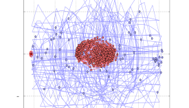
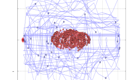
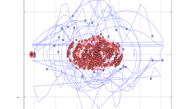
Figure 11: Comparison of control-based and state-based steering for $K=1$ (left-top), $K=10$ (right-top), $K=40$ (left-bottom) and $K=100$ (right-bottom). Computation time is fixed, which explains why there are more points for small values of $K$. The X-axis represents the angle of the first joint and the Y-axis its velocity. The trees grown by the state-based and control-based methods are in red and blue, respectively. The goal area is depicted by the red ellipse on the left side. Control-based steering yields better exploration of the state space, but fails to connect to the goal area.

Let us remark here that, although AVP-RRT follows the state-based paradigm (it indeed interpolates paths in configuration space and then computes feasible velocities along the path using Bobrow-like approach, which includes inverse dynamics computations), it is much more successful. The reason for this lies in AVP : when the interval of feasible velocities is small, a randomized approach will have a high probability of sampling unreachable velocities. Therefore, it will fail most of the time. Using AVP, the set of reachable velocities is exactly computed and this failure factor disappears. With AVP-RRT, failures only occur from “unlucky” sampling in the configuration space. Note however that the algorithm only saves and propagates the norm of the velocity vectors, not their directions, which may make the algorithm probabilistically incomplete (cf. discussion in Section 5).

B.1.3 Fine-tuning of $K$NN-RRT

Based on the above results, we now focus on $K$NN-RRTs with state-based steering for the remainder of this section. The parameters to be tuned are :

• $N_{\mathrm{local\_trajs}}$: number of local trajectories tested in each call to STEER;

• $\Delta t_{\max}$: maximum duration of each local trajectory.

The values we tested for these two parameters are summed up in table 3.

Number of trials	$N_{\mathrm{local\_trajs}}$	$\Delta t_{\max}$
10	1	0.2
10	30	0.2
10	80	0.2
20	20	0.5
20	20	1.0
20	20	2.0

Table 3: Parameter sets for each test.

The parameters we do not tune are :

• Maximum velocity $V_{\max}$ for sampling velocities. We set $V_{\max}=50$ rad.s^-1, which is about twice the maximum velocity observed in the successful trials of AVP-RRT;

• Number of neighbors $K$. In this tuning phase, we set $K=10$. Other values of $K$ will be tested in the final comparison with AVP in section B.2;

• Space-time precision $(\epsilon,\delta t)$: as discussed in Section B.1.1, we chose $\epsilon=0.01$ and $\delta t=0.01$ s.

Finally, in this tuning phase, we set the torque limit as $(\tau^{\max}_{1},\tau^{\max}_{2})=(13,7)$ N.m, which are relatively “slack” values, in order to obtain faster termination times for RRT. Tighter values such as $(\tau^{\max}_{1},\tau^{\max}_{2})=(11,5)$ N.m will be tested in our final comparison with AVP-RRT in section B.2.

A                                                    B

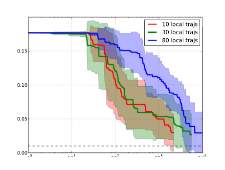
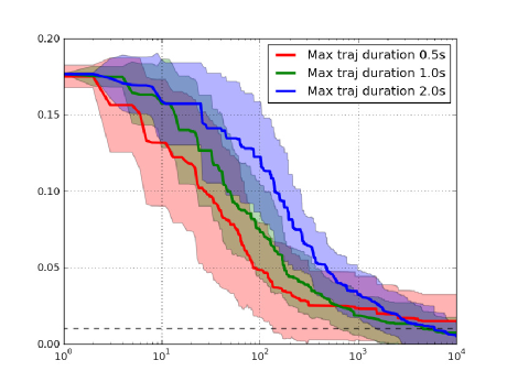
Figure 12: Minimum distance to the goal as a function of time for different values of $N_{\mathrm{local\_trajs}}$ and $\Delta t_{\max}$. At each instant, the minimum distance of the tree to the goal is computed. The average of this value across the 10 trials of each set is drawn in bold, while shaded areas indicate standard deviations. A: tuning of $N_{\mathrm{local\_trajs}}$. B: tuning of $\Delta t_{\max}$.

Fig. 12A shows the result of simulations for different values of $N_{\mathrm{local\_trajs}}$. One can note that the performance of RRT is similar for values $10$ and $30$, but gets worse for $80$. Based on this observation, we chose $N_{\mathrm{local\_trajs}}=20$ for the final comparison in section B.2.

Fig. 12B shows the simulation results for various values of $\Delta t_{\max}$. Observe that the performance of RRT is similar for the three tested values, with smaller values (e.g. 0.5 s) performing better earlier in the trial and larger values (e.g. 2.0 s) performing better later on. We also noted that smaller values of $\Delta t_{\max}$ such as 0.1 s or 0.2 s tended to yield poorer results (not shown here). Our choice for the final comparison was thus $\Delta t_{\max}=1.0$ s.

B.2 Comparing $K$NN-RRT and AVP-RRT

In this section, we compare the performance of $K$NN-RRT (for $K\in\{1,10,40,100\}$, the other parameters being set to the values discussed in the previous section) against AVP-RRT with 10 neighbors. For practical reasons, we further limited the execution time of every trial to $10^{4}$ s, which had no impact in most cases or otherwise induced a slight bias in favor of RRT (since we took $10^{4}$ s as our estimate of the “search time” when RRT does not terminate within this time limit).

We ran the simulations for two instances of the problem, namely

• $(\tau^{\max}_{1},\tau^{\max}_{2})=(11,7)$ N.m;

• $(\tau^{\max}_{1},\tau^{\max}_{2})=(11,5)$ N.m.

For each problem instance, we ran 40 trials for each planner AVP-RRT, state-space RRT with 1 nearest neighbor (RRT-1), RRT-10, RRT-40 and RRT-100. Note that for each trial $i$, all the planners received the same sequence of random states

$$\mathbf{X}_{i}=\left\{\mathbf{x}_{\mathrm{rand}}^{(i)}(t)\in\mathbf{R}^{4}\ \middle|\ t\in\mathbf{N}\right\}\sim{\cal U}\left((]-\pi,\pi]^{2}\times[-V_{\max},+V_{\max}]^{2})^{\mathbf{N}}\right),$$

although AVP-RRT only used the first two coordinates of each sample since it plans in the configuration space. The results of this benchmark were already illustrated in Fig. 7. Additional details are provided in Tables 4 and 5. All trials of AVP successfully terminated within the time limit.

For $(\tau^{\max}_{1},\tau^{\max}_{2})=(11,7)$, the average search time was $3.3$ min. Among the $K$NN-RRT, RRT-40 performed best with a success rate of 92.5% and an average computation time ca. 45 min, which is however $13.4$ times slower than AVP-RRT.

For $(\tau^{\max}_{1},\tau^{\max}_{2})=(11,7)$, the average search time was $9.8$ min. Among the $K$NN-RRT, again RRT-40 performed best in terms of search time (54.6 min on average, which was $5.6$ times slower than AVP-RRT), but RRT-100 performed best in terms of success rate within the $10^{4}$s time limit (92.5%).

Planner	Success rate	Search time (min)
AVP-RRT	100%	3.3$\pm$2.6
RRT-1	40%	70.0$\pm$34.1
RRT-10	82.5%	53.1$\pm$59.5
RRT-40	92.5%	44.6$\pm$42.6
RRT-100	82.5%	88.4$\pm$54.0

Table 4: Comparison of AVP-RRT and $K$NN-RRT for $(\tau^{\max}_{1},\tau^{\max}_{2})=(11,7)$.

Planner	Success rate	Search time (min)
AVP-RRT	100%	9.8$\pm$12.1
RRT-1	47.5%	63.8$\pm$36.6
RRT-10	85%	56.3$\pm$60.1
RRT-40	87.5%	54.6$\pm$52.2
RRT-100	92.5%	81.2$\pm$46.7

Table 5: Comparison of AVP-RRT and $K$NN-RRT for $(\tau^{\max}_{1},\tau^{\max}_{2})=(11,5)$.

Appendix C Comparison of AVP-RRT with KPIECE on a 6-DOF and a 12-DOF manipulators

Here, we detail the comparison between AVP-RRT and the OMPL implementation of KPIECE (Sucan and Kavraki, 2012; Sucan et al., 2012) on a kinodynamic problem involving a $n$-DOF manipulators, for $2\leq n\leq 12$. The full source code for this comparison is available at https://github.com/quangounet/kpiece-comparison.

C.1 KPIECE

We used the implementation of KPIECE available in the Open Motion Planning Library (OMPL) (Sucan et al., 2012). The library provides utilities such as function templates, data structures, and generic implementations of various planners, written in C++ with Python interfaces. It, however, does not provide modules such as collision checker and modules for visualization purposes. Therefore, we used OpenRAVE (Diankov, 2010) for collision checking and visualization.

C.1.1 Overall algorithm

KPIECE grows a tree of motions in the state-space. A motion $\nu$ is a tuple $(s,u,t)$, where $s$ is the initial state of the motion, $u$ is the control being applied to $s$, and $t$ is the control duration. Initially the tree contains only one motion $\nu_{\mathrm{start}}$. Then in each iteration the algorithm proceeds by first selecting a motion on the tree to expand from. A control input is then selected and applied to the state for a time duration. Finally, the algorithm will evaluate the progress that has been made so far.

To select an existing motion from the tree, KPIECE utilizes information obtained from projecting states in the state-space $\mathcal{Q}$ into some low-dimensional Euclidean space $\mathbf{R}^{k}$. Low-dimensionality of the space allows the planner to discretize the space into cells. KPIECE will then score each cell based on several criteria (see (Sucan and Kavraki, 2012) for more detail). Based on an assumption that the coverage of the low-dimensional Euclidean space can reflect the true coverage of the state-space, KPIECE uses its cell scoring system to help bias the exploration towards unexplored area.

For the following simulations, we used KPIECE planner implementation in C++ provided via the OMPL library. Since the library only provides generic implementation of the planner, we also needed to implement some problem specific functions for the planner such as state projection and state propagation. Those functions were also implemented in C++. We will give details on state projection and state propagation rules we used in our simulations.

State projection

Since the state-space exploration is mainly guided by the projection (as well as their cell scoring), more meaningful projections which better reflect the progress of the planner will help improve its performance. For planning problems for a robot manipulator, we used a projection that projects a state to an end-effector position in $3$D space. Sucan and Kavraki (2012) suggested that when planning for a manipulator motion, the tool-tip position in $3$D space is representative. However, by simply discarding all the velocity components we may lose information which can essentially help solve the problem. Thus, we decided to include also the norm of velocity into the projection. This inclusion of the norm of velocity was also used in (Sucan and Kavraki, 2012) when planning for a modular robot. Therefore, the projection projects a state into a space of dimension $4$.

State propagation

KPIECE uses a control-based steering method. It applies a selected control to a state over a number of propagation steps to reach a new state. In our cases, since the robot we were using was position-controlled, our control input were joint accelerations. Let the state be $(\bf{q},\dot{\bf{q}})$, where $\mathbf{q}$ and $\dot{\mathbf{q}}$ are the joint values and velocities, respectively. The new state $(\mathbf{q}^{+},\dot{\mathbf{q}}^{+})$ resulting from applying a control $\ddot{\mathbf{q}}$ to $(\bf{q},\dot{\bf{q}})$ over a short time interval $\Delta t$ can be computed from

$$\mathbf{q}^{+} =\mathbf{q}+\Delta t\dot{\mathbf{q}}+0.5(\Delta t)^{2}\ddot{\mathbf{q}}$$ (14)

$$\dot{\mathbf{q}}^{+} =\dot{\mathbf{q}}+\Delta t\ddot{\mathbf{q}}.$$ (15)

C.1.2 Fine-tuning of KPIECE

We employed $L_{2}$ norm as a distance metric in order not to bias the planning towards any heuristics. Next, in order for the planner not to spend too much running time into simulations for fine-tuning, we selected the threshold value to be $0.1$. The threshold is used to decide whether a state has reached the goal or not. If the distance from a state to the goal, according to the given distance metric, is less than the selected threshold, the problem is considered as solved. Then we tested the algorithm with a number of sets of parameters to find the best set of parameters.

At this stage, the testing environment consisted only of the models of the Denso VS-$060$ manipulator and its base. There was no other object in the environment. Here, to check validity of a state, we need to check for only robot self-collision. In the following runs, we planned motions for only the first two joints of the robot (the ones closest to the robot base). The robot had to move from $(0,0,0,0)$ to $(1,1,0,0)$, where the first two components of the tuples are joint values and the others are joint velocities. We set the goal bias to $0.2$. With chosen parameters and projection, we ran simulations with difference combinations of cell size, $c$, and propagation step size, $p$. Note that here we assigned cell size, which defines the resolution of discretization of the projecting space, to be equal in every dimension. Both cell size and propagation step size were chosen from a set $\{0.01,0.05,0.1,0.5,1.0\}$. We tested for all different $25$ combinations of the parameters and recorded the running time of the planner. We ran $50$ simulations for each pair $(c,p)$. For any value of cell size, we noticed that the propagation step size of $0.05$ performed best. For $p=0.05$, the values $c$ being $0.05,0.1,1.0$ performed better than the rest. The resulting running times using those values of cell size did not significantly differ from each other. The differences were in order of $1$ ms. Therefore, in the following section, we repeated all the simulations with three different pairs $(c,p)\in\{(0.05,0.05),(0.1,0.05),(1.0,0.05)\}$.

C.2 KPIECE simulation results and comparison with AVP-RRT

With the previously selected parameters, we conducted simulations as follows. First of all, to show how running time of KPIECE and AVP-RRT scale when the dimensionality of the problem increases, we used both planners to plan motions for a $n-DOF$ robot, with $2\leq n\leq 12$. For this, we concatenated two Denso VS-$060$ manipulator manipulators together into a composite 12-DOF manipulator and used the first $n$ joints of that robot.

The robot was to move from all-zeros configuration to all-ones configuration. Initial and final velocities were set to zero. There was no other obstacle in the scene. Since the implementation of KPIECE is unidirectional, we also used a unidirectional version of AVP-RRT. The AVP-RRT implementation was written in Python. Only the time-parameterization algorithm was implemented in C++.

We gave each planner 200 s. for each run, and simulated $20$ runs for each condition. For KPIECE we tested different values of cell sizes (0.05, 0.1, and 1.0). Fig. 13A shows average running times over 20 runs. From the figure, the three values of the cell size produced similar results. Although KPIECE performed well when planning for low numbers of DOFs, the running time increased very quickly (exponentially) with increasing numbers of DOFs. Correlatively, the success rate when planning using KPIECE dropped rapidly when the number of DOFs increased, as can be seen from Fig. 13A. When the number of DOFs was higher than 8, KPIECE failed to find any solution within 200 s. The computation time for AVP-RRT also increased exponentially with the number of DOFs but the rate was much lower as compared to KPIECE.

A                                           B

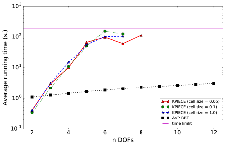
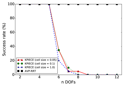
Figure 13: A : Average running time of KPIECE and AVP-RRT (black squares) taken over $20$ runs as a function of the number of DOF. For KPIECE, simulations were run with three different cell sizes: $0.05$ (red triangles), $0.1$ (green circles), and $1.0$ (blue stars). B : Succcess rates of KPIECE and AVP-RRT over $20$ runs. When the number of DOFs was higher than 8, KPIECE failed to find any solution within the given time limit of 200 s.

Finally, we considered an environment similar to that of our experiment on non-prehensile object transportation of Section 4.2. The tray and the bottle were, however, removed from the (6-DOF) robot model. The problem was therefore less constrained. We considered here only bounds on joint values, joint velocities, and joint accelerations. We shifted the lower edge of the opening upward for $13$ cm. and set the opening height to be lower ($25$ cm. in this case) to make the problem more interesting. Then for each run, both planners had a time limit of $600$ s to find a motion for the robot to move from one side of the wall to the other. We repeated simulations $20$ times for both planners. For KPIECE, since the performance when using different cell size from $\{0.05,0.1,1.0\}$ did not differ much from each other, we chose to ran simulations with cell size $c=0.05$.

The average running time for AVP-RRT in this case was $68.67$ s with a success rate of $100\%$. The average number of nodes in the tree when the planner terminated was $60.15$ and the average number of trajectory segments of the solutions was $8.60$. Fig. 14 shows the scene used in simulations as well as an example of a solution trajectory found by AVP-RRT. On the other hand, KPIECE could not find any solution, in any run, within the given time limit.

A                                                            B

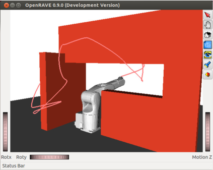
Figure 14: The scene used in the last experiment. Both KPIECE and AVP-RRT were to find a motion for the robot to move from one side of the wall to the other. A: the start configuration of the robot. B: the goal configuration of the robot. The pink line in the figure indicates an end-effector path from a solution found by AVP-RRT. KPIECE could not find any solution, in any run, within the given time limit of 600 s.

References

- Bobrow [1988] J.E. Bobrow. Optimal robot path planning using the minimum-time criterion. IEEE Journal of Robotics and Automation, 4(4):443–450, 1988.
- Bobrow et al. [1985] J.E. Bobrow, S. Dubowsky, and JS Gibson. Time-optimal control of robotic manipulators along specified paths. The International Journal of Robotics Research, 4(3):3–17, 1985.
- Bullo and Lynch [2001] F. Bullo and K. M. Lynch. Kinematic controllability for decoupled trajectory planning in underactuated mechanical systems. IEEE Transactions on Robotics and Automation, 17(4):402–412, 2001.
- Caron et al. [2014] S. Caron, Q.-C. Pham, and Y. Nakamura. Completeness of randomized kinodynamic planners with state-based steering. In Proceedings of the International Conference on Robotics and Automation, pages 5818–5823, 2014.
- Diankov [2010] R. Diankov. Automated Construction of Robotic Manipulation Programs. PhD thesis, Carnegie Mellon University, Robotics Institute, August 2010. URL http://www.programmingvision.com/rosen_diankov_thesis.pdf.
- Donald et al. [1993] B. Donald, P. Xavier, J. Canny, and J. Reif. Kinodynamic motion planning. Journal of the ACM (JACM), 40(5):1048–1066, 1993.
- Escande et al. [2013] A. Escande, A. Kheddar, and S. Miossec. Planning contact points for humanoid robots. Robotics and Autonomous Systems, 61(5):428–442, 2013.
- Geraerts and Overmars [2007] R. Geraerts and M.H. Overmars. Creating high-quality paths for motion planning. The International Journal of Robotics Research, 26(8):845–863, 2007.
- Hauser [2014] K. Hauser. Fast interpolation and time-optimization with contact. The International Journal of Robotics Research, 33(9):1231–1250, 2014.
- Hauser et al. [2008] K. Hauser, T. Bretl, J.-C. Latombe, K. Harada, and B. Wilcox. Motion planning for legged robots on varied terrain. The International Journal of Robotics Research, 27(11-12):1325–1349, 2008.
- Hsu et al. [2002] D. Hsu, R. Kindel, J.-C. Latombe, and S. Rock. Randomized kinodynamic motion planning with moving obstacles. The International Journal of Robotics Research, 21(3):233–255, 2002.
- Hsu et al. [2003] D. Hsu, T. Jiang, J. Reif, and Z. Sun. The bridge test for sampling narrow passages with probabilistic roadmap planners. In Robotics and Automation, 2003. Proceedings. ICRA’03. IEEE International Conference on, volume 3, pages 4420–4426. IEEE, 2003.
- Johnson and Hauser [2012] J. Johnson and K. Hauser. Optimal acceleration-bounded trajectory planning in dynamic environments along a specified path. In IEEE International Conference on Robotics and Automation, pages 2035–2041, 2012.
- Kalakrishnan et al. [2011] M. Kalakrishnan, S. Chitta, E. Theodorou, P. Pastor, and S. Schaal. Stomp: Stochastic trajectory optimization for motion planning. In IEEE International Conference on Robotics and Automation, pages 4569–4574, 2011.
- Kant and Zucker [1986] K. Kant and S. W. Zucker. Toward efficient trajectory planning: The path-velocity decomposition. The International Journal of Robotics Research, 5(3):72–89, 1986.
- Karaman and Frazzoli [2011] Sertac Karaman and Emilio Frazzoli. Sampling-based algorithms for optimal motion planning. The International Journal of Robotics Research, 30(7):846–894, 2011.
- Kavraki et al. [1996] L.E. Kavraki, P. Svestka, J.C. Latombe, and M.H. Overmars. Probabilistic roadmaps for path planning in high-dimensional configuration spaces. Robotics and Automation, IEEE Transactions on, 12(4):566–580, 1996.