Measure of combined effects of morphological parameters of inclusions within composite materials via stochastic homogenization to determine effective mechanical properties

Abstract

In our previous papers we have described efficient and reliable methods of generation of representative volume elements (RVE) perfectly suitable for analysis of composite materials via stochastic homogenization.

In this paper we profit from these methods to analyze the influence of the morphology on the effective mechanical properties of the samples. More precisely, we study the dependence of main mechanical characteristics of a composite medium on various parameters of the mixture of inclusions composed of spheres and cylinders. On top of that we introduce various imperfections to inclusions and observe the evolution of effective properties related to that.

The main computational approach used throughout the work is the FFT-based homogenization technique, validated however by comparison with the direct finite elements method. We give details on the features of the method and the validation campaign as well.

I Introduction / motivation

In this paper we study the influence of morphological parameters of composite materials on their effective mechanical properties. The usage of composite materials for industrial applications motivated a huge amount of publications on the subject in recent years: they concern both experimental and modelling results. The reason for us to address the question is twofold as well: on the one hand we explore the existing modelling techniques, on the other hand we have in mind very concrete applications related to the project in the industry of aeronautics.

The need in modelling for the analysis of composite materials as in most of the applied domains comes from the fact that experimental work is usually expensive and difficult to carry out. It is thus important to develop modelling approaches that are efficient, reliable and sufficiently flexible so that the outcome can be validated by an experiment. The strategy that we adopt here is related to the notions of stochastic homogenization. The key idea is to consider a sample of a composite material that is sufficiently large to capture its behavior and compute the macroscopic parameters: for mechanical properties it can be for example the Young modulus, the Poisson ratio or eventually the whole stiffness tensor. To take into account possible imperfections or random factors one can average the result for a series of tests representing the same macro characteristics. The usual technology for this is to generate a series of samples (representative volume elements) randomly, controlling though their parameters, perform the computation for each of them and average the result.

It is now generally accepted that the main characteristic affecting the effective properties of a composite material is its morphology, i.e. the combination of geometric characteristics of the inclusions and their distribution in the supporting matrix. To analyze the phenomenon one needs thus a tool to generate RVEs capturing various morphological parameters. We have developed and implemented such a tool: in VDP we described the algorithms to produce the RVEs containing spheres (that represent globular inclusions) and cylinders (that are responsible for fiber-type reinforcements). We are able to reach the volume fraction of inclusions up to relatively high values of 50%–60%, and in addition we can control the geometric configuration of a sample as a whole, namely manage the intersections of inclusions and eventually their distribution. Moreover in SVDP we have extended the method to introduce irregularities to the shape of inclusions. In this paper we describe the results of computations carried out with the generated samples via an FFT-based homogenization technique (moul-suq ; monchiet ). For the presentation here we have chosen the results that can be useful for applications and/or those where the trends are not intuitively obvious, in particular we explore the influence of redistribution of the volume fraction between globular and fiber-type reinforcements, as well as the effects of imperfections.

The paper is organized as follows. In the next section we briefly recall the RVE generation methods proposed in VDP and extended in our further works. In its second part we give details about the main computational method which is used throughout the work: the FFT-based homogenization technique coupled with stochastic methods of RVE generation. We describe its convenience and limitations as well as present the results of the validation campaign, i.e. compare it with the direct finite elements method. The section III is the description of the results of analysis (via the above mentioned methods) of effective properties of composites depending on the morphological parameters of the inclusions. We conclude by describing eventual industrial applications, some work in progress and expected results of it.

II Sample generation and computational techniques

As we have outlined in the introduction, this section is devoted to a brief description of the methods that we have used to perform computations and the reasons to choose these concrete methods.

II.1 RVE generation

The generation of samples for computation is an important step in the process of modelling of the behavior of composite materials. Since the morphology of composites may be quite complex this can be a very challenging task. On the one hand it is important to be able to approximate rather involved geometries, on the other hand the method should be fast and reliable; in the ideal case the stage of generation should be much shorter than the computation itself.

There has been a number of works where the inclusions were represented by simple geometric objects like spheres or ellipsoids (see for example, segu ; levesque_sp ; zhao ; man ). If one considers more complicated geometry, the problem of managing the intersection of inclusions arises immediately. Among the established approaches of dealing with it, one can mention two important families: random sequential adsorption (RSA) type algorithms and molecular dynamics (MD) based methods. The RSA (rsa1 ) is based on sequential addition of inclusions verifying for each of them the intersection; the main idea of the MD (LSA ; williams ; levesque_ell ) is to make the inclusions move, until they reach the desired configuration. Let us mention that the first method needs an efficient algorithm of verification of intersection between the geometric shapes, and the second one an algorithm of predicting the time to the intersection of moving objects, which exists for a very limited class of shapes and often amounts to a difficult minimization problem. In VDP , we have described the classical RSA and a time-driven version of MD applied to the mixture of inclusions of spherical and cylindrical shapes. The key ingredient for both of the approaches was the explicit formulation of algebraic conditions of intersection of a cylinder with a sphere and of two cylinders. To be more specific, we recapitulate the ideas of these algorithms (Algorithms 1, 2).

We have observed that the RSA approach is extremely efficient for relatively small volume fractions of inclusions (up to $30\%$), where it permits to generate a sample in fractions of a second. The MD-based method is powerful for higher volume fractions (of order $50-60\%$): it generates a configuration in about a second while the RSA can get stuck. An example of a sample with a mixture of non-intersecting spherical and cylindrical inclusions is presented on the figure 1.

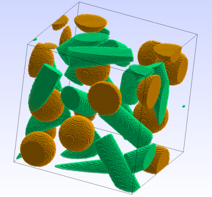
Figure 1: 3D view of an RVE: spherical and cylindrical inclusions, periodic boundary conditions.

Algorithm 1

RSA generation procedure.
Input: volume fractions, number of inclusions $n_{cyl},n_{sp}$, aspect ratio.
1. Compute the parameters of cylinders and spheres 2. NumOfGenSpheres = 0, NumOfGenCylinders = 0 3. while $(NumOfGenCylinders<n_{cyl})$
(a) Generate a new cylinder (b) Using the algorithm (VDP , Alg. 4) check if it overlaps with any cylinder generated before (c) if yes redo 3a (d) if no increase NumOfGenCylinders 4. while $(NumOfGenSpheres<n_{sp})$
(a) Generate a new sphere (b) Check if it overlaps with any sphere generated before (c) if yes redo 4a (d) Using the algorithm (VDP , Alg. 1) check if it overlaps with any cylinder generated before (e) if yes redo 4a (f) if no increase NumOfGenSpheres

Algorithm 2

MD-based generation procedure.
Input: volume fractions, number of inclusions $n_{cyl},n_{sp}$, aspect ratio.
1. Compute the parameters of cylinders and spheres, fix the criterion $\varepsilon$ to stop the simulation 2. Generate $n_{sp}$ spheres and $n_{cyl}$ cylinders, disregarding overlapping 3. while (OverlappingEnergy $>\varepsilon$)
(a) Check overlapping (VDP , Alg. 1, 4) (b) For each couple of overlapping inclusions compute the interaction force (VDP , table 1) (c) Perform the integration step for the evolution equations (VDP , Eq. 6) (d) Update the value of OverlappingEnergy

The outcome of these algorithms is a list of inclusions in the “vector” form, i.e. a list of coordinates of centers, radii, and eventually axes of symmetry of inclusions. This is perfectly suitable for various computational techniques: FFT-based homogenization procedures applied to the pixelized samples, as well as finite element computations on the mesh constructed from this pixelization. In addition (SVDP ) we are able to introduce various imperfections of the inclusions without spoiling the efficiency of the generation algorithm: the figure 2 shows two such examples, where the surface of an inclusion is waved or a part of an inclusion is taken out to produce irregular shapes.

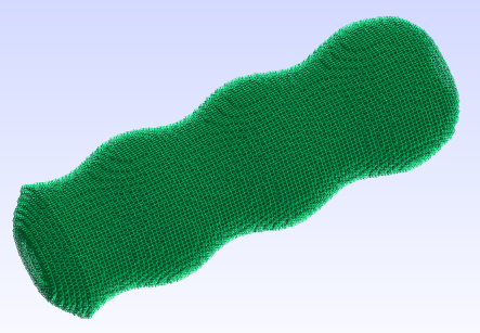
(a)   Waved surface of an inclusion

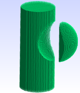
(b)   Part of an inclusion taken out

Figure 2: Various imperfections of inclusions.

II.2 FFT-based homogenization scheme

Having an efficient scheme of generation of samples we can now proceed to the computation of effective mechanical properties. As we have mentioned in the introduction for evaluating these properties we have adopted the philosophy of stochastic homogenization. Schematically one can view the process as follows:

1. Fix the macroscopic parameters of the material (volume fraction and type of inclusions).

2. Generate a series of samples (RVEs) of a composite material with these parameters
   (stochastic part).

3. Perform accurate computation of effective properties on these RVEs
   (deterministic homogenization part).

4. Average the computed (macroscopic) characteristics of the samples.

Let us now describe the mechanical model behind this computation as well as the main computational method – the homogenization procedure.

Consider a representative volume element $V$, and denote $\mathbf{u}(\mathbf{x})$ the displacement field defined at any point $\mathbf{x}\in V$. The system in mechanical equilibrium is described by the law $\sigma(\mathbf{x})=\frac{\partial w(\mathbf{x})}{\partial\varepsilon(\mathbf{x})}$, where $\varepsilon(\mathbf{x})=\varepsilon(\mathbf{u}(\mathbf{x}))=\frac{1}{2}(\nabla\mathbf{u}(\mathbf{x})+\nabla\mathbf{u}(\mathbf{x})^{T})$ – the strain tensor in the model of small deformations, $w(\mathbf{x})$ – the stored mechanical energy, and $\sigma(\mathbf{x})$ – the stress tensor, subject to the condition $\mathrm{div}\,\sigma(\mathbf{x})=0$. In the linear case this law simplifies to $\frac{\partial w(\mathbf{x})}{\partial\varepsilon(\mathbf{x})}=c(\mathbf{x})\!:\!\varepsilon(\mathbf{x})$ with the stiffness tensor $c(\mathbf{x})$. Notice that for a composite material the stiffness tensor does depend on the point $\mathbf{x}$: the dependence is governed by microscopic geometry of the sample, namely which phase (matrix or inclusion) the point $\mathbf{x}$ belongs to. We suppose that the averaged strain $<\!\varepsilon\!>=E$ is prescribed, and decompose $\varepsilon(\mathbf{x})$ in two parts: $\varepsilon(\mathbf{u}(\mathbf{x}))=E+\varepsilon(\mathbf{\tilde{u}}(\mathbf{x}))$, which is equivalent to representing $\mathbf{u}(\mathbf{x})=E.\mathbf{x}+\mathbf{\tilde{u}}(\mathbf{x})$, for $\mathbf{\tilde{u}}(\mathbf{x})$ being periodic on the boundary of $V$. Thus, the problem we are actually solving reads

$$\sigma(\mathbf{x})=c(\mathbf{x}):(E+\varepsilon(\mathbf{\tilde{u}}(\mathbf{x})),\quad\mathrm{div}\,\sigma(\mathbf{x})=0,$$ (1)

$$\mathbf{\tilde{u}}(\mathbf{x})\,\,\mathrm{periodic},\,{\sigma}(\mathbf{x}).\mathbf{n}\,\,\mathrm{antiperiodic}.$$

The solution of (1) is the tensor field $\sigma(\mathbf{x})$, we are interested in its average in order to obtain the homogenized stiffness tensor $c_{hom}$ from the equation

$$<\!\sigma(\mathbf{x})\!>=c_{hom}:<\!\varepsilon(\mathbf{x})\!>.$$ (2)

To recover all the components of $c_{hom}$ in 3-dimensional space one needs to perform the computation of $<\!\sigma(\mathbf{x})\!>$ for six independent deformations $E$, which morally correspond to usual stretch and shear tests.

There is a couple of natural approaches to solving the problem (1): one can construct a mesh of an RVE $V$ and employ the finite elements method, or discretize (basically pixelize) the RVE to use the FFT-based homogenization scheme (moul-suq ; monchiet ). The major difficulty arising when applying the former method is that for rather involved geometry one needs to construct a fine mesh which is a non-trivial task in its own, and moreover to proceed with finite elements one requires considerable memory resources. The idea of the latter is that in the Fourier space the equations of (1) acquire a rather nice form for which in the case of a homogeneous isotropic material one can construct a Green operator and basically produce an exact solution. For a composite material containing possibly several phases one introduces an artificial reference medium for which the Green operator is defined, the computation then is an iterative procedure to approximate the corrections of the microscopic behavior of the material in comparison to this reference medium. For the sake of completeness let us present this method here in details, following essentially the works MMS ; eyre .

Introduce the reference medium stiffness tensor $c^{0}$ and the correction to it
$\delta c(\mathbf{x})=c(\mathbf{x})-c^{0}$. The equations (1) can equivalently be rewritten as

$$\sigma(\mathbf{x})=c^{0}:\varepsilon(\mathbf{\tilde{u}}(\mathbf{x}))+\tau(\mathbf{x}),\quad\mathrm{div}\,\sigma(\mathbf{x})=0,$$ (3)

$$\tau(\mathbf{x})=\delta c(\mathbf{x}):(\varepsilon(\mathbf{\tilde{u}}(\mathbf{x}))+E)+c^{0}:E,$$

$$\mathbf{\tilde{u}}(\mathbf{x})\,\,\mathrm{periodic},\,{\sigma}(\mathbf{x}).\mathbf{n}\,\,\mathrm{antiperiodic}.$$

The tensor $\tau$ is called polarization. The periodicity assumptions permit to rewrite the first line of (3) in the Fourier space. Using the linearity of the Fourier transform and its property with respect to derivation, one obtains

$$\hat{\sigma}_{mj}(\mathbf{\xi})=ic^{0}_{mjkl}\xi_{l}\hat{\tilde{u}}_{k}(\mathbf{\xi})+\hat{\tau}_{mj}(\mathbf{\xi}),\quad i\hat{\sigma}_{mj}\xi_{j}=0,$$

where $\hat{\bullet}$ denotes the Fourier image of $\bullet$ and $\xi_{j}$’s are the coordinates in the Fourier space. The key observation is that in the Fourier space there is a relation between the polarization and the deformation tensors, namely
$\hat{\tilde{\varepsilon}}(\mathbf{\xi})=-\hat{\Gamma}^{0}(\mathbf{\xi}):\hat{\tau}(\mathbf{\xi})$. $\Gamma^{0}$ is the Green operator, which for an isotropic reference medium with the Lamé coefficients $\lambda_{0},\mu_{0}$ can be computed explicitly:

$$\hat{\Gamma}^{0}_{klmj}(\mathbf{\xi})=\frac{\displaystyle\delta_{km}\xi_{l}\xi_{j}+\delta_{lm}\xi_{k}\xi_{j}+\delta_{kj}\xi_{l}\xi_{m}+\delta_{lj}\xi_{k}\xi_{m}}{\displaystyle 4\mu_{0}|\mathbf{\xi}|^{2}}-\frac{\displaystyle\lambda_{0}+\mu_{0}}{\displaystyle\mu_{0}(\lambda_{0}+2\mu_{0})}\frac{\displaystyle\xi_{j}\xi_{k}\xi_{l}\xi_{m}}{\displaystyle|\mathbf{\xi}|^{4}}$$

Going back to the original variables, the initial problem (3) reduces to the periodic Lippmann–Schwinger integral equation

$$\varepsilon(\mathbf{u}(\mathbf{x}))=-\Gamma^{0}(\delta c:\varepsilon(\mathbf{u}(\mathbf{x})))+E,$$

This equation can be solved iteratively using the following algorithm.

Algorithm 3

FFT-based numerical scheme.
Initialize $\varepsilon^{0}(\mathbf{x})\equiv E$, fix the convergence criterion $acc$.
while (not converged)
1. Convergence test:
if $(\epsilon_{comp}<acc)$ compute $\sigma(\mathbf{x})=c(\mathbf{x}):\varepsilon^{n}(\mathbf{x})$, $\hat{\sigma}(\mathbf{\xi})=FFT(\sigma)$,
$\epsilon_{eq}=\sqrt{<\!\|\mathbf{\xi}\hat{\sigma}(\mathbf{\xi})^{n}\|^{2}\!>}/\|\hat{\sigma}(0)\|$
if $(\epsilon_{eq}<acc)\rightarrow converged,stop$ 2. $\tau^{n}(\mathbf{x})=(c(\mathbf{x})+c^{0}):\varepsilon^{n}(\mathbf{x})$ 3. $\hat{\tau}^{n}(\mathbf{\xi})=FFT(\tau^{n})$ 4. $\hat{\varepsilon}^{n}_{comp}(\mathbf{\xi})=\hat{\Gamma}^{0}(\mathbf{\xi}):\hat{\tau}^{n}(\mathbf{\xi})$, $\mathbf{\xi}\neq 0$;     $\hat{\varepsilon}^{n}_{comp}(0)=E$ 5. $\varepsilon^{n}_{comp}(\mathbf{x})=FFT^{-1}(\hat{\varepsilon}^{n}_{comp})$ 6. $\epsilon_{comp}=\sqrt{<\!\|\varepsilon^{n}-\varepsilon^{n}_{comp}\|^{2}\!>}/\|E\|$ 7. $\varepsilon^{n+1}(\mathbf{x})=\varepsilon^{n}(\mathbf{x})-2(c(\mathbf{x})-c^{0})^{-1}:c^{0}:(\varepsilon^{n}_{comp}(\mathbf{x})-\varepsilon^{n}(\mathbf{x}))$

When the above algorithm converges we can compute $<\!\sigma(\mathbf{x})\!>$ to be inserted into the equation (2). As we have mentioned above this computation has to be repeated for a complete set of independent global deformation fields.

We have chosen this approach for its computational efficiency both in time and memory consumption, and also for its convenience in the applied problems, that we will discuss afterwards. There are however some details worth being commented on here.

First, there are several versions of such FFT-based schemes: there is a possibility to use the initial variables $\sigma$ and $\varepsilon$ or formulate a dual problem the solution of which will produce the compliance tensor. One can produce a sort of mixture of the two, using polarization as the primary variable. The efficiency of these methods depends on the contrast between the characteristics of different phases. We have chosen to implement the direct accelerated scheme presented above, since there one has a theoretical result on the optimal values of parameters of the reference medium. According to the convergence theorem formulated in eyre , for a two-phase composite with the Lamé coefficients of the constituent phases $(\lambda_{1},\mu_{1})$ and $(\lambda_{2},\mu_{2})$ respectively, one should choose $\lambda_{0}=-\sqrt{\lambda_{1}\lambda_{2}}$, $\mu_{0}=-\sqrt{\mu_{1}\mu_{2}}$ to compute $c^{0}$. The optimality of this accelerated scheme is also coherent with recent results of 2014 .

Second, we have carried out a validation campaign by comparing the results of computations using the FFT-based process, several types of finite elements approaches, and analytical results where possible. We have constructed some test samples with simple geometries: a square bar with different orientations, a plane cutting the sample in two parts, etc. In addition to the FFT-based scheme for these samples we have computed the stiffness tensor using finite elements with the adapted mesh and with the mesh constructed from the pixelized sample. In both cases we used about $2^{18}$ hexahedron elements : parallelepipeds for the adapted mesh constructed with Cast3M, and cubes corresponding to voxels for the mesh built from pixelized sample. The computation with adapted meshes gives results which are in good agreement with theoretical estimations, while with the mesh obtained from the pixelization there is a tendency of overestimating the parameters (when the inclusions are more rigid than the matrix). Although for the values of contrast between the matrix and the inclusions that interest us the difference can reach $1-2\%$, which is not of great importance for observing the trends. What is more interesting is that the FFT-based scheme produces the results where the parameters are often underestimated (up to $5\%$). The situation is certainly reversed when the inclusions are less rigid than the matrix. For computing mechanical properties of composite materials a simple way out is to increase the resolution of pixelization. For the tests that we describe in this paper the pixelization at around $200\times 200\times 200$ already produces reasonable results. For each given sample like the one presented at figure 1 it is sufficient to make several tests at different resolutions for the same vector data and observe when the result stabilizes. Let us however note that if one is interested in thermal properties, where typically there are more than two phases with rather fine geometry, the problem can be much more complicated – we will suggest some more advanced techniques of adapting a sample to such computations elsewhere.

Third, as mentioned the stochastic part of computations is due to averaging the results for several samples with the same macroscopic characteristics. This is the usual approach inspired by the Monte Carlo method. Since the pioneer work monte-carlo of Metropolis and Ulam, there has been a great number of applications of this method for various problems in pure mathematics (VS ), physics (kats ), engineering (mc-eng ; levesque_ell ; Leclerc2012 ; Leclerc2013b ; Leclerc2013c ), science in general. In the concrete context of homogenization and estimation of effective properties of composite materials a natural problem arises: having computed the average for a given sampling we need to decide how far it is from the real average. The usual way to do it is to use Student’s distribution to compute the confidence intervals from the sampling mean value and the standard deviation (see for example levesque_sp ) for a precise algorithm. In our tests it was sufficient to make $10-20$ runs to obtain acceptably small values of deviation, and $20$ was needed not very often – mostly for high values of volume fraction of inclusions and significant contrast between the two materials. We do not depict the confidence intervals on the figures that follow not to overload the plots, we however verify for each of them that the trends that we exhibit are not due to statistical errors.

III Mechanical properties of composites

In this section we present the tendencies of the behaviour of composite materials for various morphological parameters, that we have obtained by making a series of tests using the algorithms described above. We start with simple tests, the aim of which is more to validate the methods in the sense that they produce expected results for simple tendencies. We continue with more involved analysis of influence of combinations of morphological parameters.

With the algorithm of generation of RVEs we are able to control a number of parameters. As we have already mentioned we are working with spheres and cylinders that are supposed to represent respectively globular inclusions and microfiber reinforcements. For both types of inclusions we are able to assign the volume fraction in the generated sample: $f_{sp}$ and $f_{cyl}$ respectively. We can choose the number of inclusions for each type ($n_{sp}$, $n_{cyl}$), and for cylinders we have an extra parameter of aspect ratio (the ratio between the length of a cylinder and its diameter). This already gives a lot of parameters, on top of that we will introduce the imperfections to inclusions – we will comment on them at the end of this section. The result certainly depends on the mechanical parameters of the matrix and the inclusions – we describe this concisely by fixing the value of contrast between the two media. The output is thus the normalized (with respect to the matrix) value of homogenized parameters. We have carried out several series of computations varying these parameters, in this paper we present a selection of results that are qualitatively not obvious from the first sight or quantitatively important for applications.

III.1 Basic tests

Before starting the real computations we need to fix one more detail, namely the typical size of the representative volume element. According to kanit the size is acceptable if increasing it does not modify the result of computations. In our case fixing the relative size of an RVE is equivalent to determine the minimal acceptable number of inclusions. A small number of inclusions clearly corresponds to a small piece of material studied, while the large number means that each sample includes sufficient microscopic variety and is close to being homogeneous in the context of effective properties. We have analyzed the dependence of effective properties on the number of inclusions with all the other parameters being fixed. The typical trend is shown on the figure 3, which clearly shows that from the total number of $20$ the properties stabilize, the effect is more pronounced for higher volume fractions. In all the computations that follow, we will thus consider the number of inclusions of this order.

Figure 3: The dependence of mechanical parameters of a composite on the number of inclusions for the volume fraction being fixed. Contrast 2048.

Let us now turn to analysis of the influence of morphological properties. Here and in what follows we will depict the trends for the effective bulk and shear moduli or for just one of them, since they are usually rather similar qualitatively. In principal we are computing the whole homogenized stiffness tensor, that turns out to be very close to isotropic, it is thus possible to extract any combination of mechanical characteristics out of it (Young modulus, Poisson ratio, Lamé coefficients). The choice of the bulk and the shear moduli is motivated by further comparison with experimental measurements and datasheets.

To start with, let us consider only spherical inclusions (figure 4) and only cylindrical ones (figure 5). For the spheres at contrast greater than $1$ the effective parameters increase non-linearly with the volume fraction, and decrease for the contrast less than $1$. The further the contrast is from $1$ the more this effect is pronounced. The similar effect is observed for the cylinders, and in addition to this the reinforcement by longer inclusions (with higher aspect ratio) is more efficient.

These first tests should be considered more as preparatory results and validation check for the methods, since their outcome is rather predictable. In what follows we discuss more interesting tests.

(a)   Bulk modulus

(b)   Shear modulus

Figure 4: The dependence of mechanical parameters of a composite on the volume fraction of spherical inclusions. $n_{sp}=20$, a similar picture for 15 and 25.

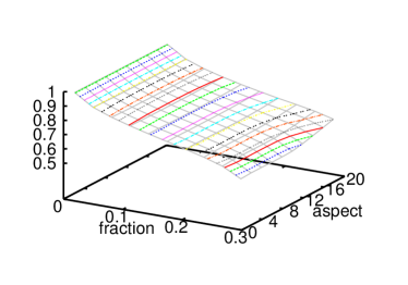
(a)   Contrast 0.0625, normalized bulk modulus

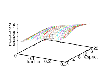
(b)   Contrast 16, normalized bulk modulus

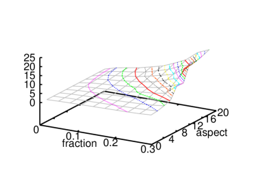
(c)   Contrast 2048, normalized bulk modulus

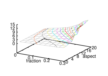
(d)   Contrast 2048, normalized shear modulus

Figure 5: The dependence of mechanical parameters of a composite on the volume fraction and aspect ratio of cylindrical inclusions. $n_{cyl}=20$

III.2 Advanced morphology analysis

Let us now turn to more subtle questions related to analysis of the influence of morphology on the effective properties of composite materials, namely let us consider the composites reinforced by the mixture of globular and fiber-type inclusions and understand what factors in repartition of the inclusions to these two types influence the result.

In the first series of tests here we fix the overall number of inclusions of both type and study the dependence of the effective properties on the aspect ratio of the cylindrical inclusions for various volume fractions. The results (figure 6) clearly show that for contrast greater than $1$ the composite is better reinforced with longer cylinders. The effect is certainly better visible for higher contrast. Although as expected the presence of spherical inclusions in the mixture does not permit to reach the same values of parameters of the homogenized medium as in the case of the same volume fraction formed by cylinders only (cf. figure 5). The opposite effect is present for values of contrast less than $1$, but quantitatively it is less pronounced.

(a)   Contrast 0.0625, normalized bulk modulus

(b)   Contrast 16, normalized bulk modulus

(c)   Contrast 256, normalized bulk modulus

(d)   Contrast 2048, normalized bulk modulus

Figure 6: The dependence of mechanical parameters of a composite material on the aspect ratio of the cylinders in the mixture of inclusions. Comparison for $n_{sp}=n_{cyl}=20$.

Let us now fix the volume fraction of each type of inclusions and vary the number of them. The figure 7 shows that the reinforcement/weakening is slightly more efficient with a large number of cylinders. Although looking at numerical values one sees that the effect is rather subtle and can be neglected in the global analysis. Notice that there is a saturation phenomenon when the total number of inclusions is small, which is in perfect agreement with the above discussion about the size of an RVE and figure 3.

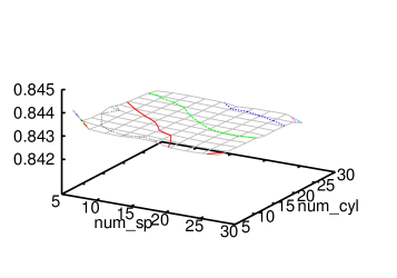
(a)   $f_{sp}\!=\!f_{cyl}=0.05$, contrast 0.0625, normalized bulk modulus

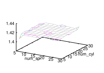
(b)   $f_{sp}=f_{cyl}=0.05$, contrast 2048, normalized bulk modulus

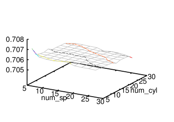
(c)   $f_{sp}=f_{cyl}=0.1$, contrast 0.0625 normalized bulk modulus

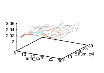
(d)   $f_{sp}=f_{cyl}=0.1$, contrast 2048 normalized bulk modulus

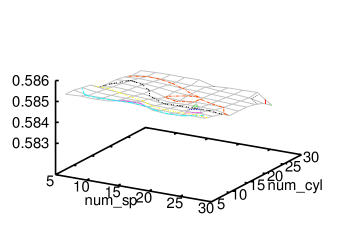
(e)   $f_{sp}=f_{cyl}=0.15$, contrast 0.0625 normalized bulk modulus

(f)   $f_{sp}=f_{cyl}=0.15$, contrast 2048 normalized bulk modulus

Figure 7: The dependence of mechanical parameters of a composite material on the number of various inclusions for fixed volume fraction. Note that the scale on these plots is different from all the others: the difference between the minimal and the maximal values is almost absorbed by the confidence intervals, except the corner with the small number of inclusions (cf. also figure 3).

The most interesting series of tests from this group is the study of the influence of repartition of the volume of inclusions between spheres and cylinders. The diagonals of each plot on the figure 8 represent the volume fractions of two types of inclusions with a fixed sum. One can again notice that the reinforcement/weakening effect is better observed for cylinders than for spheres.

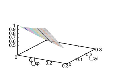
(a)   contrast 0.0625, normalized bulk modulus

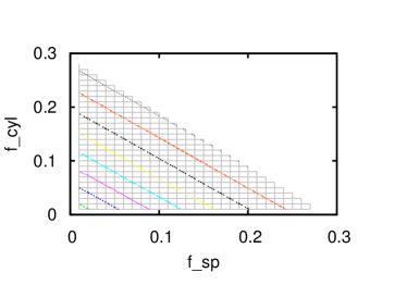
(b)   contrast 0.0625, normalized bulk modulus

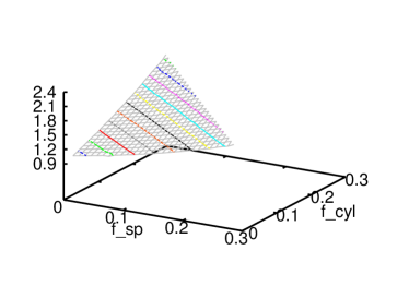
(c)   contrast 16, normalized bulk modulus

(d)   contrast 16, normalized bulk modulus

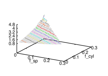
(e)   contrast 2048, normalized bulk modulus

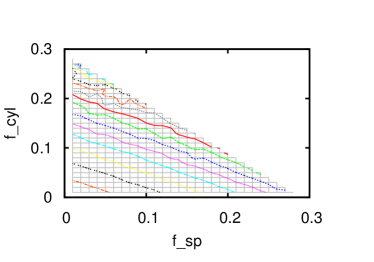
(f)   contrast 2048, normalized bulk modulus

Figure 8: The dependence of mechanical parameters of a composite material on the repartition of inclusions volume between spheres and cylinders. $n_{sp}=n_{cyl}=20$. 3D plot on the left, level sets map on the right.

III.3 Imperfections

The following two series of tests represent the most true to life situations when the inclusions are not of ideal shape. With the algorithms from VDP we are able to generate various types of imperfections including perturbing the surfaces of inclusions by waves and taking out parts of the inclusions preserving the overall volume fraction (figure 2). Let us mention that generating these imperfections we still suppose that the interface between the two materials is perfect, i.e. no voids or discontinuities are created. This proves to be a reasonable assumption for mechanical properties, let us note though that if one studies for example thermal or electrical conductivity the result is more subtle (cf. yvonnet ).

In the first case the main parameter is the relative wave amplitude, i.e. the ratio between the amplitude of perturbations of the surface and some characteristic size of the inclusions (radii of spheres and cylinders in the performed computations). A typical dependence of the effective properties on this parameter for several aspect ratios of cylinders in the mixture is presented on figure 9. The trends observed there leave no doubt that such perturbations in fact contribute to more efficient reinforcement of the material. Our computations show that the effect is more pronounced when the composite is already well reinforced, i.e. at higher volume fraction, larger aspect ratio of cylinders, or significant contrast between two phases.

(a)   aspect 3, normalized bulk modulus

(b)   aspect 6, normalized bulk modulus

(c)   aspect 9, normalized bulk modulus

(d)   aspect 9, normalized shear modulus

Figure 9: The dependence of mechanical parameters of a composite on the waving of the surface of inclusions. $n_{sp}=n_{cyl}=20$, contrast 2048.

The second series of tests concerns the simulation of possible defects while introducing the inclusions to the matrix of the future composite material. We model this process by generating the zones where the obtained composite is “spoilt”, namely if the inclusion intersects partially with such a zone some piece of it is moved out and placed apart in the matrix. The main parameter of this perturbation is thus the volume fraction of such zones. The figure 10 shows the effect of the amount of defects on the properties of a material. The curves are less smooth than for most of the dependencies presented above, but globally one sees that the defects (at least at reasonable volume fraction) contribute to reinforcement as well. And as before, the more the studied material was reinforced without imperfections, the clearer this effect is visible.

(a)   aspect 3, normalized bulk modulus

(b)   aspect 6, normalized bulk modulus

(c)   aspect 9, normalized bulk modulus

(d)   aspect 9, normalized shear modulus

Figure 10: The dependence of mechanical parameters of a composite on the volume of defects in the material. $n_{sp}=n_{cyl}=20$, contrast 2048.

IV Conclusion / outlook

To conclude, let us recapitulate the main messages of this paper. We have started by presenting the methods that we find suitable for analysis of mechanical properties of composite materials. The approach that we find optimal can be called ‘FFT-based stochastic homogenization’, where the FFT-based iterative scheme is used for computing effective properties of each given sample, and the stochastic part enters at the level of random generation of samples. One of important advantages of this approach is its low time and memory consumption in comparison for example with finite elements methods. Turning to concrete computational results, we can conclude that the most important morphological properties influencing the effective properties of composite materials are the volume fractions of various types of inclusions and rather basic geometry of fiber reinforcements. Moreover introducing various irregularities to inclusions, and thus making their shape geometrically more complex, has positive effect on the parameters of the obtained material.

We have also mentioned that behind this paper there is a precise motivation related to industrial applications. We are doing this work within the framework of an industrial project related to amelioration of effective properties of composite materials. Certainly the dream of an applied mathematician in such a context would be to propose an optimal scheme of production. Our contacts with the companies that actually produce composite materials show that in reality the fabrication process is not that flexible as one wants. For example, in this paper we deliberately omitted the analysis of the influence of collective orientation of the inclusions and their possible unequal distribution in a sample (though the algorithms from VDP permit us to control these parameters), on the contrary we always checked that the resulting homogenized medium was sufficiently isotropic. Often such modelling results are aimed at validation of the properties rather than on the production planning, or at the choice between a very limited number of possible strategies. In our particular case the input of the simulation consists of the parameters of different phases of the composite and the geometry of the sample in the form of 3D images obtained from tomography or microscopy; and the expected outcome is the estimation of the effective parameters. In the best scenario these images are segmented, i.e. the regions belonging to the matrix or to inclusions are labeled – in such a format the sample is perfectly suitable for performing the FFT-based computation described above. This however does not mean that the main applied aim of this paper was to test the methods. In fact during the computations described above we have accumulated a huge database of samples together with already computed effective properties – this can now be used for various parameter fitting or inverse problems.

Acknowledgements. Most of the computations described in this paper have been carried out at the cluster of the Center of Informatics Resources of Higher Normandy (CRIHAN – Centre de Ressources Informatiques de HAute-Normandie).

This work has been supported by the ACCEA project selected by the “Fonds Unique Interministériel (FUI) 15 (18/03/2013)” program.

References

- (1) V. Salnikov, D. Choi, P. Karamian, On efficient and reliable stochastic generation of RVEs for analysis of composites within the framework of homogenization, accepted to Computational Mechanics, DOI: 10.1007/s00466-014-1086-1, arXiv:1408.6074.
- (2) S.Lemaitre, V.Salnikov, D.Choi, P.Karamian, Génération de VER 3D par la dynamique moléculaire et variations autour de la pixellisation. Calcul des propriétés effectives des composites, accepted for publication in the proceedings of the CSMA 2015.
- (3) J.C. Michel, H. Moulinec and P. Suquet, A computational scheme for linear and non-linear composites with arbitrary phase contrast, Int. J. Numer. Meth. Engng 2001; 52:139–160 (DOI: 10.1002/nme.275).
- (4) V. Monchiet, and G. Bonnet, A polarization-based FFT iterative scheme for computing the effective properties of elastic composites with arbitrary contrast, Int. J. Numer. Meth. Engng (2011).
- (5) J. Segurado, J. Llorca, A numerical approximation to the elastic properties of sphere-reinforced composites, Journal of the Mechanics and Physics of Solids, 50 (2002) 2107–2121.
- (6) E. Ghossein, M. Lévesque, A fully automated numerical tool for a comprehensive validation of homogenization models and its application to spherical particles reinforced composites, International Journal of Solids and Structures 49 (2012) 1387–1398.
- (7) J. Zhao, S. Li, R. Zou, A. Yu, Dense random packings of spherocylinders, Soft Matter, 8 (2012) 1003–1009.
- (8) W. Man, A. Donev, F. Stillinger, M. Sullivan, W. Russel, D. Heeger, S. Inati, S. Torquato, P. Chaikin, Experiments on random packings of ellipsoids, Physical Review Letters, 94 (2005) 198001.
- (9) B. Widom, Random Sequential Addition of Hard Spheres to a Volume, J. Chem. Phys. 44, 3888 (1966).
- (10) B. D. Lubachevsky, F.H. Stillinger, Geometric properties of random disk packings Journal of Statistical Physics, 08/1990; 60(5):561-583.
- (11) S. Williams, A. Philipse, Random packings of spheres and spherocylinders simulated by mechanical contraction, Physical Review E, 67 (2003) 051301.
- (12) E. Ghossein, M. Lévesque, Random generation of periodic hard ellipsoids based on molecular dynamics: A computationally-efficient algorithm, Journal of Computational Physics. 253(2013), 471–490.
- (13) J.C. Michel, H. Moulinec, P. Suquet, Effective properties of composite materials with periodic microstructure: a computational approach, Computational methods in applied mechanics and engineering, 172 (1999), 109–143.
- (14) D. Eyre, G. Milton, A fast numerical scheme for computing the response of composites using grid refinement. European Physical Journal, Applied Physics 6, 41–47, 1999.
- (15) H. Moulinec, F. Silva, Comparison of three accelerated FFT-based schemes for computing the mechanical response of composite materials International Journal for Numerical Methods in Engineering, Wiley-Blackwell, 2014, 97 (13), pp.960-985.
- (16) N. Metropolis, S. Ulam, The Monte Carlo Method, J. Amer. statistical assoc. 1949, 44, No247, 335–341.
- (17) V. Salnikov, On numerical approaches to the analysis of topology of the phase space for dynamical integrability, Chaos, Solitons & Fractals, Vol. 57, 2013.
- (18) N. Yoshinaga, E.I. Kats and A. Halperin, On the Adsorption of Two-State Polymers, Macromolecules 41(20), 7744 (2008)
- (19) M. Kaminski, B.A. Schrefler, Probabilistic effective characteristics of cables for superconducting coils. Comput. Meth. Appl. Mech. Engrg. 188(1-3): 1-16, 2000.
- (20) W. Leclerc, P. Karamian, A. Vivet, A. Campbell, Numerical evaluation of the effective elastic properties of 2D overlapping random fibre composites. Technische Mechanik, 32, 358-368, 2012.
- (21) W. Leclerc, P. Karamian-Surville, Effects of fibre dispersion on the effective elastic properties of 2D overlapping random fibre composites, Comput. Mat. Sci., 79, 674-683, 2013.
- (22) W. Leclerc, P. Karamian-Surville, A. Vivet, Influence of morphological parameters of a 2D random short fibre composite on its effective elastic properties, Mechanics & Industry, 14, 05, 361-365, 2013.
- (23) T. Kanit, S. Forest, I. Galliet, V.Mounoury, D.Jeulin, Determination of the size of the representative volume element for random composites: statistical and numerical approach. Int J Solids Struct, 40:3647–3679, 2003.
- (24) J. Yvonnet, Q.-C. He, C. Toulemonde, Numerical modelling of the effective conductivities of composites with arbitrarily shaped inclusions and highly conducting interface, Composites Science and Technology 68 (2008) 2818–2825.