Fast Algorithm for Simulating Lipid Vesicle Deformation I: Spherical Harmonic Approximation

Abstract

Lipid vesicles appear ubiquitously in biological systems. Understanding how the mechanical and intermolecular interations deform vesicle membrane is a fundamental question in biophysics. In this article we developed a fast algorithm to compute the surface configurations of lipid vesicles by introducing the surface harmonic functions to approximate the surfaces. This parameterization of the surfaces allows an analytical computation of the membrane curvature energy and its gradient for the efficient minimization of the curvature energy using a nonlinear conjugate gradient method. Our approach drastically reduces the degrees of freedom for approximating the membrane surfaces compared to the previously developed finite element and finite difference methods. Vesicle deformations with a reduced volume larger than 0.65 can be well approximated by using as small as 49 surface harmonic functions. The method thus has a great potential to reduce the computational expense of tracking multiple vesicles which deform for their interaction with external fields.

1 Introduction

This paper describes a fast numerical algorithm for computing the configuration of lipid bilayer vesicles. Lipid bilayers are crucial components to living systems. Being amphiphilic, lipid molecules have charged or polar hydrophilic head groups and hydrophobic tails. This allows lipids in aqueous solution to aggregate into structures that entropically favor the alignment of hydrophobic tails and the exposure of hydrophilic head groups to water. A lipid bilayer is formed from the self-assembly of hydrophobic tails of the two complementary layers. The bilayer will the then close so the hydrophobic core will not be exposed at the free edges, forming membranes of cells and sub-celluar organelles. These membranes are semi-permeable boundaries separating the enclosure from the surrounding environment. At the microscale, lipid bilayer membranes regulate the transportation of ions, proteins and other molecules between separated domains, and provide a flexible platform on which molecules can aggregate to carry out vital chemical or physical reactions. At the mesoscale, for example, membranes of the red blood cells (RBCs) suspended in blood flow change their shape in response to the local flow conditions, and this change will in turn affect the RBC’s ability of oxygen transport and the hydrodynamic properties of the blood flow [9, 1]. Deformation of the bilayer membranes can be driven by various types of force. At the microscale, driven forces are mainly the results of protein-membrane or membrane-membrane interactions, such as protein binding or insertion, lipid insertion or translation, and ubiquitous electrostatic interactions, to name a few [12]. At the mesoscale, hydrodynamic forces usually dominate [30, 16]. Determination of the membrane geometry in response to protein-membrane, membrane-membrane, or fluid-membrane interactions is necessary for elucidating the structure-function relation of these interacted biological systems.

The variation of lipid bilayer configurations can be characterized by its deformation energy. This energy is the handle of almost all computational methods. Classical strain energy can be defined for lipid bilayers so their deformation can be described as elastic plates [35]. A crucial difference between the plates and bilayer membranes is missing in such models: a flat membrane can be subject to some shear deformation with zero energy cost provided the deformation is so slow that the viscous effect of lipids is negligible [22]. As a result, the deformation energy of a lipid bilayer is mostly attributed to the bending energy of the monolayers. The classical energy forms proposed by Canham [3], Helfrich [15], and Evans [10], are of this type, in which the deformation energy is defined be a quadratic function of the principle curvature of the surface. Other components of the energy, such as those corresponding to the area expansion and contraction of the monolayers, and the osmotic pressure, are of several orders of magnitude larger than the bending energy, and usually serve in computational models as area and enclosed volume constraints of the bilayer membrane, respectively. With this simplification, often referred to as the spontaneous curvature model, the deformation energy of the bilayer membrane is given by the bending curvature equation with two constraints. The equilibrium configuration of lipid bilayer vesicles can be obtained by minimizing this energy. For sufficiently simplified membrane systems such as isolated vesicles with symmetric lipid composition, analytical analysis of these energies can give an excellent classification of the phases of the vesicle configurations, particularly the axisymmetric configurations, and can accurately locate the conditions under which the phase transition occurs [24, 23, 34]. Giving the complexity the realistic interacted biological system with which lipid bilayer is interacted, analytical approaches may fail in quantifying these interactions and thus computational methods become indispensable.

The solutions of the energy minimization problem have been computed in various ways. Solving the Euler-Lagrange equations directly has so far been restricted by the surface parameterization to solutions which are axisymmetric [24, 23, 13]. One alternative is to minimize the energy over a smaller subspace of membrane configurations. On triangulated vesicle surface, the subspace can be that spanned by the basis functions at triangular vertices. In this subspace the deformation energy can be approximated using Rayleigh-Ritz procedure [3, 14] or finite element methods [13, 19]. In case that the triangular mesh needs to be locally refined to resolve a very large local curvature, the number of basis functions becomes large, leading to a significant increase of computational cost of numerical minimization. The other alternative is to define the surface of a lipid bilayer vesicle as the level set of a phase field function. Geometrical properties of the vesicle surface can be represented using the phase field function, and the equilibrium surface configuration can be obtained by following the gradient flow driven by the membrane curvature. Approaches of this type have been very successful in describing the nonaxisymmetric equilibrium configurations [7, 6, 8], membranes with multiple lipid species [29], membranes with surfactant sedimentation or solvation [32, 28], and membrane-flow interactions [25, 18]. Moreover, the phase field approach is the only computational method that can simulate topological changes of the surface during the merging or separation of vesicles. Nevertheless, there is a significant increase in the computational cost with phase field approaches, because the tracking of the 2-D vesicle surface is replaced by the evolution of 3-D phase field function. Special numerical techniques, such as spectral methods [7, 6, 8], finite difference or finite element methods with local mesh refinement [33, 31], have been developed to accelerate the simulations.

There are many important applications where fast algorithms are necessary for simulating vesicle deformation that does not necessarily involve topological change. These include the vesicle deformations induced by protein clusters [12, 27], and interactions between blood flow in micro-vessels and the deformable RBCs [9, 1]. For example, about 7778 nodes are used to describe the deformation of spherical vesicles in 3-D simulations of single vesicle-blood flow interactions using immersed boundary method [9]. In a 2-D simulation of multiple vesicle-blood flow interactions, about 128 to 512 nodes are used to track the deformation of a single vesicle at a satisfactory resolution [1]. A full 3-D simulation of this type can be even more expensive. An accurate and simplified representation of vesicle configuration will greatly improve the efficiency of these computational investigations.

In this article, we approximate the deformation energy of lipid vesicles using surface harmonic functions. These real-valued functions are the linear combination of complex-valued spherical harmonics functions. They share the same orthonormal and completeness properties as spherical harmonics, and thus provide a natural basis for vesicle configurations of star-shape. The uniform convergence of spherical harmonic functions in approximating smooth functions enables us to choose far fewer number of basis functions to approximate vesicle surface when compared to finite element methods with a triangular mesh. With the surface harmonic expansion, one can analytically compute the variations of the deformation energy with respect to the expansion coefficients. A nonlinear conjugate gradient method is employed to numerically compute the minimizer of the deformation energy, without incurring the computationally cost evaluation of Hessian matrix for the deformation energy. Our numerical experiments below show that 49 surface harmonic functions are sufficient to represent axisymmetric prolate, oblate, and stomatocyte shapes as well as many nonaxisymmetric shapes. We note that complex-valued spherical harmonic functions were used to compute the local curvature of vesicles deformed by protein clusters, where least square solution of an over-determined linear systems for spherical harmonic expansion coefficients is solved using singular value decomposition [2]. In a more relevant study, a complex-valued spherical harmonic expansion is sought for each individual Cartesian coordinate of the node on vesicle surface [17].

Curvature energy by itself can not account for the deformation and various biological functions of the membrane, the potential and kinetic energies arising in realistic intermolecular interactions shall be included in simulations [5, 20]. Although the vesicle deformation can be well represented using spherical harmonic functions as shown in this study, whether the modeling of various intermolecular interactions and the total energy can be facilitated by the spherical harmonic expansions is to be determined. For fluid flows, a simplified geometric representation of immersed vesicles will speed up the evaluation of flow field. For Stokes flow in particular, the implementation of the Stokeslet can be accelerated by using the analytical expression of the vesicle surfaces. In a companion paper we will show that our fast algorithm can be applied to minimize a total energy that ensembles both the deformation energy and the electrostatic potential energy arising from protein-membrane interactions, where a transfer matrix assigns the electrostatic force computed at an arbitrary point on vesicle using surface harmonic functions.

The rest of the article is organized as follows. In Section 2, we present the bending energy of a lipid bilayer membrane and its variation along with the area and volume constraints. Section 3 introduces surface harmonics and establishes the variational problem in terms of the surface harmonics parameterization. Section 4 presents examples of equilibrium configurations and confirms these results from previous work in the literature. Finally, Section 5 discusses future developments of the model, including electrostatics from protein-membrane interactions.

2 Lipid bilayer mechanics

2.1 Total energy and constraints

According to the classic spontaneous curvature model as developed by Canham [3], Helfrich [15], and Evans [10], the bending energy of the membrane is given by

$$E[\Gamma]=\int_{\Gamma}\left(\frac{1}{2}\mathscr{K}_{C}(2H-C_{0})^{2}+\mathscr{K}_{G}K\right)dS,$$ (1)

where $\mathscr{K}_{C}$ and $\mathscr{K}_{G}$ are the bending modulus and Gaussian saddle-splay modulus, respectively, $H$ is the mean curvature, $C_{0}$ is the spontaneous curvature, and $K$ is the Gaussian curvature [13]. The position of the membrane is given by $\Gamma$, and so the total bending energy $E[\Gamma]$ depends only upon the membrane position. An explicit formula for the differential surface area element $dS$ will be given in terms of the surface harmonic parameterization in Section 3. We assume that the spontaneous curvature of the membrane $C_{0}$ is a constant.

In the case of protein-membrane interactions, the membrane will also be under an external force. The potential energy from this interaction may be added to the total potential energy of the system, denoted by $\Pi[\Gamma]$:

$$\Pi[\Gamma]=E[\Gamma]+G[\Gamma],$$ (2)

where $E[\Gamma]$ is the bending energy (1) and $G[\Gamma]$ is the electrostatic potential energy from the protein-membrane interaction. The introduction of the electrostatic potential energy will be discussed in the companion paper. For this paper, we only consider the bending energy $E[\Gamma]$.

To complete the total energy and account for the area expansion/contraction and osmotic pressure, the constraints for the conservation of the surface area of the membrane and the total volume enclosed are added to (2). The equilibrium position of the bilayer membrane is determined by the surfaces which minimize the bending energy with the surface area and volume constraints. The total potential energy (neglecting any electrostatic potential energy for now) with the penalty functions is given by

$$I[\Gamma]=E[\Gamma]+\frac{k_{S}}{2}(S_{A}-\bar{S})^{2}+\frac{k_{V}}{2}(V-\bar{V})^{2}$$ (3)

where $S_{A}$ and $V$ are the total surface area and volume, $\bar{S}$ and $\bar{V}$ are the initial surface area and volume, and $k_{S}$ and $k_{V}$ are large constants to enforce the constraints to a chosen degree of precision.

2.2 Variational formulation

The minimization of (3) gives rise to the bending curvature equation of $\Gamma$,

$$\delta_{\Gamma}I[\Gamma]=\delta_{\Gamma}E[\Gamma]+k_{S}(S_{A}-\bar{S})\delta S_{A}+k_{V}(V-\bar{V})\delta V.$$ (4)

The computation of the terms in (1), (3), and (4) depend on the choice of parameterization of the membrane surface. A convenient consequence of the bending energy of lipid bilayers is that the energy functionals are independent of the surface parameterization [4]. Therefore, we choose to parameterize the surface not by brute force, intrinsic cartesian coordinates, but by surface harmonics. Since lipid vesicles are sphere-like structures, the choice of surface harmonics to represent the surface is natural, and this choice reduces the number of terms necessary for the computation.

3 Surface harmonics approximation

In this section, we introduce the surface harmonic parameterization, and provide formulas for the terms in (1), (3), and (4) according to this parameterization. Surface harmonic functions are a simplification of spherical harmonic functions. We choose to implement surface harmonics in our work to allow for an easier minimization algorithm. Spherical harmonic functions are linear combinations of real valued spherical harmonics.

3.1 Spherical harmonic functions

Spherical harmonics are solutions to Laplace’s Equation in spherical coordinates. The solution can be obtained through separation of the variables $\theta$ and $\phi$; however, more convenient way to construct spherical harmonics is to use a generalization of Legendre polynomials. Legendre polynomials, also called Legendre functions of the first kind, Legendre coefficients, or zonal harmonics, are solutions to the Legendre differential equation. The Legendre polynomial can be defined by the contour integral

$$P_{n}(z)=\frac{1}{2\pi i}\oint(1-2tz+t^{2})^{-1/2}t^{-n-1}\;dt.$$ (5)

Another useful representation utilizes the Rodrigues representation,

$$P_{n}(x)=\frac{1}{2^{n}n!}\frac{d^{n}}{dx^{n}}(x^{2}-1)^{n}.$$ (6)

The associated Legendre polynomials generalize Legendre polynomials, provided $m\neq 0$, and are defined by

$$P^{m}_{n}(x)=(-1)^{m}(1-x^{2})^{m/2}\frac{d^{m}}{dx^{m}}P_{n}(x),\qquad m\neq 0.$$ (7)

If $m=0$, the associated Legendre polynomial is just the Legendre polynomial. By Rodrigues’ formula,

$$P^{m}_{n}(x)=(-1)^{m}(1-x^{2})^{m/2}\frac{d^{m}}{dx^{m}}\left(\frac{1}{2^{n}n!}\frac{d^{n}}{dx^{n}}(x^{2}-1)^{n}\right),\qquad m\neq 0$$ (8)

It is convenient to introduce the change of variables $\mu=\cos(\theta)$. In this way, the partial derivatives with respect to the polar angle $\theta\in[0,\pi]$ may be computed. Using this notation, normalized spherical harmonic functions are defined by

$$Y_{n}^{m}(\theta,\phi)=\sqrt{\left(\frac{(2n+1)(n-m)!}{4\pi(n+m)!}\right)}P^{m}_{n}(\mu)e^{im\phi},$$ (9)

where $P^{m}_{n}(\mu)$ is the associated Legendre polynomial evaluated at $\mu=\cos(\theta)$.

Since spherical harmonics form an orthonormal basis for $L^{2}(\mathbb{R}^{2})$, linear combinations of them can represent smooth surfaces. The surface is parameterized in spherical coordinates $(\theta,\phi,r(\theta,\phi))$, where the radius $r$ is expressed in terms of spherical harmonics,

$$r(\theta,\phi)=\sum_{n=0}^{\infty}\sum_{m=-n}^{n}a_{n}^{m}Y^{m}_{n}(\theta,\phi).$$ (10)

The $a_{n}^{m}$ are the coefficients of the linear representation. These coefficients can be determined by the following formula:

$$a_{n}^{m}=\int_{0}^{2\pi}\int_{0}^{\pi}r(\theta,\phi)\overline{Y^{m}_{n}(\theta,\phi)}\sin(\theta)\;d\theta\,d\phi$$ (11)

where $\overline{Y^{m}_{n}(\theta,\phi)}$ is the complex conjugate of $Y^{m}_{n}(\theta,\phi)$.

3.2 Surface harmonic functions

If the coefficients $a_{n}^{m}$ are poorly chosen so that the complex parts of $a_{n}^{m}$ and $Y_{n}^{m}$ do not cancel the radius parameterizing the object (10) will be complex. In an optimization routine, the coefficients are perturbed arbitrarily, so any nonzero perturbation in the complex part will result in a complex surface. Since we seek a real-valued surface that minimizes the potential energy (3), we use only the real parts of the spherical harmonics to ensure that the surface under the energy minimization is real. These are surface harmonics.

By Euler’s formula, each spherical harmonic function can be rewritten as

$$Y^{m}_{n}(\theta,\phi)=f^{m}_{n}P^{m}_{n}(\mu)(\cos(m\phi)+i\sin(m\phi)).$$ (12)

where $f^{m}_{n}$ is the normalization factor

$$f^{m}_{n}=\sqrt{\left(\frac{(2n+1)(n-m)!}{4\pi(n+m)!}\right)}.$$ (13)

Since the real and complex parts of (12) are solutions to Laplace’s equation, we define the surface harmonics to be

$$S_{n}^{m}(\theta,\phi)=\left\{\begin{split}f_{n}^{m}P^{m}_{n}(\mu)\cos(m\phi)&\qquad\textrm{if }m\geq 0\\ f_{n}^{|m|}P^{|m|}_{n}(\mu)\sin(|m|\phi)&\qquad\textrm{if }m<0\end{split}\right..$$ (14)

We now parameterize the radius of a smooth surface by a linear combination of the surface harmonics $S_{n}^{m}(\theta,\phi)$,

$$r(\theta,\phi)=\sum_{n=0}^{\infty}\sum_{m=-n}^{n}a_{n}^{m}S_{n}^{m}(\theta,\phi).$$ (15)

A more convenient representation of the radius of a surface that avoids the sign changes in $m$ is

$$r(A_{n}^{m},B_{n}^{m};\theta,\phi)=\sum_{n=0}^{\infty}\sum_{m=0}^{n}\Big{(}A_{n}^{m}\cos(m\phi)+B_{n}^{m}\sin(m\phi)\Big{)}f_{n}^{m}P_{n}^{m}(\mu),$$ (16)

where

$$a_{n}^{m}=\left\{\begin{split}A_{n}^{m}&\qquad\textrm{if }m\geq 0\\ B_{n}^{m}&\qquad\textrm{if }m<0\end{split}\right..$$ (17)

3.3 Discretizing the surface

Discretize the surface by $n_{t}$ values of $\theta$ and $n_{p}$ values of $\phi$ for a total of $\mathcal{N}=n_{t}\cdot n_{p}$ points. Since $\mathcal{N}$ can be a very large number, performing pointwise calculations on the mesh can be computationally costly. Under the surface harmonics parameterization, the surface is approximated by truncating the infinite sum in (15) at some number $N$. This reduces the computation cost since there are far fewer surface harmonic functions required to approximate a surface than a curvilinear cartesian grid of mesh points. For fixed values of $\theta_{k}$, $k=1,\cdots,n_{t}$, and $\phi_{l}$, $l=1,\cdots,n_{p}$, the radius $r$ is determined by the coefficients $A_{n}^{m}$ and $B_{n}^{m}$,

$$\begin{split}r_{kl}(A_{n}^{m},B_{n}^{m})&=r_{kl}(A_{n}^{m},B_{n}^{m};\theta_{k},\phi_{l})\\ &=\sum_{n=0}^{N}\sum_{m=0}^{n}\Big{(}A_{n}^{m}\cos(m\phi_{l})+B_{n}^{m}\sin(m\phi_{l})\Big{)}f_{n}^{m}P_{n}^{m}(\mu).\end{split}$$ (18)

Using this parameterization, there are a total of $(N+1)^{2}$ coefficients to determine the surface parameterization. Our numerical results confirm that $(N+1)^{2}<<\mathcal{N}$. For notational convenience, let $\vec{a}$ be a vector of all of the surface harmonic coefficients given by (17).

$$\vec{a}=[A_{0}^{0},\;A_{1}^{0},\;A_{1}^{1},\;B_{1}^{1},\;A_{2}^{0},\;A_{2}^{1},\;A_{2}^{2},\;B_{2}^{1},\;B_{2}^{2},\;\cdots,\;A_{N}^{0},\;\cdots,\;A_{N}^{N},\;B_{N}^{1},\;\cdots,\;B_{N}^{N}]^{T}$$ (19)

We use the subscript $i=0,\cdots,(N+1)^{2}-1$ to denote the surface harmonic mode $a_{i}$. Next, we use the surface harmonics parameterization (18) to finish the formulas for (1), (3), and (4).

3.4 Energy formulation in terms of surface harmonic parameterization

The differential surface element is

$$dS=r[r_{\phi}^{2}+r_{\theta}^{2}\sin^{2}(\theta)+r^{2}\sin^{2}(\theta)]^{1/2}\;d\theta\,d\phi,$$ (20)

and so the surface area of $\Gamma$ is

$$S_{A}=\int_{0}^{2\pi}\int_{0}^{\pi}r[r_{\phi}^{2}+r_{\theta}^{2}\sin^{2}(\theta)+r^{2}\sin^{2}(\theta)]^{1/2}d\theta d\phi.$$ (21)

For simplicity in later calculations, we define the determinant of the covariant metric tensor to be

$$\omega=r[r_{\phi}^{2}+r_{\theta}^{2}\sin^{2}(\theta)+r^{2}\sin^{2}(\theta)]^{1/2},$$ (22)

so that $dS=\omega\,d\theta d\phi$, and

$$S_{A}=\int_{0}^{2\pi}\int_{0}^{\pi}\omega\;d\theta d\phi.$$ (23)

The volume enclosed by the membrane is

$$V=\frac{1}{3}\int_{0}^{2\pi}\int_{0}^{\pi}r^{3}\sin(\theta)\;d\theta\;d\phi.$$ (24)

These two formulas for surface area and volume parameterize the constraints in (3). The variation of (23) with respect to a surface harmonic mode $a_{i}$ can be computed directly as

$$\delta S_{A}=\int_{0}^{2\pi}\int_{0}^{\pi}\frac{\delta\omega}{\delta a_{i}}\;d\theta\;d\phi.$$ (25)

Similarly, the variation of (24) can be computed directly,

$$\delta V=\int_{0}^{2\pi}\int_{0}^{\pi}r^{2}\frac{\delta r}{\delta a_{i}}\sin(\theta)\;d\theta\;d\phi.$$ (26)

The derivatives of $r$ given by (18) with respect to $\theta$ and $\phi$ are computed next. The derivatives with respect to $\phi$ are straightforward.The subscripts in the following formulas represent partial derivatives and should not be confused with mesh positions $k$ and $l$.

$$r_{\phi} =\sum_{n=0}^{N}\sum_{m=0}^{n}\Big{(}-m\,A_{n}^{m}\sin(m\phi)+m\,B_{n}^{m}\cos(m\phi)\Big{)}f_{n}^{m}P^{m}_{n}(\mu)$$

$$=\sum_{n=0}^{N}\sum_{m=-n}^{n}-m\,a_{n}^{m}S_{n}^{-m}$$ (27)

$$r_{\phi\phi} =\sum_{n=0}^{N}\sum_{m=0}^{n}\Big{(}-m^{2}A_{n}^{m}\cos(m\phi)+-m^{2}B_{n}^{m}\sin(m\phi)\Big{)}f_{n}^{m}P^{m}_{n}(\mu)$$

$$=-m^{2}r$$ (28)

The derivatives with respect to $\theta$ are

$$r_{\theta}=\sum_{n=0}^{N}\sum_{m=0}^{n}\Big{(}A_{n}^{m}\cos(m\phi)+B_{n}^{m}\sin(m\phi)\Big{)}f_{n}^{m}\partial_{\theta}P_{n}^{m}(\mu)$$ (29)

$$r_{\theta\theta}=\sum_{n=0}^{N}\sum_{m=0}^{n}\Big{(}A_{n}^{m}\cos(m\phi)+B_{n}^{m}\sin(m\phi)\Big{)}f_{n}^{m}\partial_{\theta}^{2}P_{n}^{m}(\mu)$$ (30)

$$r_{\phi\theta}=r_{\theta\phi} =\sum_{n=0}^{N}\sum_{m=0}^{n}\Big{(}-m\,A_{n}^{m}\sin(m\phi)+m\,B_{n}^{m}\cos(m\phi)\Big{)}f_{n}^{m}\partial_{\theta}P_{n}^{m}(\mu)$$

$$=\sum_{n=0}^{N}\sum_{m=-n}^{n}-m\,a_{n}^{m}\frac{\partial S_{n}^{-m}}{\partial\theta},$$ (31)

where $\partial_{\theta}P_{n}^{m}(\mu)$ is given by the recurrence relation for the derivative of the associated Legendre polynomial $P_{n}^{m}(\mu)$,

$$\partial_{\theta}P^{m}_{n}(\mu)=\frac{-1}{sin(\theta)}\left((n+1)\cos(\theta)P^{m}_{n}(\mu)-(n-m+1)P^{m}_{n+1}(\mu)\right),$$ (32)

and $\partial_{\theta}^{2}P_{n}^{m}(\mu)$ is computed directly from (32) as

$$\begin{split}\partial_{\theta}^{2}P_{n}^{m}(\mu)&=\Big{(}(n+1+(n+1)^{2}\cos^{2}{\theta})P_{n}^{m}(\mu)-2\cos{\theta}(n-m+1)(n+2)P_{n+1}^{m}(\mu)\\ &\qquad+(n-m+1)(n-m+2)P^{m}_{n+2}(\mu)\Big{)}\frac{1}{\sin^{2}{\theta}}.\end{split}$$ (33)

The variation of $r$ is given by

$$\frac{\delta r}{\delta a_{i}}=\left\{\begin{split}\frac{\delta r}{\delta A_{n}^{m}}&=f_{n}^{m}P_{n}^{m}(\mu)\cos(m\phi)&\qquad m\geq 0\\ \frac{\delta r}{\delta B_{n}^{m}}&=f_{n}^{|m|}P_{n}^{|m|}(\mu)\sin(|m|\phi)&\qquad m<0\end{split}\right.$$ (34)

We notice immediately that these variations match (14) exactly, and so the variations are just surface harmonic functions. For simplicity in the formulas, for the surface harmonic mode $a_{i}\in\vec{a}$, $i=0,1,2,\cdots(N+1)^{2}-1$, we define $n$ and $m$ from $i$ to match (14) and (34) as follows:

$$n(i)=\lfloor\sqrt{i}\rfloor$$ (35)

$$m(i)=\left\{\begin{split}&i-n^{2}&\qquad&\textrm{if }(i-n^{2})\leq n\\ &n^{2}+n-i&\qquad&\textrm{otherwise}\end{split}\right.$$ (36)

Then, the variation in $r$ with respect to the mode $a_{i}$ is given by

$$\frac{\delta r}{\delta a_{i}}=S_{n}^{m},$$ (37)

which through (35) and (36), only depends on the mode $i$. Continuing with this simplification of subscripts,

$$\frac{\delta r_{\phi}}{\delta a_{i}}=-mS_{n}^{-m}$$ (38)

$$\frac{\delta r_{\phi\phi}}{\delta a_{i}}=-m^{2}\frac{\delta S}{\delta a_{i}}$$ (39)

The variations of $r_{\theta}$ and $r_{\theta\theta}$ are

$$\frac{\delta r_{\theta}}{\delta a_{i}}=\left\{\begin{split}\frac{\delta r_{\theta}}{\delta A_{n}^{m}}&=\cos(m\phi)f_{n}^{m}\partial_{\theta}P_{n}^{m}(\mu)&\qquad m\geq 0\\ \frac{\delta r_{\theta}}{\delta B_{n}^{m}}&=\sin(|m|\phi)f_{n}^{|m|}\partial_{\theta}P_{n}^{|m|}(\mu)&\qquad m<0\end{split}\right.$$ (40)

$$\frac{\delta r_{\theta\theta}}{\delta a_{i}}=\left\{\begin{split}\frac{\delta r_{\theta\theta}}{\delta A_{n}^{m}}&=\cos(m\phi)f_{n}^{m}\partial_{\theta}^{2}P_{n}^{m}(\mu)&\qquad m\geq 0\\ \frac{\delta r_{\theta\theta}}{\delta B_{n}^{m}}&=\sin(|m|\phi)f_{n}^{|m|}\partial_{\theta}^{2}P_{n}^{|m|}(\mu)&\qquad m<0\end{split}\right.$$ (41)

$$\frac{\delta r_{\theta\phi}}{\delta a_{i}}=\left\{\begin{split}\frac{\delta r_{\theta\phi}}{\delta A_{n}^{m}}&=\frac{\delta r_{\phi\theta}}{\delta A_{n}^{m}}=-m\sin(m\phi)f_{n}^{m}\partial_{\theta}P_{n}^{m}(\mu)&\qquad m\geq 0\\ \frac{\delta r_{\theta\phi}}{\delta B_{n}^{m}}&=\frac{\delta r_{\phi\theta}}{\delta B_{n}^{m}}=-m\cos(|m|\phi)f_{n}^{|m|}\partial_{\theta}P_{n}^{|m|}(\mu)&\qquad m<0\end{split}\right.$$ (42)

Finally, the variation of $\omega$ is

$$\frac{\delta\omega}{\delta a_{i}}=\left\{\begin{split}\frac{\delta\omega}{\delta A_{n}^{m}}&=\frac{\delta r}{\delta A_{n}^{m}}[r_{\phi}^{2}+r_{\theta}^{2}\sin^{2}(\theta)+r^{2}\sin^{2}(\theta)]^{1/2}\\ &\qquad+\frac{r}{2}\left(\frac{2r_{\phi}\displaystyle\frac{\delta r_{\phi}}{\delta A_{n}^{m}}+2r_{\theta}\frac{\delta r_{\theta}}{\delta A_{n}^{m}}\sin^{2}(\theta)+2r\frac{\delta r}{\delta A_{n}^{m}}\sin^{2}(\theta)}{\sqrt{r_{\phi}^{2}+r_{\theta}^{2}\sin^{2}(\theta)+r^{2}\sin^{2}(\theta)}}\right)\qquad m\geq 0\\ \frac{\delta\omega}{\delta B_{n}^{m}}&=\frac{\delta r}{\delta B_{n}^{m}}[r_{\phi}^{2}+r_{\theta}^{2}\sin^{2}(\theta)+r^{2}\sin^{2}(\theta)]^{1/2}\\ &\qquad+\frac{r}{2}\left(\frac{2r_{\phi}\displaystyle\frac{\delta r_{\phi}}{\delta B_{n}^{m}}+2r_{\theta}\frac{\delta r_{\theta}}{\delta B_{n}^{m}}\sin^{2}(\theta)+2r\frac{\delta r}{\delta B_{n}^{m}}\sin^{2}(\theta)}{\sqrt{r_{\phi}^{2}+r_{\theta}^{2}\sin^{2}(\theta)+r^{2}\sin^{2}(\theta)}}\right)\qquad m<0\end{split}\right.$$ (43)

To finish the formulas, we need expressions for the mean and Gaussian curvatures $H$ and $K$, respectively, and their variations, in terms of $r$. It is convenient to first define the so-called “warping functions” $E,F,$ and $G$, and shape operator functions $L,M$, and $N$. The warping functions are the coefficients of the first fundamental form and are given by

$$E =r^{2}_{\theta}+r^{2}$$ (44)

$$F =r_{\theta}r_{\phi}$$ (45)

$$G =r^{2}_{\phi}+r^{2}\sin^{2}(\theta)$$ (46)

The shape operator functions are the coefficients of the second fundamental form and are given by

$$L =-\vec{x}_{\theta}\cdot\hat{n}_{\theta}$$ (47)

$$M =\frac{1}{2}\left(\vec{x}_{\theta}\cdot\hat{n}_{\phi}+\vec{x}_{\phi}\cdot\hat{n}_{\theta}\right)$$ (48)

$$N =-\vec{x}_{\phi}\cdot\hat{n}_{\phi}$$ (49)

where $\hat{n}$ is the unit normal to the surface at $\vec{x}$,

$$\hat{n}=\frac{\vec{x}_{\theta}\times\vec{x}_{\phi}}{\left|\vec{x}_{\theta}\times\vec{x}_{\phi}\right|}.$$ (50)

Define

$$R=\left|\vec{x}_{\theta}\times\vec{x}_{\phi}\right|$$ (51)

for notational convenience. The shape operator functions can be expressed in terms of $r$ and its derivatives.

$$L =R^{-1}(-2rr_{\theta}^{2}\sin(\theta)+r^{2}r_{\theta\theta}\sin(\theta)-r^{3}\sin(\theta))$$ (52)

$$M =R^{-1}(2rr_{\phi}r_{\theta}\sin(\theta)-r^{2}r_{\theta\phi}\sin(\theta)+r^{2}r_{\phi}\cos(\theta))$$ (53)

$$N =R^{-1}(-r^{3}\sin^{3}(\theta)+r^{2}r_{\phi\phi}\sin(\theta)+r^{2}r_{\theta}\cos(\theta)\sin^{2}(\theta)-2rr_{\phi}^{2}\sin(\theta))$$ (54)

Finally, we obtain the local mean curvature and the Gaussian curvature,

$$H(\theta,\phi) =\frac{EN+GL-2FM}{2(EG-F^{2})}$$ (55)

$$K(\theta,\phi) =\frac{LN-M^{2}}{EG-F^{2}}$$ (56)

In terms of $r$,

$$\begin{split}H(\theta,\phi)&=\frac{1}{2}R^{-1}\left[3r_{\theta}^{2}r^{2}\sin^{3}(\theta)-r_{\theta}^{2}rr_{\phi\phi}\sin(\theta)-r_{\theta}^{3}r\cos(\theta)\sin^{2}(\theta)+8r_{\theta}^{2}r_{\phi}^{2}\sin(\theta)\right.\\ &\phantom{\frac{1}{2}}\qquad+2r^{4}\sin^{3}(\theta)-r^{3}r_{\phi\phi}\sin(\theta)-r^{3}r_{\theta}\cos(\theta)\sin^{2}(\theta)+3r^{2}r_{\phi}^{2}\sin(\theta)\\ &\phantom{\frac{1}{2}}\qquad\left.-r_{\phi}^{2}rr_{\theta\theta}\sin(\theta)-r^{3}r_{\theta\theta}\sin^{3}(\theta)-2r_{\phi}r_{\theta}rr_{\theta\phi}\sin(\theta)+2r_{\phi}^{2}r_{\theta}r\cos(\theta)\right]\\ &\phantom{\frac{1}{2}}\qquad/\left[-r^{3}\sin^{2}(\theta)-rr_{\theta}^{2}\sin^{2}(\theta)-rr_{\phi}^{2}\right].\end{split}$$ (57)

The variation of the mean curvature with resepect to a suface harmonic mode $a_{i}$ is striaghtforward.

Finally, we compute the variation of $E[\Gamma]$. To do this, we assume that the Gaussian modulus $\mathcal{K}_{G}$ is uniform over the membrane surface, and so the Gaussian curvature integrates to a constant $\int_{\Gamma}KdS=4\pi(1-g)$ where $g$ is the genus of the membrane topology, according to the Gauss-Bonet Theorem [26]. Thus, the variation of the bending energy with respect to a surface harmonic mode $a_{i}$ is

$$\begin{split}\delta_{\Gamma}E[\Gamma;\theta,\phi]=\int_{\Gamma}\left[\mathscr{K}_{C}2(2H-C_{0})\delta H\,\omega+\mathscr{K}_{C}\frac{1}{2}(2H-C_{0})^{2}\delta\omega\right]\,d\theta d\phi.\end{split}$$ (58)

The variational form of the total energy with respect to spherical harmonic coefficients, given by (4), is now complete. With the surface $\Gamma$ expressed in terms of the surface harmonic coefficients $\vec{a}$, the bending curvature equation is

$$\delta_{\Gamma}I[\Gamma(\vec{a})]=\delta_{\Gamma}E[\Gamma(\vec{a})]+k_{S}(S_{A}-\bar{S})\delta S_{A}+k_{V}(V-\bar{V})\delta V.$$ (59)

3.5 Numerical methods

We employ a Fletcher-Reeves type nonlinear conjugate gradient (NCG) method to minimize the total ]energy functional (3). For the parameter $\beta$, we chose the Hestenes-Stiefel formula. For a description of the method, please refer to [21]. The psuedocode is provided in the Appendix A.

3.6 Expansion modes and quadrature

In practice, the surface harmonic expansion (18) is truncated at some value $N$, giving a total of $(N+1)^{2}$ surface harmonic modes used. To determine an appropriate $N$, we reconstructed three surfaces and examined the root mean square error in the surface reconstruction pointwise, and the relative error in the volume, surface area, and energy. For many vesicle structures, increasing $N$ ahieves higher accuracy; however, it also increases computation time. For all structures, the accuracy is perfect as $N\to\infty$, however; the convergence is not monotone. For some vesicle structures, increasing $N$ transiently actually gave a worse approximation. For these reasons, we chose to perform the energy minimization procedure with the smallest possible $N$ giving a desired accuracy.

The first surface we reconstructed was an energy minimizing axisymmetric prolate from Seifert et. al., [24]. Instructions for reconstructing this surface can be found in Appendix B of [24], with choice of parameters $\bar{P}=0.1$, $\bar{\Sigma}=-1.1\bar{P}^{2/3}$, $C_{0}=0$, and $U(0)=0.56$. Next, we reconstructed statistically fitted parameterizations of a red blood cell from [11]. The height of the profile of the surface is given by

$$h(x)=\frac{\pm 0.5}{R_{0}}(1-x^{2})(C_{0}+C_{2}x^{2}+C_{4}x^{4})\qquad x\in[-1,1].$$ (60)

Table 4 in [11] includes values for $R_{0},C_{0},C_{2},$ and $C_{4}$ for producing red blood cell shapes with tonicities 300 and 217 mO. The values are reproduced in Table 1.

Tonicity (mO)	$R_{0}$ ($\mu$m)	$C_{0}$ ($\mu$m)	$C_{2}$ ($\mu$m)	$C_{4}$ ($\mu$m)
300	3.91	0.81	7.83	-4.39
217	3.80	2.10	7.58	-5.59

Table 1: Shape coefficients for average RBC

We chose two linear combinations of the parameters given for averaged shapes from the ones in [11]. The profiles for the three sample surfaces and their reconstructed surfaces with $N=5$ are included in Figure 1.

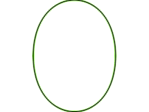
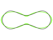
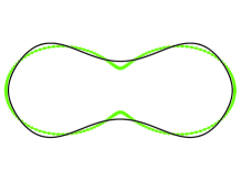
Figure 1: Profile of various test surfaces (black) and their reconstructions using surface harmonics with $N=4$ (green). The full surfaces are generated by rotation about thet $y$-axis. Left: prolate from [24], middle and right: red blood cell from [11] with 50% and 90% weight on tonicity 217 mO coefficients, respectively.

The surface harmonic parameterizations of these three surfaces are determined by

$$a_{n}^{m}=\displaystyle\int_{0}^{2\pi}\int_{0}^{\pi}r(\theta,\phi)S_{n}^{m}(\theta,\phi)\;d\theta\,d\phi.$$ (61)

For the reconstruction, the integration was computed numerically over 230 cubature points. Using the coefficients from (61), the reconstructed radius $\tilde{r}$ was determined by (18). The root mean square distance error in the reconstruction is defined over the cubature points by

$$E_{rmsd}=\displaystyle\sum_{i=1}^{230}(r(\theta_{i},\phi_{i})-\tilde{r}(\theta_{i},\phi_{i}))^{2}/230$$

The pointwise error and the relative error in the volume, surface area, and energy are provided in Tables 2-4 for various $N$.

$N$	$E_{rms}$	$E_{Vol}$	$E_{SA}$	$E_{Eng}$
1	$2.06\times 10^{-1}$	$2.57\times 10^{-2}$	$2.22\times 10^{-2}$	$3.73\times 10^{-2}$
2	$8.59\times 10^{-4}$	$2.22\times 10^{-4}$	$1.08\times 10^{-2}$	$8.37\times 10^{-3}$
3	$8.59\times 10^{-4}$	$2.22\times 10^{-4}$	$1.08\times 10^{-2}$	$8.37\times 10^{-3}$
4	$5.02\times 10^{-7}$	$2.56\times 10^{-6}$	$1.11\times 10^{-2}$	$7.19\times 10^{-3}$
5	$5.06\times 10^{-7}$	$2.56\times 10^{-6}$	$1.11\times 10^{-2}$	$7.19\times 10^{-3}$
6	$1.46\times 10^{-7}$	$2.76\times 10^{-6}$	$1.11\times 10^{-2}$	$7.18\times 10^{-3}$
7	$1.53\times 10^{-7}$	$2.76\times 10^{-6}$	$1.11\times 10^{-2}$	$7.18\times 10^{-3}$
8	$3.35\times 10^{-8}$	$2.76\times 10^{-6}$	$1.11\times 10^{-2}$	$7.18\times 10^{-3}$

Table 2: Error from truncation in surface harmonic expansion for prolate sample surface.

For the prolate surface, the reconstruction accuracy increases in all categories as $N$ increases. The most relevant observation to this work is that the error in the energy is less than 1% using $N=2$ and greater. For a simple prolate structure, only 9 modes are required.

$N$	$E_{rms}$	$E_{Vol}$	$E_{SA}$	$E_{Eng}$
1	$9.80\times 10^{-2}$	$4.00\times 10^{-1}$	$4.20\times 10^{-1}$	$4.21\times 10^{-1}$
2	$6.65\times 10^{-3}$	$4.80\times 10^{-2}$	$4.99\times 10^{-2}$	$8.36\times 10^{-1}$
3	$6.65\times 10^{-3}$	$4.80\times 10^{-2}$	$4.99\times 10^{-2}$	$8.36\times 10^{-1}$
4	$2.29\times 10^{-3}$	$1.93\times 10^{-3}$	$1.72\times 10^{-2}$	$5.34\times 10^{-2}$
5	$2.29\times 10^{-3}$	$1.93\times 10^{-3}$	$1.72\times 10^{-2}$	$5.34\times 10^{-2}$
6	$1.39\times 10^{-3}$	$4.94\times 10^{-3}$	$8.35\times 10^{-3}$	$1.62$
7	$1.39\times 10^{-3}$	$4.94\times 10^{-3}$	$8.35\times 10^{-3}$	$1.62$
8	$4.13\times 10^{-4}$	$3.29\times 10^{-5}$	$1.44\times 10^{-2}$	$7.97\times 10^{-1}$

Table 3: Error from truncation in surface harmonic expansion for RBC 1 (50% weight) sample surface.

$N$	$E_{rms}$	$E_{Vol}$	$E_{SA}$	$E_{Eng}$
1	$7.13\times 10^{-2}$	$2.82\times 10^{-1}$	$3.12\times 10^{-1}$	$3.82\times 10^{-1}$
2	$2.06\times 10^{-3}$	$1.35\times 10^{-2}$	$9.60\times 10^{-3}$	$3.96\times 10^{-1}$
3	$2.06\times 10^{-3}$	$1.35\times 10^{-2}$	$9.60\times 10^{-3}$	$3.96\times 10^{-1}$
4	$1.26\times 10^{-3}$	$3.36\times 10^{-3}$	$5.71\times 10^{-3}$	$7.75\times 10^{-2}$
5	$1.26\times 10^{-3}$	$3.36\times 10^{-3}$	$5.71\times 10^{-3}$	$7.75\times 10^{-2}$
6	$3.07\times 10^{-4}$	$1.92\times 10^{-3}$	$5.79\times 10^{-3}$	$4.24\times 10^{-1}$
7	$3.07\times 10^{-4}$	$1.92\times 10^{-3}$	$5.79\times 10^{-3}$	$4.24\times 10^{-1}$
8	$2.15\times 10^{-4}$	$1.21\times 10^{-3}$	$7.14\times 10^{-3}$	$9.97\times 10^{-2}$

Table 4: Error from truncation in surface harmonic expansion for RBC 2 (90% weight) sample surface.

For the red blood cell structures, initially the errors decrease as $N$ increases, but increasing the number of modes beyond a certain threshold actually increases the error in the energy computation. For RBC 1, the best possible error in the energy is 5.3%, with $N=4$ or $N=5$ modes. For RBC 2, the best error is 7.75% with the same $N$. We suggest the reason for this is because higher modes contain more bulges than the lower modes, akin to Runge’s phenomenon in high order polynomials. In the reconstruction, the coefficients are chosen to minimize $E_{rms}$. While transiently increasing $N$ does improve the accuracy of $E_{rms}$, it may introduce local oscillations. Since the energy is a function of the square mean curvature, these oscillations have a high energy cost. In Figure 2, RBC 1 is reconstructed with $N=4$ and $N=12$, for comparison.

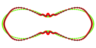
Figure 2: Effect of large $N$ for RBC 1. The analytical surface is in black, the reconstructed surfaces for $N=4$ and $N=12$ are in green and red, respectively. Increasing $N$ near 4 improves the pointwise accuracy especially near the edges, but also introduces oscillations near the center with high energy cost. For $N=12$, the pointwise error in the surface is improved at $1.18\times 10^{-4}$, but the error in the energy is 258%.

4 Examples: reduced volume

In this section, we provide numerical examples to test the robustness method. First, observe that the integration of the square local mean curvature $H^{2}$ is a dimensionless quantity. When the spontaneous curvature $C_{0}=0$, the mechanical bending energy (1) is completely governed by this dimensionless quantity and is therefore scale-invariant. Thus, for vesicle shapes, where $C_{0}=0$, the minimum energy is completely determined by a single dimensionless quantity called the reduced volume $v$. If we denote the current vesicle volume and surface area $V$ and $S_{A}$, respectively, then the reduced volume scales the current volume $V$ by the volume of a sphere with surface area $S_{A}$. Since spheres maximize volume for a given surface area, the reduced volume satisfies $v\leq 1$. The reduced volume is given by the formula

$$v=\displaystyle\frac{V}{4\pi/3R_{0}^{3}}$$ (62)

where $R_{0}=\sqrt{S_{A}/4\pi}$. In terms of the surface area, the reduced volume is

$$v=\displaystyle\frac{6\sqrt{\pi}V}{(S_{A})^{3/2}}.$$ (63)

Seifert et. al. has compiled a library of reduced volumes and their corresponding minimum energies for axisymmetric shapes in [24] by solving the Euler-Lagrange equations using a parameterization of the vesicle shape with an axis of symmetry. For verification purposes, we compare our axisymmetric results for various reduced volumes to theirs. We set the constraint volume $\bar{V}$ to be proportional to $V$ by the (projected) reduced volume $v$. The volume constraint is in violation and NCG begins to change the shape to relax this configuration. If we begin with a perfectly spherical vesicle, NCG will simply scale the sphere to a sphere with a smaller volume, and the final reduced volume will be 1. Therefore, we take a slightly perturbed sphere to be our initial configuration. After NCG has converged, we calculate the final reduced volume $v$ and the final energy $E$ scaled by the energy of a spherical vesicle $E_{0}=8\pi\mathscr{K}_{C}$.

From the reconstruction examples, $N=4$ is a reasonable truncation for the surface harmonic expansion. During the iterations of NCG, 20 cubature points are used. We say that NCG has converged when the norm of the change in gradient or if the change in the modes was less than $10^{-6}$. When the final configuration is achieved, the total energy is evaluated with 64 cubature points to provide a more accurate computation and to ensure that enough cubature points are used. For reduced volumes above approximately $v=0.75$, the numerical energy is within 10% of the analytical values calculated by Seifert et. al. (see Table 5. However, for reduced volumes less than this, the error exceeds 10%. If the number of modes is increased to $N=6$ (since $N=5$ gives the same numerical results as $N=4$ as demonstrated in Tables 2-4), the relative error is reduced. However, there is a significant difference between the energy evaluated at 20 cubature points than at 64 cubature points at the final iteration. This is because the added oscillation from the higher order modes is not absorbed by NCG with only 20 cubature points. Using 30 cubature points when $N=6$, the relative error is less than 1% when compared to 64 points. For surfaces with reduced volume $0.65\leq v\leq 0.75$, using $N=6$ and 30 cubature points, the relative error in the final energy is less than 10%. For surfaces with reduced volume $0.5\leq v<0.65$, we determined that 40 quadrature points are needed to use $N=8$; however, the error is still above 10%, and the use of $N=8$ fared no better than $N=6$. Our method could not reconstruct surfaces with these reduced volumes well. These data are plotted in Figure 3, overlayed by the analytic solution from Seifert [24].

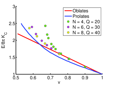
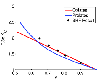
Figure 3: Vesicle energy vs. reduced volume for comparison with [24]. Left: All data points used to determine cutoff values for $N$ given a reduced volume $v$. Right: Kept data according to the cutoff values. All data points are within 10% error of the appropriate analytical curve.

In summary, for surfaces with $0.75\leq v\leq 1$, we used $N=4$ and 20 cubature points, for surfaces with $0.65\leq v<0.75$, we used $N=6$ and 30 cubature points. The results using this cutoff are overlayed by Seifert’s data in Figure 3. Finally, the surfaces corresponding to the data in Table 5 are shown in Figure 4.

$v$	1.0	0.90	0.81	0.76	0.70	0.65
$E/E_{0}$, [24]	1.0	1.19	1.37	1.58	1.72	1.85
$E/E_{0}$, SHF	1.0	1.22	1.45	1.61	1.76	1.99
Rel. error	0%	2.5%	5.8%	1.9%	2.3%	7.6%

Table 5: Vesicle energy vs. reduced volume for comparison with [13].

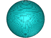
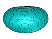
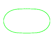
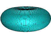
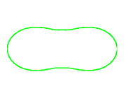
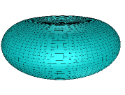
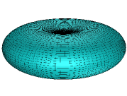
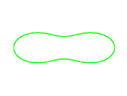
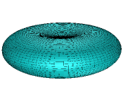
Figure 4: Axisymmetric results with various reduced volumes. Organized by row, $v=1.00,0.90;0.81,0.76;0.70,0.65$. The shapes here correspond to the data in Table 5. The full volumes are angled slightly down, while the profiles are not angled.

We note that the results of the numerical procedure may be only local minima and therefore only locally stable. With enough perturbation through some external force, another configuration with a lower energy may be achieved. In the range of $0.64\leq v\leq 1$, oblate shapes are local energy minimizers, but prolates are global minimizers for axisymmetric shapes. However, it may be possible to obtain a non-axisymmetric shape with lower energy than a prolate.

5 Conclusion

We have presented a fast algorithm for computing axisymmetric and non-axisymmetric spherical vesicles that correspond to minimized Canham-Helfrich-Evans curvature energy subject to surface area and volume constraints. Our method is based on the real-valued surface harmonic rather than the complex-valued spherical harmonic expansion of the surface configurations. Computational simulations showed that vesicles of various reduced volumes can be approximated using up to 49 surface harmonic functions, and the approximation error measured in curvature energy can be well maintained within 8%, mostly below 5% indeed. We use a nonlinear conjugate gradient method rather than the Newton’s method for the numerical minimization. This makes it possible for us to avoid the computation of the Hessian matrices and the solution of linear systems to further improve the efficiency of the calculation. Our method entails advantageous over the spherical harmonic approximations of the individual coordinates of the vesicle configurations since it excludes the complex parts unnecessary for computing real-valued surfaces [17]. We will explore the implementation of this fast algorithm in the external force fields such as fluid flow or electrostatic potential field, for which re-orientation of the vesicle configurations might be necessary because of the vesicle rotation caused by the non-vanishing torque applied by the external force. A fast algorithm for the vesicle deformation induced by the electrostatic force is currently under development and will be reported elsewhere.

Appendix A Nonlinear Conjugate Gradient Method and Linear Search

The pseudocode of the nonlinear conjugate method and the related linear search method is given below to ease the implementation. The functions $I(\cdot)$ and $\delta_{\Gamma}I(\cdot)$ evaluate the curvature energy and its gradient, c.f. Eqs. (3) and (4), respectively.

Algorithm 3.1: Nonlinear Conjugate Gradient
Given initial SHF modes $\vec{a}_{0}$, tolerances $\epsilon_{g},\epsilon_{a}$, $M$
Compute $E_{0}\leftarrow I(\vec{a}_{0})$, $\vec{g}_{0}\leftarrow\delta_{\Gamma}I(\vec{a}_{0})$
Direction $\vec{d}_{0}=-\vec{g}_{0}$
$k\leftarrow 0$
for $k=1:M$
  Step size $\alpha_{k}\leftarrow$ LineSearch$(\vec{a}_{k},\vec{d}_{k})$
  Step in direction $\vec{a}_{k+1}\leftarrow\vec{a}_{k}+\alpha_{k}\vec{d}_{k}$
  Update energy and gradient $E_{k+1}\leftarrow I(\vec{a}_{k+1})$, $\vec{g}_{k+1}\leftarrow\delta_{\Gamma}I(\vec{a}_{k+1})$
  if $||\vec{g}_{k+1}-\vec{g}_{k}||<\epsilon_{g}$   break
  Compute $\beta_{k}\leftarrow(\vec{g}_{k+1}^{T}(\vec{g}_{k+1}-\vec{g}_{k}))/((\vec{g}_{k+1}-\vec{g}_{k})^{T}\vec{d}_{k})$
  Update direction $\vec{d}_{k+1}\leftarrow-\vec{g}_{k+1}+\beta_{k}\vec{d}_{k}$
  if $||\vec{a}_{k+1}-\vec{a}_{k}||<\epsilon_{a}$   break
  $k\leftarrow k+1$
end
return $\vec{a}_{k}$

Algorithm 3.2: LineSearch$(\vec{a},\vec{d})$
Define $\alpha_{m}\leftarrow 0,\alpha_{M}\leftarrow 1,M,\epsilon$
Compute $E_{m}\leftarrow I(\vec{a}+\alpha_{m}\cdot\vec{d})$, $E_{M}\leftarrow I(\vec{a}+\alpha_{M}\cdot\vec{d})$
if $E_{m}<E_{M}$
  $\alpha_{l}\leftarrow\alpha_{m}$; $\alpha_{u}\leftarrow\alpha_{M}$
  $E_{l}\leftarrow E_{m}$; $E_{u}\leftarrow E_{M}$
else
  $\alpha_{l}\leftarrow\alpha_{M}$; $\alpha_{u}\leftarrow\alpha_{m}$
  $E_{l}\leftarrow E_{M}$; $E_{u}\leftarrow E_{m}$
end if
for $i=1:M$
  $\alpha_{t}\leftarrow(\alpha_{l}+\alpha_{u})/2$
  $E_{t}\leftarrow I(\vec{a}+\alpha_{t}\cdot\vec{d})$
  if $E_{t}>E_{l}$ then
    $\alpha_{u}\leftarrow\alpha_{t}$
  else
    $\vec{g}\leftarrow\delta_{\Gamma}I(\vec{a}+\alpha_{t}\cdot\vec{d})$
    $(D\phi)\leftarrow\vec{g}^{T}\,\vec{d}$
    if $(D\phi)\cdot(\alpha_{l}-\alpha_{t})>0$ then
      $\alpha_{l}\leftarrow\alpha_{t}$
    else
      $\alpha_{u}\leftarrow\alpha_{l}$; $\alpha_{l}\leftarrow\alpha_{t}$
    end if
    $E_{l}\leftarrow E_{t}$
  end if
  if $|\alpha_{u}-\alpha_{l}|<\epsilon$   break
return $\alpha_{t}$

References

- [1] Prosenjit Bagchi. Mesoscale simulation of blood flow in small vessels. Biophys. J., 92(6):1858 – 1877, 2007.
- [2] Amir Houshang Bahrami and Mir Abbas Jalali. Vesicle deformations by clusters of transmembrane proteins. J. Chem. Phys., 134:085106, 2011.
- [3] P.B. Canham. The minimum energy of bending as a possible explanation of the biconcave shape of the human red blood cell. J. Theor. Biol., 26(1):61 – 81, 1970.
- [4] R. Capovilla, J. Guven, and J. A. Santiago. Deformations of the geometry of lipid vesicles. J. Phys. A - Math. Gen., 36(23):6281, 2003.
- [5] Sovan Das and Qiang Du. Adhesion of vesicles to curved substrates. Phys. Rev. E, 77:011907, Jan 2008.
- [6] Qiang Du, Chun Liu, Rolf Ryham, and Xiaoqiang Wang. A phase field formulation of the willmore problem. Nonlinearity, 18:1249, 2005.
- [7] Qiang Du, Chun Liu, and Xiaoqiang Wang. A phase field approach in the numerical study of the elastic bending energy for vesicle membranes. J. Comput. Phys., 198(2):450 – 468, 2004.
- [8] Qiang Du, Chun Liu, and Xiaoqiang Wang. Simulating the deformation of vesicle membranes under elastic bending energy in three dimensions. J. Comput. Phys., 212(2):757 – 777, 2006.
- [9] C. D. Eggleton and A. S. Popel. Large deformation of red blood cell ghosts in a simple shear flow. Phys. Fluids, 10(8):1834–1845, 1998.
- [10] E.A. Evans. Bending resistance and chemically induced moments in membrane bilayers. Biophys. J., 14(12):923–931, 1974.
- [11] Evan Evans and Yuan-Cheng Fung. Improved measurements of the erythrocyte geometry. Microvasc. Res., 4(4):335 – 347, 1972.
- [12] Khashayar Farsad and Pietro De Camilli. Mechanisms of membrane deformation. Curr. Opin. Cell Biol., 15(4):372 – 381, 2003.
- [13] Feng Feng and William S. Klug. Finite element modeling of lipid bilayer membranes. J. Comput. Phys., 220(1):394 – 408, 2006.
- [14] Volkmar Heinrich, Bojan Bozic, Sasa Svetina, and Bostjan Zeks. Vesicle deformation by an axial load: From elongated shapes to tethered vesicles. Biophys. J., 76:2056–2071, 1999.
- [15] W. Helfrich et al. Elastic properties of lipid bilayers: theory and possible experiments. Z. Naturforsch. C, 28(11):693–703, 1973.
- [16] Roger D. Kamm. cellular fluid mechanics. Annu. Rev. Fluid Mech., 34(1):211–232, 2002.
- [17] Khaled Khairy and Jonathon Howard. Minimum-energy vesicle and cell shapes calculated using spherical harmonics parameterization. Soft Matter, 7:2138–2143, 2011.
- [18] Shuwang Li, John Lowengrub, and Axel Voigt. Locomotion, wrinkling, and budding of a multicomponent vesicle in viscous fluids. Commun. Math. Sci., 10:645–670, 2012.
- [19] L. Ma and W. S. Klug. Viscous regularization and r-adaptive remeshing for finite element analysis of lipid membrane mechanics. J. Comput. Phys., 227(11):5816–5835, 2008.
- [20] M. Mikucki and Y. Zhou. Electrostatic forces on charged surfaces of bilayer lipid membranes. SIAM J. Appl. Math., 74(1):1–21, 2014.
- [21] Jorge Nocedal and Stephen J. Wright. Numerical optimization. Springer series in operations research and financial engineering. Springer, New York, NY, 2. ed. edition, 2006.
- [22] Thomas R. Powers. Mechanics of lipid bilayer membranes. In Sidney Yip, editor, Handbook of Materials Modeling, pages 2631–2643. Springer Netherlands, 2005.
- [23] Udo Seifert. Configurations of fluid membranes and vesicles. Adv. Phys., 46(1):13–137, 1997.
- [24] Udo Seifert, Karin Berndl, and Reinhard Lipowsky. Shape transformations of vesicles: Phase diagram for spontaneous- curvature and bilayer-coupling models. Phys. Rev. A, 44:1182–1202, Jul 1991.
- [25] Jin Sun Sohn, Yu-Hau Tseng, Shuwang Li, Axel Voigt, and John S. Lowengrub. Dynamics of multicomponent vesicles in a viscous fluid. J. Comput. Phys., 229(1):119 – 144, 2010.
- [26] I.S. Sokolnikoff. Tensor analysis: theory and applications to geometry and mechanics of continua. Applied mathematics series. Wiley, 1964.
- [27] Jerome Solon, Olivier Gareil, Patricia Bassereau, and Yves Gaudin. Membrane deformations induced by the matrix protein of vesicular stomatitis virus in a minimal system. J. Gen. Virol., 86(12):3357–3363, 2005.
- [28] Knut Erik Teigen, Peng Song, John Lowengrub, and Axel Voigt. A diffuse-interface method for two-phase flows with soluble surfactants. J. Comput. Phys., 230:375 – 393, 2011.
- [29] Xiaoqiang Wang and Qiang Du. Modelling and simulations of multi-component lipid membranes and open membranes via diffuse interface approaches. J. Math. Biol., 56:347–371, 2008.
- [30] Guo-Wei Wei. Differential geometry based multiscale models. Bulletin of Mathematical Biology, 72(6):1562–1622, 2010.
- [31] Steven Wise, Junseok Kim, and John Lowengrub. Solving the regularized, strongly anisotropic cahn–hilliard equation by an adaptive nonlinear multigrid method. J. Comput. Phys., 226(1):414 – 446, 2007.
- [32] Jian-Jun Xu, Yin Yang, and John Lowengrub. A level-set continuum method for two-phase flows with insoluble surfactant. J. Comput. Phys., 231(17):5897 – 5909, 2012.
- [33] Xiaofeng Yang, Ashley J. James, John Lowengrub, Xiaoming Zheng, and Vittorio Cristini. An adaptive coupled level-set/volume-of-fluid interface capturing method for unstructured triangular grids. J. Comput. Phys., 217(2):364–394, 2006.
- [34] Ou-Yang Zhong-can and W. Helfrich. Instability and deformation of a spherical vesicle by pressure. Phys. Rev. Lett., 59:2486–2488, 1987.
- [35] Y. C. Zhou, B. Lu, and A. A. Gorfe. Continuum electromechanical modeling of protein-membrane interactions. Phys. Rev. E, 82(4):041923, 2010.