Edge-state enhanced transport in a 2-dimensional quantum walk

Abstract

Quantum walks on translation invariant regular graphs spread quadratically faster than their classical counterparts. The same coherence that gives them this quantum speedup inhibits, or even stops their spread in the presence of disorder. We ask how to create an efficient transport channel from a fixed source site (A) to fixed target site (B) in a disordered 2-dimensional discrete-time quantum walk by cutting some of the links. We show that the somewhat counterintuitive strategy of cutting links along a single line connecting A to B creates such a channel. The efficient transport along the cut is due to topologically protected chiral edge states, which exist even though the bulk Chern number in this system vanishes. We give a realization of the walk as a periodically driven lattice Hamiltonian, and identify the bulk topological invariant responsible for the edge states as the quasienergy winding of this Hamiltonian.

I Introduction

The Discrete-Time Quantum Walk (DTQW, or quantum walk for short)Kempe (2003), a quantum mechanical generalization of the random walk, has in the recent years received more and more attention from both the theoretical and experimental side. The main drive to understand the properties of the DTQW come from its possible use for quantum information processing, be it quantum search algorithmsShenvi et al. (2003), or even general purpose quantum computationLovett et al. (2010). Experiments on quantum walks range from realizations on trapped ionsTravaglione and Milburn (2002); Zähringer et al. (2010); Schmitz et al. (2009), to cold atoms in optical latticesKarski et al. (2009); Genske et al. (2013), and on light on an optical tableSchreiber et al. (2010, 2012); Peruzzo et al. (2010); Broome et al. (2010); Sansoni et al. (2012), but there are many other experimental proposalsCôté et al. (2006); Kálmán et al. (2009).

The distinguishing feature of quantum walks is that on regular graphs, they spread faster than their classical counterparts: the root-mean-square distance of the walker from the origin increases with the number $N$ of steps as $\mathcal{O}(N)$, rather than $\mathcal{O}(\sqrt{N})$ as in the classical case. This can be put to good use for algorithms based on quantum walksShenvi et al. (2003) that find a marked state among $N$ states in only $\mathcal{O}(\sqrt{N})$ steps, outperforming their classical counterparts – the same scaling advantage as of the Grover algorithmGrover (1997), which can also be understood as a DTQW. The intuitive explanation for this ballistic scaling is that a DTQW can be seen as a stroboscopic simulator for an effective Hamiltonian, and thus, in a clean system, its eigenstates are plane waves.

If we understand a DTQW to be a stroboscopic simulator for a Hamiltonian, we can expect that static disorder can impede the spreading of the walk, even bringing it to a complete standstill, through Anderson localizationLagendijk et al. (2009). This prediction has been mathematically proven for some types of one-dimensional DTQWsJoye and Merkli (2010); Ahlbrecht et al. (2011), and even observed in an optical implementation Schreiber et al. (2011). However, even in one dimension, some types of disorder lead to a slow, subdiffusive spreading of the walk rather than complete localizationObuse and Kawakami (2011); this phenomenon can also be explained in terms of the effective HamiltonianObuse and Kawakami (2011); Brouwer et al. (2000). Two-dimensional DTQWs are also expected to suffer Anderson localizationSvozilík et al. (2012), although in some cases disorder causes diffusionEdge and Asboth (2014).

In this paper we address the question: is there a way to create an efficient transport channel in a 2-dimensional split-step DTQW (2DQW) that defeats localization even if static disorder is present? We take a DTQW on a square lattice, with two special sites: $A$, where the walk is started from, and $B$, where we want the walker to ultimately end up, rather than escaping to infinity or remaining in the vicinity of $A$. To create a channel, we cut links on the lattice, thus restricting the movement of the walker. The first idea, cutting out a narrow island, with $A$ on the one end, and $B$ on the other, is rendered ineffective by static disorder. We find a somewhat counterintuitive strategy that does work, however: cutting the links along a single line connecting $A$ to $B$ creates a conveyor belt for the walker, transporting it efficiently and ballistically from $A$ to $B$ even in the presence of considerable amount of static disorder.

The way that a cut along a line on the lattice of the quantum walk forms a robust conveyor belt for the walker is reminiscent of how electrons are transported along line defects by edge states in topological insulatorsHasan and Kane (2010). This seems to be a promising direction for an understanding of the transport mechanism, since the effective Hamiltonians of DTQWs can be engineered to realize all classes of topological phases in 1 and 2 dimensionsKitagawa et al. (2010). However, the effective Hamiltonian of the 2DQW is topologically trivialKitagawa et al. (2010). Thus, if there is a bulk topological invariant protecting these states from disorder, it is not covered by standard theoryRyu et al. (2010).

The topological structure of DTQWs is in fact richer than that of time-independent Hamiltonians, and exploration of that structure is far from complete. The telltale signs of extra topology are protected edge states at the edges of bulks where the topological invariants of the effective Hamiltonian predict none. An example is one-dimensional DTQWs with chiral symmetry, where such edge states have been detected in an optical experimentKitagawa et al. (2012), and have been predicted to exist between two bulks with the same effective HamiltonianAsbóth (2012). In that case, the extra topological structure responsible for the protection of these states has been found, and can be described based on time-delayed effective HamiltoniansAsbóth and Obuse (2013), scattering matricesTarasinski et al. (2014), or as winding numbers of one part of the timestep operatorAsbóth et al. (2014a). Edge states between two bulks in the 2DQW have been found numericallyKitagawa (2012), but the extra topological invariants that they indicate are unknown.

In this paper we show that there are chiral (one-way propagating) edge states along a cut in a 2DQW, and identify the bulk topological invariant responsible for their appearance. We map the quantum walk to a periodically driven Hamiltonian, and thus identify the invariant as the winding number found by Rudner et al.Rudner et al. (2013), which we refer to as Rudner invariant.

The paper is structured as follows. We introduce the type of 2DQW we consider, together with the prescription of how to cut links on the graph, in Section II. Then, in Section III, we consider two strategies to enhance transport in the 2DQW: in a clean case, the straightforward, “island cut” approach works fine, but in the presence of disorder, only the less intuitive, “line cut” approach gives efficient transport. We show that there are edge states along the line cut in Section IV. In Section V we find the bulk topological invariants responsible for the edge states. In Sect. VI we consider the effects of disorder on the edge state transport.

II Definitions

Of the wide variety of two-dimensional quantum walks, we choose the split-step walk on a square lattice (2DQW), defined in Ref. Kitagawa et al., 2010, for its simplicity: it requires only two internal states for the walker. In this section we recall the definition of the 2DQW, introduce the conditional wavefunction method which allows us to treat transport in the quantum walk setting, discuss how to cut links in the quantum walk and how disorder is introduced.

Figure 1: Layout of the 2-dimensional quantum walk, with a source at $A$, a detector at the target site at $B$, and detectors at the edges. For the conditional wavefunction, the detectors play the role of absorbers.

II.1 Walker wavefunction and time evolution operator

We consider a particle, or walker, on a square lattice, with two internal states, which we refer to as spin. The wavefunction of the walker can be written as

$$|{\Psi}\rangle =\sum_{\vec{r}\in\mathcal{D}}(\Psi(\vec{r},\uparrow)|{\vec{r},\uparrow}\rangle+\Psi(\vec{r},\downarrow)|{\vec{r},\downarrow}\rangle).$$ (1)

Here $\vec{r}=(x,y)$ is a 2-dimensional vector of integers, which labels the nodes of the lattice, taken from $\mathcal{D}=\{(x,y)|x=1,\ldots,x_{\text{max}},y=1,\ldots,y_{\text{max}}\}$. The walker is initialized at site $A=(x_{A},y_{A})$ as

$$|{\Psi(t=0)}\rangle =|{A,\uparrow}\rangle.$$ (2)

The dynamics of the walker takes place in discrete time $t\in\mathbb{N}$, and is determined by

$$|{\Psi(t+1)}\rangle =U|{\Psi(t)}\rangle;$$ (3)

$$U =S_{y}R_{2}S_{x}R_{1}.$$ (4)

The operator $R_{j}$, with $j=1,2$, denotes a rotation of the spin about the $y$ axis,

$$R_{j} =\sum_{\vec{r}\in\mathcal{D}}|{\vec{r}}\rangle\langle{\vec{r}}|\otimes e^{-i\theta_{j}(\vec{r})\sigma_{y}}.$$ (5)

The angles $\theta_{1}$ and $\theta_{2}$ of the first and second rotation can depend on the position $\vec{r}=(x,y)$ of the walker. The operators $S_{x}$ and $S_{y}$ denote spin-dependent translations along links between the sites on the lattice,

$$S_{x} =\sum_{\vec{r}\in\mathcal{D}}|{\vec{r}+\hat{x},\uparrow}\rangle\langle{\vec{r},\uparrow}|+|{\vec{r},\downarrow}\rangle\langle{\vec{r}+\hat{x},\downarrow}|;$$ (6)

$$S_{y} =\sum_{\vec{r}\in\mathcal{D}}|{\vec{r}+\hat{y},\uparrow}\rangle\langle{\vec{r},\uparrow}|+|{\vec{r},\downarrow}\rangle\langle{\vec{r}+\hat{y},\downarrow}|,$$ (7)

where $\hat{x}=(1,0)$ and $\hat{y}=(0,1)$.

II.2 Conditional wavefunction

We want to measure how efficient transport is to a given site, $B=(x_{B},y_{B})$, as opposed to propagation to the boundary of the system, denoted by the sites $C_{j}$, as shown in Fig. 1. We place a detector at site $B$, and at the boundary sites $C_{j}$. After every timestep, each detector performs a dichotomic measurement on the wavefunction: if the walker is at the detector, it is detected, if not, it is undisturbed. To calculate the resulting probability distribution for the transmission times, we compute the conditional wavefunction $|{\Psi(t)}\rangle$, conditioned on no detection events up to time $t$. To obtain the time evolution of the conditional wavefunction, at the end of each timestep the components of the wavefuntion at the sites $B$ and $C_{j}$ are projected out,

$$\Psi(t) =\Big{(}1-|{B}\rangle\langle{B}|-\sum_{j}|{C_{j}}\rangle\langle{C_{j}}|\Big{)}U|{\Psi(t-1)}\rangle.$$ (8)

Note that measurements are performed at each step, but since the measurement record is kept, the whole process is still completely coherent.

The norm of the walker’s wavefunction, $\langle{\Psi(t)}|{\Psi(t)}\rangle$, is the probability that the particle is still in the system after $t$ steps. Due to the postselection involved in the timestep, Eq. (8), this norm decreases over time as the walker is found at $B$ (successful transmission) or leaks out at the edges (transmission failure). The probability of success, i.e., of detecting the walker at $B$ at time $t$, is given by

$$p_{t} =\sum_{s=\uparrow,\downarrow}\left|{\langle{B,s}|U|{\Psi(t-1)}\rangle}\right|^{2}.$$ (9)

The arrival probability at time $t$ is the summed probabilities of absorption up to time $t$ and is given by

$$P_{t}=\sum_{t^{\prime}=1}^{t}p_{t^{\prime}}$$ (10)

II.3 Disorder through the rotation angles.

We will consider the effects of disorder that enters the system through the angles $\theta$. The rotation angles become position dependent, uncorrelated random variables, chosen from a uniform distribution,

$$\theta_{j}(\vec{r})\in[\theta_{j}-\delta,\theta_{j}+\delta].$$ (11)

In this paper we will consider time-independent (i.e., static, or quenched) disorder, i.e., the angles $\theta$ depend only on position, but not on time. The effects of disorder will be addressed in section VI.

II.4 Cutting links

To enhance transport, we consider modifying the graph on which the walk takes place by cutting some of the links. If the link between sites $(x,y)$ and $(x+1,y)$ is cut, the $\uparrow$ component of the wavefunction is not transported from site $(x,y)$ to $(x+1,y)$ during the $S_{x}$ shift operation and similarly the $\downarrow$ component from $(x+1,y)$ is not shifted to $(x,y)$. The analogous definition for cut links holds for the $S_{y}$ operation between sites $(x,y)$ and $(x,y+1)$.

If we were dealing with a lattice Hamiltonian instead of a lattice timestep operator, cutting a link could be done by just setting the corresponding hopping amplitude to 0. In the case of the timestep operator, however, maintaining the unitary of the time evolution – orthogonal states always have to stay orthogonalAsbóth (2012) – is more involved. The only sensible unitary and short-range way to do that is to induce a spin flip instead of a hop, with possibly an additional phase factor. This extra phase plays an important role in the 1D quantum walk, where it affects the quasienergy of the end statesAsbóth (2012). For 2D quantum walks, however, this extra phase factor unimportant. For convenience, we flip the spin using $-i\sigma_{y}$.

The complete shift operator $S_{d}$, with $d=x$ or $y$, including the prescription for cutting the links, reads

$$S_{d} =\sum_{\vec{r}\in\mathcal{L}_{d}}\left(|{\vec{r}+\hat{d},\uparrow}\rangle\langle{\vec{r},\uparrow}|+|{\vec{r},\downarrow}\rangle\langle{\vec{r}+\hat{d},\downarrow}|\right)$$

$$\quad+\sum_{\vec{r}\in\mathcal{C}_{d}}\left(|{\vec{r},\downarrow}\rangle\langle{\vec{r},\uparrow}|-|{\vec{r}+\hat{d},\uparrow}\rangle\langle{\vec{r}+\hat{d},\downarrow}|\right).$$ (12)

Here $\mathcal{L}_{d}$ is the set of vectors $\vec{r}$ such that the link between node at $\vec{r}$ and the node at $\vec{r}+\hat{d}$ is not cut, while its complement $\mathcal{C}_{d}$ is the set of vectors to nodes $\vec{r}$ for which the link connecting them to node $\vec{r}+\hat{d}$ has been cut, with $\hat{d}$ denoting the unit vector in the direction $d$ (i.e., $\hat{x}$ or $\hat{y}$).

III Transport in the presence of a cut

We now address the question: which links should we cut to optimize the transport from A to B? The first idea that comes to mind to ensure efficient transport is to cut out a narrow island from the lattice: at the one end of the island is $A$, the source, at the other end $B$, the site where we want the walker to be transported to. However, as we see, in the presence of disorder, there is a much more efficient construction.

III.1 The island cut

Figure 2: To increase the efficiency of transport from $A$ to $B$, the first idea is to cut an island that will form a transport channel, as indicated by the dashed line. All links crossing the dashed line are cut; a particle attempting to hop across a cut link will have its spin flipped instead of hopping.

Perhaps the most straightforward way to ensure that the walker gets from $A$ to $B$ is to restrict its motion to a narrow island connecting these two sites, by cutting links as illustrated in Fig. 2. In a clean system, this strategy achieves the desired effect. Simulations on large system sizes, shown in Fig. 3.a, show a high success probability, independent of system size (island length), with a time required for transport proportional to the length of the island, indicating ballistic transport.

The simple strategy of cutting out an island to guide the walker to $B$ no longer works if there is quenched disorder in the rotation angles. As shown in Fig. 3b), the time evolution of the walker’s wavefunction now shows signs of localization. With a disorder of $\delta\theta=0.07\pi$, the average distance from the origin stops growing after some time, independent of system size.

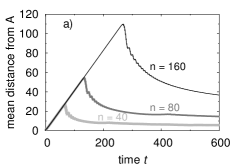
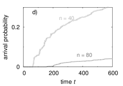
Figure 3: Mean displacement of the quantum walker (continuous lines) and transmission probability (dotted lines) in the geometry of the “island” of Fig. 2, for a horizontal island of fixed width of 1, and varying island length of 40 (thick light gray), 80 (medium gray), and 160 (thin black). Mean rotation angles are set to $\theta_{1}=0.35\pi$, $\theta_{2}=0.15\pi$. Without disorder, $\delta=0$, the wavefunction spreads ballistically (a) and the transmission probability reaches a value close to 1 as the wavepacket arrives (b). To illustrate the effects of disorder, we set $\delta=0.2\pi$, and use a single disorder realization, varying only the distance $n$ between $A$ and $B$ (and correspondingly, the length of the island). For large enough system ($n=160$), the mean distance from $A$ saturates at around 30 (c), and in this case there is virtually no transmission ((d): $P_{t}<10^{-4}$ for $n=160$ for all times $t$).

III.2 The single line cut

There is a somewhat counterintuitive strategy to defeat localization, and ensure efficient transport from $A$ to $B$ even with static disorder. This involves cutting links along a line from A to B, as shown in Fig. 4.

As shown in Fig. 5, in spite of the disorder, the single cut ensures ballistic propagation of the quantum walker and greatly enhances the transmission probability: the line of cut links acts like a conveyor belt for the quantum walker. Although for the detailed numerics we used cuts that are along a straight line, numerical examples convincingly show that the shape of the cut can delay the transport, but not inhibit it. For an example, see the Appendix A.

Figure 4: An alternative strategy to create a channel between $A$ and $B$ is a single cut.

Figure 5: Mean displacement of the quantum walker (a, continuous lines) and transmission probability (b, dotted lines) in the geometry of the “single cut” of Fig. 4, for a horizontal cut. A single realization of a disordered quantum walk is taken, with mean rotation angles $\theta_{1}=0.35\pi$, $\theta_{2}=0.15\pi$, and disorder $\delta=0.3\pi$. The $A-B$ distance $n$ is varied: $n=40$ (thick light gray), $n=80$ (medium gray), and $n=160$ (thin black). The walker propagates ballistically along the cut (b), and arrives at $B$ with a high probability (c).

The rest of this paper is devoted to this conveyor belt mechanism. Our principal aims will be to answer the following two questions: Why does the conveyor mechanism work? How robust is it?

IV Edge states along a cut

In this section we show that the single cut transports the walker efficiently from the source $A$ to the target site $B$ because the quantum walk has unidirectional (chiral) edge states along the cut. We find the edge states along the cut using the effective Hamiltonian.

The effective Hamiltonian $H_{\textrm{eff}}$ of a DTQW is defined as

$$H_{\textrm{eff}} =i\log U,$$ (13)

where $U$, as in Eq. (4), is the unitary timestep operator of the quantum walk without the projectors corresponding to the measurements. We fix the branch cut of the logarithm to be along the negative part of the real axis. If we only look at the DTQW at integer times $t$, we cannot distinguish a DTQW from the time evolution that would be produced by the time-independent lattice Hamiltonian $H_{\textrm{eff}}$, since,

$$|{\Psi(t)}\rangle =U^{t}|{\Psi(0)}\rangle=e^{-iH_{\textrm{eff}}t}|{\Psi(0)}\rangle\,\,\text{ for }t\in\mathbb{N}.$$ (14)

Every DTQW is thus a stroboscopic simulator for its effective Hamiltonian $H_{\textrm{eff}}$.

We now consider the quasienergy dispersion relation of a clean system in the vicinity of (below) a horizontal cut, as shown in Fig. 6. We make use of translation invariance, and use $k$ to denote the quasimomentum along $x$, a conserved quantity. We take system of width $1$ ($x=1$) and height $L$ ($y=1,\ldots,L$), with modified periodic boundary conditions along both directions. Along $x$, twisted boundary conditions are taken, i.e., periodic boundary conditions with an extra phase factor of $e^{\mp ik}$ for right/left shifts, with $k$ denoting the quasimomentum we are interested in. Along $y$, we leave the periodic boundary conditions, but cut the link connecting site $(1,L)$ with $(1,1)$, and we insert an absorber at $(1,1)$. We diagonalize the timestep operator $U$ on this system, obtaining the eigenvalues $\lambda_{n}=\left|{\lambda_{n}}\right|e^{-i\varepsilon_{n}}$ and the corresponding eigenvectors $|{\Psi}\rangle_{n}$. The magnitudes $\left|{\lambda_{n}}\right|\leq 1$ give us information about the lifetime of the states, while the phases $\varepsilon_{n}$ can be identified with the quasienergies. Repeating this procedure for $-\pi<k\leq\pi$ gives us the dispersion relation of a clean strip with a cut at the top and absorbers at the bottom.

We show the numerically obtained dispersion relation of the 2DQW on a stripe with an edge in Fig. 7. We omitted states with short lifetimes, whose eigenvalue of $U$ has magnitude $\left|{\lambda}\right|<0.9$. We used thick (blue) to highlight edge states, defined as states for which $\left|{\langle{L}|{\Psi}\rangle}\right|^{2}+\left|{\langle{L-1}|{\Psi}\rangle}\right|^{2}+\left|{\langle{L-2}|{\Psi}\rangle}\right|^{2}>0.9$. Whenever the gaps around $\varepsilon=0$ and $\varepsilon=\pi$ are open, one can clearly see edge states traversing these gaps. The edge states are unidirectional (i.e., chiral), and propagate in the same direction in the two gaps.

We obtained simple analytical formulas for the dispersion relations of the edge states along the horizontal cut, for $\varepsilon\approx 0$ and $\varepsilon\approx\pi$, using the transfer matrix method. We relegate the details to the Appendix B, and summarize the main results here. When $\sin(\theta_{1}+\theta_{2})>0$, the edge states are around $k=\varepsilon=0$ and $k=\varepsilon=\pm\pi$ (as in Fig. 7a-d), when $\sin(\theta_{1}+\theta_{2})<0$, they are around $k=\pm\pi,\varepsilon=0$ and $k=0,\varepsilon=\pm\pi$ (as in Fig. 7f). Near the center of the gaps, the edge states group velocity reads

$$v=\frac{d\varepsilon}{dk} =\sin(\theta_{2}-\theta_{1})\text{ sign }\left[\sin(\theta_{1}+\theta_{2})\right].$$ (15)

The edge states decay exponentially towards the bulk as $\Psi\propto e^{-\left|{y}\right|/\xi}$, where $y$ is the distance from the edge. Using the analytical calculations of Appendix B, we obtain the penetration depth $\xi$ of the edge states into the bulk as

$$\xi =-\left(\text{log }\frac{1-\left|{\sin(\theta_{1}+\theta_{2}}\right|}{\left|{\cos(\theta_{1}-\theta_{2})}\right|}\right)^{-1}.$$ (16)

Although the penetration depth and the magnitude of the group velocity can depend on the orientation of the edge, the direction of propagation of these chiral edge states constitutes a topological invariant. We show this topologically protected quantity as a function of the parameters $\theta_{1}$ and $\theta_{2}$ by boldface numbers in Fig. 8.

The direction of propagation (chirality) of the edge states is topologically protected: it can only be changed if the rotation angles $\theta_{j}$ are themselves changed so that the system is taken across a gap closing point. There are two different scenarios here, corresponding to gap closings where $\theta_{1}-\theta_{2}=n\pi$ (lines slanting upwards in Fig. 8, e.g., labels (a)-(c) in Figs. 7 and 8), and where $\theta_{1}+\theta_{2}=n\pi$ (lines slanting downwards in Fig. 8, e.g., labels (d)-(f) in Figs. 7 and 8). In the first case, during the gap closing, the number of edge states constituting the edge mode does not change, their penetration depth, Eq. (16) stays finite, it is only the edge mode velocity that goes to zero and then changes sign, see Eq. (15). In the second case, the velocity of the edge mode does not change as the gap is closed; it is the number of edge states that goes to zero and then grows again. In this case, the penetration depth $\xi$ diverges as the gap is closed. The two scenarios of this paragraph correspond to edge states at a zigzag or an armchair edge in the Haldane modelHaldane (1988) (e.g., Fig. 5. of Ref. Gómez-León et al., 2014).

Figure 6: For the analytical calculation, we consider a simple geometry with reflecting edge on top, and absorbers on the bottom. An infinite strip (left) can be treated as a 1-dimensional chain with twisted boundary conditions, i.e. with periodic boundaries along $x$ with an extra phase of $e^{\pm ikx}$ for right/left hopping. The top three rows, with dark (blue) background are defined as the edge region.

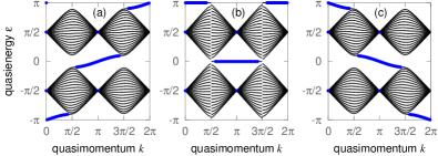
Figure 7: Dispersion relation of a 2DQW on a strip with cut links on top, and absorbers at the bottom. Quasienergies of long-lived states (magnitude of Floquet eigenvalue higher than $0.9$) are shown, with edge states (more than 80% of the weight on the top three rows) highlighted in thick (blue). The bulk gap is closed and reopened by setting the rotation angles to (a): $\theta_{1}=0.35\pi$, $\theta_{2}=0.15\pi$, (b): $\theta_{1}=\theta_{2}=0.25\pi$, (c): $\theta_{1}=0.15\pi$, $\theta_{2}=0.35\pi$. (d): $\theta_{1}=0.65\pi$, $\theta_{2}=0.15\pi$, (e): $\theta_{1}=0.75\pi$, $\theta_{2}=0.25\pi$, (f): $\theta_{1}=0.85\pi$, $\theta_{2}=0.35\pi$.

Figure 8: Parameter space of the split-step 2D discrete-time quantum walk. Along continuous (dotted) lines, the bulk quasienergy gap around 0 ($\pi$) quasienergy closes. Each gapped domain supports edge states near a cut, at both quasienergies 0 and $\pi$. The number of these edge states (equal to the Rudner winding number as per Eq. (22)), is written in bold. The Chern number, which is always 0 due to the sublattice symmetry, is shown in normal typeface.

V Topological invariant of the 2-dimensional split-step quantum walk

In a free lattice system with unitary dynamics, the number of unidirectional (chiral) edge states in the bulk energy gap cannot be altered by any local changes in the dynamics, as long as the bulk energy gap is open. Thus, the number of such edge states constitutes a topological invariant for each bulk gap. In time-independent lattice Hamiltonians, this invariant can be obtained from the bulk Hamiltonian as the sum of the Chern numbers of all the bands with energy below the gap. The Chern number for the bands of the 2DQW, however, is always zero, due to a discrete sublattice symmetry of the timestep operator, as we show in Appendix C. Thus, there has to be some other bulk topological invariant of the 2DQW. This extra topological invariant is also indicated by the fact that edge states appear at an interface between two domains of the 2DQW with the same Chern numberKitagawa (2012). We will now identify this bulk topological invariant.

V.1 The Rudner Invariant in periodically driven quantum systems

A candidate for the topological invariant of the 2DQW is the winding number of periodically driven 2-dimensional lattice Hamiltonians found by Rudner et al.Rudner et al. (2013), which we summarize here. Consider a periodically driven lattice Hamiltonian,

$$H(t+1,k_{x},k_{y}) =H(t,k_{x},k_{y}).$$ (17)

The unitary time evolution operator for one complete period reads

$$U(k_{x},k_{y}) =\mathbb{T}e^{-i\int_{0}^{1}H(k_{x},k_{y},t)dt}.$$ (18)

Next, define a loop in the following way,

$$U_{2}(t,k_{x},k_{y})=\left\{\begin{array}[]{rl}\mathbb{T}e^{-2i\int_{0}^{t}H(k_{x},k_{y},2t^{\prime})dt^{\prime}}&\mbox{ if $t<\frac{1}{2}$}\\ e^{2i(t-1/2)H_{\textrm{eff}}}U(k_{x},k_{y})&\mbox{ if $t\geq\frac{1}{2}$}\end{array}\right.$$ (21)

This corresponds to going forward in time until $t=1/2$ with the full Hamiltonian, and then backwards in time with the effective Hamiltonian, as in Eq. (13), whose branch cut is chosen at $\varepsilon=\pi$. Thus, $U_{2}(t=0)=U_{2}(t=1)=1$, and $U_{2}(t=1/2)=U$.

The winding number associated with $U_{2}$ is

$$W[U_{2}] =\frac{1}{8\pi^{2}}\int dtdk_{x}dk_{y}\text{Tr }\big{(}U_{2}^{-1}\partial_{t}U_{2}\cdot$$

$$\quad[U_{2}^{-1}\partial_{k_{x}}U_{2},U_{2}^{-1}\partial_{k_{y}}U_{2}]\big{)}.$$ (22)

As Rudner et al.Rudner et al. (2013) show, the periodically driven system will have a number $W$ of chiral edge states in addition to those predicted by the Chern numbers of the bands. These edge states appear in each gap, including the gap around $\varepsilon=\pi$ (if there is a gap there; if not, the branch cut of the logarithm in Eq. (13) needs to be shifted to be in a gap).

V.2 Rudner invariant from an equivalent lattice Hamiltonian

Rudner’s invariant is defined for periodically driven lattice Hamiltonians, not DTQWs. To define this invariant for the 2DQW, we need a realization of the 2DQW as time periodic Hamiltonian. We construct such a realization analogously to the one-dimensional caseAsbóth et al. (2014b).

We consider a square lattice of unit cells, each containing two sites, denoted by filled circles $\bullet$ and empty circles $\circ$, as shown in Fig. 9. These sites are identified with states of the walker as

$$c^{\dagger}_{x,y,\bullet}|{0}\rangle =|{x,y,\uparrow}\rangle; c^{\dagger}_{x,y,\circ}|{0}\rangle =-i|{x,y,\downarrow}\rangle;.$$ (23)

We take a nearest neighbor hopping Hamiltonian on this lattice, without any onsite terms,

$$H(t) =\sum_{x,y}\big{(}u(t)\hat{c}_{x,y,\bullet}^{\dagger}\hat{c}_{x,y,\circ}\,+\,v(t)\hat{c}_{x,y,\bullet}^{\dagger}\hat{c}_{x-1,y,\circ}$$

$$\quad\,\,+\,\,w(t)\hat{c}_{x,y,\bullet}^{\dagger}\hat{c}_{x,y-1,\circ}\,+h.c.\,\big{)}.$$ (24)

We distinguish between three kinds of hoppings. Intracell hoppings, along the black lines in the grey unit cells in Fig. 9, have amplitudes $u(t)$. Horizontal intercell hoppings, along the dotted red lines in in Fig. 9, have amplitudes $v(t)$. Finally, vertical intercell hoppings, along the dashed blue lines in Fig. 9, have amplitudes $w(t)$.

To realize the 2DQW, we use a non-overlapping sequence of pulses where at any time, only one type of hopping is switched on. A pulse of intracell hopping $u$ of area $\pi/2$, followed by a pulse of intercell hopping $v$, of area $-\pi/2$, realizes the operation $S_{x}$; if the pulse of $u$ is followed by a pulse of $w$ of area $-\pi/2$, we obtain $S_{y}$. The pulse sequence realizing a timestep of the 2DQW then consists of 6 pulses, shown in Fig. 9, and summarized using the Heaviside function $\chi(x)=(\text{sign}(x)+1)/2$ as

$$G(t) =6\chi\left(t+\frac{1}{12}\right)\chi\left(\frac{1}{12}-t\right);$$ (25)

$$u(t) =\theta_{1}G\Big{(}t-\frac{1}{12}\Big{)}+\frac{\pi}{2}G\Big{(}t-\frac{3}{12}\Big{)}$$

$$\quad+\theta_{2}G\Big{(}t-\frac{7}{12}\Big{)}+\frac{\pi}{2}G\Big{(}t-\frac{9}{12}\Big{)};$$ (26)

$$v(t) =-\frac{\pi}{2}G\Big{(}t-\frac{5}{12}\Big{)};$$ (27)

$$w(t) =-\frac{\pi}{2}G\Big{(}t-\frac{11}{12}\Big{)};$$ (28)

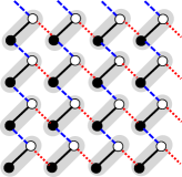
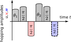
Figure 9: Left: the lattice on which the 2DQW is realized as a continuously driven Hamiltonian. Gray shaded unit cells include two sites each. The three types of hoppings allowed are intracell (black), horizontal intercell (red) and vertical intercell (blue). Right: the drive sequence for the lattice Hamiltonian.

For this continuously driven Hamiltonian, we calculate the Rudner invariant numerically, discretizing the integral of Eq. (22), and find quantized values to a great precision. The results are shown in Fig. 8. We checked numerically that these invariants correctly predict the edge states at reflective edges, and also reproduce the edge states between different bulk phases of Ref. Kitagawa, 2012.

V.3 Cut links as a bulk phase: the 4-step 2D discrete-time quantum walk

To obtain a more complete picture of the conveyor belt mechanism, it is instructive to view the line where the links are cut as the limiting case of a long thin domain of a more general quantum walk with modified parameters. To obtain this more general quantum walk, we start from the continuous-time periodically driven Hamiltonian, Eq. (24). There is a straightforward way to cut the link in the $x$ $(y)$ direction: simply omit the pulse of $v(t)$ $(w(t))$ from the sequence. This leads us to consider periodically driven systems composed of pulses of arbitrary area, as represented in Fig. 10,

$$u(t) =\left(\theta_{1}\!+\frac{\pi}{2}\right)G\Big{(}t-\frac{1}{8}\Big{)}+\left(\theta_{2}\!+\frac{\pi}{2}\right)G\Big{(}t-\frac{5}{8}\Big{)};$$ (29)

$$v(t) =\left(\phi_{1}-\frac{\pi}{2}\right)G\Big{(}t-\frac{3}{8}\Big{)};$$ (30)

$$w(t) =\left(\phi_{2}-\frac{\pi}{2}\right)G\Big{(}t-\frac{7}{8}\Big{)}.$$ (31)

We can interpret this pulse sequence as a continuous-time realization of a discrete-time quantum walk. This is the 4-step walk, defined by

$$U=S_{y}\,e^{-i\phi_{2}\sigma_{y}}\,S_{y}\,e^{-i\theta_{2}\sigma_{y}}\,S_{x}\,e^{-i\phi_{1}\sigma_{y}}\,S_{x}\,e^{-i\theta_{1}\sigma_{y}}.$$ (32)

This walk is easiest represented on a Lieb lattice, as shown in Fig. 10. At the beginning and end of each cycle, the walker is on one of the (gray) lattice sites with coordination number 4, while during the timestep, it can also occupy the (red and blue) sites with coordination number 2.

The 4-step walk has two topological invariants: the Chern number $C$, and the Rudner winding number $W$. Its Chern number can be nonzero, because at the end of the timestep the walker can also return to its starting point, and so it does not have the sublattice property detailed in the Appendix C. We find that, depending on the angles $\phi_{1},\phi_{2},\theta_{1},\theta_{2}$, the invariants can take on the values $-1,0,+1$, as shown in Fig. 11. In particular, the trivial insulator, with $C=W=0$, is realized in the areas in parameter space defined by $n\pi-\left|{\phi_{1}-\phi_{2}}\right|<\theta_{1}-\theta_{2}<n\pi+\left|{\phi_{1}-\phi_{2}}\right|$, for $n=0$ (including $U=-1$) and $n=\pm 1$ (including $U=1$). The phase with all links cut corresponds to $\theta_{1}=\theta_{2}=-\phi_{1}=-\phi_{2}=-\pi/2$; in this case, the time evolution operator does nothing to the state.

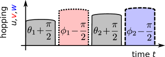
Figure 10: The 4-step quantum walk is set on a Lieb lattice (left). The driving sequence of the corresponding continuously driven Hamiltonian consists of nonoverlapping pulses of arbitrary area (right).

Figure 11: Parameter space of the 4-step 2DQW as defined in Eq. (32). Gapped domains, with Rudner winding numbers $W$ (boldface) and Chern numbers (normal typeface), are separated by lines, along which the bulk quasienergy gap around $\varepsilon=0$ (continuous lines) or around $\varepsilon=\pi$ (dotted lines) closes. Since sublattice symmetry of the walk is broken by the extra rotations through angles $\phi_{1},\phi_{2}$, the gaps can close independently, and the Chern number can take on nonzero values. The angles shown on the left are $\phi_{+}=\left|{\phi_{2}+\phi_{1}}\right|$, $\phi_{-}=\left|{\phi_{2}-\phi_{1}}\right|$, assuming both of these are less than $\pi$. In the example shown, $\phi_{1}=-\pi/10$ and $\phi_{2}=\pi/5$.

VI Robustness of the conveyor belt in the presence of disorder

We now investigate how the transport along the cut is affected by static disorder in the rotation angles $\theta_{1}$ and $\theta_{2}$, as defined in Eq. (11).

VI.1 Effects of static disorder

We choose a system of dimensions $(4M\times 2M)$. The walker is initialised at the position $A=(M,M)$. The position of the final (absorbing) point B is chosen to be $(3M-1,M-1)$. The cut cuts all the links between the sites $(x,M)$ and $(x,M-1)$ for $M\leq x\leq 3M$. Thus there is a path of cut links connecting the initial and final site. For $M=10$ the system is plotted for three different times in Fig. 12, thereby showing the initial wavefunction, the wavefunction as it propagates along the conveyor and the state after the majority of the wavefunction has been absorbed. The boundaries of the system are absorbing boundaries. This geometry is chosen such that the walker cannot reach the absorbing boundary too quickly.

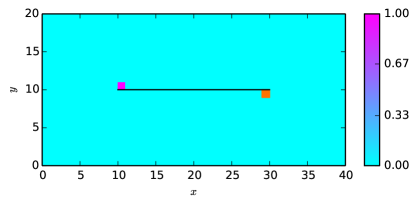
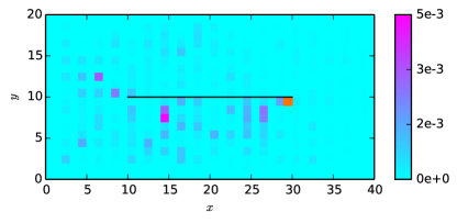
Figure 12: Wavefunction for a particular disorder realisation and the cut for a system size given by $M=10$. The values of rotation angles are $\theta_{1}=0.35\pi,\theta_{2}=0.15\pi,\delta=0.1\pi$. The cut is represented by the black line. The starting point for the wave function is just above the black line on the left. The final point at which the wave function gets absorbed is represented by the orange dot on the right-hand side. On the top plot the wave function is plotted for $t=0$. The middle plot is for $t=2M=20$ when a good fraction of the walker is on the conveyor. On the right-hand side the wave function is plotted for $t=10M=100$, long after the bulk of the walker has been absorbed by the orange point B.

We quantify the efficiency of the transport along the cut by looking at the arrival probability $P_{t}$, as in Eq. (10) and the total survival probability, i.e., the norm of the conditional wavefunction, $\langle{\Psi(t)}|{\Psi(t)}\rangle$. If these add up to 1, no part of the walker is absorbed by the boundary. If the walker is transported ballistically along the defect we expect the total arrival probability to suddenly increase by an appreciable amount at the time $t=2M/v$, where $v$ is the transport velocity of the walker, given in the clean limit by eq. (15). A delay in the onset of the arrival at the final point B indicates a slowdown of the transport. On the other hand, if the total survival probability decreases without the probability at the final point B increasing, this also indicates a loss of transport efficiency. It indicates that diffusion towards the boundary increases in importance, whereas ballistic transport along the cut decreases in importance. For different disorder strengths $\delta$ we have plotted the results of such a calculation in Fig. 13.

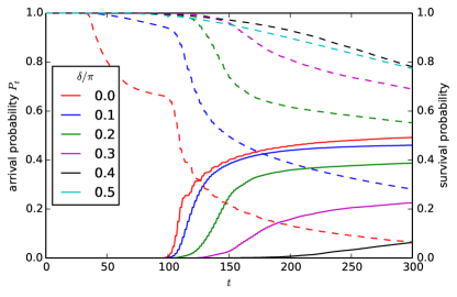
Figure 13: Top: Arrival and survival probabilities for $\theta_{1}=0.35\pi,\theta_{2}=0.15\pi$, $M=30$ and different amounts of rotation angle disorder $\delta$. Solid lines are cumulative arrival probabilities at the point B and dashed lines are the remaining wave function amplitudes, thus the probability of survival up to time $t$. The solid and dashed lines of the same colour correspond to the same system. We have averaged over 100 different disorder realisations. Bottom: Plot showing the arrival probability as a function of time for a different system sizes and different disorder strengths. The time axes is scaled with the system size. The curves for different system sizes collapse on one another, showing that the propagation along the cut is ballistic. The plot also shows that we may choose a system size of $M=30$ in order to further investigate the system.

One may obtain an overview of the behaviour as a function of $\theta_{1},\theta_{2}$ and $\delta$ by simply looking at the total survival probability and the total arrival probability for $t\gg 2M$ . Ballistically the walker should have arrived at the final point B. This allows us to see whether the transport along a conveyor is efficient for a range of parameters.

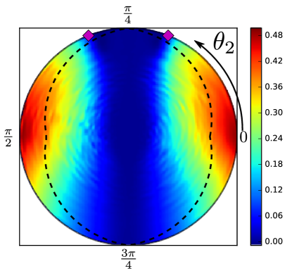
Figure 14: The arrival probability at point B after 322 time steps, averaged over 100 disorder configurations for $\theta_{1}=\frac{\pi}{4}$ as a function of $\theta_{2}$ and $\delta$. The system has the same geometry as in Fig. 12, but is three times larger, having $M=30$. In the plot the azimuthal angle represents $\theta_{2}$ and the radius is related to $\delta$ by $r=1-2\delta/\pi$, such that the largest possible value of $\delta=\pi/2$ is taken at the centre at $r=0$, at which point $\theta_{1}$ and $\theta_{2}$ are irrelevant. The black dashed line markes the regime at which $\delta$ becomes large enough for both types of topological invariants to be locally present in the system. Beyond that line transport begins to be suppressed. The magenta diamonds mark the points at which the group velocity becomes too small for the walker to arrive within the simulation time.

In Fig. 14 we have plotted the final arrival probability for $\theta_{1}=\frac{\pi}{4}$, different values of $\theta_{2}$ and a range of disorder strengths. We see that if disorder is strong enough, the ballistic transport along the defect is suppressed, and thus no part of the walker arrives at point B. A naive expectation is that disorder can start to affect the edge states only if it is large enough so that different topological invariants can be present in different parts of the system. This occurs for

$$\delta>\delta_{max}=\begin{cases}\left|{\frac{1}{2}(\theta_{2}-\pi/4)}\right|,&\theta_{2}<\frac{\pi}{2}\\ \left|{\frac{1}{2}(3\pi/4-\theta_{2}}\right|,&\theta_{2}\geq\frac{\pi}{2}\end{cases}$$ (33)

The curve $\delta_{max}(\theta)$ is plotted as the dashed black line in Fig. 14: the numerical data are more or less in agreement with the naive expectation.

The arrival probability also reduces to zero as $\theta_{2}$ approaches $\theta_{2}=\frac{\pi}{4}$ and $\theta_{2}=\frac{3\pi}{4}$, independent of the disorder. At the point $\theta_{2}=\frac{\pi}{2}$, we have $\sin(\theta_{1}-\theta_{2})=0$ and thus the group velocity along the conveyor is zero, cf. Eq. 15. Since the walker has to traverse a distance of $2M$ and the simulation time only runs up to $t_{max}$, the walker will not arrive if $v<v_{crit}=2M/t_{max}$. For Fig. 14 $v_{crit}=0.19$. From eq. (15) it then follows that the arrival probability should be zero even in the clean limit when $\theta_{2}$ is within a distance $\delta\theta_{2}^{crit}=0.06\pi$ of $\theta_{2}=\frac{\pi}{4}$. These points are marked as magenta diamonds in Fig. 14. This estimate agrees well with the position at which the arrival probability vanishes in Fig. 14.

Around the point $\theta_{2}=\frac{3\pi}{4}$ on the other hand the group velocity does not vanish. Instead, according to eq. (16) the penetration depth of the edge state into the bulk $\xi$ diverges. Thus the overlap of the initial state of the quantum walk with the conveyor vanishes, as initially the quantum walker is localised to a single lattice site. Also the overlap of the conveyor state with the final absorbing point disappears. Together with eq. (16) this implies that the arrival probability $P_{\infty}$ around $\theta_{2}=\frac{3\pi}{4}$ will vanish as

$$P_{\infty}=2\,\delta\theta_{z}^{2}$$ (34)

where $\delta\theta_{z}=\theta_{2}-\frac{3\pi}{4}$. We have numerically checked this behaviour for the clean system and find that eq. (34) provides a good fit without any adjustable parameters. So we observe qualitatively quite different behaviour around the points $\theta_{2}=\frac{\pi}{4}$ and $\theta_{2}=\frac{3\pi}{4}$. For $\theta_{2}=\frac{\pi}{4}$, $P_{\infty}$ vanishes abruptly and stays zero over a finite range of $\theta_{2}$, namely, between the two magenta diamonds in Fig. 14. On the other hand, $P_{\infty}$ vanishes gradually around $\theta_{2}=\frac{3\pi}{4}$ and is only strictly zero at one point.

VII Conclusions

In this work we have shown that in the 2-dimensional split-step discrete-time quantum walk, a cut on the underlying lattice creates a transport channel for the walker that is robust against time-independent disorder. The mechanism for the transport is given by edge states that form in the vicinity of the cut. We derived analytical formulas for some properties of the edge states, and found the bulk topological invariant that predicts their emergence. This invariant is the winding of the quasienergyRudner et al. (2013).

The edge states we found are resistant to a moderate amount time-independent disorder, but, as we have seen, above a certain threshold they no longer exist. It is an interesting challenge to study the details of this transition. In other words: how does disorder destroy the topological phase? An important step in this direction is understanding the effect of disorder on the 2DQW without edges, our results on which are published elsewhereEdge and Asboth (2014).

There are quite promising perspectives for detecting the type of edge states we found in quantum walk experiments. In fact, edge states due to the Chern numbers have already been seen in a continuous-time quantum walk experiment: there, the walker was a pulse of light coupled into an array of waveguides etched into a block of dielectric, a “photonic topological insulator”Rechtsman et al. (2013). Modifying the pattern of the waveguides would allow for a direct realization of the 2DQW. A more direct realization, which would also allow the study of interactions, would be on ultracold atoms trapped in an optical latticeGenske et al. (2013).

Appendix A Propagation around a more complicated cut

In order to illustrate that the quantum walker can also follow a cut which is not as simple as the one investigated in section III and VI, we have created a more complicated structure. This involves multiple corners and also intersections of different cuts. In Fig. 15 we investigate the propagation around a star-shaped figure, choosing as a starting point one of the corners of the star and as the endpoint another corner. We show the wave function for 6 different time slices. We can clearly see that the quantum walker propagates around the star.

Figure 15: Illustration of the conveyor mechanism around a star-shaped figure for a single disorder realisation. We have plotted the wavefunction at different times $t$, starting at $t=0$ and ending at $t=150$, at which point the majority of the wavefunction amplitude has been absorbed by the final point, marked in orange. Note that the colour scale changes between the different panels. $\theta_{1}=0.45\pi,\theta_{2}=-0.05\pi$ and $\delta=0.1\pi$ were chosen, as, according to Eq. (15), these maximise the propagation velocity along the cut. In the lowel panel we have plotted the arrival probability, which for large times approaches $P_{t}=0.7$.

Appendix B Edge State dispersion relations

In this Section we derive the edge state dispersion relations of edge states of a 2DQW below a horizontal cut, using the transfer matrix. We consider the 2DQW on a semi-infinite plane of integer lattice points, i.e., $x,y\in\mathbb{Z}$ and $y<0$, with boundary conditions given by the cut along $x$, above the line $y=0$. We assume translation invariance along $x$, i.e., along the cut. In that case the quasimomentum along $x$ is a good quantum number, we denote it by $k$. Eigenstates of the walk can be taken in a plane wave form,

$$\Psi_{k}(x,y,s)=e^{ikx}\Psi_{y}^{s},$$ (35)

with $s=\uparrow$ or $s=\downarrow$. Since the shift along $x$ can be written as $S_{x}=e^{-ik\sigma_{z}}$, the eigenvalue equation of the walk reads

$$U =S_{y}V(k);$$ (36)

$$V(k) =e^{-i\theta_{2}\sigma_{y}}e^{-ik\sigma_{z}}e^{-i\theta_{1}\sigma_{y}}.$$ (37)

Note that apart from $\text{det }V=1$, we also have

$${V^{\downarrow\downarrow}}^{\ast} =V^{\uparrow\uparrow}=c_{+}\cos k-ic_{-}\sin k;$$ (38)

$$V^{\downarrow\uparrow} =-{V^{\uparrow\downarrow}}^{\ast}=s_{+}\cos k+is_{-}\sin k,$$ (39)

where we use the shorthands

$$s_{\pm} =\sin(\theta_{1}\pm\theta_{2});$$ (40)

$$c_{\pm} =\cos(\theta_{1}\pm\theta_{2}).$$ (41)

The boundary conditions on the edge states for $y\to-\infty$ is that their wavefunctions should be normalizable. To put this into an equation, we first find a suitably defined transfer matrix. We consider an eigenstate $|{\Psi}\rangle$ of $U$ with quasienergy $\varepsilon$, for whose components we have

$$e^{-i\varepsilon}\Psi_{n+1}^{\uparrow} =V^{\uparrow\uparrow}\Psi_{n}^{\uparrow}+V^{\uparrow\downarrow}\Psi_{n}^{\downarrow};$$ (42a)

$$e^{-i\varepsilon}\Psi_{n-1}^{\downarrow} =V^{\downarrow\uparrow}\Psi_{n}^{\uparrow}+V^{\downarrow\downarrow}\Psi_{n}^{\downarrow}.$$ (42b)

The transfer matrix is defined by

$$\begin{pmatrix}\Psi_{y+1}^{\uparrow}\\ \Psi_{y}^{\downarrow}\end{pmatrix} =M(\varepsilon)\begin{pmatrix}\Psi_{y}^{\uparrow}\\ \Psi_{y-1}^{\downarrow}\end{pmatrix}.$$ (43)

Substituting into (42) gives us

$$M(\varepsilon) =\frac{\cos\varepsilon+i\sin\varepsilon\sigma_{z}+\text{Re}V^{\uparrow\downarrow}\sigma_{x}-\text{Im}V^{\uparrow\downarrow}\sigma_{y}}{V^{\downarrow\downarrow}}.$$ (44)

For the eigenstate $|{\Psi}\rangle$ to be normalizable, the vector $(\Psi_{-1}^{\uparrow},\Psi_{-2}^{\downarrow})$ must be an eigenvector of the transfer matrix $M$ with eigenvalue whose absolute value is higher than one. The eigenvalues of $M$ are

$$m_{\pm} =\frac{\cos\varepsilon\pm\sqrt{\left|{V^{\uparrow\downarrow}}\right|^{2}-\sin^{2}\varepsilon}}{V^{\downarrow\downarrow}}.$$ (45)

If $\pm\cos\varepsilon>0$, the normalizable edge state corresponds to the eigenvalue of the transfer matrix $m_{\pm}$, and we need

$$\begin{pmatrix}\Psi_{-1}^{\uparrow}\\ \Psi_{-2}^{\downarrow}\end{pmatrix} \propto\begin{pmatrix}V^{\uparrow\downarrow}\\ \pm\sqrt{\left|{V^{\uparrow\downarrow}}\right|^{2}-\sin^{2}\varepsilon}-i\sin\varepsilon\end{pmatrix}.$$ (46)

We next consider the boundary condition on the top of the ribbon, $y=0$. Here, because of the cut link, realized by $-i\sigma_{y}$, we have

$$\Psi_{0}^{\downarrow}e^{-i\varepsilon} =\left(V^{\uparrow\uparrow}\Psi_{0}^{\uparrow}+V^{\uparrow\downarrow}\Psi_{0}^{\downarrow}\right).$$ (47)

This is easiest to solve if we choose

$$\Psi_{0}^{\downarrow} =V^{\uparrow\uparrow}; \Psi_{0}^{\uparrow} =e^{-i\varepsilon}-V^{\uparrow\downarrow}.$$ (48)

Using Eqs. (42), we obtain

$$\Psi_{-1}^{\downarrow} =e^{i\varepsilon}+V^{\downarrow\uparrow}.$$ (49)

Combining the two boundary conditions, Eq. (46) with Eq. (48) and Eq. (49) above, we have

$$\frac{e^{-i\varepsilon}+{V^{\downarrow\uparrow}}^{\ast}}{e^{i\varepsilon}+V^{\downarrow\uparrow}}=\frac{-{V^{\downarrow\uparrow}}^{\ast}}{\pm\sqrt{\left|{V^{\downarrow\uparrow}}\right|^{2}-\sin^{2}\varepsilon}-i\sin\varepsilon},$$ (50)

for $\pm\cos\varepsilon>0$. The absolute values of the left-and the right-hand-side of this equation are both 1, so this is really an equation for the phases.

B.0.1 The gap around quasienergy $\varepsilon=0$

Consider $\varepsilon=0$; then Eq. (50) reads

$$\frac{1+\alpha^{\ast}}{1+\alpha} =-\frac{\alpha^{\ast}}{\left|{\alpha}\right|},$$ (51)

with

$$\alpha =s_{+}\cos k+is_{-}\sin k.$$ (52)

Solving this equation for $\text{arg}(\alpha)$, we obtain $\text{arg}\alpha=\pi$, which implies

$$k=\pi \text{ if }s_{+}>0;$$ (53)

$$k=0 \text{ if }s_{+}<0.$$ (54)

The edge state wavefunctions decay exponentially towards the bulk, as $\left|{\Psi_{y}^{s}}\right|=\left|{\Psi_{0}^{s}}\right|e^{-\left|{y}\right|/\xi}$. To obtain their penetration length for $\pm s_{+}>0$, we substitute $\cos\varepsilon=1$, $\sin k=0$, $\cos k=\pm 1$, into Eq. (45), and get

$$\xi =-\left(\text{log }\frac{1-\left|{s_{+}}\right|}{\left|{c_{+}}\right|}\right)^{-1}.$$ (55)

To obtain the group velocities, we solve Eq. (50) around $\varepsilon\approx 0$. If $s_{+}>0$ ($s_{+}<0$), then we have $k\approx 0$ ($k\approx\pi$). In both cases, if we use $k$ to denote the small distance from 0 or $\pi$, we find to 1st order in the small parameters $\varepsilon$ and $k$,

$$V^{\uparrow\downarrow} =\mp s_{+}\pm iks_{-},$$ (56)

$$\sqrt{\left|{V^{\uparrow\downarrow}}\right|^{2}-\varepsilon^{2}} =\pm s_{+}.$$ (57)

So Eq. (50) transforms to

$$\frac{1+i\varepsilon\mp s_{+}\pm iks_{-}}{1-i\varepsilon\mp s_{+}\mp iks_{-}} =\frac{\mp s_{+}\pm iks_{-}}{\mp s_{+}-i\varepsilon}.$$ (58)

To first order in the small parameters, this gives us

$$\frac{\varepsilon}{k}=\mp s_{-}$$ (59)

B.0.2 The gap around quasienergy $\varepsilon=\pi$

The edge states in the quasienergy gap around $\varepsilon=\pi$ are the sublattice partners of the edge states around $\varepsilon=0$. Due to the sublattice symmetry of the quantum walk, any eigenstate of the walk at quasienergy $\varepsilon$ with wavefunction $\Psi(x,y)$ has a sublattice partner with quasienergy $\varepsilon+\pi$ and wavefunction

$$\Gamma\Psi(x,y)=e^{i\pi x}e^{i\pi y}\Psi(x,y).$$ (60)

Thus, for a fixed value of the rotation angle parameters $\theta_{1}$ and $\theta_{2}$, edge states in the gap at $\varepsilon\approx\pi$ have the same penetration depth and group velocity as those at $\varepsilon\approx 0$, and are around $k=\pi$ ($k=0$) when those in the gap around $\varepsilon=0$ are around $k=0$ ($k=\pi$).

B.0.3 Summary: group velocity and penetration depth

To summarize, at the middle of both of the gaps around $\varepsilon=0$ and $\varepsilon=\pi$, the edge states have the group velocity

$$\frac{d\varepsilon}{dk} =\text{sign}(\theta_{1}+\theta_{2})\sin(\theta_{2}-\theta_{1}),$$ (61)

and penetration depth

$$\xi =-\left(\text{log }\frac{1-\left|{\sin(\theta_{1}+\theta_{2}}\right|}{\left|{\cos(\theta_{1}-\theta_{2})}\right|}\right)^{-1}.$$ (62)

Appendix C Sublattice symmetry of a Quantum Walk and Chern numbers

To understand the sublattice symmetry of the split-step quantum walk, assign each site on the lattice one of four sublattice indices,

$$f(x,y)=2(y\text{ mod }2)+(x+y)\text{ mod }2,$$ (63)

and use the corresponding sublattice projection operators,

$$\Pi_{j}=\sum_{x,y:f(x,y)=j}|{x,y}\rangle\langle{x,y}|,$$ (64)

where $j\in\{0,1,2,3\}$. One timestep $U$ changes the sublattice index by $2$, as can be checked explicitly. Thus, a walker started at $x_{0},y_{0}$ on sublattice $j$ will be on sublattice $j+2\text{ mod }2$ after an odd number of timesteps, and return to sublattice $j$ after an even number of timesteps. Now define the sublattice operator $\Gamma$ as

$$\Gamma =\Pi_{0}+\Pi_{2}-\Pi_{1}-\Pi_{3}.$$ (65)

This operator acts on a wavefunction $\Psi(x,y)$ as

$$\Gamma\Psi(x,y)=e^{i\pi x}e^{i\pi y}\Psi(x,y).$$ (66)

When acting on a plane wave, $\Gamma$ shifts its wavenumber by $(\pi,\pi)$. On the other hand, acting on an eigenstate of the walk, it shifts the quasienergy by $\pi$, since

$$\Gamma U\Gamma =-U \to\quad\Gamma H_{\text{eff}}\Gamma=H_{\text{eff}}+\pi.$$ (67)

This means that every band with Chern number $C$ has a sublattice symmetric partner that is shifted in energy by $\pi$ with the same Chern number $C$. Since the sum of all Chern numbers have to be 0, in a two-band model, such as the split-step walk, this precludes the existence of a band with a nonzero Chern number.