Detecting nonlocal Cooper pair entanglement by optical Bell inequality violation

Abstract

Based on the Bardeen Cooper Schrieffer (BCS) theory of superconductivity, the coherent splitting of Cooper pairs from a superconductor to two spatially separated quantum dots has been predicted to generate nonlocal pairs of entangled electrons. In order to test this hypothesis, we propose a scheme to transfer the spin state of a split Cooper pair onto the polarization state of a pair of optical photons. We show that the produced photon pairs can be used to violate a Bell inequality, unambiguously demonstrating the entanglement of the split Cooper pairs.

I Introduction

Entanglement Schrödinger (1935), i.e., correlations between parts of a quantum system that defy any classical description, lies at the heart of quantum mechanics. It is the basis for many applications of quantum information theory, such as quantum teleportation Bouwmeester et al. (1997), quantum computing Jozsa and Linden (2003), quantum cryptography Jennewein et al. (2000), and quantum metrology Giovannetti et al. (2011). The first experimental demonstration of entanglement has been achieved by violating Bell’s inequality Bell (1964) with polarization-entangled optical photon pairs generated during spontaneous parametric down-conversion in a nonlinear crystal Aspect et al. (1982). In many applications, it is desirable to have a source of entangled pairs of spatially separated particles. Such pairs are called EPR pairs in reference to the seminal work of Einstein, Podolsky and Rosen on the completeness of quantum mechanics Einstein et al. (1935).

Compared to quantum optical scenarios, the generation of electronic EPR pairs is rather challenging. EPR pairs of electrons are nonetheless highly desirable because an on-demand generation of such pairs would facilitate certain quantum communication tasks in solid-state devices Bennett and DiVincenzo (2000). Theoretically, a conventional $s$-wave superconductor provides a natural source for electronic EPR pairs Choi et al. (2000); Recher et al. (2001); Lesovik et al. (2001); Hofstetter et al. (2009); Herrmann et al. (2010); Das et al. (2012); Cottet et al. (2012); Braunecker et al. (2013); Cottet (2014): the electrons in a BCS superconductor form spin singlet Cooper pairs in the ground state. Following theoretical proposals Recher et al. (2001); Lesovik et al. (2001), the coherent splitting of Cooper pairs, originating from a superconducting electrode, into two spatially separated electrons on neighboring quantum dots (QDs) has recently been demonstrated experimentally Hofstetter et al. (2009); Herrmann et al. (2010); Das et al. (2012). While measurements of the current flowing out of the QDs have indeed demonstrated the splitting of Cooper pairs, the detection of the spin entanglement of the expected electronic singlet state has so far remained elusive. Similar devices can be used as a tool to detect unconventional pairing in superconductors Tiwari et al. (2012) or to entangle mechanical resonators Walter et al. (2012).

Detecting the entanglement of electronic EPR pairs is not as straightforward as it is with their counterparts in quantum optics. Several works Kawabata (2001); Chtchelkatchev et al. (2002); Braunecker et al. (2013); Scherübl et al. (2014) propose to violate a Bell-type inequality with current noise measurements. However, this will require accurate measurements of the cross-correlations between the currents from the two QDs. A measurable signal only emerges if these currents are large enough, i.e., for a strong coupling of the QDs to the measurement device (“open quantum dots”). This conflicts with the requirement of isolating the QDs from the environment (“closed quantum dots”), which is necessary for splitting Cooper pairs coherently in the first place. Moreover, most existing proposals involve the use of strong ferromagnets and complex sample geometries, and neglect (possibly long-range) electron-electron interactions when computing the current-current correlations. As shown in Ref. Burkard et al. (2000), such interactions can reduce the measured entanglement signal. Another approach, which is closest in spirit to our work, is taken in Veronica Cerletti, Oliver Gywat, and Daniel Loss (2005); Jan Budich and Björn Trauzettel (2010). These authors investigate the possibility to transfer electron spin entanglement to photon polarization states. These particular schemes however, suffer from a low detection efficiency and require the use of additional quantum resources to generate a pure two-photon state footnote . Very recently, the possibility of generating polarization entangled photons in a superconducting p-n junction has been proposed Schroer (2014).

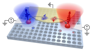
Figure 1: Schematics of a possible realization of the entanglement transfer scheme. The perforated blue slab represents a photonic crystal with two cavities (central areas without holes). Photons in each cavity are coupled to the respective QDs (red domes) via electric dipole interactions. The QDs are tunnel coupled to a superconductor (yellow half-disc on top). Gates (gray slabs) allow for tuning of the QD chemical potentials. The emission cones of the entangled photons are depicted as red and blue shades.

Our proposal avoids the above difficulties by converting the spin entanglement of a single Cooper pair into polarization entanglement of a single pair of optical photons and requires only classical resources such as laser drives and tunable gate voltages. Because photons do not interact with each other, photonic entanglement is more robust to perturbations than electronic entanglement, and can be detected using standard Bell-type measurements. Provided sufficiently independent cavities are used (See Appendix. F and Ref. Brossard et all. (2013)), there can be no doubt that the entanglement ultimately measured stems from the split Cooper pair because our entanglement transfer scheme involves only local operations. Since our scheme does not involve the measurement of electronic currents, it works even in closed QDs. Finally, we show that the entanglement transfer can be carried out on time scales small compared to $T_{2}$, the intrinsic coherence time of the QDs (see Appendix G).

II Setup

Let us first present our proposed experimental setup in more detail. A schematic drawing of a possible realization is shown in Fig. 1. Our starting point is the typical setup for Cooper pair splitters, i.e., a superconductor which is tunnel coupled to two nearby QDs Recher et al. (2001). The spacing between the QDs should be smaller than the superconducting coherence length and the QDs are assumed to be in the Coulomb blockade regime such that adding an electron to the QDs requires a large charging energy $U$. The onsite energies of the QDs can be tuned via gate voltages. Splitting a Cooper pair into a singlet state shared between the two QDs becomes energetically possible if the total energy of the singlet state coincides with the chemical potential of the superconductor. Both QDs are embedded into optical cavities that serve as frequency filters allowing only certain desired optical transitions. The small distance between the QDs rules out conventional optical cavities, but photonic crystal cavities are nowadays easy to manufacture at the required length scales and can have optical linewidths and frequencies compatible with our proposal Yoshie et al. (2004). Moreover, cavities with high quality factors and directional out-coupling of photons into a narrow solid angle for high-efficiency collection have been fabricated Kim et al. (2004); Tran et al. (2009); Portalupi et al. (2010) and self-assembled QDs have been successfully embedded into photonic crystals in several experiments Yoshie et al. (2004); Majumdar et al. (2013); Sweeney et al. (2014).

III Entanglement transfer scheme

We will now present our scheme for transferring the spin entanglement of a Cooper pair onto the polarization state of a photon pair. For simplicity, we discuss a left-right symmetric setup. To be specific, we assume that the QDs are realized as self-assembled GaAs QDs. The relevant electronic levels are thus generated from the light-hole (lh) and heavy-hole (hh) bands forming the valence band, as well as the conduction band (cb). The energy difference between the hole bands $\Delta E=E^{{\text{hh}}}-E^{{\text{lh}}}$ is of the same order as the superconducting gap $\Delta$, whereas the transition frequency between the valence band and the conduction band is in the optical frequency range Gywat et al. (2010). Moreover, we assume that a weak magnetic field is applied which causes a Zeeman splitting $\Delta_{Z}$ (with $|\Delta_{Z}|\ll\Delta,\Delta E$) of all electronic levels.

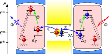
Figure 2: Level diagram and schematics of the three phases of the entanglement transfer. The lowest light-hole states $\left|{{\text{lh}},\downarrow}\right\rangle_{L,R}$ are occupied and transitions into them are forbidden because of the Pauli principle (hash marks).

The entanglement transfer can be split into initialization and three phases, which we discuss next. A schematic level diagram along with the essential steps of our scheme is shown in Fig. 2.

Initialization: Initially, the gate voltages of the QDs are tuned in such a way that the lowest light-hole states on each QD, $\left|{{\text{lh}},\downarrow}\right\rangle_{L}$ and $\left|{{\text{lh}},\downarrow}\right\rangle_{R}$, are occupied. Furthermore the heavy-hole level resides in the superconducting gap but is detuned with respect to the chemical potential of the superconductor.

Phase 1: The splitting of a Cooper pair is achieved by tuning the gate voltages to bring the heavy-hole level into resonance with the chemical potential of the superconductor. Single-particle tunneling is suppressed due to the large superconducting gap. Furthermore, the large onsite Coulomb interaction in the QD suppresses the tunneling of both electrons of a Cooper pair onto the same QD. The Cooper pair splitting process, where one electron tunnels to each QD, is thus the dominant process Recher et al. (2001). When the separation between the QDs is much smaller than the superconducting coherence length, the Cooper pair splitting rate is (see Appendix A) $\hbar\Gamma_{c}\approx\pi\rho_{0}w_{L}w_{R}[1-(\Delta_{Z}/2\Delta)^{2}]^{-1/2}$. Here, $w_{L}$ ($w_{R}$) denotes the electronic tunnel amplitude between the superconductor and the left (right) QD and $\rho_{0}$ denotes the normal-state density of states of the superconductor. If $\Gamma_{c}\gg 1/T_{2}$, where $T_{2}$ is the intrinsic coherence time of the QDs, this process is coherent and leads to Rabi oscillations between the superconductor and the heavy-hole states on the QDs. Ideally, after half a period, the double-QD is occupied by a singlet state and the oscillation is stopped by detuning the heavy-hole level away from resonance.

Phase 2: Next, the electrons in the QDs are excited from the heavy-hole to the conduction band. This is achieved by switching on a strong drive laser on each of the two QDs, with frequency $\hbar\omega_{\rm drive}\approx E^{{\text{cb}}}-E^{{\text{hh}}}$. A linearly polarized drive can be used, which induces spin conserving transitions. After half a Rabi period the laser is switched off, having lifted the singlet state into the conduction band levels. If the Zeeman splittings of the heavy hole and conduction bands differ, one may use two drive lasers per QD to satisfy the resonance conditions for the two different transition frequencies simultaneously. The duration of this step is inversely proportional to the drive strength and can thus be made fast compared with $T_{2}$.

Phase 3: The resonance frequencies of the two optical cavities are chosen to be close to the transition frequency between the conduction band and the light-hole band, $\hbar\omega_{\rm cav}\approx E^{{\text{cb}}}-E^{{\text{lh}}}$. Furthermore, the cavity linewidth $\kappa$ is assumed to be much smaller than the frequency separation between the light- and heavy-hole bands, i.e., $\kappa\ll(E^{{\text{hh}}}-E^{{\text{lh}}})/\hbar$. Therefore, the decay of the conduction band electrons into the light-hole band due to the dipole coupling of strength $\hbar g$ between electrons and photons, will be strongly enhanced, whereas the decay into heavy-hole states is suppressed. Since the lowest light-hole state $\left|{{\text{lh}},\downarrow}\right\rangle$ is always occupied, a conduction band electron in the states $\left|{{\text{cb}},\uparrow}\right\rangle$ or $\left|{{\text{cb}},\downarrow}\right\rangle$ can only transition to the empty $\left|{{\text{lh}},\uparrow}\right\rangle$ state via the emission of a linearly or circularly polarized photon, respectively.

To investigate these three phases, we have numerically solved the Schrödinger equation for the full system in the coherent limit $\kappa\rightarrow 0$ (see Appendix B). Figure 3 shows the evolution during each phase of the occupation of the electronic levels and the cavity mode for an optimal choice of the drive strengths and drive durations. In the limit $\kappa\to 0$, the emitted photons undergo coherent oscillations between the QD and the cavity. Ideally, after half a Rabi period $\approx\pi/(2g)$, the electrons in both QDs occupy the $\left|{{\text{lh}},\uparrow}\right\rangle$ states while the electronic entanglement has been transferred to the photons.

IV Photon extraction and Bell test

In a real experiment, the photons need to be extracted from the cavities for measurement. This is achieved by coupling each cavity to a continuum of modes, e.g., as provided by a waveguide. Hence, the cavity acquires a finite loss rate $\kappa>0$. As discussed further below, we will focus on the weak coupling limit, where $g\ll\kappa$. In this limit, the coherent oscillations are suppressed and the photons are emitted into the continuum on a time scale $\propto\kappa/g^{2}$.

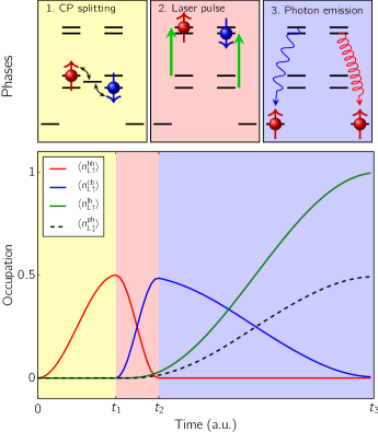
Figure 3: Upper panel: Schematics of the three phases showing Cooper pair splitting in phase one, laser-driven spin-conserving transitions populating the conduction band states in phase two, and emission of entangled photons into the cavities in phase three. Lower panel: Numerically calculated time evolution, in the coherent limit $\kappa\rightarrow 0$, of the occupation probability of various electronic and photonic modes. At the end of phase one, marked by $t_{1}=\pi/2\Gamma_{c}$, the electronic occupation per spin in the heavy-hole band reaches its maximum ($\approx 0.5$). During phase two, between $t_{1}$ and $t_{2}$, the electronic population is transferred from the heavy-hole band to the conduction band. Once the conduction band is occupied the electrons can transition from the conduction band to the light-hole band by emitting photons into the cavity. At the end of phase three, marked by $t_{3}$, the electronic system is in the product state $\left|{\psi}\right\rangle_{\rm el}\approx\left|{{\text{lh}},\uparrow}\right\rangle_{L}\left|{{\text{lh}},\uparrow}\right\rangle_{R}$, and the entanglement has been transferred to the photonic degree of freedom (see text and Fig. 6).

Once both photons have been emitted, the electronic singlet has been transferred onto a two-photon state, ideally given by

$$\left|{\psi}\right\rangle_{\rm ph}=\mathcal{N}\left(\left|{\omega_{\updownarrow},\updownarrow}\right\rangle_{L}\left|{\omega_{\circlearrowleft},\circlearrowleft}\right\rangle_{R}-\left|{\omega_{\circlearrowleft},\circlearrowleft}\right\rangle_{L}\left|{\omega_{\updownarrow},\updownarrow}\right\rangle_{R}\right).$$ (1)

Here $|{\omega_{p},p}\rangle$, with $p\in\{\updownarrow,\circlearrowleft\}$, represents the photon states emitted into the continuum modes with either linear ($\updownarrow$) or circular ($\circlearrowleft$) polarization, and $\omega_{p}$ denotes the corresponding transition frequency. Importantly, because of the finite linewidth of the electronic levels, the emitted photons are spread out in frequency. Let us characterize the frequency overlap by $\varepsilon=1-|\left\langle{\omega_{\updownarrow}|\omega_{\circlearrowleft}}\right\rangle|^{2}$. The normalization of the above photonic state $\left|{\psi}\right\rangle_{\rm ph}$ is then given by $\mathcal{N}=(1+\varepsilon)^{-1/2}$. As we show next, the entanglement of the state (1) can be detected by standard polarization measurements, as long as $\varepsilon$ is below a certain threshold value.

The density matrix of the polarization degree of freedom is obtained by tracing $\rho_{\rm ph}=\left|{\psi}\right\rangle\left<{\psi}\right|_{\rm ph}$ in Eq. (1) over the frequency degree of freedom,

$$\rho_{\rm pol} =\frac{1}{1+\varepsilon}\Big{[}\left|{\updownarrow,\circlearrowleft}\right\rangle\left<{\updownarrow,\circlearrowleft}\right|+\left|{\circlearrowleft,\updownarrow}\right\rangle\left<{\circlearrowleft,\updownarrow}\right|$$

$$\phantom{=\frac{1}{1+\varepsilon}\Big{(}}-(1-\varepsilon)\left(\left|{\updownarrow,\circlearrowleft}\right\rangle\left<{\circlearrowleft,\updownarrow}\right|+\text{h.c.}\right)\Big{]},$$ (2)

where we have introduced the shorthand notation $\left|{\updownarrow,\circlearrowleft}\right\rangle\equiv\left|{\updownarrow}\right\rangle_{L}\otimes\left|{\circlearrowleft}\right\rangle_{R}$ and similar for the other two-photon polarization states. In the limit $\varepsilon\rightarrow 1$, corresponding to distinguishable frequencies, the state (IV) is separable: $\rho_{\rm pol}=\big{(}\rho_{\updownarrow}^{(L)}\otimes\rho_{\circlearrowleft}^{(R)}+\rho_{\circlearrowleft}^{(L)}\otimes\rho_{\updownarrow}^{(R)}\big{)}/2$ with $\rho_{p}^{(\alpha)}=\left|{p}\right\rangle\left<{p}\right|_{\alpha}$. In the other limit $\varepsilon\rightarrow 0$, corresponding to indistinguishable frequencies, the state (IV) is maximally entangled: $\rho_{\rm pol}=\left|{\psi_{-}}\right\rangle\left<{\psi_{-}}\right|$ with $\left|{\psi_{-}}\right\rangle=\big{(}\left|{\updownarrow,\leftrightarrow}\right\rangle-\left|{\leftrightarrow,\updownarrow}\right\rangle\big{)}/\sqrt{2}$. To obtain the latter expression, we have decomposed the circularly polarized state as a superposition of two orthogonal linearly polarized states $\left|{\circlearrowleft}\right\rangle=(\left|{\updownarrow}\right\rangle+i\left|{\leftrightarrow}\right\rangle)/\sqrt{2}$. Thus, depending on the value of $\varepsilon$, the polarization degree of freedom may or may not be entangled.

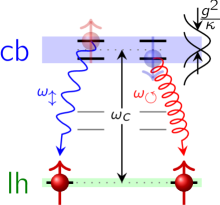
Figure 4: Schematics of the level scheme relevant for the frequency disentangling Purcell emission process. We omit the filled lower lh states because transitions to the latter are blocked (see text).

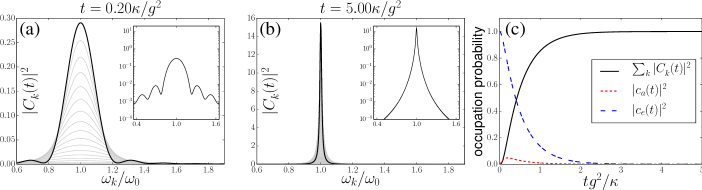
Figure 5: Panels (a) and (b): Snapshots of the frequency distribution of the emitted photon. At short time $t\ll\kappa/g^{2}$, transient coherent oscillations are clearly visible in the logarithmic plot shown in the inset (a) and are suppressed at long time $t\gg\kappa/g^{2}$, when the distribution becomes Lorentzian (b). Panel (c): Evolution of the occupation probabilities of electronic state, cavity mode and integrated continuum modes. Note that the cavity population $|c_{a}(t)|^{2}$ remains small at all time.

An experimentally accessible way of demonstrating entanglement in polarization is provided by the violation of the Clauser-Horne-Shimony-Holt (CHSH) variant of Bell’s inequality Clauser et al. (1969); by now a standard technique of quantum optics Aspect et al. (1982). In our case, we find that $\rho_{\rm pol}$ violates the CHSH inequality if (see Appendix C)

$$\varepsilon<\frac{\sqrt{2}-1}{\sqrt{2}+1}.$$ (3)

To relate $\varepsilon$ with the parameters of our model, we use the Weisskopf-Wigner (WW) theory Weisskopf and Wigner (1930) of the Purcell effect, which allows us to derive analytically the state of the photons emitted into the continuum by the electronic system via the cavity.

The relevant part of the level scheme is depicted in Fig. 4. We consider the zero-temperature limit where the cavity is initially empty. In each QD, the problem then separates into two independent Purcell emission processes, corresponding to transitions from the conduction band levels $\left|{{\text{cb}},\uparrow}\right\rangle$ and $\left|{{\text{cb}},\downarrow}\right\rangle$ into the unoccupied light-hole state $\left|{{\text{lh}},\uparrow}\right\rangle$ (blue and red arrows in Fig. 4). For each of these transitions, the photon emission process can be described by the Jaynes-Cummings Hamiltonian Jaynes and Cummings (1963), where the cavity mode is coupled to a bosonic quasi-continuum. Within the WW theory, the associated Schrödinger equation can be solved analytically (see Appendix D) and the solution is given by

$$\left|{\psi}\right\rangle=c_{e}\left|{1,0,\{0\}}\right\rangle+c_{a}\left|{0,1,\{0\}}\right\rangle+\sum_{k}C_{k}\left|{0,0,\{1_{k}\}}\right\rangle.$$ (4)

Here $\left|{n,m,\{s_{k}\}}\right\rangle$ denotes a state with $n$ electrons in the conduction band level, $m$ photons in the cavity mode and $s_{k}$ photons with momentum $k$ in the continuum ($\left|{\{0\}}\right\rangle$ denotes the vacuum state of the continuum). Since we want to extract the photons quickly and avoid coherent oscillations between the cavity and the electrons, we focus on the weak-coupling, near-resonant regime where $g,|\delta|\ll\kappa$. Here $\delta=\omega_{\rm cav}-\omega_{0}$ is the detuning of the cavity mode $\omega_{\rm cav}$ from the spin-conserving and spin-flipping electronic transitions with frequencies $\omega_{0}=\omega_{\updownarrow}=(E^{{\text{cb}}}_{\uparrow}-E^{{\text{lh}}}_{\uparrow})/\hbar$ and $\omega_{0}=\omega_{\circlearrowleft}=(E^{{\text{cb}}}_{\downarrow}-E^{{\text{lh}}}_{\uparrow})/\hbar$, respectively.

At long time $t\gg\kappa/g^{2}$, $c_{e}(t)$ and $c_{a}(t)$ vanish (see Fig. 5, panel (c)), while the amplitude of the emitted photon $C_{k}(t)$ asymptotically goes towards (see Fig. 5 panels (a) and (b) and Appendix D)

$$C_{k}(t\gg\kappa/g^{2})\approx\frac{-\nu_{0}ge^{-i\omega_{k}t}}{\left(\kappa_{0}+i(\omega_{0}-\omega_{k})\right)\left(\kappa_{c}+i(\omega_{\rm cav}-\omega_{k})\right)},$$ (5)

where $\kappa_{0}\approx g^{2}/\kappa$, $\kappa_{c}\approx\kappa-g^{2}/\kappa$, $\omega_{k}$ is the photon frequency in the continuum, and $\nu_{0}$ is the coupling constant between the cavity mode and the continuum. The state of the emitted photon can be written as

$$\left|{\omega_{0}}\right\rangle=\sum_{k}C_{k}(t)\left|{\{1_{k}\}}\right\rangle.$$ (6)

In the long time limit, the distribution of the emitted photons is centered on the frequency $\omega_{0}$ and its width is determined by the Purcell rate $\kappa_{0}$, because this is the smaller of the two rates $\kappa_{c}$ and $\kappa_{0}$.

Equation (5) allows us to evaluate the overlap in frequency of two photons emitted during the spin-conserving and spin-flipping transitions. For $\Delta_{Z}\ll\kappa_{0}$, we can expand to leading order in $|\omega_{\updownarrow}-\omega_{\circlearrowleft}|/\kappa_{0}$ and find

$$\varepsilon=1-\left|\langle{\omega_{\updownarrow}\big{|}\omega_{\circlearrowleft}}\rangle\right|^{2} =1-\Big{|}\sum_{k}(C^{\updownarrow}_{k})^{*}C^{\circlearrowleft}_{k}\Big{|}^{2}\approx\left(\frac{\omega_{\updownarrow}-\omega_{\circlearrowleft}}{2\kappa_{0}}\right)^{2}.$$ (7)

Hence, from Eqs. (3) and (7), we find that the state of the emitted photons is entangled in polarization if

$$\frac{\left|\omega_{\updownarrow}-\omega_{\circlearrowleft}\right|}{g^{2}/\kappa}<2\left(\sqrt{2}-1\right)\approx 0.83.$$ (8)

Thus, if the linewidth of the conduction band levels induced by the Purcell effect is larger than the Zeeman splitting of the conduction band doublet, it is possible to violate Bell’s inequality, thereby demonstrating the entanglement of the split Cooper pair.

V Sensitivity to imperfections

So far we have discussed the ideal case without any imperfections. To quantify the sensitivity of the proposed scheme to realistic parameter variations, we use the numerical simulations for the coherent system ($\kappa\rightarrow 0$). In this case, the irreversible Purcell emission in phase three is replaced by coherent Rabi oscillations between the electronic system and the cavity (see Fig. 3). After half-integer multiples of the Rabi period, the photonic state in the cavities is ideally given by Eq. (1). The fidelity of the actually generated photonic state computed numerically with this ideal state is shown in the top panel of Fig. 6. To quantify the entanglement of the photonic state generated in the cavity, we compute its logarithmic negativity Vidal and Werner (2002). This is shown in the bottom panel of Fig. 6. Both the fidelity and the logarithmic negativity are shown as a function of the asymmetry of the electron-photon coupling strengths for the two polarizations $g_{\circlearrowleft}/g_{\updownarrow}$ and as a function of the detuning $\delta E^{{\text{lh}}}$ between the cavity mode and the electronic transition frequency between conduction band and light-hole band. We stress that since only local unitary operations are applied to each QD, the positivity of the logarithmic negativity of the photonic state bears witness to the entanglement of the split Cooper pair. As expected, the optimal entanglement transfer takes place closest to resonance and for equal coupling strengths. However, sizeable and detectable photon entanglement remains even away from the optimal point. In Appendix E, we further show that photonic entanglement persists even in the presence of finite electronic decoherence. Finite temperature effects are not included in the present work but could be an interesting topic for future investigation.

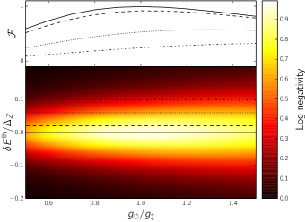
Figure 6: Upper panel: Fidelity $\mathcal{F}=\langle{\psi|\rho_{\rm ph}|\psi}\rangle_{\rm ph}$ of the numerically computed photonic state $\rho_{\rm ph}$ with the ideal state $\left|{\psi}\right\rangle_{\rm ph}$ of Eq. (1). Lower panel: Logarithmic negativity of $\rho_{\rm ph}$ as a function of photon coupling asymmetry $g_{\circlearrowleft}/g_{\updownarrow}$ and detuning $\delta E^{{\text{lh}}}=\hbar\omega_{\updownarrow}-(E^{{\text{cb}}}-E^{{\text{lh}}})$ between the cavity resonance and the electronic transition frequency. The larger the value of the logarithmic negativity, the more entanglement is present.

VI Conclusion

In conclusion, we have proposed a hybrid electro-optical scheme to detect entanglement of split Cooper pairs. By mapping the spin entanglement of electrons to the polarization entanglement of optical photons, we avoid several difficulties of previous proposals. Provided cavities with little cross-talk at a distance smaller than the superconducting coherence length can be fabricated Brossard et all. (2013) (see also Appendix F), our scheme could be implemented by combining state-of-the-art technologies: a photonic crystal cavity with coupling strength $g\approx 20\text{ GHz}$ Yoshie et al. (2004) and linewidth $\kappa\approx 100\text{ GHz}$ leads to $g^{2}/\kappa\approx 4\text{ GHz}$. This exceeds the Zeeman splitting $\Delta_{Z}\approx 0.1\text{ GHz}$ corresponding to a magnetic field of $10\text{ mT}$. With a typical Cooper pair splitting rate of $\Gamma_{c}\approx 2\text{ GHz}$ Herrmann et al. (2010), the entire entanglement transfer can thus be performed fast compared to typical decoherence rates, $1/T_{2}\approx 0.01\text{ GHz}$ Kloeffel and Loss (2013). Our scheme can thus be used to verify the entanglement-preserving nature of the Cooper pair splitting process Hofstetter et al. (2009); a crucial step towards realizing a reliable source of electronic EPR pairs in the solid state.

We would like to acknowledge stimulating discussions with Christoph Bruder. This work was financially supported by the Swiss SNF and the NCCR Quantum Science and Technology. SW acknowledges support from the ITN cQOM. TLS is supported by the National Research Fund, Luxembourg (ATTRACT 7556175).

Appendix A Effective Hamiltonian for Cooper pair splitting

In this appendix, we present a systematic derivation of the Cooper pair tunneling rate using the Schrieffer-Wolff (SW) transformation. The system under investigation is described by the Hamiltonian $H=H_{\rm SC}+H_{L}+H_{R}+K_{{\rm SC}-{\rm QD}}$, where

$$H_{\rm SC}=\sum_{{\bf k}\sigma}E_{{\bf k}}\gamma_{{\bf k}\sigma}^{\dagger}\gamma_{{\bf k}\sigma}$$ (9)

describes a conventional BCS superconductor. Here, $\gamma_{{\bf k}\sigma}$ is the quasiparticle annihilation operator (with momentum $\bf k$ and spin $\sigma\in\{\uparrow,\downarrow\}$), which is defined by $\gamma_{{\bf k}\sigma}\left|{\rm BCS}\right\rangle=0$, where $\left|{\rm BCS}\right\rangle$ denotes the BCS ground state. The quasiparticle energies are given by $E_{{\bf k}}=\sqrt{\xi_{{\bf k}}^{2}+\Delta^{2}}$, where $\Delta$ is the superconducting gap and $\xi_{{\bf k}}$ is the normal-state single-electron energy as measured from the chemical potential of the superconductor (henceforth set to zero).

Only the electronic states in the heavy-hole (hh) band of the quantum dots are included in the derivation of the Cooper pair tunneling rate. States in the light-hole and conduction bands can be safely ignored due to their larger detuning from the superconductor’s chemical potential. The Hamiltonian describing the quantum dots is

$$H_{\alpha}=\sum_{\sigma}\left(E^{({\text{hh}})}+\sigma\frac{\Delta_{Z}}{2}\right)n_{\alpha\sigma}^{({\text{hh}})},$$ (10)

where $\sigma\in\{\uparrow,\downarrow\}=\{+,-\}$ and $\alpha\in\{L,R\}$ denotes the left and right quantum dots, respectively. Moreover, $n_{\alpha\sigma}^{({\text{hh}})}=c_{\alpha\sigma}^{({\text{hh}})\dagger}c_{\alpha\sigma}^{({\text{hh}})}$ is the corresponding number operator given in terms of the electronic creation ($c_{\alpha\sigma}^{({\text{hh}})\dagger}$) and annihilation ($c_{\alpha\sigma}^{({\text{hh}})}$) operators for the electrons in the heavy-hole bands. For simplicity, we have assumed that the left and right quantum dots have the same orbital and Zeeman energies. Furthermore, the quantum dots are assumed to be in the Coulomb blockade regime, so double occupancy of the heavy-hole bands is forbidden. The tunnel coupling between the superconductor and the quantum dots is described by

$$K_{{\rm SC}-{\rm QD}}=\sum_{\sigma}\sum_{\alpha}w_{\alpha}\left(c_{\alpha\sigma}^{({\text{hh}})}\psi_{\sigma}^{\dagger}({\bf r}_{\alpha})+\text{h.c.}\right),$$ (11)

where $w_{\alpha}$ is the corresponding electron tunneling amplitude and $\psi_{\sigma}^{\dagger}({\bf r}_{\alpha})$ creates an electron (with spin $\sigma$) at position ${\bf r}_{\alpha}$ in the superconductor. Going to momentum space, we can express the tunnel coupling in terms of the electron creation ($d_{{\bf k}\sigma}^{\dagger}$) and annihilation ($d_{{\bf k}\sigma}$) operators for the superconductor, which are related to the quasiparticle operators via the Bogoliubov transformation

$$d_{{\bf k}\uparrow} = u_{{\bf k}}\gamma_{{\bf k}\uparrow}+v_{{\bf k}}\gamma_{-{\bf k}\downarrow}^{\dagger},$$

$$d_{-{\bf k}\downarrow} = u_{{\bf k}}\gamma_{-{\bf k}\downarrow}-v_{{\bf k}}\gamma_{{\bf k}\uparrow}^{\dagger}.$$ (12)

Here, $u_{{\bf k}}=(1/\sqrt{2})\sqrt{1+\xi_{{\bf k}}/E_{{\bf k}}}$ and $v_{{\bf k}}=(1/\sqrt{2})\sqrt{1-\xi_{{\bf k}}/E_{{\bf k}}}$ are the usual BCS coefficients.

We express the original Hamiltonian as $H=H_{0}+K_{\rm{SC}-\rm{QD}}$. We wish to determine a unitary transformation $\mathcal{U}=e^{-S}$ that eliminates $K_{{\rm SC}-{\rm QD}}$ to linear order in $w_{\alpha}$. Choosing the anti-Hermitian operator $S\sim\mathcal{O}(w_{\alpha})$ such that

$$[H_{0},S]=-K_{{\rm SC}-{\rm QD}},$$ (13)

the transformed Hamiltonian becomes, to second order in $w_{\alpha}/\Delta$

$$H_{\rm SW}=e^{-S}He^{S}\approx H_{0}+\frac{1}{2}[K_{{\rm SC}-{\rm QD}},S]+\mathcal{O}(w_{\alpha}^{3}).$$ (14)

The solution of (13) is given by

$$S=\sum_{\alpha}\sum_{{\bf k}\sigma}\left(\gamma_{{\bf k}\sigma}X^{\alpha}_{{\bf k}\sigma}-\text{h.c.}\right),$$ (15)

where

$$X^{\alpha}_{{\bf k}\uparrow} = w_{\alpha}\left(\frac{u_{\bf k}e^{i{\bf k}\cdot{\bf r}_{\alpha}}c^{({\text{hh}})\dagger}_{\alpha\uparrow}}{E_{{\bf k}}-E^{({\text{hh}})}-\frac{\Delta_{Z}}{2}}+\frac{v_{\bf k}^{\ast}e^{i{\bf k}\cdot{\bf r}_{\alpha}}c^{({\text{hh}})}_{\alpha\downarrow}}{E_{{\bf k}}+E^{({\text{hh}})}-\frac{\Delta_{Z}}{2}}\right)$$

$$X^{\alpha}_{{\bf k}\downarrow} = w_{\alpha}\left(\frac{u_{\bf k}e^{i{\bf k}\cdot{\bf r}_{\alpha}}c^{({\text{hh}})\dagger}_{\alpha\downarrow}}{E_{{\bf k}}-E^{({\text{hh}})}+\frac{\Delta_{Z}}{2}}-\frac{v_{\bf k}^{\ast}e^{i{\bf k}\cdot{\bf r}_{\alpha}}c^{({\text{hh}})}_{\alpha\uparrow}}{E_{{\bf k}}+E^{({\text{hh}})}+\frac{\Delta_{Z}}{2}}\right).$$ (16)

The effective Hamiltonian at low temperatures and for large Coulomb repulsion is then obtained by projecting $H_{\rm SW}$ onto the subspace where all quasiparticle states are empty and the two heavy-hole states of a given quantum dot contain at most one electron. To second order in $w_{\alpha}$, we obtain

$$H_{\rm eff} = H_{0}+\sum_{{\bf k}}\Bigg{[}\frac{w_{L}w_{R}}{2}\Big{(}\sum_{\sigma,\sigma^{\prime}}\frac{u_{{\bf k}}v_{{\bf k}}}{E_{{\bf k}}+\sigma E^{({\text{hh}})}+\sigma^{\prime}\Delta_{Z}/2}\Big{)}\Big{(}e^{\sigma\sigma^{\prime}i{\bf k}\cdot{\delta{\bf r}}}c_{L\downarrow}^{({\text{hh}})\dagger}c_{R\uparrow}^{({\text{hh}})\dagger}-e^{-\sigma\sigma^{\prime}i{\bf k}\cdot{\delta{\bf r}}}c_{L\uparrow}^{({\text{hh}})\dagger}c_{R\downarrow}^{({\text{hh}})\dagger}\Big{)}$$ (17)

$$+ w_{L}w_{R}\Big{(}\frac{|v_{{\bf k}}|^{2}}{E_{{\bf k}}-E^{({\text{hh}})}-\Delta_{Z}/2}-\frac{|u_{{\bf k}}|^{2}}{E_{{\bf k}}+E^{({\text{hh}})}+\Delta_{Z}/2}\Big{)}c_{L\downarrow}^{({\text{hh}})\dagger}c^{({\text{hh}})}_{R\downarrow}e^{i{\bf k}\cdot\delta{\bf r}}$$

$$+ w_{L}w_{R}\Big{(}\frac{|v_{{\bf k}}|^{2}}{E_{{\bf k}}-E^{({\text{hh}})}+\Delta_{Z}/2}-\frac{|u_{{\bf k}}|^{2}}{E_{{\bf k}}+E^{({\text{hh}})}-\Delta_{Z}/2}\Big{)}c_{L\uparrow}^{({\text{hh}})\dagger}c_{R\uparrow}^{({\text{hh}})}e^{i{\bf k}\cdot\delta{\bf r}}+\text{h.c.}\Bigg{]},$$

where $\delta{\bf r}={\bf r}_{L}-{\bf r}_{R}$. The first term in the brackets describes the coherent Cooper pair splitting while the second and third terms describe an effective spin-conserving inter-dot coupling. We note that the latter two terms are suppressed by a small factor $\Delta_{Z}/\Delta\ll 1$ compared to the first one, and therefore can be safely ignored. The sum over ${\bf k}$ can be performed by linearizing the spectrum around the Fermi energy and using $u_{{\bf k}}v_{{\bf k}}=\Delta/(2E_{{\bf k}})$. The effective Hamiltonian can then be written as

$$H_{\rm eff}=H_{0}+\sum_{\alpha=L,R}\left(\hbar\Gamma_{c}c^{{\dagger}}_{\alpha\uparrow}c^{{\dagger}}_{{\bar{\alpha}}\downarrow}+\text{h.c.}\right),$$ (18)

where

$$\hbar\Gamma_{c}=w_{L}w_{R}\pi\rho_{0}\frac{\sin(k_{F}|\delta{\bf r}|)}{2k_{F}|\delta{\bf r}|}\sum_{j=\pm}\frac{e^{-\eta_{j}|\delta{\bf r}|/(\pi\xi)}}{\eta_{j}}.$$ (19)

Here, $k_{F}$ is the Fermi momentum, $\xi$ is the superconducting coherence length, $\rho_{0}$ is the normal-state density of states at the chemical potential of the superconductor, and

$$\eta_{\pm} =\sqrt{1-\left(\frac{E^{({\text{hh}})}\pm\Delta_{Z}/2}{\Delta}\right)^{2}}$$ (20)

On resonance, i.e., for $E^{({\text{hh}})}=0$ and in the limit $\delta{\bf r}/\xi\rightarrow 0$, Eq. (19) reduces to the expression given in the main text.

Appendix B Numerical simulation

To describe the dynamics of our entanglement transfer scheme, we use a real-time simulation of the system from the initial emission of the Cooper pair into the quantum dots to the final emission of the polarization entangled photons into the cavities. We will distinguish three phases:

In phase one, we use the gates to load a singlet into the heavy-hole state of the quantum dots. This phase is described by the Hamiltonian, $H_{1}(t)=H_{L}+H_{R}+H_{\rm prox}+H_{\rm dip}(t)$, where (for $\alpha\in\{L,R\}$, $\sigma\in\{\uparrow,\downarrow\}=\{+,-\}$, and $\nu\in\{{\text{cb}},{\text{hh}},{\text{lh}}\}$),

$$H_{\alpha} =\sum_{\sigma}E^{(\nu)}_{\sigma}n^{(\nu)}_{\alpha\sigma}+Un_{\alpha}(n_{\alpha}-1),$$ (21)

$$H_{\rm prox} =\hbar\Gamma_{c}\sum_{\alpha}\left(c^{({\text{hh}}){\dagger}}_{\alpha\uparrow}c^{({\text{hh}}){\dagger}}_{{\bar{\alpha}}\downarrow}+\text{h.c.}\right),$$

$$H_{\rm dip}(t) =f(t)\left(n_{L}+n_{R}\right).$$

The left and right dots are described by the Hamiltonians $H_{\alpha}$, which contain the different Zeeman-split orbital energies, $E^{(\nu)}_{\sigma}=E^{(\nu)}+\sigma\Delta_{Z}/2$, and the charging energy $U$. The electronic creation and annihilation operators for the individual orbitals are denoted by $c^{(\nu){\dagger}}_{\alpha\sigma}$ and $c^{(\nu)}_{\alpha\sigma}$, respectively. The corresponding number operators are $n^{(\nu)}_{\alpha\sigma}=c^{(\nu){\dagger}}_{\alpha\sigma}c^{(\nu)}_{\alpha\sigma}$ and the total number of particles on a given dot is denoted by $n_{\alpha}=\sum_{\nu\sigma}n^{(\nu)}_{\alpha\sigma}$. The amplitude of the proximity coupling $\Gamma_{c}$ can be found using a Schrieffer-Wolff transformation, see Eq. (19). It is the dominant coupling mechanism near resonance, i.e., for $E_{\uparrow,L}^{({\text{hh}})}+E_{\downarrow,R}^{({\text{hh}})}=E_{\downarrow,L}^{({\text{hh}})}+E_{\uparrow,R}^{({\text{hh}})}=0$, because all other possible tunneling terms between the superconductor and the quantum dots are strongly suppressed for large $U$ or $\Delta$. The Hamiltonian $H_{\rm dip}(t)$ describes a time-dependent shift of the onsite energies, and will be used to establish the resonance condition for half a Rabi period, $f(t)\approx-E^{({\text{hh}})}\Theta(t)\Theta(t_{1}-t)$, where $\Theta(t)$ denotes the Heaviside function. At time $t_{1}=\pi/(2\Gamma_{c})$, there is a high probability that a singlet occupies the quantum dots.

In phase two, the singlet state is pumped from the heavy-hole band into the conduction band, and in phase three, the conduction band electrons transition to the light-hole band emitting photons. These phases are governed by the Hamiltonian $H_{2,3}=\sum_{\alpha}(H_{\alpha}+H_{\alpha,\rm ph}+H_{\alpha,\rm transfer}+H_{\alpha,\rm drive})$, where

$$H_{\alpha,\rm ph} =\sum_{p=\updownarrow,\circlearrowleft}\hbar\omega_{\alpha p}a^{\dagger}_{\alpha p}a_{\alpha p},$$ (22)

$$H_{\alpha,\rm drive}(t) =A_{\rm drive}(t)e^{-i\omega_{\rm{drive}}t}\sum_{\sigma}c^{({\text{cb}}){\dagger}}_{\alpha\sigma}c^{({\text{hh}})}_{\alpha\sigma}+\text{h.c.},$$

$$H_{\alpha,\rm transfer} =\hbar g\sum_{\sigma}\left[a_{\alpha\updownarrow}c^{({\text{cb}}){\dagger}}_{\alpha\sigma}c^{({\text{lh}})}_{\alpha\sigma}+a_{\alpha\circlearrowleft}c^{({\text{cb}}){\dagger}}_{\alpha\sigma}c^{({\text{lh}})}_{\alpha,\bar{\sigma}}+\text{h.c.}\right].$$

For the numerical simulation, we use two optical cavity modes with linear and circular polarizations and frequencies $\omega_{\updownarrow}$ and $\omega_{\circlearrowleft}$, respectively, to simulate the effect of a single cavity mode with a nonzero linewidth. The cavity modes are described by $H_{\alpha,\rm ph}$. The drive Hamiltonians $H_{\alpha,\rm drive}(t)$ model the effect of a drive laser with frequency $\hbar\omega_{\rm{drive}}\approx E^{({\text{cb}})}-E^{({\text{hh}})}$ and causes spin-conserving Rabi oscillations between the heavy hole and conduction band. We assume that its amplitude has the form $A_{\rm drive}(t)=\hbar A_{0}\Theta(t-t_{1})\Theta(t_{2}-t)$, where $t_{2}-t_{1}\approx\pi/(2A_{0})$ is about half a Rabi period. Note that in order for the drive to efficiently transfer both spin states of the heavy-hole doublet, the width of its frequency spectrum $\sim A_{0}$ should be larger than the detuning due to different Zeeman splittings in the heavy hole and conduction bands. Alternatively one may use two narrow bandwidth lasers tuned on resonance with each transition. At the end of phase two (at $t=t_{2}$), the singlet state will then reside in the conduction band.

Once the conduction band is occupied, the electrons can transition from the conduction band to the light-hole band by emitting photons into the cavity. This is described by the coupling Hamiltonian $H_{\alpha,\rm transfer}$, which leads to Rabi oscillations between the electrons and the cavity photons. In this process, the electron may (or may not) flip its spin, thereby emitting a circularly (linearly) polarized photon. Importantly, we assume that the gate voltages ensure that the lowest heavy-hole state at energy $E^{({\text{lh}})}_{\downarrow}$ is always occupied, so that transitions into this state are blocked due to Pauli exclusion principle. For the numerical simulation, we assume that the photon frequencies are close to resonance with the respective transitions, i.e., $\hbar\omega_{\updownarrow}\approx E^{({\text{cb}})}_{\uparrow}-E^{({\text{lh}})}_{\uparrow}$ and $\hbar\omega_{\circlearrowleft}\approx E^{({\text{cb}})}_{\downarrow}-E^{({\text{lh}})}_{\uparrow}$. Again, after half a Rabi period $~{}\pi/(2g)$ (at time $t=t_{3}$), ideally the electronic system is in the product state $\left|{\psi}\right\rangle_{\rm el}\approx\left|{{\text{lh}},\uparrow}\right\rangle_{L}\left|{{\text{lh}},\uparrow}\right\rangle_{R}$, whereas the photon degree of freedom should now be entangled.

A plot of the numerical result is shown in Fig. 6 of the main text. It shows the transfer of electron population between the heavy-hole band at the beginning ($t=t_{1}$) and the light-hole band at the end ($t=t_{3}$) for an optimal choice of drive durations and strengths. Moreover, it shows an increase in the photon occupation of the cavities, which are assumed to be empty before the beginning ($t=t_{1}$), towards the end of phase three ($t=t_{3}$). Using these numerical results, it is convenient to quantify the entanglement in the final state by calculating the logarithmic negativity of the photon state. The logarithmic negativity is given by $E_{N}(\rho_{\rm{ph}})=\log_{2}(||\rho_{\rm{ph}}^{T_{L,R}}||_{1})$, where $\rho_{\rm{ph}}={\rm tr}_{\rm{el}}\left[\rho_{\rm{tot}}\right]$ denotes the density matrix of photons, and $T_{L,R}$ means partial transposition with respect to either subsystem $L$ or $R$. We investigated the logarithmic negativity in the final photon state as a function of the ratios $g_{\circlearrowleft}/g_{\updownarrow}$ and $\delta E^{{\text{lh}}}$ (see Fig. 6 of the main text).

Let us stress that the entanglement witnessed by the positive values of the logarithmic negativity can only stem from the entanglement of the split Cooper pair, since only local unitary operations are performed on the two subsystems.

Appendix C CHSH inequality and entanglement of $\rho_{\rm pol}$

The CHSH variant of Bell’s inequality used in this work to demonstrate entanglement is expressed in terms of the photon polarization correlation function

$$B={\rm tr}\left[\rho_{\rm pol}\left(L\otimes(R-R^{\prime})+L^{\prime}\otimes(R+R^{\prime})\right)\right].$$ (23)

An appropriate choice for the operators $L$, $L^{\prime}$, $R$ and $R^{\prime}$ is conveniently given by

$$L =Z,$$ (24)

$$L^{\prime} =X,$$ (25)

$$R =\cos(\theta)Z+\sin(\theta)X,$$ (26)

$$R^{\prime} =-\sin(\theta)Z+\cos(\theta)X,$$ (27)

in terms of the pseudo-Pauli operators

$$Z =\left|{\updownarrow}\right\rangle\left<{\updownarrow}\right|-\left|{\leftrightarrow}\right\rangle\left<{\leftrightarrow}\right|,$$ (28)

$$X =\left|{\updownarrow}\right\rangle\left<{\leftrightarrow}\right|+\left|{\leftrightarrow}\right\rangle\left<{\updownarrow}\right|.$$ (29)

Here $\theta/2$ is the relative angle between the polarizing beam splitter settings of the left and right observers. A state is entangled in polarization if

$$|B|>2,\quad\text{for some }\theta.$$ (30)

In our case we find with Eq. (IV) of the main text that

$$|B| =2\frac{1-\varepsilon}{1+\varepsilon}\left|\cos(\theta)+\sin(\theta)\right|.$$ (31)

Maximizing $|B|$ over $\theta$ yields $\theta=\pi/4$ and the condition for entanglement of $\rho_{\rm pol}$ given by Eq. (3) of the main text.

Appendix D Weisskopf-Wigner theory of the Purcell effect

In this appendix we derive analytically the amplitudes $c_{e}(t)$, $c_{a}(t)$ and $C_{k}(t)$ of the Weisskopf-Wigner (WW) Ansatz of Eq. (4) of the main text. Since the left and right subsystems evolve independently at this stage we suppress the $\alpha=L,R$ index, and focus only on one side of the system. The photon pair state is then immediately obtained by linearity. Our starting point is the Hamiltonian (we set $\hbar=1$)

$$H =H_{\rm JC}+H_{\rm bath}+K,$$ (32)

$$H_{\rm JC} =\omega_{c}a^{\dagger}a+\frac{\omega_{0}}{2}\sigma^{z}+g\left(a\sigma^{+}+a^{\dagger}\sigma^{-}\right),$$ (33)

$$H_{\rm bath} =\sum_{k}\omega_{k}b_{k}^{\dagger}b_{k},$$ (34)

$$K =\nu_{0}\sum_{k}\left(b_{k}a^{\dagger}+b_{k}^{\dagger}a\right).$$ (35)

For the spin-conserving transition with transition frequency $\omega_{0}=\omega_{\updownarrow}\equiv E_{\uparrow}^{({{\text{cb}}})}-E_{\uparrow}^{({{\text{lh}}})}$, $\sigma^{z}$ represents the Pauli matrix for the effective two-level system consisting of spin-$\uparrow$ conduction band level and the spin-$\uparrow$ light-hole state, i.e.,

$$\sigma_{z} =c^{({\text{cb}})^{\dagger}}_{\uparrow}c^{({\text{cb}})}_{\uparrow}-c^{({\text{lh}})^{\dagger}}_{\uparrow}c^{({\text{lh}})}_{\uparrow},$$

$$\sigma^{+} =c^{({\text{cb}})^{\dagger}}_{\uparrow}c^{({\text{lh}})}_{\uparrow},$$

$$\sigma^{-} =[\sigma^{+}]^{\dagger}.$$ (36)

For the spin-flipping transition with frequency $\omega_{\circlearrowleft}\equiv E_{\downarrow}^{({\text{cb}})}-E_{\uparrow}^{({\text{lh}})}$, the Pauli matrices are defined analogously. Next, $a$ ($a^{\dagger}$) represents the annihilation (creation) operator for a photon in the cavity mode with frequency $\omega_{c}$. The coupling strengths between the electronic transition and the cavity mode is denoted with $g$, and $b_{k}$ ($b_{k}^{\dagger}$) denotes the annihilation (creation) operator for a photon with frequency $\omega_{k}$ in the continuum. In the wide-band limit, the coupling strength $\nu_{0}$ between the one dimensional quasi-continuum and the cavity mode determines the cavity linewidth as $\kappa=\nu_{0}^{2}L/(2c)$ where $L/(2\pi)$ is the quasi-continuum mode volume and $c$ the velocity of light.

Substituting the ansatz of Eq. (4) in the main text into the associated Schrödinger equation yields the differential equations

$$i\frac{d}{dt}\begin{pmatrix}c_{e}(t)\\ c_{a}(t)\\ C_{k}(t)\end{pmatrix}=\begin{pmatrix}\omega_{0}c_{e}(t)+gc_{a}(t)\\ gc_{e}(t)+\omega_{c}c_{a}(t)+\nu_{0}\sum_{k}C_{k}(t)\\ \nu_{k}c_{a}(t)+\omega_{k}C_{k}(t)\end{pmatrix}.$$ (37)

The solution is most easily obtained by Laplace transform using the initial conditions $c_{e}(0)=1$, $c_{a}(0)=C_{k}(0)=0$. In Laplace space, we then find the following algebraic equations ($s$ denotes the Laplace variable)

$$sc_{e}(s)-1 =-i\omega_{0}c_{e}(s)-igc_{a}(s),$$ (38)

$$sc_{a}(s) =-igc_{e}(s)-i\omega_{c}c_{a}(s)-i\nu_{0}\sum_{k}C_{k}(s),$$ (39)

$$sC_{k}(s) =-i\nu_{0}c_{a}(s)-i\omega_{k}C_{k}(s).$$ (40)

Solving for the Laplace amplitudes we find

$$c_{e}(s) =\frac{s+i\omega_{c}+\kappa}{(s+i\omega_{0})(s+i\omega_{c})+(s+i\omega_{0})\kappa+g^{2}},$$ (41)

$$c_{a}(s) =\frac{-ig}{(s+i\omega_{0})(s+i\omega_{c})+(s+i\omega_{0})\kappa+g^{2}},$$ (42)

$$C_{k}(s) =\frac{-\nu_{0}g}{s+i\omega_{k}}\frac{1}{(s+i\omega_{0})(s+i\omega_{c})+(s+i\omega_{0})\kappa+g^{2}}.$$ (43)

Here, we have applied the WW approximation and introduced the cavity damping rate $\kappa$ according to

$$\sum_{k}\frac{\nu_{0}^{2}}{s+i\omega_{k}}\approx\kappa+i\Delta\Omega.$$ (44)

The imaginary part $\Delta\Omega$ yields a frequency renormalization similar to the Lamb-shift, which we shall ignore in the following, as this shift is typically small in the optical frequency regime. The WW approximation is valid for weak enough damping, such that $\kappa\ll\omega_{c},\omega_{0}$ and is essentially equivalent to a Born-Markov approximation as we have established by comparing the analytic results below for the intra-cavity and electronic states with a numerical Lindblad master equation calculation (not shown). Note that in the optical regime, the above condition is easily satisfied and the WW approximation is expected to be adequate.

The poles of $c_{e}(s)$ and $c_{a}(s)$ are found to be given by

$$s_{\pm}=-i\frac{\omega_{0}+\omega_{c}}{2}-\frac{\kappa}{2}\pm\frac{1}{2}\sqrt{\kappa^{2}-\delta^{2}-4g^{2}+2i\kappa\delta},$$ (45)

where we have defined the detuning $\delta\equiv\omega_{c}-\omega_{0}$. $C_{k}(s)$ has an additional imaginary pole at $s_{0}=-i\omega_{k}$. In the regime of interest $\delta,g\ll\kappa$, the poles are well approximated to order $(g/\kappa)^{2}$ and $(\delta/\kappa)^{2}$ by

$$s_{+} \approx-i\left(\omega_{0}-\delta\left(\frac{g}{\kappa}\right)^{2}\right)-\frac{g^{2}}{\kappa},$$ (46)

$$s_{-} \approx-i\left(\omega_{c}+\delta\left(\frac{g}{\kappa}\right)^{2}\right)-\kappa+\frac{g^{2}}{\kappa}.$$ (47)

In the optical regime, the frequency shifts may further be safely neglected since $\omega_{0},\omega_{c}\gg|\delta|$. Hence, $s_{+}=-i\omega_{0}-g^{2}/\kappa$ and $s_{-}=-i\omega_{c}-\kappa+g^{2}/\kappa$. The inverse Laplace transform of the amplitudes amounts to a summation over residues and yields, to second order in $g/\kappa$ and $\delta/\kappa$

$$c_{e}(t) =\frac{1}{\Delta_{k}^{c}-\Delta_{k}^{0}}\left[\left(i\delta+\kappa_{c}\right)e^{(-i\omega_{0}-\kappa_{0})t}-\kappa_{0}e^{(-i\omega_{c}-\kappa_{c})t}\right],$$ (48)

$$c_{a}(t) =\frac{-ig}{\Delta_{k}^{c}-\Delta_{k}^{0}}\left(e^{(-i\omega_{0}-\kappa_{0})t}-e^{(-i\omega_{c}-\kappa_{c})t}\right),$$ (49)

$$C_{k}(t) =-\nu_{0}g\Bigg{[}\frac{e^{-i\omega_{k}t}}{\Delta_{k}^{c}\Delta_{k}^{0}}+\frac{1}{\Delta_{k}^{c}-\Delta_{k}^{0}}\left(\frac{e^{(-i\omega_{c}-\kappa_{c})t}}{\Delta_{k}^{c}}-\frac{e^{(-i\omega_{0}-\kappa_{0})t}}{\Delta_{k}^{0}}\right)\Bigg{]},$$ (50)

with

$$\Delta^{0}_{k} =\kappa_{0}+i\omega_{0}-i\omega_{k},\quad\kappa_{0}\approx\frac{g^{2}}{\kappa},$$ (51)

$$\Delta^{c}_{k} =\kappa_{c}+i\omega_{c}-i\omega_{k},\quad\kappa_{c}\approx\kappa-\frac{g^{2}}{\kappa}.$$ (52)

In the long time limit $t\gg\kappa/g^{2}$ we obtain from Eq. (50) the results of Eq. (5) in the main text. Fig. 5 of the main text illustrates Eqs. (48) to (50) for the resonant case $\delta=0$.

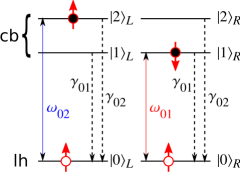
Figure 7: Reduced model for the numerical simulation of CHSH inequality violation in the presence of electronic decoherence. The dashed arrows represent non-radiative electronic decoherence.

Appendix E Entanglement in the presence of electronic decoherence

In the main text we have assumed that the photon emission process takes place on a time scale short compared to the coherence time $T_{2}$ of the QDs. Here, we investigate numerically the effect of electronic decoherence on the CHSH inequality violation of the intra-cavity photon state for a perfect cavity with $\kappa=0$. To this end we consider the reduced QD model consisting of two three-level “atoms”, each resonantly coupled to two cavity modes as depicted in Fig. 7.

We shall consider electronic relaxation determined by the non-radiative relaxation rates $\gamma_{01}$ and $\gamma_{02}$ for transitions from states $\left|{2}\right\rangle$ and $\left|{1}\right\rangle$ to the state $\left|{0}\right\rangle$ as well as electronic dephasing with rates $\gamma_{01}^{\varphi}$ and $\gamma_{02}^{\varphi}$ due to fluctuations of the corresponding transition energies. This corresponds to an effective coherence time for the double dot of $T_{2}\approx 1/(\gamma_{01}/2+\gamma_{02}/2+\gamma_{01}^{\varphi}+\gamma_{02}^{\varphi})$. As before, the Hamiltonian of both QD-cavity systems decouples into a sum as $H=H_{L}+H_{R}$ with (we set $\hbar=1$)

$$H_{\alpha} =\omega_{01}\left(\left|{1}\right\rangle\left<{1}\right|+a_{\alpha}^{\dagger}a_{\alpha}\right)+\omega_{02}\left(\left|{2}\right\rangle\left<{2}\right|_{\alpha}+b_{\alpha}^{\dagger}b_{\alpha}\right)$$

$$+g\left(\left|{0}\right\rangle\left<{1}\right|_{\alpha}a_{\alpha}^{\dagger}+\left|{0}\right\rangle\left<{2}\right|_{\alpha}b_{\alpha}^{\dagger}+{\rm h.c.}\right),\quad\alpha\in\{L,R\}.$$ (53)

Note that, in order to most clearly distinguish the effect of decoherence from other effects, we choose equal coupling strength $g$ for both transitions. The evolution of the state of the system $\rho$, is described within the Born-Markov approximation by the zero-temperature Lindblad master equation

$$\dot{\rho} =-i[H,\rho]+\sum_{\alpha=L,R}\left(\gamma_{01}\mathcal{D}[\sigma_{01}^{\alpha,-}]+\gamma_{02}\mathcal{D}[\sigma_{02}^{\alpha,-}]\right)\rho$$

$$+\sum_{\alpha=L,R}\left(\gamma_{01}^{\varphi}\mathcal{D}[\sigma_{01}^{\alpha,z}]+\gamma_{02}^{\varphi}\mathcal{D}[\sigma_{02}^{\alpha,z}]\right)\rho,$$ (54)

with $\mathcal{D}[O]\rho=\left(2O\rho O^{\dagger}-O^{\dagger}O\rho-\rho O^{\dagger}O\right)/2$, $\sigma_{ij}^{\alpha,-}=\left|{i}\right\rangle\left<{j}\right|_{\alpha}$ and $\sigma_{ij}^{\alpha,z}=\left|{j}\right\rangle\left<{j}\right|_{\alpha}-\left|{i}\right\rangle\left<{i}\right|_{\alpha}$. The photonic state $\rho_{\rm ph}={\rm tr}_{\rm el}\left[\rho\right]$, is obtained by tracing $\rho$ over the electronic degrees of freedom. Fig. 8 shows the CHSH correlation of Eq. (23) as a function of the relative angle $\theta$ between left and right observers, for $T_{2}g\approx 26.7$. While decoherence clearly weakens the CHSH correlation, this simulation essentially demonstrates that as long as the coupling strength $g$ is large compared with the decoherence rate $T_{2}^{-1}$ of the QD, the CHSH inequality can be violated.

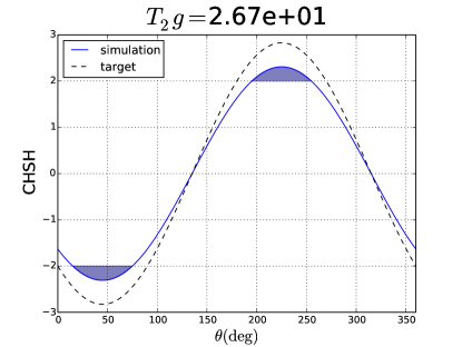
Figure 8: Violation of the CHSH inequality with the cavity photons in the presence of electronic decoherence. The shaded areas indicate regions where the CHSH inequality is violated.

Appendix F Effect of cavity cross-talk

In this appendix we investigate quantitatively to what extent cavity cross-talk affects our entanglement transfer scheme. To this end we perform a numerical simulation of the coherent system including a polarization conserving cavity-cavity coupling term of the form $g_{\rm ph}(a_{L}^{\dagger}a_{R}+b_{L}^{\dagger}b_{R}+{\rm h.c.})$. We use the notation of Appendix E.

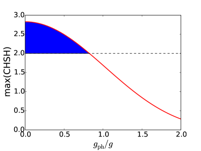
Figure 9: Maximal violation of the CHSH inequality after half a Rabi period in the presence of inter-cavity coupling with strength $g_{\rm ph}$. When the inter-cavity coupling is weaker than roughly the electron-photon coupling in each cavity, the CHSH inequality is violated (shaded area).

Fig. 9 shows the maximal Bell inequality violation achievable after half a (bare) Rabi period $\sim 1/g$. We see that while the correlation signal is clearly reduced by a finite inter-cavity coupling, it still surpasses the threshold of $2.0$ demonstrating entanglement, roughly as long as $g_{\rm ph}<g$. Furthermore, in the experimentally relevant case where the photons are coupled out of the cavities, the population of the cavity modes remains small at all times and is of order $(g/\kappa)^{2}\ll 1$ (see Appendix. D and panel (c) of Fig. 5). Hence the effective cavity-cavity coupling rate is reduced compared with the coherent case.

Appendix G Typical values of the parameters

In this appendix, we estimate the typical range of values for various parameters used in our theory. A typical value of the coupling strength between the quantum dot and the cavity field is $g\approx 20$ GHz [Yoshie et al., 2004]. Choosing a cavity decay rate of $\kappa\approx 100$ GHz, leads to an induced bandwidth of $g^{2}/\kappa\approx 4$ GHz for the conduction band levels. The Zeeman splitting for a magnetic field strength of 10 mT is $\sim 0.1$ GHz. Thus for these parameters by using a magnetic field which is weaker than 10 mT, Bell’s inequality can be violated. A typical intrinsic coherence time of the self-assembled quantum dots is $T_{2}\sim 0.1$ $\mu$s ($1/T_{2}\sim 0.01$ GHz) [Kloeffel and Loss, 2013]. A typical value of Cooper pair splitting rate is $\Gamma_{c}\approx 2$ GHz [Herrmann et al., 2010]. Thus the various conditions ($g^{2}/\kappa\gg\Delta_{Z}^{\textrm{(cb)}}$, $g/\kappa\ll 1$, $g^{2}/\kappa\gg 1/T_{2}$, and $\Gamma_{c}\gg 1/T_{2}$) essential for demonstrating entanglement in our scheme, can be satisfied with current technology.

References

- Schrödinger (1935) E. Schrödinger, Math. Proc. Cambridge 31, 555 (1935).
- Bouwmeester et al. (1997) D. Bouwmeester, J.-W. Pan, K. Mattle, M. Eibl, H. Weinfurter, and A. Zeilinger, Nature 390, 575 (1997).
- Jozsa and Linden (2003) R. Jozsa and N. Linden, Proc. R. Soc. A 459, 2011 (2003).
- Jennewein et al. (2000) T. Jennewein, C. Simon, G. Weihs, H. Weinfurter, and A. Zeilinger, Phys. Rev. Lett. 84, 4729 (2000).
- Giovannetti et al. (2011) V. Giovannetti, S. Lloyd, and L. Maccone, Nat. Photonics 5, 222 (2011).
- Bell (1964) J. S. Bell, Physics 1, 195 (1964).
- Aspect et al. (1982) A. Aspect, J. Dalibard, and G. Roger, Phys. Rev. Lett. 49, 1804 (1982).
- Einstein et al. (1935) A. Einstein, B. Podolsky, and N. Rosen, Phys. Rev. 47, 777 (1935).
- Bennett and DiVincenzo (2000) C. H. Bennett and D. P. DiVincenzo, Nature 404, 247 (2000).
- Choi et al. (2000) M.-S. Choi, C. Bruder, and D. Loss, Phys. Rev. B 62, 13569 (2000).
- Recher et al. (2001) P. Recher, E. V. Sukhorukov, and D. Loss, Phys. Rev. B 63, 165314 (2001).
- Lesovik et al. (2001) G. B. Lesovik, T. Martin, and G. Blatter, Eur. Phys. J. B 24, 287 (2001).
- Hofstetter et al. (2009) L. Hofstetter, S. Csonka, J. Nygard, and C. Schönenberger, Nature 461, 960 (2009).
- Herrmann et al. (2010) L. G. Herrmann, F. Portier, P. Roche, A. Levy Yeyati, T. Kontos, and C. Strunk, Phys. Rev. Lett. 104, 026801 (2010).
- Das et al. (2012) A. Das, Y. Ronen, M. Heiblum, D. Mahalu, A. V. Kretinin, and H. Shtrikman, Nat. Comm. 3, 1165 (2012).
- Tiwari et al. (2012) R. P. Tiwari, W. Belzig, M. Sigrist, and C. Bruder, Phys. Rev. B 89, 184512 (2014).
- Walter et al. (2012) S. Walter, J. C. Budich, J. Elsert, and B. Trauzettel, Phys. Rev. B 88, 035441 (2013).
- Cottet et al. (2012) A. Cottet, T. Kontos, and A. Levy Yeyati, Phys. Rev. Lett. 108, 166803 (2012).
- Kawabata (2001) S. Kawabata, J. Phys. Soc. Jpn. 70, 1210 (2001).
- Braunecker et al. (2013) B. Braunecker, P. Burset, and A. Levy Yeyati, Phys. Rev. Lett. 111, 136806 (2013).
- Cottet (2014) A. Cottet (2014), arXiv:1406.4666 [cond-mat.mes-hall].
- Chtchelkatchev et al. (2002) N. M. Chtchelkatchev, G. Blatter, G. B. Lesovik, and T. Martin, Phys. Rev. B 66, 161320 (2002).
- Scherübl et al. (2014) Z. Scherübl, A. Pályi, and S. Csonka, Phys. Rev. B 89, 205439 (2014).
- Burkard et al. (2000) G. Burkard, D. Loss, and E. V. Sukhorukov, Phys. Rev. B 61, R16303 (2000).
- Veronica Cerletti, Oliver Gywat, and Daniel Loss (2005) V. Cerletti, O. Gywat, and D. Loss, Phys. Rev. B 72, 115316 (2005).
- Jan Budich and Björn Trauzettel (2010) J. Budich, and B. Trauzettel, Nanotechnology 21, 274001 (2010).
- (27) In particular, in order to disentangle the electronic from the photonic degrees of freedom, the photon emitters need to be prepared in a quantum superposition state.
- Brossard et all. (2013) F. S. F. Brossard, B. P. L. Reid, C. C. S. Chan, X. L. Xu, J. P. Griffiths, D. A. Williams, R. Murray, R. A. Taylor, Opt. Express 21, 16934–16945 (2013).
- Schroer (2014) A. Schroer, and P. Recher, (2014), arXiv:1412.8619 [cond-mat.supr-con].
- Kim et al. (2004) S.-H. Kim, S.-K. Kim, and Y.-H Lee, Phys. Rev. B 73, 235117 (2006).
- Tran et al. (2009) N.-V.-Q. Tran, S. Combrié, and A. De Rossi, Phys. Rev. B 79, 041101 (2009).
- Portalupi et al. (2010) S. L. Portalupi, M. Galli, C. Reardon, T. F. Krauss, L. O’Faolain, L. C. Andreani, and D. Gerace, Optics Express 18, 16064 (2010).
- Yoshie et al. (2004) T. Yoshie, A. Scherer, J. Hendrickson, G. Khitrova, H. M. Gibbs, G. Rupper, C. Ell, O. B. Shchekin, and D. G. Deppe, Nature 432, 200 (2004).
- Majumdar et al. (2013) A. Majumdar, P. Kaer, M. Bajcsy, E. D. Kim, K. G. Lagoudakis, A. Rundquist, and J. Vučković, Phys. Rev. Lett. 111, 027402 (2013).
- Sweeney et al. (2014) T. M. Sweeney, S. G. Carter, A. S. Bracker, M. Kim, C. S. Kim, L. Yang, P. M. Vora, P. G. Brereton, E. R. Cleveland, and D. Gammon, Nat. Photonics 8, 442 (2014).
- Gywat et al. (2010) O. Gywat, H. Krenner, and J. Berezovsky, Spins in Optically Active Quantum Dots (Wiley-VCH, 2010).
- Clauser et al. (1969) J. F. Clauser, M. A. Horne, A. Shimony, and R. A. Holt, Phys. Rev. Lett. 23, 880 (1969).
- Weisskopf and Wigner (1930) V. Weisskopf and E. Wigner, Z. Phys. 63, 54 (1930).
- Jaynes and Cummings (1963) E. Jaynes and F. Cummings, Proc. IEEE 51, 89 (1963).
- Vidal and Werner (2002) G. Vidal and R. F. Werner, Phys. Rev. A 65, 032314 (2002).
- Kloeffel and Loss (2013) C. Kloeffel and D. Loss, Annu. Rev. Condens. Matter Phys. 4, 51 (2013).