Discrete solitons and vortices on two-dimensional lattices of $\mathcal{PT}$-symmetric couplers

Abstract

We introduce a 2D network built of $\mathcal{PT}$-symmetric dimers with on-site cubic nonlinearity, the gain and loss elements of the dimers being linked by parallel square-shaped lattices. The system may be realized as a set of $\mathcal{PT}$-symmetric dual-core waveguides embedded into a photonic crystal. The system supports $\mathcal{PT}$-symmetric and antisymmetric fundamental solitons (FSs) and on-site-centered solitary vortices (OnVs). Stability of these discrete solitons is the central topic of the consideration. Their stability regions in the underlying parameter space are identified through the computation of stability eigenvalues, and verified by direct simulations. Symmetric FSs represent the system’s ground state, being stable at lowest values of the power, while anti-symmetric FSs and OnVs are stable at higher powers. Symmetric OnVs, which are also stable at lower powers, are remarkably robust modes: on the contrary to other $\mathcal{PT}$-symmetric states, unstable OnVs do not blow up, but spontaneously rebuild themselves into stable FSs.
OCIS codes: (190.6135) Spatial solitons; (190.3100) Instabilities and chaos; (050.5298) Pho- tonic crystals; (130.2790) Guided waves.

I Introduction

Dynamics of light fields in dissipative media keeps drawing much interest in nonlinear optics review0 ; review . A special kind of such systems with exactly balanced spatially separated gain and loss realize the general concept of the parity-time ($\mathcal{PT}$)-symmetry Bender1 ; Bender2 . $\mathcal{PT}$-symmetric systems are represented by Hamiltonians containing a complex potential, $V(\mathbf{r})$, which is subject to the symmetry constraint, $V(\mathbf{r})=V^{\ast}(-\mathbf{r})$. In optics this condition can be realized by guiding light through a medium with a complex refractive index satisfying condition $n(\mathbf{r})=n^{\ast}(-\mathbf{r})$ Muga ; Makris ; Klaiman ; Guo ; Longhi1 ; Longhi2 ; Makris2 ; coupled-mode , hence its real and imaginary part, the latter one representing the combination of spatially distributed gain and loss, must be, respectively, even and odd functions of spatial coordinates.

Unlike generic dissipative systems, in which the balance between gain and loss selects parameters of isolated stable modes (attractors), $\mathcal{PT}$-symmetric settings support continuous families of modes, sharing this property with conservative media, which was a motivation for many experimental Regensburger ; exper and theoretical studies, including the consideration of a great diversity of nonlinear $\mathcal{PT}$-symmetric systems Musslimani ; Zhuxing ; Yaro ; Lihuagang ; Radik ; oligo ; Miro ; Barash ; Nixon ; Abd ; Alexeeva ; Uwe ; birefr ; Thawatchai ; Flach ; Burlak ; Hadi ; Romania ; restoration ; Yang ; SYS ; unbreakable . In the latter case, solitons are a major subject of the studies.

An important variety of $\mathcal{PT}$-symmetric systems in optics are discrete ones. The simplest among them, which was actually the first $\mathcal{PT}$-symmetric system created experimentally Moti , is realized as a pair of linearly coupled waveguides carrying gain and loss with equal strengths (a dimer oligo ; Miro ; Uwe ; birefr ; Flach ; Hadi ). An extension to various more complex discrete systems is provided by arrays of linearly coupled dimers Dmitriev ; Suchkov ; Suchkov2 ; Suchkov3 ; Zezyulin ; Konotop ; Leykam ; Tsironis ; Peli ; Xiangyu ; AubryAndre . In particular, robust one-dimensional (1D) discrete solitons Suchkov and scattering states Suchkov3 are supported by a chain of dimers with the cubic nonlinearity, in which active (gain-carrying) and passive (lossy) elements are coupled horizontally, while at each site the active and passive poles are coupled vertically. Accordingly, the chain is described by a system of linearly coupled discrete nonlinear Schrödinger (DNLS) equations with equal strengths of linear gain and loss in the two components. Stability, mobility and interactions between fundamental discrete solitons in this system were studied by means of numerical methods and analytical approximations.

There are fewer publications which reported $\mathcal{PT}$-symmetric solitons in 2D settings Nixon ; Burlak ; SYS . The objective of the present work is to introduce a 2D network of horizontally coupled nonlinear dimers, which is a generalization of the 1D system from Suchkov , and can also be realized in optics, using a photonic-crystal matrix into which nonlinear dual-core waveguides with the balanced gain and loss are embedded (see Fig. 1 below). We construct families of fundamental and vortical two-component discrete solitons in this 2D system and analyze their stability.

The paper is structured as follows. The model is introduced in Section 2. Fundamental and vortex solitons are produced in Sections 3 and 4, respectively. The paper is concluded by Section 5.

II Model

The network model, outlined above as the 2D extension of the chain of dimers introduced in Suchkov , is based on a system of two linearly coupled normalized DNLS equations for amplitudes $\psi_{m,n}(z)$ and $\varphi_{m,n}(z)$ of the electromagnetic field propagating in the active and passive cores of dual-core waveguides (that represent the $\mathcal{PT}$-symmetric dimers), which, as schematically shown in Fig. 1, are embedded into a quasi-2D photonic crystal, built of thin plates connecting the active and passive cores into respective sub-networks:

$$i{\frac{d}{dz}}\psi_{m,n}=-{\frac{C}{2}}(\psi_{m,n+1}+\psi_{m,n-1}+\psi_{m-1,n}+\psi_{m+1,n}-4\psi_{m,n})-|\psi_{m,n}|^{2}\psi_{m,n}-\varphi_{m,n}+i\gamma\psi_{m,n},$$

$$i{\frac{d}{dz}}\varphi_{m,n}=-{\frac{C}{2}}(\varphi_{m,n+1}+\varphi_{m,n-1}+\varphi_{m-1,n}+\varphi_{m+1,n}-4\varphi_{m,n})-|\varphi_{m,n}|^{2}\varphi_{m,n}-\psi_{m,n}-i\gamma\varphi_{m,n}.$$ (1)

Here $\left(m,n\right)$ are discrete coordinates in the transverse plane, $z$ is the propagation distance, the coefficient of the coupling between the active and passive cores is scaled to be $1$, $\gamma>0$ is the gain-loss coefficient, and $C$ is coupling constant in the networks. Localized states produced by Eq. (1) are characterized by the total power,

$$P=\sum{}_{m,n}\left(|\psi_{m,n}|^{2}+|\varphi_{m,n}|^{2}\right).$$ (2)

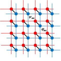
Figure 1: The transverse cross-section of the waveguiding system built as a juxtaposition of networks of active (red) and passive (blue) elements, which are coupled into $\mathcal{PT}$-symmetric dimers (the couplings are designated by short diagonal segments). The elements are connected into the networks by thin plates forming the double photonic crystal. The propagation axis ($z$) is directed perpendicular to the plane of the drawing.

To estimate physical parameters of the setting, we assume that it is built of AlGaAs (the nonlinear coefficient of this material is $n_{2}\simeq 1.5\times 10^{-13}$ cm²/W Aitchison ), with core area $4$ $\mathrm{\mu}$m² of the lattice site, and refractive indices of the core and thin plates $3.263$ and $3.256$, respectively (the corresponding refractive-index difference can be produced by varying the share of aluminium in the composition of those parts). The standard coupled-mode theory Yariv ; Zhijie shows that, if we fix the distance between the adjacent active and passive lattice sites as $4$ $\mathrm{\mu}$m, the coupling coefficient between them is $3.6$ mm^-1. Because we scale this coefficient to be $1$ in Eq. (1), we can estimate the accordingly normalized values of the coupling and gain-loss coefficients, $C$ and $\gamma$, and the unit of the total power, $P_{0}=0.55$ kW. For example, the lattice spacing$\ 8$ $\mathrm{\mu}$m and the physical value of the gain-loss coefficient, $1.8$ mm ^-1, imply $C=0.3$ and $\gamma=0.5$. These values are realistic for the experimental realization, and, on the other hand, their normalized values give rise to nontrivial results, as shown below.

Stationary modes with real propagation constant $k$ are looked for as solutions to Eq. (1) as usual, $\left\{\psi_{m,n}(z),\varphi_{m,n}(z)\right\}=e^{ikz}\left\{u_{m,n},v_{m,n}\right\}$, where stationary amplitudes obey equations in the form of

$$\left(k+i\gamma\right)u_{m,n} = {\frac{C}{2}}(u_{m,n+1}+u_{m,n-1}+u_{m-1,n}+u_{m+1,n}-4u_{m,n})+|u_{m,n}|^{2}u_{m,n}+v_{m,n},$$

$$\left(k-i\gamma\right)v_{m,n} = {\frac{C}{2}}(v_{m,n+1}+v_{m,n-1}+v_{m-1,n}+v_{m+1,n}-4v_{m,n})+|v_{m,n}|^{2}v_{m,n}+u_{m,n}.$$ (3)

Because our study is focused on localized modes, we apply zero boundary conditions at infinity (in fact, at edges of the numerical domain).

In the numerical simulations, it is convenient to combine $u_{m,n}$ and $v_{m,n}$ into a single “long” vector, $U$, of length $2N^{2}$, where $N\times N$ is the size of the numerical domain. Thus, Eq. (3) is rewritten in the vectorial form:

$$\hat{L}U-\mathrm{\mathbf{diag}}(|U|^{2})U=-\left(k+i\hat{\Gamma}\right)U,$$ (4)

where $\mathrm{\mathbf{diag}}(|U|^{2})$ means a diagonal matrix with the respective elements, the other matrices being $\hat{L}=\left(\begin{array}[]{cc}\mathbf{D}&-\mathbf{I}\\ -\mathbf{I}&\mathbf{D}\end{array}\right)$ and $\hat{\Gamma}=\gamma\left(\begin{array}[]{cc}\mathbf{I}&0\\ 0&-\mathbf{I}\end{array}\right)$, where $\mathbf{I}$ and $\mathbf{D}$ are, respectively, the $N^{2}\times N^{2}$ unit and linear-coupling matrices, the latter one built of elements $D_{j,j^{\prime}}=-\left(C/2\right)(\delta_{j,j^{\prime}-N}+\delta_{j,j^{\prime}-1}+\delta_{j,j^{\prime}+1}+\delta_{j,j^{\prime}+N}-4\delta_{j,j^{\prime}})$. The stability of the stationary modes is investigated in a numerical form, computing eigenvalues for small perturbations and verifying the results by direct simulations. Linearized equations for perturbation eigenmodes are produced by writing the perturbed solution, in terms of the “long vector”, $U$, as $\left\{\psi_{m,n}(z),\varphi_{m,n}(z)\right\}=e^{ikz}(U+\alpha e^{-i\lambda z}+\beta^{\ast}e^{i\lambda^{\ast}z})$, where $\alpha$ and $\beta$ are the respective vectors combining amplitudes of the eigenmodes, and $\ast$ stands for the complex conjugation:

$$\left(\begin{array}[]{cc}\hat{L}+k-2\mathrm{\mathbf{diag}}(|U|^{2})+i\hat{\Gamma}&-\mathrm{\mathbf{diag}}(U^{2})\\ \mathrm{\mathbf{diag}}(U^{\ast 2})&-\hat{L}-k+2\mathrm{\mathbf{diag}}(|U|^{2})+i\hat{\Gamma}\end{array}\right)\left(\begin{array}[]{c}\alpha\\ \beta\end{array}\right)=\lambda\left(\begin{array}[]{c}\alpha\\ \beta\end{array}\right).$$ (5)

The underlying solution, $U$, is stable if all eigenvalues $\lambda$ are real.

III Fundamental solitons

III.1 Symmetric modes

As suggested by the analysis of the $\mathcal{PT}$-symmetric coupler Radik ; Barash , the parity-time symmetry of Eqs. (1) remains unbroken at $\gamma<1$, in which case the system of two coupled equations (3) can be reduced to a single one,

$$\left(-k\pm\sqrt{1-\gamma^{2}}\right)u_{m,n}+{\frac{C}{2}}\left(u_{m,n+1}+u_{m,n-1}+u_{m-1,n}+u_{m+1,n}-4u_{m,n}\right)+|u_{m,n}|^{2}u_{m,n}=0,$$ (6)

by substitution

$$v_{m,n}=e^{i\chi_{\pm}}u_{m,n},~{}\chi_{+}=\arcsin\gamma,~{}~{}\chi_{-}=\pi-\arcsin\gamma,$$ (7)

with $\pm$ in Eq. (6) corresponding to $\chi_{\pm}$ in Eq. (7). Because in the limit of $\gamma=0$ relation (7) with $\chi_{+}$ and $\chi_{-}$ represents, respectively, symmetric and antisymmetric states in the two-component conservative system, these solutions may be naturally named $\mathcal{PT}$-symmetric and antisymmetric ones Radik .

Discrete 2D fundamental solitons (FSs) in the conservative version of Eqs. (1) and (3) with $\gamma=0$ were previously studied in the context of the spontaneous formation of asymmetric solitons, with $u_{m,n}\neq v_{m,n}$, from the symmetric ones Herring . The transition to asymmetric solitons is not relevant for $\mathcal{PT}$-symmetric systems, where the spontaneous symmetry breaking causes blow-up, rather than emergence of asymmetric modes Radik ; Barash ) (recently, it was demonstrated that asymmetric solitons may exist in a specially designed 1D $\mathcal{PT}$-symmetric model Yang ). However, the instability may lead, instead of the blow-up, to transformation into a stable soliton of another type, if different solitons species coexist in the system. In particular, it is demonstrated below that unstable $\mathcal{PT}$-symmetric solitary vortices do not blow up, but rather rebuild themselves into stable symmetric FSs.

Equation (6) is the usual stationary form of the 2D DNLS equation, which gives rise to discrete FSs Panos and solitary vortices Malomed whose total power (2) grows with the increase of the effective propagation constant,

$$k_{\mathrm{eff}}=k\mp\sqrt{1-\gamma^{2}},$$ (8)

so that these modes satisfy the Vakhitov-Kolokolov criterion VK ; Berge' , $dP/dk>0$, which is a necessary, but not sufficient, condition for their stability. Therefore, for given $k$, term $\mp\sqrt{1-\gamma^{2}}$ in Eq. (8) makes the total power of the $\mathcal{PT}$-symmetric FS smaller than that of its antisymmetric counterpart. The latter fact, in turn, implies that the symmetric FS may represent the system’s ground state (it is demonstrated below that this conjecture is true), and it should be more relevant to the experiment, as the creation of the mode with a smaller power is, obviously, easier.

Stationary solutions for symmetric FSs were produced, first, by means of the imaginary-time-propagation method (ITM) gs , applied to Eq. (1). For these computations, the set of control parameters includes the gain-loss and coupling strengths, $\left(\gamma,C\right)$, and the total power of the soliton, $P$. It was checked that precisely the same family of symmetric solutions is generated by the Newton’s method applied to stationary equations (4). The fact that these solutions are produced by the ITM method strongly suggests that they indeed represent the system’s ground state Tosi . It is also relevant to stress that Eq. (4) produces exactly the same solutions as the reduced equation (6), although reduction (7) was not applied to Eq. (4). A typical example of a stable $\mathcal{PT}$-symmetric FS is displayed in Fig. 2.

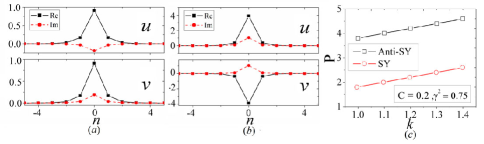
Figure 2: (a) The cross-section, along $m=0$, of a typical $\mathcal{PT}$-symmetric fundamental soliton produced by Eq. (1), with $(C,\gamma)=(0.3,0.4)$, and total power $P=2$. Its real and imaginary parts precisely obey Eq. (7) with $\chi=\chi_{+}$. Both the computation of stability eigenvalues and direct simulations demonstrate that this soliton is stable. (b) The cross-section (along $m=0$) of a typical stable $\mathcal{PT}$-antisymmetric fundamental soliton, which is also stable, produced by stationary equations (1) for $(C,\gamma)=(3,0.5)$, and $k=10$. The total power of this soliton is $P=33.8$. (c) $P(k)$ dependences for the symmetric (“SY”) and antisymmetric (“Anti-SY”) fundamental solitons, with $C=0.2$ and $\gamma=\sqrt{3}/2$. The fitting result for them is $P(k)=4C+2k\mp 1$, which is consistent with Eq. (11).

For $\gamma=0$, the results corroborate well-known properties of the 2D FSs in the DNLS equation Panos . In particular, symmetric on-site-centered FSs (their off-site-centered counterparts are completely unstable, as usual Panos , and are not considered here) exist above a power threshold,

$$P>P_{\mathrm{th}}^{(1)}=\mathrm{const}\cdot C,~{}\mathrm{const}\approx 5.7.$$ (9)

Because stationary equations (3) for $\mathcal{PT}$-symmetric modes reduce to the single equation (6), it is obvious that $P_{\mathrm{th}}^{(1)}$ does not depend on $\gamma$. Further, if the $P(k)$ dependence for the FS in the single-component DNLS equation with $\gamma=0$ is $P_{1}(k)$, which is well known in the numerical form Panos , then an exact result for the two-component $\mathcal{PT}$-symmetric and antisymmetric FSs, following from Eq. (6), is

$$P=2P_{1}\left(k\mp\sqrt{1-\gamma^{2}}\right).$$ (10)

Numerical solutions for both types of the solitons completely agree with Eq. (10) (not shown here in detail). In fact, for both the $\mathcal{PT}$-symmetric and antisymmetric FSs the $P(k)$ dependence can be rather accurately fitted to an empiric relation

$$P_{\mathrm{FS}}(k,\gamma)\approx 2\left(2C+k\mp\sqrt{1-\gamma^{2}}\right).$$ (11)

Figure 2(c) displays the typical examples of such numerical fitting. In particular, the known results for the stable 2D FS in the usual DNLS equation, corresponding to $\gamma=0$ Panos , are indeed close to the approximate linear dependence obtained for this case from Eq. (11), $P_{1}(k)\approx 2C+k$.

An essential finding is that the symmetric FS becomes unstable above a higher threshold value of the total power, $P=P_{\mathrm{th}}^{(2)}$. This stability boundary may be understood as the one at which the symmetric soliton is destabilized by the spontaneous symmetry breaking, modified by the presence of $\gamma>0$ in comparison with the similar effect in the conservative system with $\gamma=0$ Herring . Because asymmetric solitons cannot exist in the system with the balanced gain and loss, this symmetry breaking always leads to blow-up of the FS in the active component [$\psi_{m,n}$ in Eq. (1)]. The blow-up is quite similar to that shown below in Fig. 7(b) for an antisymmetric vortex.

The most essential results of the numerical analysis of the $\mathcal{PT}$-symmetric FSs are summarized in Fig. 3, in the form of stability diagrams in parameter planes $\left(\gamma,C\right)$, $\left(\gamma,P\right)$, and $\left(C,P\right)$. The horizontal and diagonal cutoffs in the $\left(\gamma,C\right)$, $\left(\gamma,P\right)$ and $\left(C,P\right)$ planes exactly represent the threshold power, as given by Eq. (9). A natural trend is shrinkage of the stability area with the increase of $\gamma$, and its full disappearance close to $\gamma=1$. It is natural as well that the stability area expands with the increase of $C$ at fixed $P$, because the large coupling constant makes the modes, effectively, “less nonlinear”, for the given total power, and this, in turn, suppresses the trend to the nonlinearity-driven spontaneous symmetry breaking which destabilizes the soliton.

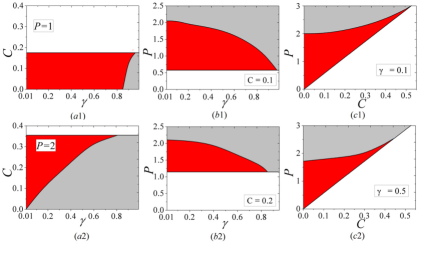
Figure 3: Here and in similar figures below, red and gray colors represent, respectively, stability and instability areas – here, for $\mathcal{PT}$-symmetric fundamental solitons – as found from the computation of the stability eigenvalues [see Eq. (5)], and verified by direct simulations. In white areas, soliton solutions cannot be found. The red-white and red-gray boundaries correspond, severally, to threshold values $P_{\mathrm{th}}^{(1)}$ and $P_{\mathrm{th}}^{(2)}$ (see the text).

III.2 Antisymmetric solitons

It has been found that the system supports stable and unstable antisymmetric FSs too [see a typical examples of a stable one in Fig. 2(b)]. The antisymmetric FSs cannot be produced by the ITM, which suggests that, as argued above, they do not represent the system’s ground state. Nevertheless, they have been generated by the Newton’s method applied to Eq. (4). For this reason, the propagation constant, $k$, rather than the total power, $P$, plays the role of the control parameter for the antisymmetric solitons. Their stability was identified through a numerical solution of Eq. (5), and verified by means of direct simulations of Eq. (1). Results of the stability analysis are collected in Fig. 4, in which panels (a-c) display the stability area in the $\left(k,C\right)$ and $\left(\gamma,C\right)$ panels. In addition, the stability area is mapped into the $\left(C,P\right)$ plane in plot 4(d), using the $P(k)$ dependence [see Eq. (11)]. In the latter panel, the boundary of the white non-existence area is given by Eq. (9), i.e., it is exactly the same as in Fig. 3(c1) and 3(c2), once the existence of both symmetric and antisymmetric FSs is determined by the same equation, Eq. (6).

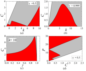
Figure 4: (a,b) The stability area (red) of the antisymmetric fundamental solitons for (a) $\gamma=0.5$ and (b) $\gamma=0.999$. (c) The stability area in the $(\gamma,C)$ plane for $k=10$. (d) The stability diagram for $\gamma=0.5$ in the $(C,P)$ plane.

We have found that, at $\gamma<0.95$, the stability area shown in panel 4(d) tends to extend to $P\rightarrow\infty$ [or, in other words, to $k\rightarrow\infty$ in panel 4(a)], up to the accuracy limits of the numerical calculations. This conclusion is in drastic contrast with the situation shown for the symmetric FSs in Fig. 3, where the stability is always bounded from above, in terms of $P$. The explanation for the stability of the antisymmetric solitons at large $P$ is straightforward: unlike their symmetric counterparts, they do not undergo the destabilization via the symmetry breaking at large $P$. However, at $\gamma>0.95$, the stability area becomes finite in terms of $k$, see Fig. 4(c) for $\gamma=0.999$. Although the area is not vanishingly small at $\gamma$ so close to $1$, it exactly collapses to nil at $\gamma=1$, as it should, as the $\mathcal{PT}$ symmetry gets completely broken at this point.

A general conclusion about the antisymmetric FSs (which pertains equally well to antisymmetric vortex solitons, see below) is that, although they tend to be stable at large values of the power, where their symmetric counterparts are unstable, they are less suitable for the experimental realization just because they demand large powers for the stability, while the symmetric FS, which represents the ground state of the system, may be stable at lower levels of the power.

IV Vortex soliton

To the best of our knowledge, the symmetry breaking of discrete vortex solitons in 2D two-component linearly-coupled lattices was not investigated even in the conservative model, with $\gamma=0$. We have found symmetric, antisymmetric, and asymmetric solitary vortices, and the symmetry-breaking transition, in the model based on Eqs. (1) and (3) with $\gamma=0$. These findings will be reported elsewhere, while here we focus on $\mathcal{PT}$-symmetric and antisymmetric vortices in the system with $\gamma>0$ (in fact, it is shown below that, for symmetric vortices, the stability area only weakly changes with the variation of $\gamma$, hence the present results give an idea of the stability of symmetric vortices in the conservative system too). Because the ITM cannot converge to the definitely non-ground-state vortical modes, the solutions were found by means of the Newtons’s method applied to Eq. (4), hence the control parameter of the solution families is the propagation constant, $k$, rather than total power $P$.

It is well known that two types of vortices are possible in discrete systems, viz., on- and off-site-centered ones Panos (alias “rhombuses” and “squares”). Both can be produced by the Newton’s method applied to Eq. (3), starting from the following inputs:

$$\left\{u_{m,n},v_{m,n}\right\}_{\mathrm{on}}=\left\{\begin{array}[]{c}\left\{U,V\right\}~{}~{}\mathrm{at}~{}~{}\left(m,n\right)=\left(0,1\right),\\ i\left\{U,V\right\}~{}~{}\mathrm{at}~{}~{}\left(m,n\right)=\left(1,0\right),\\ -\left\{U,V\right\}~{}~{}\mathrm{at}~{}~{}\left(m,n\right)=\left(-1,0\right),\\ -i\left\{U,V\right\}~{}~{}\mathrm{at}~{}~{}\left(m,n\right)=\left(0,-1\right),\\ 0,~{}\mathrm{at~{}all~{}others}~{}~{}\left(m,n\right),{}{}{}\end{array}\right.$$ (12)

$$\left\{u_{m,n},v_{m,n}\right\}_{\mathrm{off}}=\left\{\begin{array}[]{c}\left\{U,V\right\}~{}~{}\mathrm{at}~{}~{}\left(m,n\right)=\left(0,0\right),\\ i\left\{U,V\right\}~{}~{}\mathrm{at}~{}~{}\left(m,n\right)=\left(1,0\right),\\ -\left\{U,V\right\}~{}~{}\mathrm{at}~{}~{}\left(m,n\right)=\left(1,1\right),\\ -i\left\{U,V\right\}~{}~{}\mathrm{at}~{}~{}\left(m,n\right)=\left(0,1\right),\\ 0,~{}\mathrm{at~{}all~{}others}~{}~{}\left(m,n\right),{}\end{array}\right.$$ (13)

where $U$ and $V$ are real constants.

In agreement with the known result for the usual 2D DNLS equation with $\gamma=0$ Malomed , we have found that the off-site vortices are unstable at practically all values $C>0$ (they may be stable at extremely small $C$), therefore in what follows below we consider only the modes of the on-site types.

As well as in the case of FSs, stationary solutions for on-site-centered vortices (OnVs) are subject to reduction (7), which leads to the single equation (6), hence the OnV may also be classified into $\mathcal{PT}$ symmetric or antisymmetric varieties. Examples of stable symmetric and antisymmetric ones are displayed in Figs. 5 and 6.

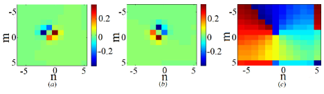
Figure 5: Real (a) and imaginary (b) parts, and the phase structure (c), of field $u_{m,n}$ of a typical stable $\mathcal{PT}$-symmetric vortex soliton, for $(C,\gamma)=(0.06,0.4)$ and $k=1$ ($P=1.65$).

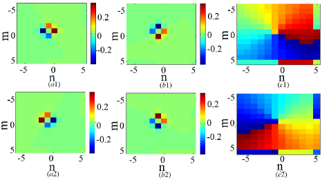
Figure 6: The same as in Fig. 5, but for a stable $\mathcal{PT}$-antisymmetric vortex, for $(C,\gamma)=(2,0.85)$ and $k=8$ ($P=100.3$). In this figure, both components are displayed, to stress that relation (7) for the antisymmetric vortex, with $\chi=\chi_{-}$, gives rise to rotation of the phase pattern by angle $\pi-\arcsin\left(0.85\right)\approx 0.7\pi$.

A unique dynamical property of the symmetric OnVs is that, when they are unstable, they do not blow up, unlike the FSs, and unlike antisymmetric OnVs, which do blow up if being unstable, as shown in Fig. 7(b). Instead, as seen in Fig. 7(a), the instability transforms symmetric vortices into stable symmetric FSs. Thus, the symmetric vortices demonstrate remarkable robustness as self-trapped modes of the $\mathcal{PT}$-symmetric 2D nonlinear system.

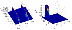
Figure 7: (a) The instability evolution of a symmetric vortex, with $C=0.06,\gamma=0.4$, and $k=0.96$ ($P=1.37$). This unstable vortex does not blow up, but spontaneously transforms into a stable $\mathcal{PT}$-symmetric fundamental soliton. In these panels, the two components of the vortex are juxtaposed, to display the evolution in cross section $m=0$. (b) The instability development in an antisymmetric vortex, for $C=2,\gamma=0.95$, and $k=4$ ($P=66.83$). This unstable mode blows up in its active component, as is common for $\mathcal{PT}$-symmetric systems.

The most important results for the symmetric and antisymmetric vortices, namely, their existence and stability areas in planes of control parameters $\left(k,C\right)$ and $\left(C,P\right)$, are summarized in Fig. 8. For the symmetric OnVs, it is not excluded that, above the triangular existence regions in Fig. 8(a1), and above the existence region in Fig. 8(a2), there exist very strongly unstable vortices which could not be produced by the numerical method.

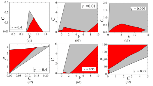
Figure 8: Stability and existence regions for $\mathcal{PT}$-symmetric vortex solitons: (a1) in the $\left(k,C\right)$ plane, and (a2) in the $(P,C)$ plane, for a fixed gain-loss coefficient, $\gamma=0.4$. The variation of $\gamma$ produces small changes in these diagrams (not shown here in detail). (b1,b2,c1) Stability regions of $\mathcal{PT}$-antisymmetric vortex solitons in the $\left(k,C\right)$ plane: (a) for $\gamma=0.01$, (b) for $\gamma=0.95$, and (c1) for $\gamma=0.999$. (c2) The stability region in the $(P,C)$ plane for $\gamma=0.95$. In this case, unlike what happens with symmetric vortices, the stability region strongly changes with the variation of $\gamma$.

Numerical data demonstrate that dependence $P(k)$ for the symmetric and antisymmetric vortices alike is almost exactly given by

$$P_{\mathrm{OnV}}=4P_{\mathrm{FS}}(k),$$ (14)

where $P_{\mathrm{FS}}(k)$ is the respective dependence for the fundamental solitons, see Eq. (11). This relation is naturally explained by the fact that the on-site-centered vortex may be constructed, essentially, as a set of four weakly interacting FSs, with phase shifts $\pi/2$ between adjacent ones Malomed . Relation (14) also helps to map the existence and stability regions for the OnVs in the $\left(C,P\right)$ parameter plane in Figs. 8(a2) and (c2).

Actually, the fact that the symmetric OnVs (at least those which could be produced by the numerical method) exist only at relatively small values of $P$ [at $P<4$ in Fig. 8(a2)] explains that, as stressed above, their instability leads not to the blow-up, but rather to the spontaneous transformation into stable symmetric FSs. It is worthy to note too that the stability region for the symmetric vortices in Fig. 8(a2) is located above the instability area (at larger $P$), while for the symmetric FSs the situation was opposite, cf. Figs. 3(c1) and 3(c2). In this respect, the symmetric vortices resemble antisymmetric FSs, as suggested by the comparison with Fig. 4(d). However, the symmetric OnVs share with symmetric FSs the trend to exist and be stable at values of the total power essentially lower that those at which antisymmetric counterparts are stable, hence the symmetric vortices are more appropriate for the experimental creation.

The stability areas for the antisymmetric OnVs, displayed in Figs. 8(b1)–8(c2), resemble their counterparts shown in Fig. 4 for antisymmetric FSs. In particular, the stability zone tends to extend to $k\rightarrow\infty$, i.e., $P\rightarrow\infty$, except for the case when the gain-loss coefficient, $\gamma$, is very close to its critical value, $1$, see Fig. 8(c1) for $\gamma=0.999$.

The overall dependence of the stability of the vortices on the gain-loss parameter $\gamma$ is characterized by total areas of the stability regions in the $\left(k,C\right)$ plane [see Figs. 8(a1) and 8(b1)–(c1)], which are shown as functions of $\gamma$ in Fig. 9. The drastic difference between these dependences for the symmetric and antisymmetric vortices is obvious.

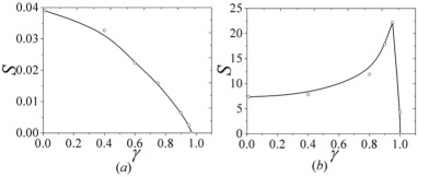
Figure 9: The dependence of the total area of the stability regions in the $\left(k,C\right)$ parameter plane on the gain-loss coefficient, $\gamma$, for the symmetric (a) and antisymmetric (b) vortex solitons. The continuous lines are only guides to the eye.

It was argued above that the fundamental $\mathcal{PT}$-symmetric FS are likely candidates to the role of the system’s ground state. To further verify this conjecture, in Table 1, we compare values of the chemical potential, $\mu$, for a typical set of the control parameters, $(C,\gamma)=(0.05,0.1)$ and $P=1.9$. All the species of discrete solitons considered above exist and are stable at this point (symmetric and antisymmetric FSs and OnVs). The table demonstrates that the symmetric FS has a deep minimum of $\mu$, thus definitely representing the ground state, the three other species being excited states. It is worthy to note too that the lowest excited state is the $\mathcal{PT}$-symmetric vortex, but not the antisymmetric FS. Similar relations between chemical potentials of the four soliton species have been found at other values of the parameters.

Table 1: Chemical potentials of the four coexisting soliton species at $(C,\gamma)=(0.05,0.1)$ and $P=1.9$

Types of solitons	$\mu$
symmetric fundamental soliton	-1.845
symmetric on-site vortex	-1.133
antisymmetric fundamental soliton	0.145
anti-symmetric on-site vortex	0.858

V Conclusion

The objective of this work is to introduce the 2D network of $\mathcal{PT}$-symmetric dimers with the cubic nonlinearity, which support stable $\mathcal{PT}$-symmetric and antisymmetric fundamental and vortical discrete solitons. While the shape of these solitons can be reduced to that of their counterparts in the conservative two-component system (although discrete vortices were not systematically studied even in the conservative system with two linearly coupled components), the study of the stability is crucially important for the consideration of the $\mathcal{PT}$-symmetric system. It has been found that the symmetric FS (fundamental soliton) represents the ground state of the system, and may be stable at lowest values of the total power, thus being the most promising target for the experimental realization. On the contrary, anti-symmetric FS and OnV (on-site-centered vortex) tend to be stable at higher powers. The symmetric OnV represents the first metastable mode above the FS ground state. It also tends to be stable at relatively low powers, and demonstrates remarkable robustness: unlike all the other discrete-soliton species found in this system, unstable symmetric OnVs do not suffer the blow-up, but rather spontaneously transform into stable FSs.

The above analysis did not address mobility of the solitons, but, unlike the 1D version of the system, mobility of 2D discrete solitons is not plausible in the case of the cubic nonlinearity Johansson ; Johansson2 ; Panos . In this connection, it may be interesting to study 2D networks of $\mathcal{PT}$-symmetric dimers with the quadratic nonlinearity, cf. Refs.chi2-1 ; chi2-2 ; chi2-3 , and also Ref. Susanto , where the mobility was demonstrated for 2D discrete solitons in the conservative systems with the quadratic nonlinearity. Another promising extension may deal with 2D systems built of elements which include nonlinear $\mathcal{PT}$-symmetric gain and loss terms Yaro ; Miro .

- (1) Y. V. Kartashov, V. V. Konotop, V. A. Vysloukh, and D. A. Zezyulin, “Guided modes and symmetry breaking supported by localized gain,” in: Spontaneous Symmetry Breaking, Self-Trapping, and Josephson Oscillations, Editor: B. A. Malomed (Springer 2013).
- (2) B. A. Malomed, “Spatial solitons supported by localized gain [Invited],” J. Opt. Soc. Am. B 31, 2460–2475 (2014).
- (3) C. M. Bender and S. Boettcher,“Real spectra in non-Hermitian Hamiltonians having symmetry,” Phys. Rev. Lett. 80, 5243 (1998).
- (4) C. M. Bender, D. C. Brody, and H. F. Jones, “Complex extension of quantum mechanics,” Phys. Rev. Lett.. 89, 270401 (2002).
- (5) A. Ruschhaupt, F. Delgado, and J. G. Muga, “Physical realization of -symmetric potential scattering in a planar slab waveguide,” J. Phys. A 38, L171–L176 (2005).
- (6) K. G. Makris, R. El-Ganainy, and D. N. Christodoulides, “Beam dynamics in symmetric optical lattices,” Phys. Rev. Lett. 100,103904 (2008).
- (7) S. Klaiman, U. Günther, and N. Moiseyev, “Visualization of branch points in -symmetric waveguides,” Phys. Rev. Lett. 101, 080402 (2008).
- (8) A. Guo, G. J. Salamo, M. Volatier-Ravat, V. Aimez, G. Siviloglou, and D. N. Christodoulides, “Observation of -symmetry breaking in complex optical potentials,” Phys. Rev. Lett. 103, 093902 (2009).
- (9) S. Longhi, “Bloch oscillations in complex crystals with symmetry,” Phys. Rev. Lett. 103, 123601 (2009).
- (10) S. Longhi, “Spectral singularities and Bragg scattering in complex crystals,” Phys. Rev. A 81, 022102 (2010).
- (11) K. G. Makris, R. El-Ganainy, D. N. Christodoulides, and Z. H. Musslimani, “ symmetric periodic optical potentials,” Int. J. Theor. Phys. 50, 1019–1041 (2011).
- (12) Y. Li, X. Guo, L. Chen, C. Xu, J. Yang, X. Jiang, and M. Wang, “Coupled mode theory under the parity-time symmetry frame,” J. Lightwave Techn. 31, 2477–2481 (2013).
- (13) A. Regensburger, M. A. Miri, C. Bersch, and J. Näger, “Observation of defect states in -symmetric optical lattices,” Phys. Rev. Lett. 110, 223902 (2013).
- (14) L. Chang, X. Jiang, S. Hua, C. Yang, J. Wen, L. Jiang, G. Li, G. Wang, and M. Xiao, “Parity–time symmetry and variable optical isolation in active-passive-coupled microresonators,” Nature Phot. 8, 524–529 (2014).
- (15) Z. H. Musslimani, K. G. Makris, R. El-Ganainy, and D. N. Christodoulides, “Optical solitons in periodic potentials,” Phys. Rev. Lett. 100, 030402 (2008).
- (16) X. Zhu, H. Wang, L. Zheng, H. Li, and Y. He, “Gap solitons in parity-time complex periodic optical lattices with the real part of superlattices,” Opt. Lett. 36, 2680 (2011).
- (17) F. Kh. Abdullaev, Y. V. Kartashov, V. V. Konotop, and D. A. Zezyulin, “Solitons in -symmetric nonlinear lattices,” Phys. Rev. A 83, 041805(R) (2011).
- (18) H. Li, Z. Shi, X. Jiang and X. Zhu, “Gray solitons in parity-time symmetric potentials,” Opt. Lett. 36, 3290–3292 (2011).
- (19) R. Driben and B. A. Malomed, “Stability of solitons in parity-time-symmetric couplers,” Opt. Lett. 36, 4323–4325 (2011).
- (20) K. Li and P. G. Kevrekidis, “-symmetric oligomers: analytical solutions, linear stability, and nonlinear dynamics,” Phys. Rev. E 83, 066608 (2011).
- (21) A. E. Miroshnichenko, B. A. Malomed, and Y. S. Kivshar, “Nonlinearly -symmetric systems: Spontaneous symmetry breaking and transmission resonances,” Phys. Rev. A 84, 012123 (2011).
- (22) N. V. Alexeeva, I. V. Barashenkov, A. A. Sukhorukov, and Y. S. Kivshar, “Optical solitons in -symmetric nonlinear couplers with gain and loss,” Phys. Rev. A 85, 063837 (2012).
- (23) S. Nixon, L. Ge, and J. Yang, “Stability analysis for solitons in -symmetric optical lattices,” Phys. Rev. A 85, 023822 (2012).
- (24) E. N. Tsoy, S. Sh. Tadjimuratov, and F. Kh. Abdullaev, “Beam propagation in gain-loss balanced waveguides,” Opt. Commun. 285, 3441–3444 (2012).
- (25) N. V. Alexeeva, I. V. Barashenkov, A. A. Sukhorukov, and Y. S. Kivshar, “Optical solitons in -symmetric nonlinear couplers with gain and loss,” Phys. Rev. A 85 063837 (2012).
- (26) K. Li , P. G. Kevrekidis, B. A. Malomed, and U. Günther, “Nonlinear -symmetric plaquettes,” J. Phys. A 45, 444021 (2012).
- (27) K. Li, D. A. Zezyulin, V. V. Konotop, and P. G. Kevrekidis, “Parity-time-symmetric optical coupler with birefringent arms,” Phys. Rev. A 87, 033812 (2013).
- (28) T. Mayteevarunyoo, B. A. Malomed, and A. Roeksabutr, “Solvable model for solitons pinned to a parity-time-symmetric dipole,” Phys. Rev. E 88, 022919 (2013).
- (29) I. V. Barashenkov, G. S. Jackson, and S. Flach, “Blow-up regimes in the -symmetric coupler and the actively coupled dimer,” Phys. Rev. A 88, 053817 (2013).
- (30) G. Burlak and B. A. Malomed, “Stability boundary and collisions of two-dimensional solitons in -symmetric couplers with the cubic-quintic nonlinearity,” Phys. Rev. E 88, 062904 (2013).
- (31) J. Pickton and H. Susanto, “Integrability of -symmetric dimers,” Phys. Rev. A 88, 063840 (2013).
- (32) A. S. Rodrigues, K. Li, V. Achilleos, P. G. Kevrekidis, D. J. Frantzeskakis, and C. M. Bender, “ -symmetric double-well potentials revisited: bifurcations, stability and dynamics,” Rom. Rep. Phys. 65, 5–26 (2013).
- (33) Y. Lumer, Y. Plotnik, M. C. Rechtsman, and M. Segev, “Nonlinearly induced transition in photonic systems,” Phys. Rev. Lett. 111, 263901 (2013).
- (34) J. Yang, “Symmetry breaking of solitons in one-dimensional parity-time-symmetric optical potentials,” Opt. Lett. 30, 5547–5550 (2014).
- (35) H. Li, X. Zhu, Z. Shi, B. A. Malomed, T. Lai, and C. Lee, “Bulk vortex and horseshoe surface modes in parity-time-symmetric media,” Phys. Rev. A 89, 053811 (2014).
- (36) Y. V. Kartashov, B. A. Malomed, and L. Torner, “Unbreakable symmetry of solitons supported by inhomogeneous defocusing nonlinearity,” Opt. Lett. 39, 5641–5644 (2014).
- (37) C. E. Rüter, K. G. Makris, R. El-Ganainy, D. N. Christodoulides, M. Segev,and D. Kip, “Observation of parity-time symmetry in optics,” Nature Physics 6, 192 (2010).
- (38) S. V. Dmitriev, S. V. Suchkov, A. A. Sukhorukov, and Y. S. Kivshar, “Scattering of linear and nonlinear waves in a waveguide array with a -symmetric defect,” Phys. Rev. A 84, 013833 (2011).
- (39) S. V. Suchkov, B. A. Malomed, S. V. Dmitriev, and Y. S. Kivshar, “Solitons in a chain of parity-time-invariant dimers,” Phys. Rev. E 84, 046609 (2011).
- (40) S. V. Suchkov, A. A. Sukhorukov, S. V. Dmitriev, and Y. S. Kivshar, “Scattering of the discrete solitons on the -symmetric defects,” Europhys. Lett. 100, 54003 (2012).
- (41) S. V. Suchkov, S. V. Dmitriev, B. A. Malomed, and Y. S. Kivshar, “Wave scattering on a domain wall in a chain of -symmetric couplers,” Phys. Rev. A 85, 033835 (2012).
- (42) D. A. Zezyulin and V. V. Konotop, “Nonlinear modes in finite-dimensional -symmetric systems,” Phys. Rev. Lett. 108, 213906 (2012).
- (43) V. V. Konotop, D. E. Pelinovsky, and D. A. Zezyulin, “Discrete solitons in -symmetric lattices,” EPL 100, 56006 (2012).
- (44) D. Leykam, V. V Konotop, and A. S. Desyatnikov, “Discrete vortex solitons and parity time symmetry,” Opt. Lett. 38, 371 (2013).
- (45) N. Lazarides and G. P. Tsironis, “Gain-driven discrete breathers in-symmetric nonlinear metamaterials,” Phys. Rev. Lett. 110, 053901 (2013).
- (46) P. G. Kevrekidis, D. E. Pelinovsky, and D. Y. Tyugin, “Nonlinear stationary states in -symmetric lattices,” SIAM J. Appl. Dyn. Syst. 12, 1210–1236 (2013).
- (47) X. Zhang, J. Chai, J. Huang, Z. Chen, Y. Li, and B. A. Malomed, “Discrete solitons and scattering of lattice waves in guiding arrays with a nonlinear -symmetric defect,” Opt. Exp. 22, 6055 (2014).
- (48) C. H. Liang, D. D. Scott, and Y. N. Joglekar, “ restoration via increased loss and gain in the -symmetric Aubry-André model,” Phys. Rev. A 89, 030102(R) (2014).
- (49) J. S. Aitchison, D. C. Hutchings, J. U. Kang, G. I. Stegeman, and A. Villeneuve, “The nonlinear optical properties of AlGaAs at the half band gap,” IEEE J. Quantum Electron. 33, 341 (1997).
- (50) A. Yariv and P. Yeh, Photonics: Optical Electronics in Modern Communications (Oxford University Press 2007).
- (51) Z. Mai, S. Fu, J. Wu, and Y. Li, “Discrete Solitons in Waveguide Arrays with Long-Range Linearly Coupled Effect,” J. Phys. Soc. Jpn. 83, 034404 (2014).
- (52) G. Herring, P. G. Kevrekidis, B. A. Malomed, R. Carretero-González, and D. J. Frantzeskakis, “Symmetry breaking in linearly coupled dynamical lattices,” Phys. Rev. E 76, 066606 (2007).
- (53) P. G. Kevrekidis, The Discrete Nonlinear Schrödinger Equation: Mathematical Analysis, Numerical Computations, and Physical Perspectives (Springer 2009).
- (54) B. A. Malomed and P. G. Kevrekidis, “Discrete vortex solitons,” Phys. Rev. E, 64, 026601 (2011).
- (55) N. G. Vakhitov, A. A. Kolokolov, “Stationary solutions of the wave equation in a medium with nonlinearity saturation,” Radiophys. Quantum Electron., 16, 783–789 (1973).
- (56) L. Bergé, “Wave collapse in physics: principles and applications to light and plasma waves,” Phys. Rep. 303, 259–370 (1998).
- (57) W. Z. Bao and Q. Du, “Computing the ground state solution of Bose-Einstein condensates by a normalized gradient flow,” SIAM J. Sci. Comp. 25, 1674–1697 (2004).
- (58) M. L. Chiofalo, S. Succi, and M. P. Tosi, “Ground state of trapped interacting Bose-Einstein condensates by an explicit imaginary-time algorithm,” Phys. Rev. E 62, 7438–7444 (2000).
- (59) R. A. Vicencio and M. Johansson, “Discrete soliton mobility in two-dimensional waveguide arrays with saturable nonlinearity,” Phys. Rev. E 73, 046602 (2006).
- (60) M. Öster and M. Johansson, “Stability, mobility and power currents in a two-dimensional model for waveguide arrays with nonlinear coupling,” Physica D 238, 88–99 (2009).
- (61) H. Susanto, P. G. Kevrekidis, R. Carretero-González, B. A. Malomed, and D. J. Frantzeskakis, “Mobility of discrete solitons in quadratically nonlinear media,” Phys. Rev. Lett. 99, 214103 (2007).
- (62) F. C. Moreira F. Kh. Abdullaev, V. V. Konotop, and A. V. Yulin, “Localized modes in media with -symmetric localized potential,” Phys. Rev. A 86, 053815 (2012).
- (63) F. C. Moreira, V. V. Konotop, and B. A. Malomed, “Solitons in -symmetric periodic systems with the quadratic nonlinearity,” Phys. Rev. A 87, 013832 (2013).
- (64) K. Li, D. A. Zezyulin, P. G. Kevrekidis, V. V. Konotop, and F. Kh. Abdullaev, “-symmetric coupler with nonlinearity,” Phys. Rev. A 88, 053820 (2013).