Local Asymptotic Normality of the spectrum of high-dimensional spiked F-ratios

Abstract

We consider two types of spiked multivariate F distributions: a scaled distribution with the scale matrix equal to a rank-one perturbation of the identity, and a distribution with trivial scale, but rank-one non-centrality. The norm of the rank-one matrix (spike) parameterizes the joint distribution of the eigenvalues of the corresponding F matrix. We show that, for a spike located above a phase transition threshold, the asymptotic behavior of the log ratio of the joint density of the eigenvalues of the F matrix to their joint density under a local deviation from this value depends only on the largest eigenvalue $\lambda_{1}$. Furthermore, $\lambda_{1}$ is asymptotically normal, and the statistical experiment of observing all the eigenvalues of the F matrix converges in the Le Cam sense to a Gaussian shift experiment that depends on the asymptotic mean and variance of $\lambda_{1}$. In particular, the best statistical inference about a sufficiently large spike in the local asymptotic regime is based on the largest eigenvalue only. As a by-product of our analysis, we establish joint asymptotic normality of a few of the largest eigenvalues of the multi-spiked F matrix when the corresponding spikes are above the phase transition threshold.
Key words: Spiked F-ratio, Local Asymptotic Normality, multivariate F distribution, phase transition, super-critical regime, asymptotic normality of eigenvalues, limits of statistical experiments.

1 Introduction

In this paper we establish the Local Asymptotic Normality (LAN) of the statistical experiments of observing the eigenvalues of the F-ratio, $B^{-1}A,$ of two high-dimensional independent Wishart matrices, $A$ and $B$. We consider two situations. First, both $A$ and $B$ are central Wisharts with dimensionality and degrees of freedom that grow proportionally, and with the covariance parameters that differ by a matrix of rank one. Second, $A$ and $B$ have the same covariance parameter, but $A$ is a non-central Wishart with the non-centrality parameter of rank one. In both cases, the joint distribution of the eigenvalues of $B^{-1}A$ depends on the norm of the rank-one matrix, which we call a spike. We find that the considered statistical experiments are LAN under a local parameterization of the spike when the locality is above a phase transition threshold.

Many classical multivariate statistical tests are based on the eigenvalues of F-ratio matrices. For example, all tests of the equality of two covariance matrices and of the general linear hypothesis in the Multivariate Linear Model described in Muirhead’s (1982) chapters 8 and 10 are of this form. Contemporaneous statistical applications often require the dimensionality of the F-ratio and its degrees of freedom be large and comparable. Therefore, we consider the asymptotic regime where the dimensionality and the degrees of freedom diverge to infinity at the same rate.

Our requirement that the parameters of the two Wisharts differ by a rank-one matrix can be linked to situations where the alternative hypothesis is characterized by the presence of one factor or signal, which is absent from the data under the null. Inference conditional on factors requires considering non-central F-ratios, whereas the unconditional inference leads to F-ratios with unequal covariances.

The main result of this paper can be summarized as follows. We show that the asymptotic behavior of the log ratio of the joint density of the eigenvalues of $B^{-1}A,$ which corresponds to a sufficiently large value of the spike, to their joint density under a local deviation from this value depends only on the largest eigenvalue $\lambda_{1}$. Furthermore, $\lambda_{1}$ is asymptotically normal, and the statistical experiment of observing all the eigenvalues of $B^{-1}A$ converges in the Le Cam sense to a Gaussian shift experiment that depends on the asymptotic mean and variance of $\lambda_{1}$. In particular, the best statistical inference about a sufficiently large spike in the local asymptotic regime is based on the largest eigenvalue only.

We derive an explicit formula for the phase transition threshold demarcating the area of the sufficiently large spikes. In a general framework, where the parameters of $A$ and $B$ may differ by a matrix $\Delta$ of a finite rank, we show that, when the norm of $\Delta$ is below the threshold, any finite number of the largest eigenvalues of $B^{-1}A$ almost surely converge to the upper boundary of the support of the limiting spectral distribution of $B^{-1}A,$ derived by Wachter (1980). In contrast, when $m$ of the largest eigenvalues of $\Delta$ are above the threshold, we find that the $m$ of the largest eigenvalues of $B^{-1}A$ almost surely converge to locations strictly above the upper boundary of Wachter’s distribution, and that their local fluctuations about these limits are asymptotically jointly normal.

In a setting of two independent and not necessarily normal samples, the phase transition phenomenon has been studied in Nadakuditi and Silverstein (2010). They obtain a formula for the threshold, and establish the almost sure limits of the $m$ largest eigenvalues for the case where $\Delta$ describes the difference between covariance matrices of the two samples. The limiting distribution of fluctuations above the threshold is described in their paper as an open problem. Our paper solves this problem for the case of two normal samples.

The phase transition phenomenon for a single Wishart matrix has also been a subject of active recent research. Baik et al (2005) study the joint distributions of a few of the largest eigenvalues of complex Wisharts with spiked covariance parameters. They derive the asymptotic distributions of a few of the largest eigenvalues, which turn out to be different depending on whether the sizes of the corresponding spikes are below, at, or above a phase transition threshold, the situations often referred to as the sub-critical, critical, and super-critical regimes.

Similar transition takes place for real Wisharts. Paul (2007) establishes asymptotic normality of the fluctuations of a few of the largest eigenvalues in the super-critical regime of the real case. Féral and Péché (2009), Benaych-Georges et al (2011) and Bao et al (2014a) show that the fluctuations in the sub-critical real case have the Tracy-Widom distribution, while Mo (2012) and Bloemendal and Viràg (2011, 2013) establish the asymptotic distribution of a different type in the critical regime. In a setting of two normal samples, Bao et al (2014b) study the almost sure limits of the sample canonical correlations when the population canonical correlations are below and when they are above a phase transition threshold.

Our results on the joint asymptotic normality of the largest eigenvalues in the super-critical regime for F-ratios can be used to make statistical inference about the eigenvalues of the “ratio” of the population covariances of $A$ and $B$, or the eigenvalues of the non-centrality parameter of $A$. The estimates of these eigenvalues play important role in MANOVA and the discriminant analysis, and can also be used in constructing modified model selection criteria as discussed in Sheena et al (2004). Further, they may be important in as diverse applications as constructing genetic selection indices and describing a degree of financial turbulence (see Hayes and Hill (1981), and Kritzman and Li (2010)).

We expect that our asymptotic normality results can be extended to the case of the “ratio” of two sample covariance matrices constructed from non-normal samples. In the one-sample case, such an extension of Paul’s (2007) asymptotic normality results has been done in Bai and Yao (2008). In this paper, we focus on normal data. This focus is dictated by our main goal: establishing the LAN property of the statistical experiments of observing the eigenvalues of $B^{-1}A$. To reach this goal, we derive an asymptotic approximation to a log likelihood process by representing it in the form of a contour integral, and applying the Laplace approximation method. The explicit form of the joint distribution of the eigenvalues of $B^{-1}A$ is known only in the normal case, and we need such an explicit form for our analysis.

A decision-theoretic approach to the finite sample estimation of the eigenvalues of the “ratio” of the population covariances of $A$ and $B$, or the eigenvalues of the non-centrality parameter of $A$ was taken in many previous studies (see Sheena et al (2004), Bilodeau and Srivastava (1992), and references therein). In one of the first such studies, Muirhead and Verathaworn (1985) explain that the ideal decision-theoretic approach that directly analyzes expected loss with respect to the joint distribution of the eigenvalues of $B^{-1}A$ “does not seem feasible due primarily to the complexity of the distribution of the ordered latent roots…” Instead, they focus on deriving an optimal estimator from a particular class.

Our LAN result makes possible an asymptotic implementation of the ideal decision-theoretic approach. We overcome the complexity of the joint distribution of the eigenvalues by using a tractable contour integral representation of the log likelihood process, which was obtained in the single-spike case by Dharmawansa and Johnstone (2014). In the multiple-spike case, a similar representation involves multiple contour integrals (see Passemier et al (2014)). An asymptotic analysis of such a multiple integral requires a substantial additional effort, and we leave it for future research.

It is interesting to contrast the LAN result in the super-critical regime with the asymptotic behavior of the log likelihood ratio in the case of a sub-critical spike. In a separate research effort, we follow Onatski et al (2013), who analyze the log likelihood ratio in the sub-critical regime for the case of a single Wishart matrix, to show that the experiment of observing the eigenvalues of $B^{-1}A$ in the sub-critical regime is not of the LAN type. Furthermore, the log-likelihood process turns out to depend only on a smooth functional of the empirical distribution of all the eigenvalues of $\Sigma^{-1}A,$ so that asymptotically efficient inference procedures may ignore the information contained in $\lambda_{1}$ altogether. The results of this sub-critical analysis will be published elsewhere.

The rest of the paper is structured as follows. In the next section, we describe our setting. In Section 3, we derive the almost sure limits of a few of the largest eigenvalues of the F-ratio. In Section 4, we establish the asymptotic normality of the eigenvalue fluctuations in the super-critical regime. In Section 5, we derive an asymptotic approximation to the joint distribution of the eigenvalues of $B^{-1}A$ for the special case of a single super-critical spike. In Section 6, we show that the likelihood ratio in the local parameter space is asymptotically equivalent to a centered and scaled largest eigenvalue, and establish the LAN property. Section 7 concludes.

2 Setup

Suppose that

$$A\sim W_{p}\left(n_{1}+k,\Sigma_{1},\Omega_{1}\right)\text{ \qquad and }\qquad B\sim W_{p}\left(n_{2},\Sigma_{2}\right)$$

are independent non-central and central Wishart matrices respectively. For the non-centrality parameter $\Omega_{1}$, we use a symmetric version of the definition in Muirhead (1982, p. 442). That is, if $Z$ is an $n\times p$ matrix distributed as $N\left(M,I_{n}\otimes\Sigma\right),$ then $Z^{\prime}Z\sim W_{p}\left(n,\Sigma,\Omega\right)$ with the non-centrality parameter $\Omega=\Sigma^{-1/2}M^{\prime}M\Sigma^{-1/2}$. We will consider two different settings for the parameters $\Sigma_{1},\Sigma_{2},$ and $\Omega_{1}$.

Setting 1

(Spiked covariance) $\Sigma_{2}=\Sigma,$ $\Sigma_{1}=\Sigma^{1/2}\left(I_{p}+VhV^{\prime}\right)\Sigma^{1/2},$ and $\Omega_{1}=0.$ Here $\Sigma^{1/2}$ is the symmetric square root of a positive definite matrix $\Sigma;$ $V$ in a $p\times k$ matrix of nuisance parameters with orthonormal columns, and $h=\mathrm{diag}\left\{h_{1},...,h_{k}\right\}$ is the diagonal matrix of the “covariance spikes” with $h_{1}>...>h_{k}$.

Setting 2

(Spiked non-centrality) $\Sigma_{2}=\Sigma,$ $\Sigma_{1}=\Sigma,$ and $\Omega_{1}=\left(n_{1}+k\right)VhV^{\prime},$ where $\Sigma,$ $V,$ and $h$ are as defined above, but $h_{j}$ with $j=1,...,k$ are interpreted as “non-centrality spikes.”

We are interested in the behavior of the eigenvalues of

$$\mathbf{F}\equiv\left(B/n_{2}\right)^{-1}A/n_{A},$$

where

$$n_{A}=n_{1}+k,$$

as $n_{1},n_{2},$ and $p$ grow so that $p/n_{1}\rightarrow c_{1}$ and $p/n_{2}\rightarrow c_{2}$ with $0<c_{i}<1,$ while $k$, the number of spikes, remains fixed. In what follows, we will assume that $\Sigma=I_{p}$. This assumption is without loss of generality because the eigenvalues of $\mathbf{F}$ do not change under the transformation $A\mapsto\Sigma^{-1/2}A\Sigma^{-1/2},$ $B\mapsto\Sigma^{-1/2}B\Sigma^{-1/2}$.

It is convenient to think of $A/n_{A}$ as a sample covariance matrix $XX^{\prime}/n_{A}$ of the sample $X$ having the factor structure

$$X=V\mathcal{F}^{\prime}+\varepsilon$$ (1)

with $V,\mathcal{F},$ and $\varepsilon$ playing the roles of the factor loadings, factors, and idiosyncratic terms, respectively. Matrices $\mathcal{F}$ and $\varepsilon$ are mutually independent, and independent from $B$. The distribution of $\varepsilon$ is $N\left(0,I_{p}\otimes I_{n_{A}}\right),$ and the distribution of $\mathcal{F}$ depends on the setting. For Setting 1, $\mathcal{F}\sim N\left(0,I_{p}\otimes h\right),$ whereas for Setting 2, $\mathcal{F}$ is a deterministic matrix such that $\mathcal{F}^{\prime}\mathcal{F}/n_{A}=h$. With this interpretation, Settings 1 and 2 describe, respectively, distributions which are unconditional and conditional on the factors. In both cases the spike parameters $h_{j},$ $j=1,...,k,$ measure the factors’ variability.

We would like to introduce a convenient representation of the eigenvalues of $\mathbf{F}$, that we will denote as $\lambda_{p1}\geq...\geq\lambda_{pp}$. First, note that $\lambda_{pj},$ $j=1,...,p$, are invariant with respect to the simultaneous transformations

$$A\mapsto UAU^{\prime}\equiv n_{A}\tilde{H}\text{ \qquad and }\qquad B\mapsto UBU^{\prime}\equiv n_{2}E,$$ (2)

where $U$ is a random matrix uniformly distributed over the orthogonal group $\mathcal{O}\left(p\right)$. Under the assumption that $\Sigma=I_{p},$ matrix $n_{2}E$ is distributed as $W_{p}\left(n_{2},I_{p}\right)$ and is independent from $\tilde{H}$. Matrix $\tilde{H}$ has the form $\tilde{X}\tilde{X}^{\prime}/n_{A},$ where

$$\tilde{X}=\tilde{V}\mathcal{F}^{\prime}+\tilde{\varepsilon}$$

with $\tilde{\varepsilon}\sim N\left(0,I_{p}\otimes I_{n_{A}}\right)$ independent from $\tilde{V}$, and $\tilde{V}$ being a random $p\times k$ matrix uniformly distributed on the Stiefel manifold of orthogonal $k$-frames in $\mathbb{R}^{p}.$ We can think of $\tilde{V}$ as having the form

$$\tilde{V}=v\left(v^{\prime}v\right)^{-1/2}\equiv vW_{v}^{-1/2},$$

where $v\sim N\left(0,I_{p}\otimes I_{k}\right)$ and $W_{v}\equiv v^{\prime}v$ is Wishart $W_{k}\left(p,I_{k}\right).$

Further, let $O_{\mathcal{F}}\in\mathcal{O}\left(n_{A}\right)$ be such that the submatrix of its first $k$ columns equals $\mathcal{F}\left(\mathcal{F}^{\prime}\mathcal{F}\right)^{-1/2}$, and let $\hat{X}=\tilde{X}O_{\mathcal{F}}$. Clearly,

$$\tilde{H}=\tilde{X}\tilde{X}^{\prime}/n_{A}=\hat{X}\hat{X}^{\prime}/n_{A},$$ (3)

and matrix $\hat{X}$ has the form

$$\hat{X}=vW_{v}^{-1/2}h^{1/2}W_{\mathcal{F}}^{1/2}+\hat{\varepsilon},$$

where $v,W_{\mathcal{F}}$ and $\hat{\varepsilon}$ are mutually independent and independent from $E;$ $\hat{\varepsilon}\sim N\left(0,I_{p}\otimes I_{n_{A}}\right)$; and the distribution of $W_{\mathcal{F}}$ depends on the setting. For Setting 1, $W_{\mathcal{F}}\sim W_{k}\left(n_{A},I_{k}\right),$ whereas for Setting 2, $W_{\mathcal{F}}=n_{A}I_{k}$.

Finally, let us denote the submatrix of the first $k$ columns of $\hat{\varepsilon}$ as $u.$ Then

$$\hat{X}\hat{X}^{\prime}=\xi\xi^{\prime}+n_{1}H,$$ (4)

where $n_{1}H\sim W_{p}\left(n_{1},I_{p}\right),$ $H$ and $\xi\xi^{\prime}$ are mutually independent, and independent from $E,$ and

$$\xi=vW_{v}^{-1/2}h^{1/2}W_{\mathcal{F}}^{1/2}+u.$$ (5)

Using (2), (3), and (4), we obtain the convenient representation for the eigenvalues, announced above. Let $\hat{x}_{p1}\geq...\geq\hat{x}_{pp}$ be the roots of the equation

$$\det\left(\xi\xi^{\prime}/n_{1}+H-xE\right)=0.$$ (6)

Then

$$\lambda_{pj}=n_{1}\hat{x}_{pj}/\left(n_{1}+k\right).$$ (7)

This representation is convenient because the roots of (6) can be viewed and analyzed as perturbations of the roots of equation $\det\left(H-xE\right)=0$ caused by adding the low-rank matrix $\xi\xi^{\prime}/n_{1}$ to $H$.

If $x\in\mathbb{R}$ is such that $H-xE$ is invertible, then

$$\left(\xi\xi^{\prime}/n_{1}+H-xE\right)^{-1}=S-S\xi\left(I_{k}+\xi^{\prime}S\xi/n_{1}\right)^{-1}\xi^{\prime}S/n_{1},$$

where $S\equiv\left(H-xE\right)^{-1}$. Therefore, if $x$ is a root of the equation

$$\det\left(I_{k}+\xi^{\prime}\left(H-xE\right)^{-1}\xi/n_{1}\right)=0,$$ (8)

then it also solves (6), and hence, the asymptotic behavior of the roots of (6) can be inferred from that of the random matrix-valued function

$$M\left(x\right)=\xi^{\prime}\left(H-xE\right)^{-1}\xi/n_{1}.$$ (9)

This is the main idea of the analysis in the next section of the paper.

3 Almost sure limits of the largest eigenvalues

Let $\mathbf{n}\equiv\left(n_{1},n_{2}\right)$ and $\mathbf{c}\equiv\left(c_{1},c_{2}\right)$. We will denote the asymptotic regime where $n_{1},n_{2},$ and $p$ grow so that $p/n_{1}\rightarrow c_{1}$ and $p/n_{2}\rightarrow c_{2}$ with $c_{j}\in\left(0,1\right)$ as $p,\mathbf{n}\rightarrow_{\mathbf{c}}\infty$. As follows from Wachter’s (1980) work, as $p,\mathbf{n}\rightarrow_{\mathbf{c}}\infty$, the empirical distribution of the eigenvalues of $E^{-1}H$ converges in probability to the distribution with density

$$\frac{1-c_{2}}{2\pi}\frac{\sqrt{\left(b_{+}-\lambda\right)\left(\lambda-b_{-}\right)}}{\lambda\left(c_{1}+c_{2}\lambda\right)}\mathbf{1}\left\{b_{-}\leq\lambda\leq b_{+}\right\}.$$ (10)

The upper and the lower boundaries of the support of this density are

$$b_{\pm}=\left(\frac{1\pm r}{1-c_{2}}\right)^{2},\text{ where }r=\sqrt{c_{1}+c_{2}-c_{1}c_{2}}\text{.}$$

The results of Silverstein and Bai (1995) and Silverstein (1995) show that the empirical distribution converges not only in probability, but also almost surely (a.s.). Furthermore, as follows from Theorem 1.1 of Bai and Silverstein (1998), the largest eigenvalue of $E^{-1}H$ a.s. converges to $b_{+}$.

The latter convergence, together with (7) and Weyl’s inequalities for the eigenvalues of a sum of two Hermitian matrices (see Theorem 4.3.7 in Horn and Johnson (1985)), imply that the $k+1$-th largest eigenvalue of $\mathbf{F,}$ $\lambda_{p,k+1}$, a.s. converges to $b_{+}$. Those of the $k$ largest eigenvalues that remain separated from $b_{+}$ as $p,\mathbf{n}\rightarrow_{\mathbf{c}}\infty$, must correspond to solutions of (8). Below, we study these solutions in detail.

Lemma 1

For any $x>b_{+},$ as $p,\mathbf{n}\rightarrow_{\mathbf{c}}\infty$,

$$\frac{1}{p}\operatorname*{tr}\left[\left(H-xE\right)^{-1}\right]\overset{a.s.}{\rightarrow}m_{x}(0)\text{ and}$$ (11)

$$\frac{1}{p}\operatorname*{tr}\left[\frac{\mathrm{d}}{\mathrm{d}x}\left(H-xE\right)^{-1}\right]\overset{a.s.}{\rightarrow}\frac{\mathrm{d}}{\mathrm{d}x}m_{x}(0),$$ (12)

where $m_{x}(0)=\lim_{z\rightarrow 0}m_{x}(z),$ and $m_{x}(z)\in\mathbb{C}^{+}$ is analytic in $z\in\mathbb{C}^{+},$ and satisfies equation

$$z-\frac{1}{1+c_{1}m_{x}\left(z\right)}=-\frac{1}{m_{x}\left(z\right)}-\frac{x}{1-c_{2}xm_{x}\left(z\right)}.$$ (13)

Proof: Let $x\in\mathbb{R}$ be such that $x>b_{+},$ and let $F_{x}(\lambda)$ be the empirical distribution function of the eigenvalues of $H-xE$. For any $z\in\mathbb{C}^{+},$ let

$$\hat{m}_{x}\left(z\right)=\int\left(\lambda-z\right)^{-1}\mathrm{d}F_{x}(\lambda)$$

be the Stieltjes transform of $F_{x}(\lambda)$. Note that matrix $H-xE$ can be represented in the form $YTY^{\prime}/p,$ where $Y\sim N\left(0,I_{p}\otimes I_{n_{1}+n_{2}}\right)$ and $T$ is a diagonal matrix with the first $n_{1}$ and the last $n_{2}$ diagonal elements equal to $p/n_{1}$ and $-xp/n_{2},$ respectively. Therefore, by Theorem 1.1 of Silverstein and Bai (1995), for any $z\in\mathbb{C}^{+},$ $\hat{m}_{x}\left(z\right)$ a.s. converges to $m_{x}\left(z\right)\in\mathbb{C}^{+},$ which is an analytic function in the domain $z\in\mathbb{C}^{+}$ that solves the functional equation (13).

By Theorem 1.1 of Bai and Silverstein (1998), the largest eigenvalue of $E^{-1}H$ a.s. converges to $b_{+}$. Therefore, for any $x>b_{+},$ the largest eigenvalue of $H-xE$ is a.s. asymptotically bounded away from the positive semi-axis. Hence, $\hat{m}_{x}\left(z\right)$ is analytic and bounded in a small disc $D$ around $z=0$ for all sufficiently large $p$ and $\mathbf{n},$ a.s. By Vitali’s theorem (see Titchmarsh (1960), p.168), $\hat{m}_{x}\left(z\right)$ is a.s. converging to an analytic function in $D$. Since, in $D\cap\mathbb{C}^{+}$, the limiting function is $m_{x}\left(z\right),$ we have

$$\frac{1}{p}\operatorname*{tr}\left[\left(H-xE\right)^{-1}\right]=\hat{m}_{x}\left(0\right)\overset{a.s.}{\rightarrow}m_{x}\left(0\right),$$

where $m_{x}(0)=\lim_{z\rightarrow 0}m_{x}(z)$. Further, $\frac{1}{p}\operatorname*{tr}\left[\left(H-\zeta E\right)^{-1}\right]$ is an analytic bounded function of $\zeta$ in a small disk $D_{x}$ around $x,$ for all sufficiently large $p$ and $\mathbf{n},$ a.s. Therefore, by Vitali’s theorem its a.s. limit $f(\zeta)$ is analytic in $D_{x},$ and

$$\frac{1}{p}\operatorname*{tr}\left[\frac{\mathrm{d}}{\mathrm{d}\zeta}\left(H-\zeta E\right)^{-1}\right]\overset{a.s.}{\rightarrow}\frac{\mathrm{d}}{\mathrm{d}\zeta}f(\zeta)$$

in $D_{x}.$ On the other hand, we know that $f(\zeta)=m_{\operatorname{Re}\zeta}(0)$ for $\zeta$ from $D_{x}$. Therefore, we have (12).$\square$

Lemma 2

For any $x>b_{+}$, as $p,\mathbf{n}\rightarrow_{\mathbf{c}}\infty$,

$$\left\|M\left(x\right)-\left(h+c_{1}I_{k}\right)\frac{1}{p}\operatorname*{tr}\left[\left(H-xE\right)^{-1}\right]\right\|\overset{a.s.}{\rightarrow}0\text{ and}$$

$$\left\|\frac{\mathrm{d}}{\mathrm{d}x}M\left(x\right)-\left(h+c_{1}I_{k}\right)\frac{1}{p}\operatorname*{tr}\left[\frac{\mathrm{d}}{\mathrm{d}x}\left(H-xE\right)^{-1}\right]\right\|\overset{a.s.}{\rightarrow}0,$$

where $\left\|\cdot\right\|$ denotes the spectral norm.

Proof: This convergences follow from (5), (9), and Lemma 3 stated below.$\square$

Lemma 3

Let $C$ be a random $p\times p$ matrix, independent from $u$ and $v$, which are as defined in Section 2, and such that $p\left\|C\right\|$ is bounded for all sufficiently large $p,$ a.s. Then, as $p\rightarrow\infty$,

$$\left\|v^{\prime}Cv-\left(\operatorname*{tr}C\right)I_{k}\right\|\overset{a.s.}{\rightarrow}0\text{ and }\left\|v^{\prime}Cu\right\|\overset{a.s.}{\rightarrow}0.$$

Proof: This lemma follows from the Borel-Cantelli lemma, and the upper bounds on the fourth moments of the entries $v^{\prime}Cv-\left(\operatorname*{tr}C\right)I_{k}$ and $v^{\prime}Cu$ established by Lemma 2.7 of Bai and Silverstein (1998).$\square$

Lemma 4

(i) For any $\varepsilon>0,$ the $k$ eigenvalues of $M\left(x\right)$ are strictly increasing functions of $x\in\left(b_{+}+\varepsilon,\infty\right)$ for sufficiently large $p$ and $\mathbf{n}$, a.s.; (ii) $m_{x}(0)$ is a strictly increasing, continuous function of $x\in\left(b_{+},\infty\right)$; (iii) $\lim_{x\rightarrow\infty}m_{x}(0)=0$, and $\lim_{x\downarrow b_{+}}m_{x}(0)\left(h_{i}+c_{1}\right)<-1$ if and only if $h_{i}>\bar{h},$ where

$$\bar{h}=\frac{c_{2}+r}{1-c_{2}}.$$

Proof: Let $\mu_{1}\in\left(0,\infty\right)$ be the largest eigenvalue of $E^{-1}H.$ For any $x_{1}>x_{2}>\mu_{1},$ matrix $\left(x_{1}E-H\right)^{-1}-\left(x_{2}E-H\right)^{-1}$ is negative definite, a.s. Part (i) follows from this, from the definition (9), and from the fact that $\mu_{1}\overset{a.s.}{\rightarrow}b_{+}.$ Part (i) together with Lemmas 1 and 2 imply that $m_{x}(0)$ is increasing on $\left(b_{+},\infty\right).$ It is strictly increasing because, otherwise, (13) would not be satisfied for some $z\in\mathbb{C}^{+}$ that are sufficiently close to zero. The continuity follows from the analyticity of $m_{x}(0)$ established in the proof of Lemma 1. Finally, $\lim_{x\rightarrow\infty}m_{x}(0)=0$ is implied by (ii) and (11). Equation (13) implies that

$$\lim_{x\downarrow b_{+}}m_{x}(0)=\frac{c_{2}-1}{\left(r+1\right)r},$$

which, in its turn, implies the second statement of (iii).$\square$

Let $\hat{x}_{p1}\geq...\geq\hat{x}_{pk}$ be the solutions of equation (8). By Lemmas 1, 2, and 4, if

$$h_{1}>...>h_{m}>\bar{h}>h_{m+1}>...>h_{k},$$ (14)

then $\hat{x}_{pi}\overset{a.s.}{\rightarrow}x_{i},$ where $x_{i},$ $i=1,...,m,$ are such that

$$1+\left(h_{i}+c_{1}\right)m_{x_{i}}(0)=0$$ (15)

and $m_{x_{i}}(0)$ satisfies (13) with $x$ replaced by $x_{i}.$ In particular,

$$\frac{1}{1+c_{1}m_{x_{i}}(0)}-\frac{1}{m_{x_{i}}(0)}-\frac{x_{i}}{1-c_{2}x_{i}m_{x_{i}}(0)}=0.$$ (16)

Combining (15) and (16), we obtain

$$\frac{1}{h_{i}}+1-\frac{x_{i}}{h_{i}+c_{1}+c_{2}x_{i}}=0,$$

which implies that

$$x_{i}=\frac{\left(h_{i}+c_{1}\right)\left(h_{i}+1\right)}{h_{i}-c_{2}\left(h_{i}+1\right)}.$$ (17)

By (7), $n_{1}\hat{x}_{pi}/\left(n_{1}+k\right),$ $i=1,...,m$, must be the $m$ largest eigenvalues of $\mathbf{F},$ and thus, $x_{i},$ $i=1,...,m,$ describe their a.s. limits. Since there are only $m$ roots of (8) that are asymptotically separated from $b_{+}$ and are located above $b_{+},$ the other $k-r$ of the largest eigenvalues of $\mathbf{F}$ must a.s. converge to $b_{+}$. To summarize, the following proposition holds.

Proposition 5

Suppose that $h_{1}>...>h_{m}>\bar{h}>h_{m+1}>...>h_{k}$. Then, for $i\leq m,$ the $i$-th largest eigenvalue of $\mathbf{F}$ a.s. converges to $x_{i}$ defined in (17). For $m<i\leq k,$ the $i$-th largest eigenvalue a.s. converges to $b_{+}.$

As follows from Proposition 5, $\bar{h}=\left(c_{2}+r\right)/\left(1-c_{2}\right)$ is the phase transition threshold for the eigenvalues of the spiked F-ratio $\mathbf{F}$. The value of this threshold diverges to infinity when $c_{2}\rightarrow 1$. Note that, when $c_{2}$ is close to one, the smallest eigenvalue of $B/n_{2}$ is close to zero, which makes $\left(B/n_{2}\right)^{-1}$ a particularly bad estimator of the inverse of the population covariance, $\Sigma^{-1}$. When $c_{2}\rightarrow 0,$ the phase transition converges to $\sqrt{c_{1}},$ which is the phase transition threshold for the eigenvalues of a single spiked Wishart matrix. In such a case, $x_{i}$ converges to $\left(h_{i}+c_{1}\right)\left(h_{i}+1\right)/h_{i},$ which is the a.s. limit of the $i$-th largest eigenvalue of the spiked Wishart when the $i$-th spike $h_{i}$ is above $\sqrt{c_{1}}$.

4 Asymptotic normality

In what follows, we will assume that (14) holds, so that only $m$ eigenvalues of $\mathbf{F}$ separate from the bulk asymptotically. We would like to study their fluctuations around the corresponding a.s. limits. Proposition 5 shows that the limits $x_{i}$ depend on $c_{1}$ and $c_{2}$. Because of this dependence, the rate of the convergence has to depend on the rates of the convergences $p/n_{1}\rightarrow c_{1}$ and $p/n_{2}\rightarrow c_{2}$. However, as will be shown below, the latter rates do not affect the fluctuations of $\lambda_{pi}$ around

$$x_{pi}=\frac{\left(h_{i}+c_{p1}\right)\left(h_{i}+1\right)}{h_{i}-c_{p2}\left(h_{i}+1\right)},$$

which are obtained from $x_{i}$ by replacing $c_{1}$ and $c_{2}$ by $c_{p1}=p/n_{1}$ and $c_{p2}=p/n_{2}$.

Similar to $x_{i}$, which are linked to the Stieltjes transform of the limiting spectral distribution of $xE-H$ via (15), $x_{pi}$ also can be linked to the limiting Stieltjes transform, albeit under a slightly different asymptotic regime. Precisely, let $m_{px}\left(z\right)$ be the Stieltjes transform of the limiting spectral distribution of $xE-H$ as $n_{1},$ $n_{2},$ and $p$ grow so that $p/n_{1}$ and $p/n_{2}$ remain fixed. Then, similarly to (15), we have

$$1+\left(h_{i}+c_{p1}\right)m_{px_{pi}}(0)=0.$$ (18)

This link will be useful in our analysis below, where we maintain the assumption that $p/n_{1}$ and $p/n_{2}$ are not necessarily fixed, but converge to $c_{1}$ and $c_{2},$ respectively.

Recall that, by (7), $\lambda_{pi}=n_{1}\hat{x}_{pi}/\left(n_{1}+k\right),$ where $\hat{x}_{pi},$ $i=1,...,m,$ satisfy (8). Clearly, the asymptotic distributions of $\sqrt{p}\left(\lambda_{pi}-x_{pi}\right)$ and $\sqrt{p}\left(\hat{x}_{pi}-x_{pi}\right),$ $i=1,...,m,$ coincide. Therefore, below we will study the asymptotic behavior of $\sqrt{p}\left(\hat{x}_{pi}-x_{pi}\right),$ $i=1,...,m.$ By the standard Taylor expansion argument,

$$\sqrt{p}\left(\hat{x}_{pi}-x_{pi}\right)=-\frac{\sqrt{p}\det\mathcal{M}\left(x_{pi}\right)}{\frac{\mathrm{d}}{\mathrm{d}x}\det\mathcal{M}\left(x_{pi}\right)+\frac{1}{2}\left(\hat{x}_{pi}-x_{pi}\right)\frac{\mathrm{d}^{2}}{\mathrm{d}x^{2}}\det\mathcal{M}\left(\tilde{x}_{pi}\right)},$$ (19)

$i=1,...,m$, where $\mathcal{M}\left(x\right)=I_{k}+M\left(x\right),$ and $\tilde{x}_{pi}\in\left[x_{pi},\hat{x}_{pi}\right].$ We have

$$\frac{\mathrm{d}}{\mathrm{d}x}\det\mathcal{M}\left(x_{pi}\right)=\det\mathcal{M}\left(x_{pi}\right)\operatorname*{tr}S\left(x_{pi}\right),$$

and

$$\frac{\mathrm{d}^{2}}{\mathrm{d}x^{2}}\det\mathcal{M}\left(x_{pi}\right)=\det\mathcal{M}\left(x_{pi}\right)\left\{\operatorname*{tr}R\left(x_{pi}\right)+\left(\operatorname*{tr}S\left(x_{pi}\right)\right)^{2}-\operatorname*{tr}\left[S^{2}\left(x_{pi}\right)\right]\right\},$$

where

$$S(x)=\mathcal{M}\left(x\right)^{-1}\frac{\mathrm{d}}{\mathrm{d}x}M(x),\text{ and }R(x)=\mathcal{M}\left(x\right)^{-1}\frac{\mathrm{d}^{2}}{\mathrm{d}x^{2}}M(x).$$

Since the event

$$\det\mathcal{M}\left(x_{pi}\right)=0\text{ or }1+M_{ii}(x_{pi})=0\text{ for some }i=1,...,m$$

happens with probability zero, we can simultaneously multiply the numerator and denominator of (19) by $\left(1+M_{ii}(x_{pi})\right)/\det\mathcal{M}\left(x_{pi}\right)$ to obtain

$$\sqrt{p}\left(\hat{x}_{pi}-x_{pi}\right)=-\frac{\sqrt{p}\left(1+M_{ii}(x_{pi})\right)}{s(x_{pi})+\frac{1}{2}\left(\hat{x}_{pi}-x_{pi}\right)\delta(x_{pi})},$$ (20)

where

$$s(x_{pi})=\left(1+M_{ii}(x_{pi})\right)\operatorname*{tr}S\left(x_{pi}\right),$$

and

$$\delta(x_{pi})=\left(1+M_{ii}(x_{pi})\right)\left\{\operatorname*{tr}R\left(x_{pi}\right)+\left(\operatorname*{tr}S\left(x_{pi}\right)\right)^{2}-\operatorname*{tr}\left[S^{2}\left(x_{pi}\right)\right]\right\}.$$

Lemma 6

For any $i=1,...,m,$ we have: (i) $s(x_{pi})\overset{\mathrm{P}}{\rightarrow}\left(h_{i}+c_{1}\right)\frac{\mathrm{d}}{\mathrm{d}x}m_{x_{i}}(0)$; (ii) $\delta(x_{pi})=O(1)$ a.s.

Proof: By Lemmas 1 and 2,

$$\frac{\mathrm{d}}{\mathrm{d}x}M(x_{pi})\overset{a.s.}{\rightarrow}\left(h+c_{1}I_{k}\right)\frac{\mathrm{d}}{\mathrm{d}x}m_{x_{i}}(0).$$ (21)

Further,

$$\left(1+M_{ii}(x_{pi})\right)\left(I_{k}+M(x_{pi})\right)^{-1}\overset{a.s.}{\rightarrow}\operatorname*{diag}\left\{0,...,0,1,0,...,0\right\}$$ (22)

with 1 at the $i$-th place on the diagonal. The latter convergence follows from the fact that $I_{k}+M(x_{pi})$ can be viewed as a small perturbation of a diagonal matrix

$$I_{k}+\left(h+c_{1}I_{k}\right)m_{x_{i}}(0),$$

which has non-zero diagonal elements, except at the $i$-th position. The eigenvalue perturbation formulae (see, for example, (2.33) on p.79 of Kato (1980)) will then lead to (22). Combining (21) and (22), and using the definition of $s(x_{pi}),$ we obtain (i).

To establish (ii), we note that $\left(1+M_{ii}(x_{pi})\right)\operatorname*{tr}R\left(x_{pi}\right)=O_{\mathrm{P}}(1)$ by an argument similar to that used to establish (i). Further, $\left(\operatorname*{tr}S\left(x_{pi}\right)\right)^{2}-\operatorname*{tr}\left[S^{2}\left(x_{pi}\right)\right]$ is a linear function of the only eigenvalue of $S\left(x_{pi}\right)$ that diverges to infinity. By the eigenvalue perturbation formulae, such an eigenvalue equals $\left(1+M_{ii}(x_{pi})\right)^{-1}O(1)$ a.s. Therefore,

$$\left(1+M_{ii}(x_{pi})\right)\left(\left(\operatorname*{tr}S\left(x_{pi}\right)\right)^{2}-\operatorname*{tr}\left[S^{2}\left(x_{pi}\right)\right]\right)=O(1),$$

which concludes the proof of (ii).$\square$

Equation (20), Lemma 6, and the Slutsky theorem imply that, for the purpose of establishing convergence in distribution of $\sqrt{p}\left(\hat{x}_{pi}-x_{pi}\right)$, $i=1,...,m,$ we may focus on the numerator of (20)

$$Z_{ii}(x_{pi})\equiv\sqrt{p}\left(1+M_{ii}(x_{pi})\right)=\sqrt{p}\left(M_{ii}(x_{pi})-\left(h_{i}+c_{p1}\right)m_{px_{pi}}(0)\right),$$

where the last equality follows from (18).

The random variable $Z_{ii}$ is the entry of the matrix

$$Z(x_{pi})=\sqrt{p}\left(M(x_{pi})-\left(h+c_{p1}I_{k}\right)m_{px_{pi}}(0)\right)$$

that belongs to the $i$-th row and the $i$-th column. Let us now introduce new notations. Let

$$D =\left(W_{\mathcal{F}}/n_{1}\right)^{1/2}h^{1/2}\left(W_{v}/p\right)^{-1/2},$$

$$G =\left(H-x_{pi}E\right)^{-1}/p,$$

$$\Delta_{\mathcal{F}} =\sqrt{n_{1}}\left(\left(W_{\mathcal{F}}/n_{1}\right)^{1/2}-I_{k}\right),\text{ and}$$

$$\Delta_{v} =\sqrt{p}\left(W_{v}/p-I_{k}\right).$$

Then, using equations (9) and (5), we obtain the following decomposition.

$$Z(x_{pi})={\displaystyle\sum\nolimits_{v=1}^{6}}Z^{(v)},$$

where

$$Z^{(1)}=D\sqrt{p}\left(v^{\prime}Gv-I_{k}\operatorname*{tr}G\right)D^{\prime},$$

$$Z^{(2)}=\left(\operatorname*{tr}G\right)D\left(W_{v}/p\right)^{-1/2}h^{1/2}\sqrt{c_{p1}}\Delta_{\mathcal{F}},$$

$$Z^{(3)}=\operatorname*{tr}G\sqrt{c_{p1}}\Delta_{\mathcal{F}}h^{1/2}\left(W_{v}/p\right)^{-1}h^{1/2},$$

$$Z^{(4)}=-\left(\operatorname*{tr}G\right)h^{1/2}\Delta_{v}\left(W_{v}/p\right)^{-1}h^{1/2},$$

$$Z^{(5)}=\sqrt{c_{p1}}\sqrt{p}\left(Dv^{\prime}Gu+u^{\prime}GvD^{\prime}\right),$$

$$Z^{(6)}=c_{p1}\sqrt{p}\left(u^{\prime}Gu-I_{k}\operatorname*{tr}G\right),$$

and

$$Z^{(7)}=\left(h+c_{p1}I_{k}\right)\sqrt{p}\left(\operatorname*{tr}G-m_{px_{pi}}(0)\right).$$

For the last term, $Z^{(7)},$ we prove the following lemma.

Lemma 7

$Z^{(7)}\overset{\mathrm{P}}{\rightarrow}0.$

Proof: The proof of this lemma will appear in a separate work. Had $x_{pi}$ been negative, $H-x_{pi}E$ would have been having the form $YTY^{\prime}$ with $Y\sim N\left(0,I_{p}\otimes I_{n_{1}+n_{2}}\right)$ and a positive definite diagonal $T$ with converging spectral distribution. The Lemma would have been following then from the results of Bai and Silverstein (2004). Our proof extends Bai and Silverstein’s (2004) arguments to the case of negative $x_{pi}$.$\square$

Further, the asymptotic behavior of the terms $Z^{(2)}$ and $Z^{(3)}$ differ depending on the setting. Recall that for Setting 1, $W_{\mathcal{F}}\sim W_{k}\left(n_{A},I_{k}\right)$. Then, since

$$\Delta_{\mathcal{F}}=\sqrt{n_{1}}\left(W_{\mathcal{F}}/n_{1}-I_{k}\right)/2+o_{\mathrm{P}}\left(1\right),$$

a standard CLT together with Lemma 1 imply that

$$Z^{(2)}+Z^{(3)}\overset{d}{\rightarrow}N\left(0,2c_{1}m_{x_{i}}^{2}(0)h^{2}\right).$$ (23)

The latter limit is independent from the limits of $Z^{(j)},$ $j\neq 2,3,$ because $W_{\mathcal{F}}$ is independent from $u$ and $v$.

In contrast, for Setting 2, we have $W_{\mathcal{F}}=n_{A}I_{k},$ and $\Delta_{\mathcal{F}}=o(1).$ Therefore,

$$Z^{(2)}+Z^{(3)}\overset{\mathrm{P}}{\rightarrow}0.$$ (24)

Let us now establish the convergence of $Z^{(j)},$ $j\leq 6$ such that $j\neq 2,3$. Let $l_{i}$ and $L_{i}$ be such that $\left[l_{i},L_{i}\right]$ includes the support of the limiting spectral distribution, $G_{x_{i}}$, of $H-x_{pi}E$. Moreover, let $\left[l_{i},L_{i}\right]$ be such that none of the eigenvalues $\lambda_{p1}^{(i)},...,\lambda_{pp}^{(i)}$ of $H-x_{pi}E$ lies outside $\left[l_{i},L_{i}\right]$ for sufficiently large $p$, a.s. Further, let $g_{q}$ with $q=1,...,Q,$ where $Q$ is an arbitrary positive integer, be functions which are continuous on $\left[l_{i},L_{i}\right]$ and let $\zeta$ denote a $p\times m$ matrix with i.i.d. $N(0,1)$ entries. Finally, let

$$\Theta=\left\{\left(q,s,t\right):q=1,...,Q;1\leq s\leq t\leq m\right\}.$$

The following Lemma is a slight modification of Lemma 13 of the Supplementary Appendix in Onatski (2012).

Lemma 8

The joint distribution of random variables

$$\left\{\frac{1}{\sqrt{p}}{\displaystyle\sum\nolimits_{j=1}^{p}}g_{q}\left(\lambda_{pj}^{(i)}\right)\left(\zeta_{js}\zeta_{jt}-\delta_{st}\right),\left(q,s,t\right)\in\Theta\right\}$$

weakly converges to a multivariate normal. The covariance between components $\left(q,s,t\right)$ and $\left(q_{1},s_{1},t_{1}\right)$ of the limiting distribution is equal to $0$ when $\left(s,t\right)\neq\left(s_{1},t_{1}\right),$ and to $\left(1+\delta_{st}\right)\int g_{q}(\lambda)g_{q_{1}}\left(\lambda\right)\mathrm{d}G_{x_{i}}(\lambda)$ when $\left(s,t\right)=\left(s_{1},t_{1}\right)$.

Proof: For readers’ convenience, we provide a proof of this Lemma in the Appendix.$\square$

Note that all entries of $Z^{(j)},$ $j\leq 6$ such that $j\neq 2,3,$ are linear combinations of the terms having the form considered in Lemma 8, with weights converging in probability to finite constants. Take, for example $Z^{(1)}$. Its entries are linear combinations of the entries of

$$\frac{1}{\sqrt{p}}v^{\prime}\left(H-x_{pi}E\right)^{-1}v-I_{k}\frac{1}{\sqrt{p}}\operatorname*{tr}\left(H-x_{pi}E\right)^{-1},$$

which, in turn, can be represented in the form $\frac{1}{\sqrt{p}}{\displaystyle\sum\nolimits_{j=1}^{p}}\left(\lambda_{pj}^{(i)}\right)^{-1}\left(\zeta_{js}\zeta_{jt}-\delta_{st}\right).$ The matrix $\zeta$ is obtained by multiplying $\left[u,v\right]$ from the left by the eigenvector matrix of $H-x_{pi}E$.

Lemma 8 implies that vector $\left(Z_{ii}^{(1)},Z_{ii}^{(4)},Z_{ii}^{(5)},Z_{ii}^{(6)}\right)$ converges in distribution to a four-dimensional normal vector with zero mean and the following covariance matrix

$$\left(\begin{array}[c]{cccc}2h_{i}^{2}m_{x_{i}}^{\prime}\left(0\right)&-2h_{i}^{2}m_{x_{i}}^{2}\left(0\right)&0&0\\ -2h_{i}^{2}m_{x_{i}}^{2}\left(0\right)&2h_{i}^{2}m_{x_{i}}^{2}\left(0\right)&0&0\\ 0&0&4c_{1}h_{i}m_{x_{i}}^{\prime}\left(0\right)&0\\ 0&0&0&2c_{1}^{2}m_{x_{i}}^{\prime}\left(0\right)\end{array}\right).$$

Combining this result with Lemma 7, and convergencies (23), and (24), we obtain, for Setting 1,

$$Z_{ii}(x_{pi})\overset{d}{\rightarrow}N\left(0,2\left(h_{i}+c_{1}\right)^{2}m_{x_{i}}^{\prime}\left(0\right)-2h_{i}^{2}\left(1-c_{1}\right)m_{x_{i}}^{2}(0)\right),$$ (25)

and, for Setting 2,

$$Z_{ii}(x_{pi})\overset{d}{\rightarrow}N\left(0,2\left(h_{i}+c_{1}\right)^{2}m_{x_{i}}^{\prime}\left(0\right)-2h_{i}^{2}m_{x_{i}}^{2}(0)\right).$$ (26)

To establish the joint convergence of $Z_{ii}(x_{pi}),$ $i=1,...,m,$ we need another lemma. For each $i=1,...,m,$ let $g_{q}^{(i)},$ with $q=1,...,Q,$ be functions continuous on $\left[l_{i},L_{i}\right].$

Lemma 9

For any set of pairs $\left\{\left(s_{i},t_{i}\right):i=1,...,m\right\}$ such that $\left(s_{i_{1}},t_{i_{1}}\right)\neq\left(s_{i_{2}},t_{i_{2}}\right)$ for any $i_{1}\neq i_{2},$ the joint distribution of random variables

$$\left\{\frac{1}{\sqrt{p}}{\displaystyle\sum\nolimits_{j=1}^{p}}g_{q}^{(i)}\left(\lambda_{pj}^{(i)}\right)\left(\zeta_{js_{i}}\zeta_{jt_{i}}-\delta_{s_{i}t_{i}}\right),i=1,...,m\right\}$$

weakly converges to a multivariate normal. The covariance between components $i_{1}$ and $i_{2}$ of the limiting distribution is equal to $0$ when $i_{1}\neq i_{2}.$

The proof of this lemma is very similar to that of Lemma 8, and we omit it to save space. Lemma 9 implies that $Z_{ii}(x_{pi}),$ $i=1,...,m$ jointly converge to an $m$-dimensional normal vector with a diagonal covariance matrix. This result, together with equation (20), Lemma 6, and convergences (25, 26) establish the following Lemma.

Lemma 10

The joint asymptotic distribution of $\sqrt{p}\left(\lambda_{pi}-x_{pi}\right),i=1,...,m$ is normal, with diagonal covariance matrix. For Setting 1, the $i$-th diagonal element of the covariance matrix equals

$$\frac{2\left(h_{i}+c_{1}\right)^{2}m_{x_{i}}^{\prime}\left(0\right)-2h_{i}^{2}\left(1-c_{1}\right)m_{x_{i}}^{2}(0)}{\left(h_{i}+c_{1}\right)^{2}\left(\frac{\mathrm{d}}{\mathrm{d}x}m_{x_{i}}(0)\right)^{2}}.$$ (27)

For Setting 2, it equals

$$\frac{2\left(h_{i}+c_{1}\right)^{2}m_{x_{i}}^{\prime}\left(0\right)-2h_{i}^{2}m_{x_{i}}^{2}(0)}{\left(h_{i}+c_{1}\right)^{2}\left(\frac{\mathrm{d}}{\mathrm{d}x}m_{x_{i}}(0)\right)^{2}}.$$ (28)

In the Appendix, we establish the following explicit expressions for $m_{x_{i}}^{2}\left(0\right),$ $m_{x_{i}}^{\prime}\left(0\right),$ and $\frac{\mathrm{d}}{\mathrm{d}x}m_{x_{i}}(0):$

$$m_{x_{i}}^{2}\left(0\right)=\left(h_{i}+c_{1}\right)^{-2},$$ (29)

$$m_{x_{i}}^{\prime}\left(0\right)=-\frac{h_{i}^{2}}{\left(h_{i}+c_{1}\right)^{2}\left(c_{1}+c_{2}\left(1+h_{i}\right)^{2}-h_{i}^{2}\right)},$$ (30)

$$\mathrm{d}m_{x_{i}}\left(0\right)/\mathrm{d}x=\frac{-\left(c_{2}\left(1+h_{i}\right)-h_{i}\right)^{2}}{\left(h_{i}+c_{1}\right)^{2}\left(c_{1}+c_{2}\left(1+h_{i}\right)^{2}-h_{i}^{2}\right)}.$$ (31)

Using (29), (30), and (31) in (27) and (28), we obtain

Proposition 11

For any $h_{1}>...>h_{m}>\bar{h}\equiv\left(c_{2}+r\right)/\left(1-c_{2}\right)$, the joint asymptotic distribution of $\sqrt{p}\left(\lambda_{pi}-x_{pi}\right),$ $i=1,...,m$ is normal with diagonal covariance matrix. For Setting 1,

$$\sqrt{p}\left(\lambda_{pi}-x_{pi}\right)\overset{d}{\rightarrow}N\left(0,2r^{2}\frac{h_{i}^{2}\left(h_{i}+1\right)^{2}\left(h_{i}^{2}-c_{2}\left(h_{i}+1\right)^{2}-c_{1}\right)}{\left(c_{2}-h_{i}+c_{2}h_{i}\right)^{4}}\right),$$ (32)

whereas for Setting 2,

$$\sqrt{p}\left(\lambda_{pi}-x_{pi}\right)\overset{d}{\rightarrow}N\left(0,2t^{2}\frac{h_{i}^{2}\left(h_{i}+1\right)^{2}\left(h_{i}^{2}-c_{2}\left(h_{i}+1\right)^{2}-c_{1}\right)}{\left(c_{2}-h_{i}+c_{2}h_{i}\right)^{4}}\right).$$ (33)

Here

$$r^{2} =c_{1}+c_{2}-c_{1}c_{2},$$

$$t^{2} =c_{1}+c_{2}-\frac{c_{1}\left(h_{i}^{2}-c_{1}\right)}{\left(1+h_{i}\right)^{2}},$$

and

$$x_{pi}=\frac{\left(h_{i}+p/n_{1}\right)\left(h_{i}+1\right)}{h_{i}-\left(h_{i}+1\right)p/n_{2}}.$$

Remark 12

It is straightforward to verify that $t^{2}<r^{2}$ as long as $h_{i}>\bar{h}$. Therefore, the asymptotic variance of $\lambda_{i}$ is smaller for Setting 2 than for Setting 1. This accords with intuition because, as discussed above, Setting 2 corresponds to the asymptotic analysis conditional on factors $\mathcal{F},$ whereas Setting 1 corresponds to the unconditional asymptotic analysis. The factors’ variance adds to the asymptotic variance of $\lambda_{i}$.

Remark 13

For Setting 1, when $c_{2}\rightarrow 0,$ the asymptotic variance of $\lambda_{i}$ converges to the correct asymptotic variance

$$2c_{1}\left(h_{i}+1\right)^{2}\left(h_{i}^{2}-c_{1}\right)/h_{i}^{2}$$

of the largest eigenvalue of the spiked Wishart model. Non-centrality spikes in Wishart distribution were considered in Onatski (2007). The limit of the asymptotic variance in (33) when $c_{2}\rightarrow 0$ coincides with the formula for the asymptotic variance derived there.

5 Analysis of the joint density of eigenvalues

From now on, let us consider the case of a single spike, which is located above the phase transition threshold $\bar{h}$. That is, assume that $k=m=1,$ and let $h_{1}=h_{p}$. We would like to study the asymptotic behavior of the ratio of the joint densities of all the eigenvalues of $\mathbf{F}$ that correspond to

$$H_{0}:h_{p}=h_{0}\text{ and to }H_{1}:h_{p}=h_{0}+\gamma/\sqrt{p},$$

where $h_{0}>\bar{h}$ is fixed and $\gamma$ is a local parameter.

Following James (1964) and Khatri (1967), we can write the joint density of the eigenvalues of $\mathbf{F}$ in Setting 1 as

$$f_{1}(\Lambda;h_{p})=\frac{Z_{p1}(\Lambda)}{(1+h_{p})^{n_{A}/2}}\left.{}_{1}F_{0}\right.\left(\frac{n}{2};\frac{h_{p}}{h_{p}+1}VV^{\prime},\alpha_{p}\Lambda(I_{p}+\alpha_{p}\Lambda)^{-1}\right),$$

and in Setting 2 as

$$f_{2}(\Lambda;h)=\frac{Z_{p2}(\Lambda)}{\exp\left\{h_{p}n_{A}/2\right\}}\left.{}_{1}F_{1}\right.\left(\frac{n}{2};\frac{n_{A}}{2};\frac{n_{A}h_{p}}{2}VV^{\prime},\alpha_{p}\Lambda(I_{p}+\alpha_{p}\Lambda)^{-1}\right),$$

where $\left.{}_{1}F_{0}\right.$ and $\left.{}_{1}F_{1}\right.$ are the hypergeometric functions of two matrix arguments, $\alpha_{p}=n_{A}/n_{2}$, $n=n_{A}+n_{2}$, $\Lambda=\operatorname*{diag}\left\{\lambda_{p1},\cdots,\lambda_{pp}\right\}$, and $Z_{pj}(\Lambda),$ $j=1,2,$ depend on $n_{A},n_{2},p$ and $\Lambda$, but not on $h_{p}$. The joint densities are evaluated at the observed values of the eigenvalues.

To facilitate analysis, we use Proposition 1 of Dharmawansa and Johnstone (2014) to rewrite $f_{1}(\Lambda;h_{p})$ and $f_{2}(\Lambda;h_{p})$ as shown in the following lemma.

Lemma 14

Consider the region $\mathbb{C}\backslash(1,\infty)$ in the complex plane. Let $\mathcal{\tilde{K}}$ be a contour defined in that region which starts at $-\infty$, encircles $\tilde{\lambda}_{pj}=\alpha_{p}\lambda_{pj}/\left(1+\alpha_{p}\lambda_{pj}\right),$ $j=1,...,p,$ counter-clockwise and returns to $-\infty$. Then we have

$$f_{1}(\Lambda;h_{p})=C_{p1}(\Lambda)k_{p1}(h_{p})\frac{1}{2\pi i}\int_{\mathcal{\tilde{K}}}\left(1-\frac{h_{p}}{1+h_{p}}z\right)^{\frac{p-n-2}{2}}\prod_{j=1}^{p}\left(z-\tilde{\lambda}_{pj}\right)^{-\frac{1}{2}}\mathrm{d}z,$$ (34)

and

$$f_{2}(\Lambda;h_{p}) =C_{p2}(\Lambda)k_{p2}(h_{p})\frac{1}{2\pi i}$$ (35)

$$\times\int_{\mathcal{\tilde{K}}}\left.{}_{1}F_{1}\left(\frac{n-p+2}{2},\frac{n_{A}-p+2}{2};\frac{n_{A}h_{p}}{2}z\right)\right.\prod_{j=1}^{p}\left(z-\tilde{\lambda}_{pj}\right)^{-\frac{1}{2}}\mathrm{d}z$$

where $C_{pj}(\Lambda),$ $j=1,2,$ depend on $n_{A},n_{2},p$ and $\Lambda,$ but not on $h_{p}$, $k_{p1}(h_{p})=(1+h_{p})^{\frac{p-2-n_{A}}{2}}h_{p}^{1-p/2}$, and $k_{p2}(h_{p})=\exp\left\{-n_{A}h_{p}/2\right\}h_{p}^{1-p/2}.$

We will now derive an asymptotic approximation to the contour integrals in (34) and (35). First, we will analyze (34) and then turn to (35).

5.1 Asymptotic approximation: Setting 1

Let us deform the contour $\mathcal{\tilde{K}}$, without changing the integral’s value with probability approaching one as $p,\mathbf{n}\rightarrow_{\mathbf{c}}\infty$, as shown in Figure 1. Let $\mathcal{K}=\mathcal{K}^{+}\cup\overline{\mathcal{K}^{+}}$ with $\mathcal{K}^{+}=\mathcal{K}_{1}^{+}\cup\mathcal{K}_{2}^{+}\cup\mathcal{K}_{3}^{+}\cup\mathcal{K}_{4}^{+}$, where

$$\mathcal{K}_{1}^{+} =\left\{z:\text{$\Im(z)\geq 0$ and $|z-\tilde{\lambda}_{p1}|=\epsilon$}\right\},$$

$$\mathcal{K}_{2}^{+} =\{z:z\in[\tilde{x}_{0},\tilde{\lambda}_{p1}-\epsilon]\},$$

$$\mathcal{K}_{3}^{+} =\{z:\text{$\Re(z)=\tilde{x}_{0}$ and $0\leq\Im(z)\leq\tilde{x}_{0}$}\},\;\;\text{and}$$

$$\mathcal{K}_{4}^{+} =\{z:\text{$\Re(z)\leq\tilde{x}_{0}$ and $\Im(z)=\tilde{x}_{0}$}\}.$$

Here $\epsilon>0$ is a small number and $\alpha b_{+}/\left(1+\alpha b_{+}\right)<\tilde{x}_{0}<\alpha x_{1}/\left(1+\alpha x_{1}\right)$ with

$$\alpha=\lim\alpha_{p}=c_{2}/c_{1}\text{,}$$

and

$$x_{1}=\lim x_{p1}=\frac{\left(h_{0}+c_{1}\right)\left(h_{0}+1\right)}{h_{0}-\left(h_{0}+1\right)c_{2}}.$$ (36)

As follows from our results in the previous section, $\tilde{\lambda}_{p1}\overset{a.s.}{\rightarrow}\alpha x_{1}/\left(1+\alpha x_{1}\right)$ and $\tilde{\lambda}_{p2}\overset{a.s.}{\rightarrow}\alpha b_{+}/\left(1+\alpha b_{+}\right)$, so $\tilde{x}_{0}\in\left(\tilde{\lambda}_{p2},\tilde{\lambda}_{p1}\right)$ for sufficiently large $p$ and $\mathbf{n},$ a.s.

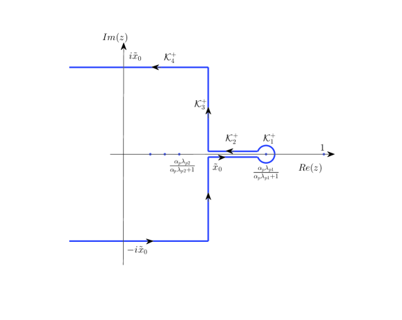
Figure 1: The contour $\mathcal{K}$.

Consider the following integral over the deformed contour $\mathcal{K}$

$$I_{p}(\gamma,\Lambda)=\int_{\mathcal{K}}\left.{}_{1}\mathcal{F}_{0}\left(z\right)\right.\prod_{j=1}^{p}\left(z-\tilde{\lambda}_{pj}\right)^{-\frac{1}{2}}\mathrm{d}z,$$ (37)

where

$$\left.{}_{1}\mathcal{F}_{0}\left(z\right)\right.\equiv\left(1-\frac{h_{p}}{1+h_{p}}z\right)^{\frac{p-n-2}{2}}.$$

For two sequences of random variables $\left\{\xi_{p}\right\}$ and $\left\{\eta_{p}\right\},$ we will write $\xi_{p}\overset{\mathrm{P}}{\sim}\eta_{p}$ if and only if $\xi_{p}/\eta_{p}$ converges in probability to 1 as $p,\mathbf{n}\rightarrow_{\mathbf{c}}\infty$. We have the following lemma.

Lemma 15

Under the hypothesis that $h_{p}=h_{0}$, uniformly in $\gamma$ from any compact subset of $\mathbb{R}$

$$I_{p}(\gamma,\Lambda)\overset{\mathrm{P}}{\sim}\left.{}_{1}\mathcal{F}_{0}\left(\tilde{\lambda}_{p1}\right)\right.2\left(-\frac{\pi}{pH_{0}}\right)^{\frac{1}{2}}\prod_{j=2}^{p}\left(\tilde{\lambda}_{p1}-\tilde{\lambda}_{pj}\right)^{-\frac{1}{2}},$$

where the principal branches of the square roots are used, and

$$H_{0}=\frac{h_{0}(1-c_{2})(\mu_{0}-\sqrt{b_{+}})(\mu_{0}-\sqrt{b_{-}})(c_{1}+c_{2}\mu_{0})}{2c_{1}c_{2}\left(h_{0}-c_{2}\mu_{0}\right)\mu_{0}(c_{1}+h_{0})}$$ (38)

with $\mu_{0}=h_{0}+1$.

Proof: Let $\mathcal{K}_{j}=\mathcal{K}_{j}^{+}\cup\overline{\mathcal{K}_{j}^{+}}$ for $j=1,...,4.$ Using this notation, we can decompose (37) as

$$I_{p}(\gamma,\Lambda)=I_{1,2,p}(\gamma,\Lambda)+I_{3,4,p}(\gamma,\Lambda)$$ (39)

where $I_{1,2,p}(\gamma,\Lambda)$ is the part of the integral corresponding to $\mathcal{K}_{1}\cup\mathcal{K}_{2},$ and $I_{3,4,p}(\theta,\lambda)$ is the part corresponding to the rest of the contour, $\mathcal{K}_{3}\cup\mathcal{K}_{4}$. Our strategy is to show that the integral $I_{p}(\gamma,\Lambda)$ is asymptotically equivalent to $I_{1,2,p}(\gamma,\Lambda)$, the integral $I_{3,4,p}(\gamma,\Lambda)$ being asymptotically dominated by $I_{1,2,p}(\gamma,\Lambda)$.

Let us first focus on $I_{1,2,p}(\gamma,\Lambda)$. Since the singularity of the integrand at $\tilde{\lambda}_{p1}$ is of the inverse square root type, as the radius $\epsilon$ of $\mathcal{K}_{1}$ converges to zero, the integral over $\mathcal{K}_{1}$ converges to zero too. Therefore, we have

$$I_{1,2,p}(\gamma,\Lambda)=2I_{2,p}\left(\gamma,\Lambda\right),$$ (40)

where

$$I_{2,p}\left(\gamma,\Lambda\right)=\int_{\tilde{\lambda}_{p1}}^{\tilde{x}_{0}}\left.{}_{1}\mathcal{F}_{0}\left(z\right)\right.\prod_{j=1}^{p}\left(z-\tilde{\lambda}_{pj}\right)^{-\frac{1}{2}}\mathrm{d}z.$$

Changing the variable of integration from $z$ to $x=\tilde{\lambda}_{p1}-z,$ we arrive at

$$I_{2,p}(\theta,\lambda) =-\int_{0}^{\tilde{\lambda}_{p1}-\tilde{x}_{0}}\left.{}_{1}\mathcal{F}_{0}\left(\tilde{\lambda}_{p1}-x\right)\right.\prod_{j=1}^{p}\left(\tilde{\lambda}_{p1}-\tilde{\lambda}_{pj}-x\right)^{-\frac{1}{2}}\mathrm{d}x$$

$$=\left.{}_{1}\mathcal{F}_{0}\left(\tilde{\lambda}_{p1}\right)\right.(-1)^{\frac{1}{2}}\int_{0}^{\tilde{\lambda}_{p1}-\tilde{x}_{0}}\exp\left\{-pf_{p}(x)\right\}x^{-\frac{1}{2}}\mathrm{d}x$$

where

$$f_{p}(x)=\frac{\beta_{p}}{2}\ln\left(1+\frac{h_{p}(1+\alpha_{p}\lambda_{p1})}{1+h_{p}+\alpha_{p}\lambda_{p1}}x\right)+\frac{1}{2p}\sum_{j=2}^{p}\ln\left(\tilde{\lambda}_{p1}-\tilde{\lambda}_{pj}-x\right)$$

with $\beta_{p}=\left(2+n-p\right)/p$. Now the integral $\int_{0}^{\tilde{\lambda}_{p1}-\tilde{x}_{0}}\exp\left\{-pf_{p}(x)\right\}x^{-\frac{1}{2}}\mathrm{d}x$ can be evaluated using standard Laplace approximation steps (see Olver (1997), section 7.3) as follows.

First, let us show that the derivative $\frac{\mathrm{d}}{\mathrm{d}x}f_{p}(x)$ is continuous and positive on $x\in[0,\tilde{\lambda}_{p1}-\tilde{x}_{0}]$ for sufficiently large $p$ and $\mathbf{n},$ a.s. We have

$$\frac{\mathrm{d}}{\mathrm{d}x}f_{p}(x)=\frac{\beta_{p}}{2}\frac{h_{p}\left(1+\alpha_{p}\lambda_{p1}\right)}{\left(h_{p}+(1+\alpha_{p}\lambda_{p1})(1+h_{p}x)\right)}-\frac{1}{2p}\sum_{j=2}^{p}\left(\tilde{\lambda}_{p1}-\tilde{\lambda}_{pj}-x\right)^{-1}.$$

Therefore, the continuity follows from the fact that, when $h_{p}=h_{0}$,

$$\lambda_{p1}\overset{a.s.}{\rightarrow}x_{1}\equiv\frac{\left(h_{0}+c_{1}\right)\left(h_{0}+1\right)}{h_{0}-\left(h_{0}+1\right)c_{2}}\text{ and }\lambda_{p2}\overset{a.s.}{\rightarrow}b_{+}.$$

In order to establish the positivity, we first obtain

$$\min_{x\in[0,\tilde{\lambda}_{p1}-\tilde{x}_{0}]}\frac{\mathrm{d}}{\mathrm{d}x}f_{p}(x)=\frac{\beta_{p}}{2}\frac{h_{p}}{1+h_{p}-h_{p}\tilde{x}_{0}}-\frac{1}{2p}\sum_{j=2}^{p}\left(\tilde{x}_{0}-\tilde{\lambda}_{pj}\right)^{-1}.$$

It is straightforward to verify that the above equation can be represented in the following form

$$\min_{x\in[0,\tilde{\lambda}_{p1}-\tilde{x}_{0}]}\frac{\mathrm{d}}{\mathrm{d}x}f_{p}(x) =\frac{\beta_{p}}{2}\frac{h_{p}(1+\alpha x_{0})}{1+h_{p}+\alpha x_{0}}+\frac{p-1}{2p}(1+\alpha x_{0})$$

$$+\frac{1}{2\alpha_{p}p}(1+\alpha x_{0})^{2}\sum_{j=2}^{p}\left(\lambda_{pj}-\alpha x_{0}/\alpha_{p}\right)^{-1}.$$

where $x_{0}=\tilde{x}_{0}/\left(\alpha(1-\tilde{x}_{0})\right).$ Therefore, we obtain

$$\min_{x\in[0,\tilde{\lambda}_{p1}-\tilde{x}_{0}]}\frac{\mathrm{d}}{\mathrm{d}x}f_{p}(x)\overset{a.s.}{\rightarrow}\Psi(x_{0},h_{0})$$ (41)

where

$$\Psi(x_{0},h_{0})=\frac{\beta h_{0}(1+\alpha x_{0})}{2(1+h_{0}+\alpha x_{0})}+\frac{1}{2}(1+\alpha x_{0})+\frac{1}{2\alpha}(1+\alpha x_{0})^{2}m\left(x_{0}\right),$$

$$\beta=c_{1}^{-1}+c_{2}^{-1}-1,$$

and $m(x_{0})=\lim_{z\rightarrow x_{0}}m\left(z\right)$ with $m(z)$ being the Stieltjes transform of the limiting spectral distribution of $\mathbf{F},$ that is the distribution with density (10).

Since $m(x_{0})$ is increasing on $x_{0}\in(b_{+},\infty)$, we have

$$\Psi(x_{0},h_{0})>\lim_{x_{0}\downarrow b_{+}}\Psi(x_{0},h_{0}).$$

Moreover, noting the fact that $\lim_{x_{0}\downarrow b_{+}}\Psi(x_{0},h_{0})$ is an increasing function of $h_{0}$ and $h_{0}>\bar{h}\equiv\left(c_{2}+r\right)/\left(1-c_{2}\right)=\sqrt{b_{+}}-1$, we obtain

$$\Psi(x_{0},h_{0})>\lim_{x_{0}\downarrow b_{+}}\Psi(x_{0},h_{0})>\lim_{x_{0}\downarrow b_{+}}\Psi\left(x_{0},\bar{h}\right).$$ (42)

Finally, direct calculations, which are not reported here to save space, show that, as $x_{0}$ converges to $b_{+}$ from the right,

$$m(x_{0})\rightarrow-1/(b_{+}-\sqrt{b_{+}}).$$ (43)

This in turn gives

$$\lim_{x\downarrow b_{+}}\Psi\left(x,\bar{h}\right)=0$$ (44)

which establishes the positivity.

Since $\lambda_{p1}\overset{a.s.}{\rightarrow}x_{1}$, we have

$$f_{p}^{{}^{\prime}}(0)\equiv\left.\frac{\mathrm{d}}{\mathrm{d}x}f_{p}(x)\right|_{x=0}\overset{a.s.}{\rightarrow}H_{0},$$

where

$$H_{0}=\frac{r^{2}}{2c_{1}c_{2}}\frac{(1+\alpha x_{1})h_{0}}{1+h_{0}+\alpha x_{1}}+\frac{1}{2}(1+\alpha x_{1})+\frac{1}{2\alpha}(1+\alpha x_{1})^{2}m(x_{1}).$$

Direct calculations show that

$$m(x_{1})=\lim_{z\rightarrow x_{1}}m(z)=-(1+h_{0})/\left(x_{1}h_{0}\right),$$ (45)

which, after some algebraic manipulations, gives (38).

We may now exploit the approach given in Olver (1997, pp. 81-82) to yield

$$\int_{0}^{\tilde{\lambda}_{p1}-\tilde{x}_{0}}e^{-pf_{p}(x)}x^{-\frac{1}{2}}\mathrm{d}x\overset{\mathrm{P}}{\sim}\left(\frac{\pi}{pf_{p}^{{}^{\prime}}(0)}\right)^{\frac{1}{2}}e^{-pf_{p}(0)}.$$

Therefore, we obtain

$$I_{2,p}(\gamma,\Lambda)\overset{\mathrm{P}}{\sim}\left.{}_{1}\mathcal{F}_{0}\left(\tilde{\lambda}_{p1}\right)\right.\left(-\frac{\pi}{pH_{0}}\right)^{\frac{1}{2}}\prod_{j=2}^{p}\left(\tilde{\lambda}_{p1}-\tilde{\lambda}_{pj}\right)^{-\frac{1}{2}}.$$ (46)

As Lemma 16 below shows, $I_{3,4,p}(\gamma,\Lambda)$ is asymptotically dominated by $I_{2,p}(\theta,\lambda)$, which completes the proof.$\square$

Lemma 16

Under the hypothesis that $h_{p}=h_{0},$ uniformly in $\gamma$ from any compact subset of $\mathbb{R}$

$$I_{3,4,p}(\gamma,\Lambda)=o_{\mathrm{P}}\left(I_{2,p}(\gamma,\Lambda)\right).$$ (47)

Proof: Let us first consider the integral over the contour $\mathcal{K}_{3}$. For $z\in\mathcal{K}_{3}$, we have

$$\left|\left.{}_{1}\mathcal{F}_{0}\left(z\right)\right.\prod_{j=1}^{p}\left(z-\tilde{\lambda}_{pj}\right)^{-\frac{1}{2}}\right|<\left.{}_{1}\mathcal{F}_{0}\left(\tilde{\lambda}_{p1}\right)\right.e^{-pf_{p}\left(\tilde{\lambda}_{p1}-\tilde{x}_{0}\right)}\left(\tilde{\lambda}_{p1}-\tilde{x}_{0}\right)^{-\frac{1}{2}}.$$

Also, in view of (41), (42), and (44), we have $f_{p}(\tilde{\lambda}_{1p}-\tilde{x}_{0})>f_{p}(0)+\epsilon$, for sufficiently large $p$ and $\mathbf{n}$, a.s., where $\epsilon>0$. Therefore, using (46), we conclude

$$\int_{\mathcal{K}_{3}}\left.{}_{1}\mathcal{F}_{0}\left(z\right)\right.\prod_{j=1}^{p}\left(z-\tilde{\lambda}_{pj}\right)^{-\frac{1}{2}}\mathrm{d}z=o_{\mathrm{P}}\left(I_{2,p}(\gamma,\Lambda)\right).$$ (48)

Now consider the integral over the contour $\mathcal{K}_{4}$. We have

$$\left|\int_{\mathcal{K}_{4}}\left.{}_{1}\mathcal{F}_{0}\left(z\right)\right.\prod_{j=1}^{p}\left(z-\tilde{\lambda}_{pj}\right)^{-\frac{1}{2}}\mathrm{d}z\right|<2\prod_{j=1}^{p}\left|\tilde{\lambda}_{pj}-\tilde{x}_{0}\right|^{-\frac{1}{2}}\int_{-\infty}^{\tilde{x}_{0}}\left.{}_{1}\mathcal{F}_{0}\left(x\right)\right.\mathrm{d}x$$

$$\qquad\qquad=4\frac{1+h_{p}}{h_{p}(n-p)}\left(1-\frac{h_{p}}{1+h_{p}}\tilde{x}_{0}\right)\left.{}_{1}\mathcal{F}_{0}\left(\tilde{x}_{0}\right)\right.\prod_{j=1}^{p}\left|\tilde{\lambda}_{pj}-\tilde{x}_{0}\right|^{-\frac{1}{2}}.$$

Since

$$\left.{}_{1}\mathcal{F}_{0}\left(\tilde{x}_{0}\right)\right.\prod_{j=1}^{p}\left(\tilde{\lambda}_{pj}-\tilde{x}_{0}\right)^{-\frac{1}{2}}=\left.{}_{1}\mathcal{F}_{0}\left(\tilde{\lambda}_{p1}\right)\right.e^{-pf_{p}\left(\tilde{\lambda}_{p1}-\tilde{x}_{0}\right)}\left(\tilde{\lambda}_{p1}-\tilde{x}_{0}\right)^{-\frac{1}{2}},$$

we can follow a similar procedure to that outlined above to obtain

$$\int_{\mathcal{K}_{4}}\left.{}_{1}\mathcal{F}_{0}\left(z\right)\right.\prod_{j=1}^{p}\left(z-\tilde{\lambda}_{pj}\right)^{-\frac{1}{2}}\mathrm{d}z=o_{\mathrm{P}}\left(I_{2,p}(\gamma,\Lambda)\right).$$

This along with (48) gives (47).$\square$

5.2 Asymptotic approximation: Setting 2

Consider the following integral

$$J_{p}(\gamma,\Lambda)=\int_{\mathcal{\tilde{K}}}\left.{}_{1}\mathcal{F}_{1}\left(\zeta\right)\right.\prod_{j=1}^{p}\left(z-\tilde{\lambda}_{pj}\right)^{-\frac{1}{2}}\mathrm{d}z,$$

where

$$\left.{}_{1}\mathcal{F}_{1}\left(\zeta\right)\right.\equiv\left.{}_{1}F_{1}\left(n_{A}u+1,n_{A}v+1;n_{A}\zeta\right)\right.$$

with

$$u=\frac{n_{A}+n_{2}-p}{2n_{A}},\text{ }v=\frac{n_{A}-p}{2n_{A}},\text{ and }\zeta=\frac{h_{p}}{2}z.$$

In Johnstone and Onatski (2014) (Theorem 5), the following result is derived. As  $p,\mathbf{n\rightarrow}_{\mathbf{c}}\infty$,

$$\left.{}_{1}\mathcal{F}_{1}\left(\zeta\right)\right.=\frac{C\left(p,\mathbf{n}\right)e^{-n_{A}\varphi\left(\zeta\right)}}{\sqrt{2\pi n_{A}}i}\left(\psi\left(\zeta\right)+O\left(n_{A}^{-1}\right)\right),$$ (49)

where $O\left(n_{A}^{-1}\right)$ is uniform for $\zeta$ that do not approach zero or negative semi-axis and $\mathfrak{R}\left(\zeta\right)\geq-2u+v$,

$$C\left(p,\mathbf{n}\right)=\frac{\Gamma\left(n_{A}v+1\right)\Gamma\left(n_{A}\left(u-v\right)+1\right)}{\Gamma\left(n_{A}u+1\right)},$$

$$\varphi\left(\zeta\right)=\left(u-v\right)\ln\left(u-v\right)+v\ln\left(z_{+}+v\right)-u\ln\left(z_{+}+u\right)-z_{+},$$ (50)

where the principal branches of the logarithms are chosen,

$$z_{+}=\frac{1}{2}\left\{\zeta-v+\sqrt{\left(\zeta-v\right)^{2}+4u\zeta}\right\},$$ (51)

where the principal branch of the square root is chosen when $\mathfrak{R}\left(\zeta\right)\geq-2u+v$ and the other branch is chosen when $\operatorname{Re}\zeta<-2u+v$, and

$$\psi\left(\zeta\right)=\left[\left(z_{+}-\zeta\right)\sqrt{\frac{u}{z_{+}^{2}}-\frac{u-v}{\left(z_{+}-\zeta\right)^{2}}}\right]^{-1},\text{ }$$

where the branch of the square root is chosen so that $\sqrt{-1}=-i.$

We will deform the contour $\mathcal{\tilde{K}}$, without changing the integral’s value with probability approaching one as $p,\mathbf{n}\rightarrow_{\mathbf{c}}\infty$, as shown in Figure 2. Formally, $\mathcal{C}=\mathcal{C}^{+}\cup\overline{\mathcal{C}^{+}}$ with $\mathcal{C}^{+}=\mathcal{C}_{1}^{+}\cup\mathcal{C}_{2}^{+}\cup\mathcal{C}_{3}^{+}\cup\mathcal{C}_{4}^{+}$, where

$$\mathcal{C}_{1}^{+} =\{z:\text{$\Im(z)\geq 0$ and $|z-\tilde{\lambda}_{p1}|=\epsilon\}$},$$

$$\mathcal{C}_{2}^{+} =\{z:z\in[\tilde{x}_{0},\tilde{\lambda}_{p1}-\epsilon]\},$$

$$\mathcal{C}_{3}^{+} =\left\{z:z=2\zeta/h_{p}\text{ s.t. }\mathfrak{R}\left(\zeta\right)\geq-2u+v,\text{ $\Im$}\left(\zeta\right)\geq 0,\text{ }\left|z_{+}+u\right|=\left|z_{0+}+u\right|\right\},$$

$$\mathcal{C}_{4}^{+} =\{z:z=2\zeta/h_{p}\text{ s.t. }\mathfrak{R}\left(\zeta\right)<-2u+v,\text{ and $\Im$}\left(z_{+}\right)=\left|z_{0+}+u\right|\}.$$

Here

$$z_{0+} =\frac{1}{2}\left\{\zeta_{0}-v+\sqrt{\left(\zeta_{0}-v\right)^{2}+4u\zeta_{0}}\right\},\text{ and}$$ (52)

$$\zeta_{0} =\frac{h_{p}}{2}\tilde{x}_{0}.$$

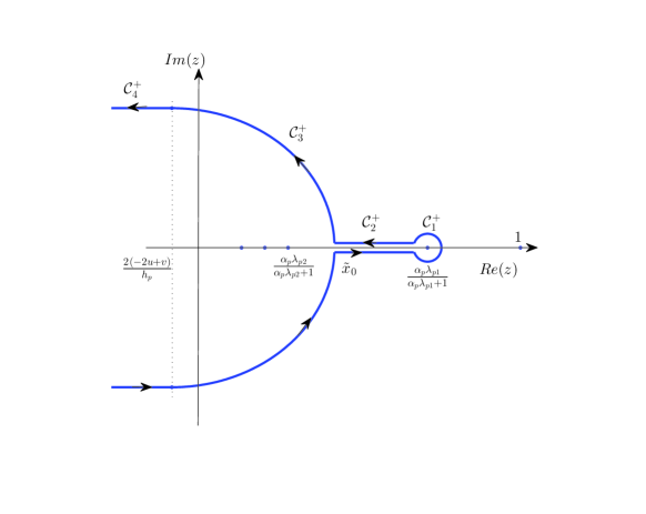
Figure 2: The contour $\mathcal{C}$.

Lemma 17

Under the hypothesis that $h_{p}=h_{0}$, uniformly in $\gamma$ from any compact subset of $\mathbb{R}$

$$J_{p}(\gamma,\Lambda)\overset{\mathrm{P}}{\sim}2Z\left(p,\mathbf{n},h_{0}\right)e^{-n_{A}\varphi\left(\frac{h_{p}}{2}\tilde{\lambda}_{p1}\right)}\left(-\frac{\pi}{pH_{0}}\right)^{1/2}\prod_{j=2}^{p}\left(\tilde{\lambda}_{p1}-\tilde{\lambda}_{pj}\right)^{-\frac{1}{2}},$$

where

$$Z\left(p,\mathbf{n},h_{0}\right)=\frac{C\left(p,\mathbf{n}\right)}{\sqrt{\pi p}}\frac{c_{1}+c_{2}\mu_{0}}{\sqrt{c_{2}\mu_{0}^{2}+c_{1}^{2}-c_{1}+2c_{1}\mu_{0}}},$$

and $H_{0}$ and $\mu_{0}$ are as defined in Lemma 15.

Proof: Similar to the case of Setting 1, we split $J_{p}(\gamma,\Lambda)$ into two parts

$$J_{p}(\gamma,\Lambda)=J_{1,2,p}(\gamma,\Lambda)+J_{3,4,p}(\gamma,\Lambda),$$

where $J_{1,2,p}(\gamma,\Lambda)$ is the part of the integral corresponding to $\mathcal{C}_{1}\cup\mathcal{C}_{2},$ and $J_{3,4,p}(\theta,\lambda)$ is the part corresponding to the rest of the contour, $\mathcal{C}_{3}\cup\mathcal{C}_{4}$. Furthermore,

$$J_{1,2,p}(\gamma,\Lambda)\overset{\mathrm{P}}{\sim}2J_{2,p}\left(\gamma,\Lambda\right),$$ (53)

where

$$J_{2,p}\left(\gamma,\Lambda\right)=\int_{\tilde{\lambda}_{p1}}^{\tilde{x}_{0}}\frac{C\left(p,\mathbf{n}\right)e^{-n_{A}\varphi\left(\zeta\right)}}{\sqrt{2\pi n_{A}}i}\psi\left(\zeta\right)\prod_{j=1}^{p}\left(z-\tilde{\lambda}_{pj}\right)^{-\frac{1}{2}}\mathrm{d}z.$$

In contrast to (40), we only have the asymptotic equivalence in (53) because we are using the uniform asymptotic approximation (49) to define $J_{2,p}\left(\gamma,\Lambda\right).$

After the change of the variable of integration, $\zeta\mapsto x=\frac{h_{p}}{2}\tilde{\lambda}_{p1}-\zeta,$ we obtain

$$J_{2,p}\left(\gamma,\Lambda\right)=-\int_{0}^{\frac{h_{p}}{2}\left(\tilde{\lambda}_{1p}-\tilde{x}_{0}\right)}\frac{C\left(p,\mathbf{n}\right)e^{-n_{A}\varphi\left(\zeta\right)}}{\sqrt{2\pi n_{A}}i}\psi\left(\zeta\right)\frac{2}{h_{p}}\prod_{j=1}^{p}\left(\frac{2}{h_{p}}\zeta-\tilde{\lambda}_{pj}\right)^{-\frac{1}{2}}\mathrm{d}x.$$

This can be rewritten as

$$J_{2,p}\left(\gamma,\Lambda\right)=\left(-\frac{2}{h_{p}}\right)^{\frac{1}{2}}\frac{C\left(p,\mathbf{n}\right)}{\sqrt{2\pi n_{A}}i}\int_{0}^{\frac{h_{p}}{2}\left(\tilde{\lambda}_{p1}-\tilde{x}_{0}\right)}e^{-n_{A}g_{p}(\zeta)}\psi\left(\zeta\right)x^{-\frac{1}{2}}\mathrm{d}x,$$

where

$$g_{p}(\zeta)=\varphi\left(\zeta\right)+\frac{1}{2n_{A}}{\displaystyle\sum\nolimits_{j=2}^{p}}\ln\left(\frac{2}{h_{p}}\zeta-\tilde{\lambda}_{pj}\right),$$

and

$$\zeta=\frac{h_{p}}{2}\tilde{\lambda}_{p1}-x.$$

Following the approach in the above analysis in the case of Setting 1, we now would like to show that the derivative $\frac{\mathrm{d}}{\mathrm{d}x}g_{p}(\frac{h_{p}}{2}\tilde{\lambda}_{p1}-x)$ is continuous and positive on $x\in[0,\frac{h_{p}}{2}\left(\tilde{\lambda}_{p1}-\tilde{x}_{0}\right)]$ for sufficiently large $p$ and $\mathbf{n},$ a.s. This is equivalent to showing that $\frac{\mathrm{d}}{\mathrm{d}\zeta}g_{p}(\zeta)$ is continuous and negative on $\zeta\in[\frac{h_{p}}{2}\tilde{x}_{0},\frac{h_{p}}{2}\tilde{\lambda}_{p1}]$ for sufficiently large $p$ and $\mathbf{n},$ a.s.

It is straightforward to verify that $z_{+}$ satisfies the quadratic equation

$$z_{+}^{2}+(v-\zeta)z_{+}-u\zeta=0,$$

and

$$\zeta=\frac{z_{+}\left(z_{+}+v\right)}{z_{+}+u}.$$ (54)

From this, and the definition (51) of $z_{+},$ we obtain that, $z_{+}>\zeta$ for positive $\zeta,$ and

$$\frac{\mathrm{d}}{\mathrm{d}\zeta}z_{+}=\frac{z_{+}+u}{2z_{+}+v-\zeta}=\frac{\left(u+z_{+}\right)^{2}}{uv+2uz_{+}+z_{+}^{2}}>0.$$ (55)

On the other hand,

$$\frac{\mathrm{d}}{\mathrm{d}z_{+}}\varphi\left(\zeta\right)=\frac{v}{z_{+}+v}-\frac{u}{z_{+}+u}-1=-\frac{uv+2uz_{+}+z_{+}^{2}}{\left(v+z_{+}\right)\left(u+z_{+}\right)}<0$$

Thus, $\varphi\left(\zeta\right)$ is strictly decreasing function of $\zeta.$ Furthermore, it is a convex function of $\zeta>0$. Indeed,

$$\frac{\mathrm{d}^{2}}{\mathrm{d}z_{+}^{2}}\varphi\left(\zeta\right)=-\frac{v}{\left(z_{+}+v\right)^{2}}+\frac{u}{\left(z_{+}+u\right)^{2}}=\frac{\left(u-v\right)\left(z_{+}^{2}-uv\right)}{\left(z_{+}+v\right)^{2}\left(z_{+}+u\right)^{2}},$$

and, using (54) and (55), we also have

$$\frac{\mathrm{d}^{2}}{\mathrm{d}\zeta^{2}}z_{+}=-2u\left(u+z_{+}\right)^{3}\frac{u-v}{\left(uv+2uz_{+}+z_{+}^{2}\right)^{3}}.$$

Therefore, we obtain

$$\frac{\mathrm{d}^{2}}{\mathrm{d}\zeta^{2}}\varphi\left(\zeta\right) =\frac{\mathrm{d}^{2}}{\mathrm{d}z_{+}^{2}}\varphi\left(\zeta\right)\left(\frac{\mathrm{d}}{\mathrm{d}\zeta}z_{+}\right)^{2}+\frac{\mathrm{d}}{\mathrm{d}z_{+}}\varphi\left(\zeta\right)\frac{\mathrm{d}^{2}}{\mathrm{d}\zeta^{2}}z_{+}$$

$$=\frac{\left(u+z_{+}\right)^{2}\left(u-v\right)}{\left(v+z_{+}\right)^{2}\left(uv+2uz_{+}+z_{+}^{2}\right)}>0.$$

Therefore, $\varphi\left(\zeta\right)$ is, indeed, convex for positive $\zeta,$ and has a continuous derivative.

Further, it is straightforward to see that

$$w\left(\zeta\right)\equiv\frac{1}{2n_{A}}{\displaystyle\sum\nolimits_{j=2}^{p}}\ln\left(\frac{2}{h_{p}}\zeta-\tilde{\lambda}_{pj}\right)$$

is a strictly increasing concave function of $\zeta>\frac{h_{p}}{2}\tilde{\lambda}_{p2}$. This implies that

$$\max_{\zeta\in\left[\frac{h_{p}}{2}\tilde{x}_{0},\frac{h_{p}}{2}\tilde{\lambda}_{p1}\right]}\frac{\mathrm{d}}{\mathrm{d}\zeta}g_{p}\left(\zeta\right) <\left.\frac{\mathrm{d}}{\mathrm{d}\zeta}\varphi\left(\zeta\right)\right|_{\zeta=\frac{h_{p}}{2}\tilde{\lambda}_{1p}}+\left.\frac{\mathrm{d}}{\mathrm{d}\zeta}w\left(\zeta\right)\right|_{\zeta=\frac{h_{p}}{2}\tilde{x}_{0}}$$

$$=\left.-\frac{uv+2uz_{+}+z_{+}^{2}}{\left(v+z_{+}\right)\left(u+z_{+}\right)}\left(1+\frac{u(u-v)}{2z_{+}\left(u+z_{+}\right)}\right)\right|_{\zeta=\frac{h_{p}}{2}\tilde{\lambda}_{1p}}$$

$$-\frac{2p}{h_{p}n_{A}}\frac{p-1}{2p}(1+\alpha x_{0})$$

$$-\frac{2p}{h_{p}n_{A}}\frac{1}{2\alpha_{p}p}(1+\alpha x_{0})^{2}\sum_{j=2}^{p}\left(\lambda_{j}-\alpha x_{0}/\alpha_{p}\right)^{-1}$$

The right hand side of the latter equality a.s. converges to

$$\Pi(x_{0},h_{0})=-\frac{c_{1}}{c_{2}\left(h_{0}+1\right)}-1-\frac{c_{1}}{h_{0}}(1+\alpha x_{0})-\frac{c_{1}}{h_{0}\alpha}(1+\alpha x_{0})^{2}m\left(x_{0}\right),$$

where $m(z)$ is the Stieltjes transform of the limiting spectral distribution of $\mathbf{F}.$ Since $m(x_{0})$ is an increasing function of $x_{0}>b_{+}$,

$$\Pi(x_{0},h_{0})<\lim_{x_{0}\downarrow b_{+}}\Pi(x_{0},h_{0}).$$

On the other hand, using (43), we get

$$\lim_{x_{0}\downarrow b_{+}}\Pi(x_{0},h_{0})=-\frac{c_{1}}{c_{2}\left(h_{0}+1\right)}-1+r\frac{\left(r+c_{2}\right)^{2}}{c_{2}h_{0}\left(1-c_{2}\right)\left(r+1\right)}.$$ (56)

Note that, considered as a function of $h_{0}>\bar{h},$ $\lim_{x_{0}\downarrow b_{+}}\Pi(x_{0},h_{0})$ may have positive derivative only when $\lim_{x_{0}\downarrow b_{+}}\Pi(x_{0},h_{0})<0.$ Indeed,

$$\frac{\mathrm{d}}{\mathrm{d}h_{0}}\lim_{x_{0}\downarrow b_{+}}\Pi(x_{0},h_{0}) =\frac{c_{1}}{c_{2}\left(h_{0}+1\right)^{2}}-r\frac{\left(r+c_{2}\right)^{2}}{c_{2}h_{0}^{2}\left(1-c_{2}\right)\left(r+1\right)}$$

$$<\frac{1}{h_{0}}\left(\frac{c_{1}}{c_{2}\left(h_{0}+1\right)}-r\frac{\left(r+c_{2}\right)^{2}}{c_{2}h_{0}\left(1-c_{2}\right)\left(r+1\right)}\right)$$

If the latter expression is positive for $h_{0}>\bar{h}>0$, then $\lim_{x_{0}\downarrow b_{+}}\Pi(x_{0},h_{0})$ is clearly negative. Therefore,

$$\lim_{x_{0}\downarrow b_{+}}\Pi(x_{0},h_{0})<\max\left\{0,\lim_{x_{0}\downarrow b_{+}}\Pi(x_{0},\bar{h})\right\}.$$

But, using the definition $\bar{h}=\left(c_{2}+r\right)/\left(1-c_{2}\right)$ in (56), we obtain

$$\lim_{x_{0}\downarrow b_{+}}\Pi(x_{0},\bar{h})=-\frac{c_{1}\left(1-c_{2}\right)}{c_{2}\left(1+r\right)}-1+r\frac{\left(r+c_{2}\right)}{c_{2}\left(r+1\right)}=0.$$

This implies that $\max_{\zeta\in\left[\frac{h_{p}}{2}\tilde{x}_{0},\frac{h_{p}}{2}\tilde{\lambda}_{1p}\right]}\frac{\mathrm{d}}{\mathrm{d}\zeta}g_{p}\left(\zeta\right)$ is a.s. negative for sufficiently large $p$ and $\mathbf{n}$.

Now, since $\lambda_{p1}\overset{a.s.}{\rightarrow}x_{1}$, we have

$$g_{p}^{{}^{\prime}}(0)\equiv\left.-\frac{\mathrm{d}}{\mathrm{d}\zeta}g_{p}(\zeta)\right|_{\zeta=\frac{h_{p}}{2}\tilde{\lambda}_{p1}}\overset{a.s.}{\rightarrow}R_{0},$$

where

$$R_{0}=\frac{c_{1}}{c_{2}\left(h_{0}+1\right)}+1+\frac{c_{1}}{h_{0}}(1+\alpha x_{1})+\frac{c_{1}}{\alpha h_{0}}(1+\alpha x_{1})^{2}m(x_{1}).$$

Using (45), (36) and (38), we obtain

$$R_{0}=2c_{1}H_{0}/h_{0}.$$

Exploiting the approach given in Olver (1997, pp. 81-82), we obtain

$$\int_{0}^{\frac{h_{p}}{2}\left(\tilde{\lambda}_{p1}-\tilde{x}_{0}\right)}e^{-n_{A}g_{p}(\zeta)}\psi\left(\zeta\right)x^{-\frac{1}{2}}\mathrm{d}x\overset{\mathrm{P}}{\sim}\left(\frac{\pi}{n_{A}g_{p}^{{}^{\prime}}(0)}\right)^{\frac{1}{2}}e^{-n_{A}g_{p}\left(\frac{h_{p}}{2}\tilde{\lambda}_{p1}\right)}\psi\left(\frac{h_{0}\alpha x_{1}}{2\left(1+\alpha x_{1}\right)}\right).$$

On the other hand, direct calculation shows that

$$\psi\left(\frac{h_{0}\alpha x_{1}}{2\left(1+\alpha x_{1}\right)}\right)=i\frac{\sqrt{2}\left(c_{1}+c_{2}+c_{2}h_{0}\right)}{\sqrt{c_{1}}\sqrt{c_{2}\mu_{0}^{2}+c_{1}^{2}-c_{1}+2c_{1}\mu_{0}}},$$

and

$$g_{p}\left(\frac{h_{p}}{2}\tilde{\lambda}_{p1}\right)=\varphi\left(\frac{h_{p}}{2}\tilde{\lambda}_{p1}\right)+\frac{1}{2n_{A}}{\displaystyle\sum\nolimits_{j=2}^{p}}\ln\left(\tilde{\lambda}_{p1}-\tilde{\lambda}_{pj}\right).$$

Therefore,

$$J_{2,p}(\gamma,\Lambda)\overset{\mathrm{P}}{\sim}Z\left(p,\mathbf{n},h_{0}\right)\left(-\frac{\pi}{pH_{0}}\right)^{\frac{1}{2}}e^{-n_{A}\varphi\left(\frac{h_{p}}{2}\tilde{\lambda}_{p1}\right)}\prod_{j=2}^{p}\left(\tilde{\lambda}_{p1}-\tilde{\lambda}_{pj}\right)^{-\frac{1}{2}},$$ (57)

where

$$Z\left(p,\mathbf{n},h_{0}\right)=\frac{C\left(p,\mathbf{n}\right)}{\sqrt{\pi p}}\frac{c_{1}+c_{2}\mu_{0}}{\sqrt{c_{2}\mu_{0}^{2}+c_{1}^{2}-c_{1}+2c_{1}\mu_{0}}}.$$

As Lemma 18 below shows, $J_{3,4,p}(\gamma,\Lambda)$ is asymptotically dominated by $J_{2,p}(\theta,\lambda)$, which completes the proof.$\square$

Lemma 18

Under the hypothesis that $h_{p}=h_{0},$ uniformly in $\gamma$ from any compact subset of $\mathbb{R}$

$$J_{3,4,p}(\gamma,\Lambda)=o_{\mathrm{P}}\left(J_{2,p}(\gamma,\Lambda)\right).$$

Proof: Let us first consider the integral $J_{3,p}(\gamma,\Lambda)$ over the contour $\mathcal{C}_{3}$. For $z\in\mathcal{C}_{3}$, by definition, we have $\mathfrak{R}\left(\zeta\right)\equiv\mathfrak{R}\left(h_{p}z/2\right)\geq-2u+v$. Therefore, the uniform approximation (49) is still valid, and we have

$$J_{3,p}\left(\gamma,\Lambda\right)\overset{\mathrm{P}}{\sim} \int_{\mathcal{C}_{3}}\frac{C\left(p,\mathbf{n}\right)e^{-n_{A}\varphi\left(\zeta\right)}}{\sqrt{2\pi n_{A}}i}\psi\left(\zeta\right)\prod_{j=1}^{p}\left(z-\tilde{\lambda}_{pj}\right)^{-\frac{1}{2}}\mathrm{d}z$$ (58)

$$=\int_{\mathcal{C}_{3}}\frac{C\left(p,\mathbf{n}\right)e^{-n_{A}g_{p}\left(\zeta\right)}}{\sqrt{2\pi n_{A}}i}\psi\left(\zeta\right)\left(z-\tilde{\lambda}_{p1}\right)^{-\frac{1}{2}}\mathrm{d}z.$$

Let us show that, for $\zeta=h_{p}z/2$ with $z\in\mathcal{C}_{3},$

$$\mathfrak{R}g_{p}\left(\zeta\right)>g_{p}\left(h_{p}\tilde{x}_{0}/2\right).$$ (59)

Recall that

$$g_{p}(\zeta) =\varphi\left(\zeta\right)+\frac{1}{2n_{A}}{\displaystyle\sum\nolimits_{j=2}^{p}}\ln\left(\frac{2}{h_{p}}\zeta-\tilde{\lambda}_{pj}\right),\text{ and}$$

$$\varphi\left(\zeta\right) =\left(u-v\right)\ln\left(u-v\right)+v\ln\left(z_{+}+v\right)-u\ln\left(z_{+}+u\right)-z_{+}.$$

By definition of $\mathcal{C}_{3},$ as $z$ moves along $\mathcal{C}_{3}$ away from $\tilde{x}_{0},$ $\zeta$ is changing so that $z_{+}$ moves along a circle with center at $-u$ and radius $z_{0+}+u,$ where $z_{0+}$ is as defined in (52). In particular, $\left|z_{+}+u\right|$ remains constant, $\mathfrak{R}\left(-z_{+}\right)$ increases, and, since $v<u,$ $\left|z_{+}+v\right|$ increases too. Overall,

$$\mathfrak{R}\left(\varphi\left(\zeta\right)\right)=\left(u-v\right)\ln\left(u-v\right)+v\ln\left|z_{+}+v\right|-u\ln\left|z_{+}+u\right|+\mathfrak{R}\left(-z_{+}\right)$$

is increasing. Note also that $\left|\zeta\right|=\left|z_{+}\right|\left|z_{+}+v\right|/\left|z_{+}+u\right|$ must increase, which implies that $\left|\frac{2}{h_{p}}\zeta-\tilde{\lambda}_{pj}\right|$ is increasing for all $j\geq 2,$ and thus,

$$\mathfrak{R}\left(\frac{1}{2n_{A}}{\displaystyle\sum\nolimits_{j=2}^{p}}\ln\left(\frac{2}{h_{p}}\zeta-\tilde{\lambda}_{pj}\right)\right)$$

is increasing too. This implies (59).

On the other hand, in the above proof of Lemma 17 we have shown that $\frac{\mathrm{d}}{\mathrm{d}\zeta}g_{p}(\zeta)$ is continuous and negative on $\zeta\in[\frac{h_{p}}{2}\tilde{x}_{0},\frac{h_{p}}{2}\tilde{\lambda}_{p1}].$ Hence, there must exist $C>0$ such that, for any $\zeta=h_{p}z/2$ with $z\in\mathcal{C}_{3},$

$$\left|e^{-n_{A}g_{p}\left(\zeta\right)}\right|\leq e^{-n_{A}C}e^{-n_{A}\varphi\left(\frac{h_{p}}{2}\tilde{\lambda}_{p1}\right)}\prod_{j=2}^{p}\left(\tilde{\lambda}_{p1}-\tilde{\lambda}_{pj}\right)^{-\frac{1}{2}}.$$

This inequality, together with (57) and (58) imply that

$$J_{3,p}\left(\gamma,\Lambda\right)=o_{\mathrm{P}}\left(J_{2,p}(\gamma,\Lambda)\right).$$

The fact that $J_{4,p}\left(\gamma,\Lambda\right)=o_{\mathrm{P}}\left(J_{2,p}(\gamma,\Lambda)\right)$ follows from pp. 29-31 of Johnstone and Onatski (2014).$\square$

6 Local Asymptotic Normality

6.1 Analysis for Setting 1

Let us denote the likelihood ratio by

$$L_{p1}(\gamma,\Lambda)=\frac{f_{1}(\Lambda;h_{p})}{f_{1}(\Lambda;h_{0})}.$$ (60)

From Lemmas 14 and 15, we obtain the following expression

$$f_{1}(\Lambda;h_{p})=\frac{1}{2\pi i}C_{p1}(\Lambda)k_{p1}(h_{p})I_{p}(\gamma,\Lambda).$$

Using Lemma 15, we obtain

$$L_{p1}(\gamma,\Lambda)\overset{\mathrm{P}}{\sim}\frac{k_{p1}(h_{p})}{k_{p1}(h_{0})}\left(\frac{1-\frac{h_{p}}{1+h_{p}}\tilde{\lambda}_{p1}}{1-\frac{h_{0}}{1+h_{0}}\tilde{\lambda}_{p1}}\right)^{\frac{p-n-2}{2}}.$$ (61)

Consider a new local parameter

$$\theta_{1}=\gamma/\omega_{1}\left(h_{0}\right),$$

where

$$\omega_{1}\left(h_{0}\right)=\frac{2h_{0}^{2}\left(1+h_{0}\right)^{2}r^{2}}{\left(h_{0}-c_{2}\left(1+h_{0}\right)\right)^{2}}.$$

We have the following lemma.

Lemma 19

Let Under the null hypothesis that $h=h_{0}$, uniformly in $\theta_{1}$ from any compact subset of $\mathbb{R}$,

$$\ln L_{p1}(\gamma,\Lambda)=\theta_{1}\sqrt{p}\left(\lambda_{p1}-x_{p1}\right)-\frac{1}{2}\theta_{1}^{2}\tau_{1}^{2}(h_{0})+o_{\mathrm{P}}(1)$$

where

$$x_{p1} =\frac{\left(h_{0}+p/n_{1}\right)\left(h_{0}+1\right)}{h_{0}-\left(h_{0}+1\right)p/n_{2}},\text{ and}$$

$$\tau_{1}^{2}(h_{0}) =2r^{2}\frac{h_{0}^{2}\left(h_{0}+1\right)^{2}\left(h_{0}^{2}-c_{2}\left(h_{0}+1\right)^{2}-c_{1}\right)}{\left(c_{2}-h_{0}+c_{2}h_{0}\right)^{4}}.$$

Proof: Taking the logarithm of (61) yields

$$\ln L_{p1}(\gamma,\Lambda) =\frac{n+2-p}{2}\left(\ln\left(1-\frac{\tilde{\lambda}_{p1}h_{0}}{1+h_{0}}\right)-\ln\left(1-\frac{\tilde{\lambda}_{p1}h_{p}}{1+h_{p}}\right)\right)$$

$$-\left(\frac{p-2}{2}\right)\ln\frac{h_{p}}{h_{0}}+\left(\frac{p-n_{1}-2}{2}\right)\ln\frac{1+h_{p}}{1+h_{0}}+o_{\mathrm{P}}(1).$$ (62)

Moreover, we have the following expansions

$$\ln\left(1-\frac{\tilde{\lambda}_{p1}h_{0}}{1+h_{0}}\right)-\ln\left(1-\frac{\tilde{\lambda}_{p1}h_{p}}{1+h_{p}}\right) =p^{-\frac{1}{2}}\gamma\frac{\tilde{\lambda}_{p1}}{(1+h_{0})\left(1+h_{0}(1-\tilde{\lambda}_{p1})\right)}$$

$$-p^{-1}\gamma^{2}\frac{\tilde{\lambda}_{p1}}{(1+h_{0})^{2}(1+h_{0}(1-\tilde{\lambda}_{p1}))}$$ (63)

$$\quad+p^{-1}\gamma^{2}\frac{{\tilde{\lambda}_{p1}}^{2}}{2(1+h_{0})^{2}(1+h_{0}(1-\tilde{\lambda}_{p1}))^{2}}+o_{\mathrm{P}}(p^{-1}),$$

$$\ln\frac{1+h_{p}}{1+h_{0}}=p^{-\frac{1}{2}}\gamma\frac{1}{1+h_{0}}-p^{-1}\gamma^{2}\frac{1}{2(1+h_{0})^{2}}+o(p^{-1}),$$ (64)

and

$$\ln\frac{h_{p}}{h_{0}}=p^{-\frac{1}{2}}\gamma h_{0}^{-1}-\frac{1}{2}p^{-1}\gamma^{2}h_{0}^{-2}+o(p^{-1}).$$ (65)

Finally, using (63), (64), and (65) in (62) and noting the fact that $\lambda_{1}-x_{p1}\overset{a.s.}{\rightarrow}0,$ we obtain the statement of the lemma by straightforward algebraic manipulations.$\square$

Lemma 19 together with the asymptotic normality of $\sqrt{p}\left(\lambda_{p1}-x_{p1}\right)$ established in Proposition 11 imply, via Le Cam’s First Lemma (see van der Vaart (1998), p.88), that the sequences of the probability measures $\left\{\mathbb{P}_{h_{0},p}\right\}$ and $\left\{\mathbb{P}_{h_{0}+\gamma/\sqrt{p},p}\right\}$ describing the joint distribution of the eigenvalues of $\mathbf{F}$ under the null $H_{0}:h_{p}=h_{0}$ and under the local alternative $H_{1}:h_{p}=h_{0}+\gamma/\sqrt{p}$ are mutually contiguous. Moreover, the experiments $\left(\mathbb{P}_{h_{0}+\theta_{1}\omega_{1}\left(h_{0}\right)/\sqrt{p},p}:\theta_{1}\in\mathbb{R}\right)$ converge to the Gaussian shift experiment $\left(N\left(\theta_{1},\tau_{1}^{2}(h_{0})\right):\theta_{1}\in\mathbb{R}\right)$. In particular, these experiments are LAN.

6.2 Analysis for Setting 2

Let us denote the likelihood ratio by

$$L_{p2}(\gamma,\Lambda)=\frac{f_{2}(\Lambda;h_{p})}{f_{2}(\Lambda;h_{0})}.$$ (66)

From Lemmas 14 and 17, we obtain the following expression

$$f_{2}(\Lambda;h_{p})=\frac{1}{2\pi i}C_{p2}(\Lambda)k_{p2}(h_{p})J_{p}(\gamma,\Lambda).$$

Using Lemma 17, and the definitions (50) and (51), we obtain

$$L_{p2}(\gamma,\Lambda)\overset{\mathrm{P}}{\sim}\exp\left[-n_{A}{\displaystyle\sum\nolimits_{j=1}^{4}}\left(a_{j}\left(h_{p}\right)-a_{j}\left(h_{0}\right)\right)\right],$$ (67)

where

$$a_{1}\left(h\right)=\frac{h+\ln h}{2},$$

$$a_{2}(h)=-\frac{1}{2}\left(\frac{h}{2}\tilde{\lambda}_{p1}-v+\sqrt{\left(\frac{h}{2}\tilde{\lambda}_{p1}-v\right)^{2}+4u\frac{h}{2}\tilde{\lambda}_{p1}}\right),$$

$$a_{3}(h)=-u\ln\left[\frac{1}{2}\left(\frac{h}{2}\tilde{\lambda}_{p1}-v+\sqrt{\left(\frac{h}{2}\tilde{\lambda}_{p1}-v\right)^{2}+4u\frac{h}{2}\tilde{\lambda}_{p1}}\right)\right],$$

and

$$a_{4}\left(h\right)=\left(u-v\right)\ln\left[\frac{1}{2}\left(-\frac{h}{2}\tilde{\lambda}_{p1}-v+\sqrt{\left(\frac{h}{2}\tilde{\lambda}_{p1}-v\right)^{2}+4u\frac{h}{2}\tilde{\lambda}_{p1}}\right)\right].$$

We would like, first, to expand $a_{j}\left(h_{p}\right)-a_{j}(h_{0}),$ with $j=1,...,4,$ in the power series of $\gamma/\sqrt{p}$ up to, and including, the terms of order $O_{\mathrm{P}}\left(\frac{1}{p}\right).$ For $a_{1},$ we have

$$a_{1}\left(h_{p}\right)-a_{1}(h_{0})=\frac{h_{0}+1}{2h_{0}}\frac{\gamma}{\sqrt{p}}-\frac{1}{4h_{0}^{2}}\frac{\gamma^{2}}{p}.$$ (68)

For $a_{2},$ note that

$$\left(\frac{h_{p}}{2}\tilde{\lambda}_{p1}-v\right)^{2}+4u\frac{h_{p}}{2}\tilde{\lambda}_{p1} =\left(\frac{h_{0}}{2}\tilde{\lambda}_{p1}-v\right)^{2}+4u\frac{h_{0}}{2}\tilde{\lambda}_{p1}$$

$$+\left(\frac{h_{0}}{2}\tilde{\lambda}_{p1}+2u-v\right)\frac{\gamma}{\sqrt{p}}\tilde{\lambda}_{p1}+\frac{\gamma^{2}}{4p}\tilde{\lambda}_{p1}^{2}.$$

Using this expression and the facts that, when $h_{p}=h_{0},$

$$\tilde{\lambda}_{p1}\overset{a.s.}{\rightarrow}\frac{\left(h_{0}+1\right)\left(c_{1}+h_{0}\right)}{h_{0}\left(1+c_{1}/c_{2}+h_{0}\right)},\text{ }u\rightarrow\frac{1+c_{1}/c_{2}-c_{1}}{2},\text{ and }v\rightarrow\frac{1-c_{1}}{2},$$

we obtain after some algebra,

$$a_{2}\left(h_{p}\right)-a_{2}(h_{0})=-\frac{\tilde{\lambda}_{1p}}{4}\left(1+\frac{\frac{h_{0}}{2}\tilde{\lambda}_{p1}+2u-v}{S}\right)\frac{\gamma}{\sqrt{p}}+C^{(2)}\frac{\gamma^{2}}{p}+o_{\mathrm{P}}\left(\frac{1}{p}\right),$$ (69)

where

$$S=\sqrt{\left(\frac{h_{0}}{2}\tilde{\lambda}_{p1}-v\right)^{2}+4u\frac{h_{0}}{2}\tilde{\lambda}_{p1}},$$

and

$$C^{(2)}=\frac{c_{1}\left(h_{0}+1\right)^{2}\left(c_{1}+h_{0}\right)^{2}\left(c_{1}+c_{2}-c_{1}c_{2}\right)\left(c_{2}+c_{1}+h_{0}c_{2}\right)}{2h_{0}^{2}\left(2c_{2}h_{0}+c_{1}^{2}+c_{2}+c_{2}h_{0}^{2}+c_{1}+2h_{0}c_{1}\right)^{3}}.$$

For $a_{3},$ we have

$$a_{3}\left(h_{p}\right)-a_{3}(h_{0}) =-\frac{u\tilde{\lambda}_{p1}\left(\frac{h_{0}}{2}\tilde{\lambda}_{p1}+2u-v+S\right)}{2\left(\left(\frac{h_{0}}{2}\tilde{\lambda}_{p1}-v\right)^{2}+4u\frac{h_{0}}{2}\tilde{\lambda}_{p1}+\left(\frac{h_{0}}{2}\tilde{\lambda}_{p1}-v\right)S\right)}\frac{\gamma}{\sqrt{p}}$$ (70)

$$+C^{(2)}C^{(3)}\frac{\gamma^{2}}{p}+o_{\mathrm{P}}\left(\frac{1}{p}\right),$$

where

$$C^{(3)}=\frac{\left(c_{1}+c_{2}-c_{1}c_{2}\right)}{c_{2}\left(c_{1}+h_{0}\right)}+\frac{\left(2c_{2}h_{0}+c_{1}^{2}+c_{2}+c_{2}h_{0}^{2}+c_{1}+2h_{0}c_{1}\right)\left(c_{1}+c_{2}+c_{2}h_{0}\right)}{2c_{1}c_{2}\left(c_{1}+h_{0}\right)^{2}}.$$

Finally, for $a_{4},$ we obtain

$$a_{4}\left(h_{p}\right)-a_{4}(h_{0}) =\frac{\left(u-v\right)\tilde{\lambda}_{p1}\left(\frac{h_{0}}{2}\tilde{\lambda}_{p1}+2u-v-S\right)}{2\left(\left(\frac{h_{0}}{2}\tilde{\lambda}_{p1}-v\right)^{2}+4u\frac{h_{0}}{2}\tilde{\lambda}_{p1}+\left(-\frac{h_{0}}{2}\tilde{\lambda}_{p1}-v\right)S\right)}\frac{\gamma}{\sqrt{p}}$$ (71)

$$-C^{(2)}C^{(4)}\frac{\gamma^{2}}{p}+o_{\mathrm{P}}\left(\frac{1}{p}\right),$$

where

$$C^{(4)}=\frac{c_{1}+c_{2}+c_{2}h_{0}}{c_{2}\left(c_{1}+h_{0}\right)}+\frac{\left(c_{1}+c_{2}-c_{1}c_{2}\right)\left(c_{1}+c_{2}+c_{2}h_{0}^{2}+c_{1}^{2}+2c_{1}h_{0}+2c_{2}h_{0}\right)}{2c_{2}\left(c_{1}+h_{0}\right)^{2}\left(c_{1}+c_{2}+c_{2}h_{0}\right)}.$$

Summing up the $\gamma^{2}/p$ terms in the expansions (68-71), we obtain that the $\gamma^{2}/p$ term in the expansion of ${\displaystyle\sum\nolimits_{j=1}^{4}}\left(a_{j}\left(h_{p}\right)-a_{j}\left(h_{0}\right)\right)$, which we will refer as $T_{2}$, equals

$$T_{2}=-\frac{1}{4}c_{1}\frac{c_{1}+c_{2}+c_{2}h_{0}^{2}-h_{0}^{2}+2c_{2}h_{0}}{h_{0}^{2}\left(c_{1}+c_{2}+c_{2}h_{0}^{2}+c_{1}^{2}+2c_{1}h_{0}+2c_{2}h_{0}\right)}\frac{\gamma^{2}}{p}.$$ (72)

Now let $\Delta=\sqrt{p}\left(\lambda_{p1}-x_{p1}\right),$ where

$$x_{p1}=\frac{\left(h_{0}+p/n_{1}\right)\left(h_{0}+1\right)}{h_{0}-\left(h_{0}+1\right)p/n_{2}},$$

so that

$$\tilde{\lambda}_{p1} =\frac{\lambda_{p1}}{\frac{n_{2}}{n_{1}}+\lambda_{p1}}=\frac{x_{p1}+\Delta/\sqrt{p}}{\frac{n_{2}}{n_{1}}+x_{p1}+\Delta/\sqrt{p}}$$

$$=\frac{\left(h_{0}+1\right)\left(p/n_{1}+h_{0}\right)}{h_{0}\left(1+n_{2}/n_{1}+h_{0}\right)}+\frac{\Delta}{\sqrt{p}}\frac{c_{2}c_{1}\left(c_{2}+c_{2}h_{0}-h_{0}\right)^{2}}{h_{0}^{2}\left(c_{2}+c_{1}+c_{2}h_{0}\right)^{2}}+o_{\mathrm{P}}\left(\frac{1}{\sqrt{p}}\right),$$

Our next goal is to expand the weights on $\gamma/\sqrt{p}$ in expansions (68-71) into power series of $\Delta/\sqrt{p}$ up to the linear term only.

For (69), we have

$$-\frac{\tilde{\lambda}_{p1}}{4}\left(1+\frac{\frac{h_{0}}{2}\tilde{\lambda}_{p1}+2u-v}{S}\right)=\tau_{0}^{(2)}+\left[\tau_{11}^{(2)}+\tau_{12}^{(2)}\right]\frac{\Delta}{\sqrt{p}}+o_{\mathrm{P}}\left(\frac{1}{\sqrt{p}}\right),$$

where

$$\tau_{11}^{(2)}=-\frac{c_{1}\left(c_{2}+c_{2}h_{0}-h_{0}\right)^{2}}{2h_{0}^{2}\left(c_{1}+c_{2}+c_{2}h_{0}^{2}+c_{1}^{2}+2c_{1}h_{0}+2c_{2}h_{0}\right)},$$

$$\tau_{12}^{(2)}=\frac{c_{1}^{2}\left(h_{0}+1\right)\left(c_{1}+h_{0}\right)\left(c_{1}+c_{2}-c_{1}c_{2}\right)\left(c_{2}+c_{2}h_{0}-h_{0}\right)^{2}}{h_{0}^{2}\left(c_{1}+c_{2}+c_{2}h_{0}^{2}+c_{1}^{2}+2c_{1}h_{0}+2c_{2}h_{0}\right)^{3}},$$

and $\tau_{0}^{(2)}$ is a complicated function of $h_{0},p,n_{1},$ and $n_{2}$, which we do not report here.

For (70), we have

$$-\frac{u\tilde{\lambda}_{p1}\left(\frac{h_{0}}{2}\tilde{\lambda}_{p1}+2u-v+S\right)}{2\left(\left(\frac{h_{0}}{2}\tilde{\lambda}_{p1}-v\right)^{2}+4u\frac{h_{0}}{2}\tilde{\lambda}_{p1}+\left(\frac{h_{0}}{2}\tilde{\lambda}_{p1}-v\right)S\right)}=\tau_{0}^{(3)}+\left[\tau_{11}^{(3)}+\tau_{12}^{(3)}\right]\frac{\Delta}{\sqrt{p}}+o_{\mathrm{P}}\left(\frac{1}{\sqrt{p}}\right),$$

where

$$\tau_{11}^{(3)}=\frac{c_{1}\left(c_{2}-h_{0}+c_{2}h_{0}\right)^{2}\left(c_{1}+c_{2}-c_{1}c_{2}\right)\left(c_{1}+c_{2}+c_{2}h_{0}\right)\left(c_{1}+c_{2}+c_{2}h_{0}^{2}-c_{1}^{2}+2c_{2}h_{0}\right)}{2h_{0}^{2}c_{2}\left(c_{1}+c_{2}+c_{2}h_{0}^{2}+c_{1}^{2}+2c_{1}h_{0}+2c_{2}h_{0}\right)^{3}},$$

$$\tau_{12}^{(3)}=-\frac{c_{1}\left(h_{0}+1\right)\left(c_{2}-h_{0}+c_{2}h_{0}\right)^{2}\left(c_{1}+c_{2}-c_{1}c_{2}\right)}{2h_{0}^{2}\left(c_{1}+c_{2}+c_{2}h_{0}^{2}+c_{1}^{2}+2c_{1}h_{0}+2c_{2}h_{0}\right)^{2}},$$

and $\tau_{0}^{(3)}$ is a complicated function of $h_{0},p,n_{1},$ and $n_{2}$, which we do not report here.

For (71), we have

$$\frac{\left(u-v\right)\tilde{\lambda}_{p1}\left(\frac{h_{0}}{2}\tilde{\lambda}_{p1}+2u-v-S\right)}{2\left(\left(\frac{h_{0}}{2}\tilde{\lambda}_{p1}-v\right)^{2}+4u\frac{h_{0}}{2}\tilde{\lambda}_{p1}+\left(-\frac{h_{0}}{2}\tilde{\lambda}_{p1}-v\right)S\right)}=\tau_{0}^{(4)}+\left[\tau_{11}^{(4)}+\tau_{12}^{(4)}\right]\frac{\Delta}{\sqrt{p}}+o_{\mathrm{P}}\left(\frac{1}{\sqrt{p}}\right),$$

where

$$\tau_{11}^{(4)}=\frac{c_{1}^{3}\left(c_{2}-h_{0}+c_{2}h_{0}\right)^{2}\left(c_{1}+c_{2}-c_{1}c_{2}\right)\left(-c_{1}-c_{2}+c_{2}h_{0}^{2}+c_{1}^{2}+2c_{1}c_{2}+2c_{1}c_{2}h_{0}\right)}{2c_{2}h_{0}^{2}\left(c_{1}+c_{2}+c_{2}h_{0}\right)\left(c_{1}+c_{2}+c_{2}h_{0}^{2}+c_{1}^{2}+2c_{1}h_{0}+2c_{2}h_{0}\right)^{3}},$$

$$\tau_{12}^{(4)}=-\frac{c_{1}^{2}\left(h_{0}+1\right)\left(c_{2}-h_{0}+c_{2}h_{0}\right)^{2}\left(c_{1}+c_{2}-c_{1}c_{2}\right)}{2h_{0}^{2}\left(c_{1}+c_{2}+c_{2}h_{0}\right)\left(c_{1}+c_{2}+c_{2}h_{0}^{2}+c_{1}^{2}+2c_{1}h_{0}+2c_{2}h_{0}\right)^{2}},$$

and $\tau_{0}^{(4)}$ is a complicated function of $h_{0},p,n_{1},$ and $n_{2}$, which we do not report here.

We have verified, using Maple symbolic algebra software, that

$$\tau^{(2)}+\tau^{(3)}+\tau^{(4)}=-\frac{1}{2}\frac{1+h_{0}}{h_{0}},$$

which is exactly the negative of the term on $\gamma/\sqrt{p}$ in (68). Hence, the term on $\gamma/\sqrt{p}$ in the expansion of ${\displaystyle\sum\nolimits_{j=1}^{4}}\left(a_{j}\left(h_{p}\right)-a_{j}\left(h_{0}\right)\right)$ is zero. Further, we have verified that

$${\displaystyle\sum\nolimits_{j=2}^{4}}\left(\tau_{11}^{(j)}+\tau_{12}^{(j)}\right)=-\frac{1}{2}c_{1}\frac{\left(c_{2}-h_{0}+c_{2}h_{0}\right)^{2}}{h_{0}^{2}\left(c_{1}+c_{2}+c_{2}h_{0}^{2}+c_{1}^{2}+2c_{1}h_{0}+2c_{2}h_{0}\right)}.$$

This equality, together with (67) and (72) imply that

$$\ln L_{p1}(\gamma,\Lambda)\overset{\mathrm{P}}{\sim}\frac{1}{2}\frac{\left(c_{2}-h_{0}+c_{2}h_{0}\right)^{2}}{h_{0}^{2}\left(c_{1}+c_{2}+c_{2}h_{0}^{2}+c_{1}^{2}+2c_{1}h_{0}+2c_{2}h_{0}\right)}\gamma\Delta$$ (73)

$$+\frac{1}{4}\frac{c_{1}+c_{2}+c_{2}h_{0}^{2}-h_{0}^{2}+2c_{2}h_{0}}{h_{0}^{2}\left(c_{1}+c_{2}+c_{2}h_{0}^{2}+c_{1}^{2}+2c_{1}h_{0}+2c_{2}h_{0}\right)}\gamma^{2}.$$

Consider a different local parameter

$$\theta_{2}=\gamma/\omega_{2}\left(h_{0}\right),$$

where

$$\omega_{2}\left(h_{0}\right)=\frac{2h_{0}^{2}\left(c_{1}+c_{2}+c_{2}h_{0}^{2}+c_{1}^{2}+2c_{1}h_{0}+2c_{2}h_{0}\right)}{\left(h_{0}-c_{2}\left(1+h_{0}\right)\right)^{2}}.$$

Asymptotic approximation (73) implies the following lemma.

Lemma 20

Under the null hypothesis that $h=h_{0}$, uniformly in $\theta_{2}$ from any compact subset of $\mathbb{R}$,

$$\ln L_{p2}(\gamma,\Lambda)=\theta_{2}\sqrt{p}\left(\lambda_{p1}-x_{p1}\right)-\frac{1}{2}\theta_{2}^{2}\tau_{2}^{2}(h_{0})+o_{\mathrm{P}}(1)$$

where

$$x_{p1} =\frac{\left(h_{0}+p/n_{1}\right)\left(h_{0}+1\right)}{h_{0}-\left(h_{0}+1\right)p/n_{2}},\text{ and}$$

$$\tau_{2}^{2}(h_{0}) =\frac{2h_{0}^{2}\left(h_{0}^{2}-c_{2}\left(1+h_{0}\right)^{2}-c_{1}\right)\left(\left(c_{1}+c_{2}\right)\left(1+h_{0}\right)^{2}-c_{1}\left(h_{0}^{2}-c_{1}\right)\right)}{\left(c_{2}-h_{0}+c_{2}h_{0}\right)^{4}}.$$

Similarly to the case of Setting 1, Lemma 20 together with the asymptotic normality of $\sqrt{p}\left(\lambda_{p1}-x_{p1}\right)$ established in Proposition 11 imply, via Le Cam’s First Lemma (see van der Vaart (1998), p.88), that the sequences of the probability measures $\left\{\mathbb{P}_{h_{0},p}\right\}$ and $\left\{\mathbb{P}_{h_{0}+\gamma/\sqrt{p},p}\right\}$ describing the joint distribution of the eigenvalues of $\mathbf{F}$ under the null $H_{0}:h_{p}=h_{0}$ and under the local alternative $H_{1}:h_{p}=h_{0}+\gamma/\sqrt{p}$ are mutually contiguous. Moreover, the experiments $\left(\mathbb{P}_{h_{0}+\theta_{2}\omega_{2}\left(h_{0}\right)/\sqrt{p},p}:\theta_{2}\in\mathbb{R}\right)$ converge to the Gaussian shift experiment $\left(N\left(\theta_{2},\tau_{2}^{2}(h_{0})\right):\theta_{2}\in\mathbb{R}\right)$. In particular, these experiments are LAN.

7 Conclusion

In this paper, we establish the Local Asymptotic Normality of the experiments of observing the eigenvalues of the F-ratio $\mathbf{F}\equiv\left(B/n_{2}\right)^{-1}A/n_{A}$ of two large-dimensional Wishart matrices. The experiments are parameterized by the value of a single spike that describes the “ratio” of the covariance parameters of $A$ and $B$, or, in the case of equal covariance parameters, the non-centrality parameter of $A$. We find that the asymptotic behavior of the log ratio of the joint density of the eigenvalues of $\mathbf{F},$ which corresponds to a super-critical spike, to their joint density under a local deviation from this value depends only on the largest eigenvalue $\lambda_{p1}$. This implies, in particular, that the best statistical inference about a super-critical spike in the local asymptotic regime is based on the largest eigenvalue only.

As a by-product of our analysis, in a multi-spike setting, we establish the joint asymptotic normality of a few of the largest eigenvalues of $\mathbf{F}$ that correspond to the super-critical spikes. We derive an explicit formulas for the almost sure limits of these eigenvalues, and for the asymptotic variances of their fluctuations around these limits.

8 Acknowledgements

This work was supported in part by NIH grant 5R01 EB 001988 (PD, IMJ), the Simons Foundation Math + X program (PD), NSF grant DMS 1407813 (IMJ), and the the J.M. Keynes Fellowships Fund, University of Cambridge (AO).

9 Appendix

9.1 Proof of Lemma 8

We will need the following two lemmas.

Lemma 21

(McLeish 1974) Let $\left\{X_{pj},\mathcal{G}_{pj},j=1,...,p\right\}$ be a martingale difference array on the probability triple $\left(\Omega,\mathcal{G},P\right)$. If the following conditions are satisfied: a) Lindeberg’s condition: for all $\varepsilon>0$, ${\displaystyle\sum\nolimits_{j}}\int_{\left|X_{pj}\right|>\varepsilon}X_{pj}^{2}\mathrm{d}P\rightarrow 0$ as $p\rightarrow\infty$; b) ${\displaystyle\sum\nolimits_{j}}X_{pj}^{2}\overset{\mathrm{P}}{\rightarrow}1,$ then ${\displaystyle\sum\nolimits_{j}}X_{pj}\overset{d}{\rightarrow}N\left(0,1\right)$.

Proof: This is a consequence of Theorem (2.3) of McLeish (1974). Two conditions of the theorem: i) $\max_{j\leq p}\left|X_{pj}\right|$ is uniformly bounded in $L_{2}$ norm, and ii) $\max_{j\leq p}\left|X_{pj}\right|\overset{\mathrm{P}}{\rightarrow}0$, are replaced here by the Lindeberg condition.$\square$

Lemma 22

(Hall and Heyde) Let $\left\{X_{pj},\mathcal{G}_{pj},j=1,...,p\right\}$ be a martingale difference array, and define $V_{pJ}^{2}={\displaystyle\sum\nolimits_{j=1}^{J}}E\left(X_{pj}^{2}|\mathcal{G}_{p,j-1}\right)$ and $U_{pJ}^{2}={\displaystyle\sum\nolimits_{j=1}^{J}}X_{pj}^{2}$ for $J=1,...,p$. Suppose that the conditional variances $V_{pp}^{2}$ are tight, that is $\sup_{p}P\left(V_{pp}^{2}>\varepsilon\right)\rightarrow 0$ as $\varepsilon\rightarrow\infty$, and that the conditional Lindeberg condition holds, that is, for all $\varepsilon>0$, ${\displaystyle\sum\nolimits_{j}}E\left[X_{pj}^{2}\mathbf{1}\left\{\left|X_{pj}\right|>\varepsilon\right\}|\mathcal{G}_{p,j-1}\right]\overset{\mathrm{P}}{\rightarrow}0$. Then $\max_{J}\left|U_{pJ}^{2}-V_{pJ}^{2}\right|\overset{\mathrm{P}}{\rightarrow}0.$

Proof: This is a shortened version of Theorem 2.23 in Hall and Heyde (1980).$\square$

Let $f_{q}\left(\lambda\right),$ $q=1,...,Q,$ be such that $f_{q}(\lambda)=g_{q}\left(\lambda\right)$ for $\lambda\in\left[l_{i},L_{i}\right]$ and $f_{q}(\lambda)=0$ otherwise. Consider random variables

$$X_{pj}=\frac{1}{\sqrt{p}}{\displaystyle\sum\nolimits_{\left(q,s,t\right)\in\Theta}}\gamma_{qst}f_{q}\left(\lambda_{pj}^{(i)}\right)\left(\zeta_{js}\zeta_{jt}-\delta_{st}\right),$$

where $\gamma_{qst}$ are some constants. Let $\mathcal{G}_{pJ}$ be the $\sigma$-algebra generated by $\lambda_{p1}^{(i)},...,\lambda_{pp}^{(i)}$ and $\zeta_{js}$ with $j=1,...,J;$ $s=1,...,m$. Clearly, $\left\{X_{pj},\mathcal{G}_{pj},j=1,...,p\right\}$ form a martingale difference array. Let $K$ be the number of different triples $\left(q,s,t\right)\in\Theta.$ Consider an arbitrary order in $\Theta$. In Hölder’s inequality

$${\displaystyle\sum\nolimits_{a=1}^{K}}y_{a}z_{a}\leq\left({\displaystyle\sum\nolimits_{a=1}^{K}}\left(y_{a}\right)^{b}\right)^{1/b}\left({\displaystyle\sum\nolimits_{a=1}^{K}}\left(z_{a}\right)^{c}\right)^{1/c},$$

which holds for $y_{a}>0,$ $z_{a}>0$, $b>1,$ $c>1,$ and $1/b+1/c=1,$ take

$$y_{a}=\left|\frac{1}{\sqrt{p}}\gamma_{qst}f_{q}\left(\lambda_{pj}^{(i)}\right)\left(\zeta_{js}\zeta_{jt}-\delta_{st}\right)\right|,$$

where $\left(q,s,t\right)$ is the $a$-th triple in $\Theta,$ $z_{a}=1,$ and $b=2+\delta$ for some $\delta>0$. Then, the inequality implies that

$$\left|X_{pj}\right|^{2+\delta}\leq K^{1+\delta}R_{i}^{2+\delta}{\displaystyle\sum\nolimits_{\left(q,s,t\right)\in\Theta}}\left|\frac{1}{\sqrt{p}}\gamma_{qst}\left(\zeta_{js}\zeta_{jt}-\delta_{st}\right)\right|^{2+\delta},$$ (74)

where

$$R_{i}=\max_{q=1,...,Q}\sup_{\lambda\in\left[l_{i},L_{i}\right]}\left|g_{q}\left(\lambda\right)\right|.$$

Since $\zeta_{js}$ are i.i.d. $N(0,1),$ (74) implies that ${\displaystyle\sum\nolimits_{j=1}^{p}}E\left|X_{pj}\right|^{2+\delta}\rightarrow 0$ as $p\rightarrow\infty,$ which means that the Lyapunov condition holds for $X_{pj}$. As is well known, Lyapunov’s condition implies Lindeberg’s condition. Hence, condition a) of Lemma 21 is satisfied for $X_{pj}$.

Let us consider ${\displaystyle\sum\nolimits_{j=1}^{p}}X_{pj}^{2}$. Since the convergence in mean implies the convergence in probability, the conditional Lindeberg condition is satisfied for $X_{pj}$ because the unconditional Lindeberg condition is satisfied as checked above. Further, in notations of Lemma 22, it is easy to see that

$$V_{pp}^{2}={\displaystyle\sum\nolimits_{q,q_{1}}}\left[\left({\displaystyle\sum\nolimits_{1\leq s\leq t\leq m}}\gamma_{qst}\gamma_{q_{1}st}\left(1+\delta_{st}\right)\right)\frac{1}{p}{\displaystyle\sum\nolimits_{j=1}^{p}}f_{q}\left(\lambda_{pj}^{(i)}\right)f_{q_{1}}\left(\lambda_{pj}^{(i)}\right)\right].$$

The convergence of the empirical distribution of $\lambda_{p1}^{(i)},...,\lambda_{pp}^{(i)}$ to $G_{x_{i}}$ and the equality of $g_{q}$ and $f_{q}$ on the support of $G_{x_{i}}$ implies that

$$V_{pp}^{2}\overset{\mathrm{P}}{\rightarrow}\Sigma\equiv{\displaystyle\sum\nolimits_{q,q_{1}}}\left[\left({\displaystyle\sum\nolimits_{1\leq s\leq t\leq m}}\gamma_{qst}\gamma_{q_{1}st}\left(1+\delta_{st}\right)\right)\int g_{q}\left(\lambda\right)g_{q_{1}}\left(\lambda\right)\mathrm{d}G_{x_{i}}\right].$$

In particular, $V_{pp}^{2}$ is tight and Lemma 22 applies. Therefore, ${\displaystyle\sum\nolimits_{j=1}^{p}}X_{pj}^{2}$ converges to the same limit as $V_{pp}^{2}$. Thus, by Lemma 21, we get ${\displaystyle\sum\nolimits_{j=1}^{p}}X_{pj}\overset{d}{\rightarrow}N(0,\Sigma).$

Finally, let

$$Y_{pj}=\frac{1}{\sqrt{p}}{\displaystyle\sum\nolimits_{\left(q,s,t\right)\in\Theta}}\gamma_{qst}g_{q}\left(\lambda_{pj}^{(i)}\right)\left(\zeta_{js}\zeta_{jt}-\delta_{st}\right).$$

Since

$$\Pr\left({\displaystyle\sum\nolimits_{j=1}^{p}}X_{pj}\neq{\displaystyle\sum\nolimits_{j=1}^{p}}Y_{pj}\right)\rightarrow 0$$

as $p\rightarrow\infty$, we have ${\displaystyle\sum\nolimits_{j=1}^{p}}Y_{pj}\overset{d}{\rightarrow}N(0,\Sigma)$. Lemma 8 follows from this convergence via the Cramer-Wold device.$\square$

9.2 Derivation of (29), (30), and (31)

Expression (29) immediately follows from (15). Next, differentiating identity (13) with respect to $z$, we obtain

$$1+\frac{c_{1}m_{x}^{\prime}\left(z\right)}{\left(1+c_{1}m_{x}\left(z\right)\right)^{2}}=\frac{m_{x}^{\prime}\left(z\right)}{m_{x}^{2}\left(z\right)}+\frac{-x^{2}c_{2}m_{x}^{\prime}\left(z\right)}{\left(1-c_{2}xm_{x}\left(z\right)\right)^{2}}.$$

Setting $z=0$ and $x=x_{i},$ and using the fact that

$$m_{x_{i}}\left(0\right)=-\left(h_{i}+c_{1}\right)^{-1},$$ (75)

which follows from (15), we obtain

$$1+\frac{c_{1}m_{x_{i}}^{\prime}\left(0\right)}{\left(1-c_{1}\left(h_{i}+c_{1}\right)^{-1}\right)^{2}}=\frac{m_{x_{i}}^{\prime}\left(0\right)}{\left(h_{i}+c_{1}\right)^{-2}}+\frac{-x_{i}^{2}c_{2}m_{x_{i}}^{\prime}\left(0\right)}{\left(1+c_{2}x_{i}\left(h_{i}+c_{1}\right)^{-1}\right)^{2}}.$$

Using the definition (17) of $x_{i}$, we obtain

$$1+\frac{c_{1}m_{x_{i}}^{\prime}\left(0\right)}{\left(1-c_{1}\left(h_{i}+c_{1}\right)^{-1}\right)^{2}} =\frac{m_{x_{i}}^{\prime}\left(0\right)}{\left(h_{i}+c_{1}\right)^{-2}}$$

$$-\frac{\left(h_{i}+c_{1}\right)^{2}\left(h_{i}+1\right)^{2}c_{2}m_{x_{0}}^{\prime}\left(0\right)}{h_{i}^{2}},$$

which implies (30). Finally, differentiating identity (13) with respect to $x$, we obtain

$$\frac{c_{1}\mathrm{d}m_{x}\left(z\right)/\mathrm{d}x}{\left(1+c_{1}m_{x}\left(z\right)\right)^{2}} =\frac{\mathrm{d}m_{x}\left(z\right)/\mathrm{d}x}{\left(m_{x}\left(z\right)\right)^{2}}$$

$$+\frac{-1+c_{2}xm_{x}\left(z\right)-x\left(c_{2}m_{x}\left(z\right)+c_{2}x\mathrm{d}m_{x}\left(z\right)/\mathrm{d}x\right)}{\left(1-c_{2}xm_{x}\left(z\right)\right)^{2}}.$$

Setting $z=0$ and $x=x_{i},$ we obtain

$$\frac{c_{1}\mathrm{d}m_{x_{i}}\left(0\right)/\mathrm{d}x}{\left(1+c_{1}m_{x_{i}}\left(0\right)\right)^{2}}=\frac{\mathrm{d}m_{x_{i}}\left(0\right)/\mathrm{d}x}{\left(m_{x_{i}}\left(0\right)\right)^{2}}+\frac{-1-c_{2}x_{i}^{2}\mathrm{d}m_{x_{i}}\left(0\right)/\mathrm{d}x}{\left(1-c_{2}x_{i}m_{x_{i}}\left(0\right)\right)^{2}}.$$

This equality, the definition (17) of $x_{i},$ and equation (75) imply (31).

References

- [1] Bai, Z.D. and Silverstein, J.W. (1998) “No Eigenvalues Outside the Support of the Limiting Spectral Distribution of Large-Dimensional Sample Covariance Matrices,” The Annals of Probability, Vol. 26, pp. 316-345.
- [2] Bai, Z.D. and J. Yao (2008) “Central limit theorems for eigenvalues in a spiked population model,” Annales de l’Institut Henri Poincaré - Probabilités et Statistiques 44, 447–474.
- [3] Baik, J., G. Ben Arous and S. Péché (2005) “Phase transition of the largest eigenvalue for nonnull complex sample covariance matrices,” Annals of Probability 33, 1643–1697.
- [4] Bao, Z., J. Hu, G. Pan, and W. Zhou (2014b) “Canonical correlation coefficients of high-dimensional normal vectors: finite rank case,” arXiv 1407.7194
- [5] Bao, Z., G. Pan, and W. Zhou (2014a) “Universality for the largest eigenvalue of sample covariance matrices with general population,” arXiv: 1304.5690v6.
- [6] Benaych-Georges, F., A. Guionnet, and M. Maida (2011) “Fluctuations of the Extreme Eigenvalues of Finite Rank Deformations of Random Matrices,” Electronic Journal of Probability 16, 1621-1662.
- [7] Bilodeau, M. and M. S. Srivastava (1992) “Estimation of the Eigenvalues of ,” Journal of Multivariate Analysis 41, 1-13.
- [8] Bloemendal, A. and B. Virág (2013) “Limits of spiked random matrices I,” Probability Theory and Related Fields 156, 795-825.
- [9] Bloemendal, A. and B. Virág (2011) “Limits of spiked random matrices II,” arXiv: 1109.3704v1.
- [10] Dharmawansa, P. and I. M. Johnstone (2014) “Joint density of eigenvalues in spiked multivariate models,” Stat 3, no. 1, 240–249.
- [11] Féral, D. and S. Péché (2009) “The largest eigenvalues of sample covariance matrices for a spiked population: diagonal case,” Journal of Mathematical Physics 50, 073302.
- [12] Hall, P., and C.C. Heyde (1980) Martingale limit theory and its application, New York: Academic Press.
- [13] J. F. Hayes, J. F. and W. G. Hill (1981) “Modification of Estimates of Parameters in the Construction of Genetic Selection Indices (’Bending’),” Biometrics Vol. 37, No. 3, pp. 483-493
- [14] Horn, R. A., and C. R. Johnson (1985) Matrix Analysis, Cambridge University Press.
- [15] James, A. T. (1964) “Distributions of matrix variates and latent roots derived from normal samples”, Annals of Mathematical Statistics 35, 475-501.
- [16] Johnstone, I. M. and A. Onatski (2014) “Likelihood ratio analysis in the sub-critical regime. Case 4,” manuscript Case4version7.pdf, in preparation.
- [17] Kato, T. (1980) Perturbation Theory for Linear Operators, Springer-Verlag. Berlin, Heidelberg, New York.
- [18] Khatri, C. G. (1967) “Some distributional problems associated with the characteristics roots of ,” Ann. Math. Stat., vol. 38, no. 3, pp. 944–948.
- [19] Kritzman, M. and Y. Li (2010) “Skulls, Financial Turbulence, and Risk Management,” Financial Analysts Journal 66, 30-41.
- [20] McLeish, D.L. (1974) ”Dependent Central Limit Theorems and Invariance Principles”, Annals of Probability, Vol. 2, No. 4, p.620-628.
- [21] Mo, M.Y. (2012) “The rank 1 real Wishart spiked model,” Communications on Pure and Applied Mathematics 65, 1528–1638.
- [22] Muirhead, R.J. (1982) Aspects of Multivariate Statistical Theory. John Wiley & Son, Hoboken, New Jersey.
- [23] Muirhead, R.J. and T. Verathaworn (1985) “On estimating the latent roots of ,” in Krishnaiah, P.R. (ed.) Multivariate Analysis - VI, Elsevier Science Publishers B.V., 431-447.
- [24] Nadakuditi, R.R. and J. W. Silverstein (2010) “Fundamental Limit of Sample Generalized Eigenvalue Based Detection of Signals in Noise Using Relatively Few Signal-Bearing and Noise-Only Samples,” IEEE Journal of Selected Topics in Signal Processing 4 (3), 468-480.
- [25] Olver, F.W.J. (1997) Asymptotics and Special Functions, A K Peters, Natick, Massachusetts.
- [26] Onatski, A. (2007) “Asymptotics of the principal components estimator of large factor models with weak factors and i.i.d. Gaussian noise,” manuscript, University of Cambridge. Available at http://www.econ.cam.ac.uk /people /faculty /ao319 /pubs /inference45a.pdf.
- [27] Onatski, A. (2012) “Asymptotics of the principal components estimator of large factor models with weakly influential factors,” Journal of Econometrics 168, 244-258.
- [28] Onatski, A. (2012a) “Supplementary Appendix to Onatski (2012)”, available at http://www.econ.cam.ac.uk in the section People, Dr Alexei Onatski, Link To My Papers
- [29] Onatski, A., Moreira, M.J., and M. Hallin (2013) “Asymptotic power of sphericity tests for high-dimensional data,” Annals of Statistics 41, 1204-1231.
- [30] Onatski, A., Moreira, M.J., and M. Hallin (2014) “Signal Detection in High Dimension: The Multispiked Case,” Annals of Statistics 42, 225-254.
- [31] Passemier, D., M. R. McKay, and Y. Chen (2014) “Hypergeometric Functions of Matrix Arguments and Linear Statistics of Multi-Spiked Hermitian matrix Models,” arXiv: 1406.0791v2.
- [32] Paul, D. (2007) “Asymptotics of the leading sample eigenvalues for a spiked covariance model,” Statistica Sinica 17, 1617–1642.
- [33] Rudin, W. (1987) Real and Complex Analysis, 3-rd edition. McGraw-Hill series in higher mathematics.
- [34] Sheena, Y., A.K. Gupta, and Y. Fujikoshi (2004) “Estimation of the eigenvalues of noncentrality parameter in matrix variate noncentral beta distribution,” Annals of the Institute of Statistical Mathematics 56, 101-125.
- [35] Silverstein, J.W. (1995) “Strong convergence of the empirical distribution of eigenvalues of large dimensional random matrices,” Journal of Multivariate Analysis 5, 331-339.
- [36] Silverstein, J.W. and Bai, Z.D. (1995) “On the empirical distribution of eigenvalues of large dimensional random matrices,” Journal of Multivariate Analysis 54, 175-192.
- [37] Silverstein, J.W. and S. Choi (1995) “Analysis of the Limiting Spectral Distribution of Large Dimensional Random Matrices,” Journal of Multivariate Analysis, 54, 295-309
- [38] Titchmarsh, E. C. (1960) The Theory of Functions, 2nd ed. Oxford, England. Oxford University Press.
- [39] van der Vaart, A.W. (1998) Asymptotic Statistics. Cambridge University Press.
- [40] Wachter, K. (1980) “The limiting empirical measure of multiple discriminant ratios,” The Annals of Statistics 8, 937-957.