Measuring Influence in Twitter Ecosystems
using a Counting Proccess Modeling Framework

Data extracted from social media platforms, such as Twitter, are both large in scale and complex in nature, since they contain both unstructured text, as well as structured data, such as time stamps and interactions between users. A key question for such platforms is to determine influential users, in the sense that they generate interactions between members of the platform. Common measures used both in the academic literature and by companies that provide analytics services are variants of the popular web-search PageRank algorithm applied to networks that capture connections between users. In this work, we develop a modeling framework using multivariate interacting counting processes to capture the detailed actions that users undertake on such platforms, namely posting original content, reposting and/or mentioning other users’ postings. Based on the proposed model, we also derive a novel influence measure. We discuss estimation of the model parameters through maximum likelihood and establish their asymptotic properties. The proposed model and the accompanying influence measure are illustrated on a data set covering a five year period of the Twitter actions of the members of the US Senate, as well as mainstream news organizations and media personalities.

1 Introduction

Leading business and non-profit organizations are integrating growing volumes of increasingly complex structured and unstructured data to create big data ecosystems for content distribution, as well as to gain insights for decision making. A recent, substantial area of growth has been online review and social media platforms, which have fundamentally altered the public discourse by providing easy to use forums for the distribution and exchange of news, ideas and opinions. The focus in diverse areas, including marketing, business analytics and social network analysis, is to identify trends and extract patterns in the vast amount of data produced by these platforms, so that more careful targeting of content distribution, propagation of ideas, opinions and products, as well as resource optimization is achieved.

One platform that has become of central importance to both business and non-profit enterprises is Twitter. According to its second quarter 2014 financial results announcement, Twitter had more than half a billion users in July 2014, out of which more than 271 million were active ones (Twitter, 2014). Although Twitter lags behind in terms of active users to Facebook, it is nevertheless perceived by most businesses and non-profit organizations as an integral part of their digital presence (Bulearca and Bulearca, 2010).

The mechanics of Twitter are as follows: the basic communication unit is the account. The platform allows account users to post messages of at most 140 characters, and thus has been described as the Short Message Service (SMS) of the Internet. As of mid-2014, over half a billion messages were posted on a daily basis. Further, Twitter allows accounts to “follow” other accounts, which means the follower receives notification whenever the followed account posts a new message. Thus, the follow-follower relations serve as a primary channel for content to spread within the social networking platform. Accounts tend to interact with each other over these channels in two directed ways. First, an account can copy or rebroadcast another account’s tweet, which is referred to as a “retweeting”. Second, an account can mention another account within a tweet by referring to their account name with the $@$ symbol as a prefix. These two actions, retweeting and mentioning, are directed responses from one account to another and thus, provide the mechanisms for online conversation.

The mechanics of Twitter, together with the original messages generated by users, give rise to rich Big Data. Specifically, the content of the message, together with easily searchable key terms or topics that use the # symbol as a prefix, constitute a large corpus of unstructured text. The hashtag function enables searches to identify emerging themes and topics of discussion. In 2014, more than 2.1 billion search queries were generated (Twitter, 2014). Further, the following built-in capability, creates a network for potential information flow and dissemination, while the retweeting and mentioning actions create subnetworks of actual interactions between user accounts.

A key problem in all social networking platforms is that of identifying user influence, since such users are capable of driving action (e.g. steer discussions to particular themes and topics) or provoking interactions amongst other users. Further, users exhibiting high influence are also potentially more valuable to businesses (Trusov et al., 2010). The ranking of Twitter users based on their influence constitutes both an active research topic and a business opportunity, as manifested by services such as Klout (Klout, 2014) and PeerIndex (PeerIndex, 2014) that market and sell to businesses and other organizations influence scoring metrics. The most standard metric employed is the number of followers an account has. However, a number of studies (Cha et al., 2010; Weng et al., 2010) have concluded that it is not a good indicator, since most followers fail to engage with the messages that have been broadcast. For that reason, the number of retweets an account receives (Kwak et al., 2010) is a better measure of influence. Since we are interested in ranking of users, more sophisticated influence measures based on the popular PageRank (Page et al., 1999) and HITS (Kleinberg, 1999) ranking algorithms, widely used for ranking search results on the Web, have been used (Kwak et al., 2010; Gayo-Avello et al., 2011). However, these algorithms have been applied to the followers network. The latter clearly captures the popularity of users, but not necessarily of their influence. For example, the top twenty most followed accounts with a minimum of 25 million followers comprise of entertainers and athletes, the sole exception being President Obama.

In this paper, we propose to measure an account/user’s influence on the Twitter social media platform, by taking into consideration both their ability to produce new content by posting messages, but also to generate interactions from other accounts through retweeting and mentioning. To that end, we build a statistical model for an account’s actions and interactions with other accounts. It uses a counting process framework to capture the posting, retweeting and mentioning actions. In addition, based on this model we introduce a novel influence measure that leverages both the follower network (that captures the potential for posted messages to generate interactions with other users) and the intensity over time of the basic actions involved (posting, retweeting and mentioning). Hence, underlying the model in this paper is the idea that conversations, and in particular the rate of directed activity, between accounts reveal their real-world position and influence.

We illustrate the model on a closely knit community, namely that of the members of the United States Senate, the upper legislative house in the bicameral legislative body for the United States. Two senators are democratically elected to represent each state for six year terms. We further augment the set of Twitter accounts analyzed by including selected prominent news organizations (e.g. Financial Times, Washington Post, CNN), as well as popular bloggers (e.g. Nate Silver, Ezra Klein), the accounts of President Obama and the White House, and two influential federal agencies (the US Army and the Federal Reserve Board); for details refer to Section 6.

Figure 1: Weekly Twitter (mentions and retweet) network statistic time-series and drawings. The nodes (Twitter accounts) contain democratic senators (blue circles), republican senators (red squares), media (purple triangles), and government agencies (green stars).

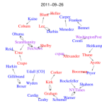
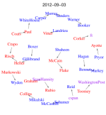
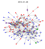
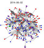
The retweeting and mentions interactions from our data are drawn as directed edges in Figure 1. Given this sequence of network snapshots, we identify particular senators and news agencies that tend to elicit interactions from other accounts (i.e., have many incoming edges relative to how often they tweet), thus revealing their influence on Twitter. Our results further indicate 6 that the proposed approach produces influence measures for the U.S. Senators that correspond more closely with their legislative importance than purely network-based solutions based on the PageRank algorithm.

The remainder of the paper is organized as follows: in Section 2, we introduce the modeling framework and the proposed influence measure. Section 3 presents the algorithm to obtain the model parameter estimates, as well as establish their statistical properties and those of the influence measure. The performance of the model is evaluated on synthetic data sets in Section 4, while the US Senate application is presented in Section 5. Finally, some concluding remarks are drawn in Section 6.

2 The model and the influence measure

We start our presentation by defining some key quantities for future developments. Let $G=(V,L)$ denote the followers network, where $V$ corresponds to the set of nodes of all the Twitter accounts under consideration and $L=\{L_{i,j},1\leq i\neq j\leq n\}$ the edge set between them and captures whether an account foillows another account.. Note that the network is bidirectional in nature and not necessarily symmetric, since account $i$ may follow account $j$, but not vice versa. In principle, $L$ can be dynamically evolving, but in this work we consider $L$ to be static and not changing over time. As explained in the introductory Section, in the Twitter platform, accounts (nodes) can undertake the following three actions: post a new message, retweet a message posted by another account that they follow and finally mention another account that they follow. Further, the vast majority of messages posted, retweeted or mentioned have key terms (wth a $\sharp$ prefix) that identify the topic(s) that are been discussed.

Next, we define the following two key counting processes. Let $N_{j}(t)$ denote the total number of retweets and mentions that account $j$ generates on topic $l$ by time $t$ and by $A_{j}(t,l)$ the total number of posted messages by account $j$ on topic $l$ by time $t$. Define $\alpha_{j}$ to be a parameter that captures the long-term capability of account $j$ to generate responses by other accounts from the content posted, and $\beta_{j}$ a parameter that captures the long term susceptibility of account $j$ to respond (retweet/mention) to the postings of the accounts it follows. We model $\{N_{j}(t,l)\}_{i=1}^{n}$ as a set of counting processes through their hazard rates, using a version of Cox (Andersen and Gill, 1982) proportional hazard model; specifically, the hazard rate $\lambda_{j,l}(t)$ of process $N_{j}(t,l)$ is given by

$$\lambda_{j,l}(t)=\lambda_{0,l}(t)\exp\left(\sum_{i\neq j}L_{ij}(\alpha_{i}+\beta_{j})\log(M_{i}(t,l)+1)\right),$$ (1)

where $M_{j}(t,l)=A_{j}(t,l)+N_{j}(t,l)$ the total number of posting, retweets and mentions for account $j$ on topic $l$ by time $t$. We assume that the parameters $\alpha_{i},\beta_{i}\in(-\infty,\infty)$, since accounts and their users may be positively or negatively inclined towards other accounts, as well as being more keen in joining specific conversations or passively retweeting messages from favorite accounts. The nonparametric baseline component $\lambda_{0,l}(t)$ is time varying. In general, we would expect this baseline to be small for large times $t$, since topics in social media platforms have a high churn rate; they become ”hot” and generate a lot of action over short time scales and afte awhile it stops being discussed. The model posits that account $j$ interacts with other accounts at a baseline level $\lambda_{0,l}(t)$, modulated by its ability to generate responses by accounts in its followers network, as well as its own susceptibility to respond to accounts it follows postings and rebroadcasting of messages. Note that we model the retweet-mention process $N_{j}(t,l)$, since it reflects interactions between nodes and use the total activity process $M_{j}(t,l)$ as a covariate.

To complete the modeling framework, denote the set of topics in the data as $\{1,\ldots,\Gamma\}$. Further, let $\mathcal{T}_{j}^{l}=\left\{T_{j,1}^{l},\ldots,T_{j,n_{j}}^{l}\right\},t=1,\cdots,n_{j},$ denote the set of time points that account $j$ took action (post, retweet, mention) on topic $l$. Finally, for identificaiton purposes, we require one member of the parameter vector $\Omega=(\alpha_{1},\alpha_{2},\ldots,\alpha_{n},\beta_{1},\ldots,\beta_{n})$ to be set to a fixed value, and without loss of generailty we set $\alpha_{1}=0$. Following, (Andersen and Gill, 1982), we employ a partial-likelihood function to obtain estimates of $\Omega$. Specificially, we treat the baseline $\lambda_{0,l}(t)$ as a nuisance parameter and decomposing the full-likelihood to obtain

$$PL=\prod_{1\leq l\leq\Gamma}\left(\prod_{1\leq j\leq n}\prod_{1\leq k\leq n_{j}}\frac{\lambda_{j}(T_{j,k}^{l})}{\sum_{1\leq i\leq n}\lambda_{i}(T_{j,k}^{l})}\right)$$

Plugging the exact form of the hazard rate from (1) into the partial-likelihood function (PL), we get:

$$PL=\prod_{1\leq l\leq\Gamma} \left(\prod_{1\leq j\leq n}\prod_{1\leq k\leq n_{j}}\frac{\exp\left(\sum_{i\neq j}L_{ij}(\alpha_{i}+\beta_{j})\log(M_{i}(T_{j,k}^{l},l)+1)\right)}{\sum_{1\leq i\leq n}\exp\left(\sum_{u\neq i}L_{ui}(\alpha_{u}+\beta_{i})\log(M_{u}(T_{j,k}^{l},l)+1)\right)}\right)$$ (2)

2.1 The Influence Measure

Leveraging the structure of the model, we propose to measure an account’s (node) influence as the total hazard rate change it will bring to its followers. Specifically, for an account $j$ its hazard rate at time $t$ is given by: $H_{j}=\exp\left(\sum_{k\neq j}\log(M_{k}(t)+1)L_{kj}(\alpha_{k}+\beta_{j})\right)$. Further, the contribution of node $i$ is $H_{j}^{(i)}=\exp\left(\log(M_{i}(t)+1)L_{ij}(\alpha_{i}+\beta_{j})\right)$. Then, after some algebra we obtain that the total hazard rate change $i$ brings to its followers can be written as:

$$TH^{(i)}=\sum_{j\neq i}L_{ij}\cdot\exp\left(\log(M_{i}(t)+1)(\alpha_{i}+\beta_{j})\right).$$ (3)

Since $M_{i}(t)$ is a random value, we approximate it by its observed average value, $\bar{M}_{i}$, calculated from the data. Hence, the influence measure becomes

$$\tilde{TH}^{(i)}=\sum_{j\neq i}L_{ij}\cdot\exp\left(\log(\bar{M}_{i}+1)(\alpha_{i}+\beta_{j})\right).$$ (4)

Finally, we express it in a log-scale, so as to linearize the scale and make it compatible with the range of values of the response and susceptibility parameters $\alpha$ and $\beta$:

$$\Xi^{(i)}=\log\left[\sum_{j\neq i}L_{ij}\cdot\exp\left(\log(\bar{M}_{i}+1)(\alpha_{i}+\beta_{j})\right)\right].$$ (5)

3 Computation and Inference

Next, we present a Newton-type algorithm for computing the parameter estimates $\Omega$. The objective function corresponds to the logarithm of the partial likelihood function (2) given by

$$LL=\log(PL)=\sum_{1\leq l\leq\Gamma} \left\{\sum_{1\leq j\leq n}\sum_{1\leq k\leq n_{j}}\sum_{i\neq j}L_{ij}(\alpha_{i}+\beta_{j})\log(M_{i}(T_{j,k}^{l},l)+1)\right.$$ (6)

$$-\sum_{1\leq j\leq n}\sum_{1\leq k\leq n_{j}}\log\left[\sum_{1\leq i\leq n}\exp\left(\sum_{u\neq i}L_{ui}(\alpha_{u}+\beta_{i})\log(M_{u}(T_{j,k}^{l},l)+1)\right)\right]$$

Due to its smoothness we employ Newton’s algorithm that uses the gradient and the Hessian of $LL$. The detailed expressions for the gradient vector $G\equiv\nabla_{\Omega}LL$ and the Hessian $H\equiv\nabla_{\Omega}\nabla_{\Omega}(LL)$ are given in the Appendix.

1:  Initialize the vector $\Omega$ value by $\alpha_{1}=\ldots=\alpha_{n}=\beta_{1}\ldots=\beta_{n}=c=0$

2:  Define $s$ as a positive thresholding constant for the minimum step size

3:  while $t>s$ do

4:     Calculate $G$ by using (9) and (10)

5:     Calculate $H$ by using (11) to (16)

6:     Find the optimum positive $\tau$ value such that $\Omega-\tau\cdot H^{-1}G$ will maximize the log-partial-likelihood (LABEL:LL)

7:     Update $\Omega\leftarrow\Omega-\tau\cdot H^{-1}G$.

8:     In the updated $\Omega$, set $\alpha_{1}=0$.

9:  end while

10:  return  $\Omega$

Algorithm 1 Estimating the parameters by Newton’s algorithm

The steps of the optimization are given in Algorithm 1. As stated in the algorithm, $s$ is a positive constant to judge the convergence of the the Newton’s algorithm. The computational complexity of this algorithm is dominated by the computation of $H$. Denote by $m_{n}=\max_{1\leq j\leq n}\{n_{j}\}$. Based on (9) and (10), it costs $O(\Gamma nm_{n})$ operations to calculate an entry of $G$. Further, siince $G$ is of dimension $2n$, it takes $O(\Gamma n^{2}m_{n})$ to obtain the entire $G$ vector. Analogously, based on (11) to (16), it costs $O(\Gamma nm_{n})$ operations to calculate an entry of $H$, if proper book-keeping is used on the results obtained for the gradient $G$. Further, since $H$ is of dimension $n^{2}$, it takes $O(\Gamma n^{3}m_{n})$ to obtain the entire $H$ matrix. Hence, the overall time complexity for each iteration of the algorithm is of the order $O(\max\{\Gamma n^{3}m_{n}\})$.

4 Properties of the $\hat{\Omega}$ estimates

Next, we establish that the estimator $\hat{\Omega}$ which maximizes (LABEL:LL) will converge to the true parameter $\Omega$ in probability in probability under certain regularity conditions. Before we state the main result, we present some definitions. Let

$$E_{j}(t,\Omega)=\Gamma^{-1}\sum_{l}\lambda_{j,l}(t)=\Gamma^{-1}\sum_{l}\lambda_{0,l}\exp\left(\sum_{i,i\neq j}L_{ij}(\alpha_{i}+\beta_{j})\log(M_{i}(t,l)+1)\right)$$

$$\Phi_{j}=(\phi_{1},\ldots,\phi_{n}):=(\alpha_{1}+\beta_{j},\ldots,\alpha_{n}+\beta_{j})$$

$$\Phi_{j}^{\prime}=(\phi_{1}^{\prime},\ldots,\phi_{n}^{\prime}):=(\alpha_{1}^{\prime}+\beta_{j}^{\prime},\ldots,\alpha_{n}^{\prime}+\beta_{j}^{\prime})^{\prime}$$

$$E_{j}^{(1)}(t,\Omega)=\left(\frac{\partial E_{j}(t,\Omega)}{\partial\phi_{1}},\dots,\frac{\partial E_{j}(t,\Omega)}{\partial\phi_{n}}\right)$$

$$E_{j}^{(1)}(t,\Omega^{\prime})=\left(\frac{\partial E_{j}(t,\Omega^{\prime})}{\partial\phi_{1}^{\prime}},\dots,\frac{\partial E_{j}(t,\Omega^{\prime})}{\partial\phi_{n}^{\prime}}\right)$$

Then, we can establish the following result.

Theorem 1. Suppose there exists time point $t_{0}$, such that all the observed time points satisfy $T_{j,k}^{k}\leq t_{0}$ . Further, for each topic $l$, the observation times $T_{j,k}^{l},1\leq k\leq n_{j}$ are different, for all $1\leq l\leq\Gamma$. (Note however, that for different topics we allow overlap of event occuring times.) Further, we assume that

(A) (Finite interval) $\int_{0}^{t_{0}}\lambda_{0}(u)du<\infty$.

(B) There exists $e(\Omega^{\prime},t)$ such that

$$\sup_{t\in[0,t_{0}],\Omega^{\prime}}\sum_{j}|{E}_{j}(t,\Omega^{\prime})-{e}(\Omega^{\prime},t)|\to_{P}0^{\prime}$$

And if we denote

$$e_{j}^{(1)}(t,\Omega^{\prime})=\left(\frac{\partial e_{j}(t,\Omega^{\prime})}{\partial\phi_{1}^{\prime}},\dots,\frac{\partial e_{j}(t,\Omega^{\prime})}{\partial\phi_{n}^{\prime}}\right)$$

$$e_{j}^{(2)}(t,\Omega^{\prime})=\left(\frac{\partial^{2}e_{j}(t,\Omega^{\prime})}{\partial\phi_{i}^{\prime}\partial\phi_{j}^{\prime}}\right)$$

then also,

$$\sup_{t\in[0,t_{0}],\Omega^{\prime}}\sum_{j}\|{E}_{j}^{(1)}(t,\Omega^{\prime})-{e}^{(1)}(\Omega^{\prime},t)\|\to_{P}0$$

$$\sup_{t\in[0,t_{0}],\Omega^{\prime}}\sum_{j}\|{E}_{j}^{(2)}(t,\Omega^{\prime})-{e}^{(2)}(\Omega^{\prime},t)\|\to_{P}0$$

where again $\|\cdot\|$ is the $L_{2}$ norm of a vector or matrix.

(C) $e(\Omega^{\prime},t)$ is bounded away from zero. $e(\Omega^{\prime},t)$ and $e^{(1)}(\Omega^{\prime},t)$ are continuous functions of $\Omega^{\prime}$, uniformly in $t\in[0,t_{0}]$. $e^{(2)}(\Omega,t)$ is positive definite.

Then, under condistions (A-C), we have that

$$\hat{\Omega}\to_{P}\Omega.$$

The detailed proof is given in the Appendix.

Based on Theorem 1, by leveraging the properties of continuous functions, we can establish the consistency of the proposed inflience measure.

Proposition 1. Let $\Xi(t)=(\Xi^{1}(t),\cdots,\Xi^{n}(t))$ denote the $n$-dimensional vector of influence measures at time $t$. Further, denote by $\hat{\Xi}(t)=(\hat{\Xi}^{1}(t),\cdots,\hat{\Xi}^{n}(t))$ their empirical estimates. Under the conditions of Theorem 1, we have that

$$\left\|\hat{\Xi}(t)-\Xi(t)\right\|\to_{P}0$$ (7)

for any $t\geq 0$.

Based on Theorem 1, the proof of the proposition is straightforward, since each element of the vector $\hat{\Xi}$ is a continuous function of $\hat{\Omega}$.

5 Performance evaluation

In this section, we evaluate the proposed model and influence measure on synthetic data. We start by outlining the data generation mechanism.

Step 1: Building the followers network $L$.
The steps employed for this task are presented next.

• First, for each node $i$, generate $K_{1}(i)$ from a uniform distribution on the integers $\{1,\ldots,K\}$, where $K=\lfloor*n/2\rfloor$ and $\lfloor*\cdot\rfloor$ is the floor function that returns the maximum integer not larger than the value inside.

• Generate $F_{1}(i)$ for node $i$ by randomly sampling $K_{1}(i)$ users from $\{1,\ldots,n\}\backslash\{i\}$ . If $k\in F_{1}(i)$, let $L_{ik}=1$, $1\leq i\leq n$.

• For each node $j$, sample $K_{2}(j)$ uniformly from the set $\{1,\ldots,K\}$. Generate $F_{2}(i)$ for node $j$ by randomly sampling $K_{2}(j)$ users from $\{1,\ldots,n\}\backslash\{j\}$ . If $k\in F_{2}(j)$, let $L_{kj}=1$, $1\leq j\leq n$.

At the end of this procedure, every node in the network has at least one follower and at least an account that it follows.
Step 2. Generate the post, retweets and mentions sequences.
Since the baseline hazard rate $\lambda_{0,l}(t)$ always gets canceled in the partial- likelihood function (2), we select $\lambda_{0,l}(t)$ as $\lambda_{0,l}(t)=a$, whenever $0\leq t\leq t_{0}$ and $\lambda_{0,l}(t)=0$ when $t>t_{0}$, where $a$ is a small positive constant.

We then generate actions on this network withthe following algorithm below for each topic $l\in\{1,\ldots,\Gamma\}$. In this algorithm, we let the nodes send tweets with probability $p$ at each time point $0,1,\ldots,\lfloor*t_{0}\rfloor$, while we generate the retweets and mentions in the standard survial analysis way, by using the hazard rate (1).

1: Initialize Indicator which is the sequence to record the nodes that have mentioned or retweeted as an empty sequence.

2: Initial t=0. Let each node has a tweet with probability $p$.

3: Let each node send out tweets from Binomial$(J,p)$.

4: while $t<t_{0}$ (stopping time for all topics) do

5:    Generate survival time for each node with its hazard rate (1)

6:    Find node $i$ with the shortest time $t_{s}$.

7:    if $t+t_{s}<t_{0}$ then

8:       Update $t$ to be $t+t_{s}$. Record the node that has done this retweet or mention.

9:    end if

10:    if $t+t_{s}>t_{0}$ then

11:       Break

12:    end if

13: end while

14: return  Indicator

Algorithm 2 Generate Group A actions

We first illustrate the performance of the Newton estimation algorithm, on a random network of varying size. We set the parameter $a=0.5$ for the baseline hazard rate and choose a time horizon of $t_{0}=7$, to emulate a week’s worth of data. We also select the parameters $\Omega$ uniformly at random in the interval $[-0.3,0.3]$. With different network sizes $n$ and number of topics generated $\Gamma$, we obtain the following two plots to show the mean squared error of the parameter and influence estimates $\frac{\|\hat{\Omega}-\Omega\|}{\sqrt{2n-1}}$ and $\frac{\|\hat{\Xi}-\Xi\|}{\sqrt{n}}$, where $\|\cdot\|$ corresponds to the $\ell_{2}$ norm of a vector. The results are based on 20 replicates of the underlying followers networks, as well as the actions (postings, retweets and mentions) data.

Figure 2: Mean squared error of the model parameter estimates $\Omega$ (left) and $\Xi$ (right).

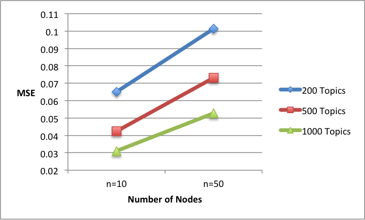
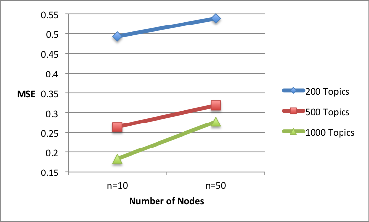
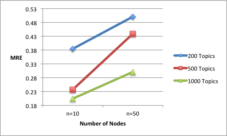
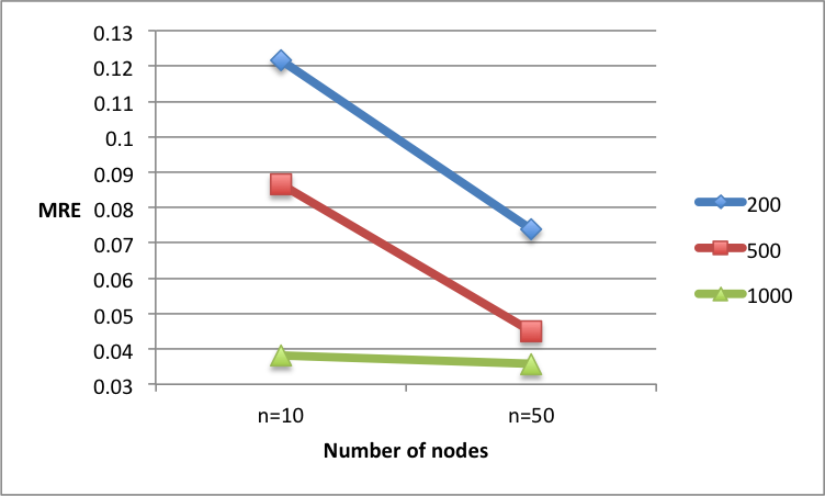
It can be seen that the quality of the estimates improves as a function of the number $\Gamma$ of topics discussed, while it deteriorates as a function of the number of nodes in the followers network $L$. Another way to look at the quality of the estimates, is to examine the relative error of the parameter and influence estimates, given by $\frac{\|\hat{\Omega}-\Omega\|}{\|\Omega\|}$ and $\frac{\|\hat{\Xi}-\Xi\|}{\|\Xi\|}$.

It can be seen in the following Figure that especially the influence measure which is of prime interest in applications, exhibits a small (less than 10%) relative error rate.

Figure 3: Mean relative error of the model parameter estimates $\Omega$ (left) and $\Xi$ (right).

Next, we use a size 10 network, specially constructed to gain insight into the workings of the proposed influence measure. The settings for the data generation are as follows: $\Gamma=500$, $\alpha_{1}=0,\alpha_{2}=-2,\alpha_{3}=\cdots=\alpha_{10}=0.2$ and $\beta_{1}=\cdots=\beta_{10}=0$. Finally, the topology of the followers networks is given in Figure 5.

Since $\alpha_{2}=-2$, node 2 is an “unpopular” one and hence can hardly generate any retweets and mentions of its postings. On the other hand, all nodes have approximately an equal number of followers, which suggests that their ranking according to the PageRank metric (or many other popular ones based on that network) will be approximately similar. The results based on a single realization of the user actions data generation process is shown iin Figure 5. It can be seen that relying on the followers network structure gives a false impression, while the proposed influence measure that incorporates the actions of the accounts provides a more insightful picture.

6 Identifying Influential Senators

Tweets and follower lists are collected using Twitter’s API and consist of approximately 200,000 tweets and 4671 follower links within the set of 120 accounts from April 2009 to July 2014. The retweeting and mentions interactions are drawn in Figure 1, where accounts are registered to 55 Democratic politicians (U.S. Senators and the President of the U.S.), 46 Republican Senators, 2 government organizations (U.S. Army and the Federal Reserve Board), and 16 media outlets, including newspapers (Financial Times, Washington Post, New York Times, Huffington Post), television networks (MSNBC, Fox News, CNN, CSPAN), reporters (Nate Silver (538), Ezra Klein) and television hosts (Bill O’Reilly, Sean Hannity). The figure shows some periods of increased activity, as in the months surrounding the inauguration of President Obama (January 2013), the debate on raising the debt ceiling of the US government and its temporary suspension around April 2013 and the summer of 2014 (soccer World Cup). Note that the sudden increase during the summer of 2014 may be an artifact of rate limiting data acquisition. Specifically, Twitter’s API allows access to only the past $3000$ tweets for any account. As a consequence, for extremely high volume users, like newspapers and television networks, our data traces their Twitter usage for months. For the least active users in our data, 3000 tweets dates back multiple years.

An inspection of actual tweets in Table 1 shows, consistent with Golbeck et al. (2010), that senators tend to retweet and mention as a means of self or legislative promotion. In fact, we see a number of references to legislative activity, such as calls for gun reform, carbon emissions, and references to actual bills on overtime pay, domestic violence protections, among others. Senators often cite news coverage by retweeting or mentioning news media accounts that support their political agenda, which would suggest that the media outlets collectively have enormous influence. This also suggests that Twitter is utilized by senators as part of a larger strategy to build and coalesce public support in order to pass bills through congress.

Table 1: Actual tweets mentioning or retweeting the most influential accounts over from May 15, 2014 to July 3, 2014.

Date	Account	Tweet
05/19/2014	Menendez	“.$@$SenBlumenthal & in #NJ the avg student loan debt is over $29K. It’s unacceptable! #GameofLoans http://t.co/hUJMSeJbfd”
05/23/2014	Cornyn	“RT @nytimes: Former Defense Secretary Gates Is Elected President of the Boy Scouts http://t.co/C7STUSVIP3”
05/27/2104	Blumenthal	“RT $@$msnbc: $@$SenBlumenthal calls for reviving gun reform debate after mass shooting near Santa Barbara: http://t.co/7sqtf1IAFy”
06/02/2014	Markey	“RT $@$washingtonpost: A huge majority of Americans support regulating carbon from power plants http://t.co/lj6ieL5D1Y http://t.co/2CA63hTqmm”
06/17/2014	Markey	“Proud to intro new bill w $@$SenBlumenthal 2 protect domestic violence victims from #gunviolence http://t.co/MsgK40oLiT http://t.co/ynEHrEbh2x”
06/20/2014	Blumenthal	“Proud to stand w/ $@$CoryBooker & others on enhancing rules to reduce truck driver fatigue. Their safety & safety of others is paramount. -RB”
06/20/2014	Markey	“Proud to support our workers and this commonsense bill w $@$SenatorHarkin Keeping Track: Overtime Pay, via $@$nytimes http://t.co/TnAS96Hro5”
06/25/2014	Durbin	“Watch now: $@$OfficialCBC $@$HispanicCaucus $@$CAPAC $@$USProgressives $@$SenatorCardin on racial profiling #MoreThanAProfile http://t.co/ZX0Eu65dgi
06/25/2014	Cardin	“RT $@$TheTRCP: Thank you $@$SenatorCardin for standing with sportsmen today for #CleanWater #protectcleanwater”
06/27/2014	Markey	“Thanks $@$alfranken $@$CoryBooker $@$amyklobuchar $@$SenBlumenthal for joining me in support of community #broadband http://t.co/O8Px2MzrCg”
06/27/2014	Menendez	“Took my first #selfie at #NJs $@$ALJBS! Hope $@$CoryBooker is proud of his NJ Sen colleague. http://t.co/FrEJonUy9d
06/28/2014	Booker	“Thanks Adam RT $@$AIsaacs7 Props to $@$CoryBooker and $@$SenRandPaul for their bipartisanship in introducing their amendment #MedicalMarijuana”

To test these hypotheses and also rigorously compare the proposed influence measure to PageRank applied to the followers networks (which constitutes the backbone of many ranking algorithms of Twitter accounts), we perform a regression analysis to assess how well each measure explains legislative leadership in Congress. Our response variable is the leadership score, published by www.govtrack.us (GovTrack.us, 2014). GovTrack creates the leadership score by applying the PageRank algorithm to the adjacency matrix of bill cosponsorship data. Thus, the leadership score for each senator is a number between $0$ and $1$, where higher values denote greater legislative leadership. The regression model we are interested in is

$$\text{Leadership}=\beta\text{Influence}+\Theta\text{Controls},$$ (8)

where Influence contains the proposed measure and/or PageRank, and Controls includes party affiliation, gender, age, and number of years in the senate. Seniority endows a number of benefits including preferential assignment to committees. Thus, these control variables likely associate strongly with legislative leadership.

To estimate the proposed influence measure, the data is organized into weekly intervals after using the follow-follower relations to construct the adjacency matrix $L$. In Twitter it is common to use “hashtags” or the # symbol followed by a user-specified category to identify context, which, as mentioned in Section 1 can be used as an indicator of different conversations. However, we find that senators do not utilize hashtags often. To overcome this challenge, we follow previous works on Twitter (Hong and Davison, 2010; Ramage et al., 2010) by applying probabilistic topic modeling, which was first introduced in Blei et al. (2003). Extensive work in computer science and applied statistics has led to fast algorithms capable of analyzing extremely big text archives. Due to space constraints, for statistical and algorithmic details on the topic model, see Blei (2012); Blei and Lafferty (2007) and references therein.

Topic modeling applied to the data results in a soft clustering of tweets into groups (topics), which is appropriate since a single tweet could touch on multiple issues. Thus, tweets are assigned to topics that had at least $0.25$ probability. Given the fast moving landscape of social media, new topics are assigned each week, leading to $2770$ topics in total for the entire data set. After preprocessing, we apply Algorithm 1 to estimate the $\alpha$ and $\beta$ parameters for every account using all data. The final influence measure is constructed by computing the influence measure vector $\hat{\Xi}$ over different time intervals to study how influence evolved; i.e. $\hat{\Xi}$ was computed by using the average $M_{i}(\mathcal{T}_{m})$, where $\mathcal{T}_{m}$ denotes the $m-$th time interval of interest.

Figure 4: Weekly Twitter retweet and mention network drawings for the 2014 summer. Top ten most influential accounts are labeled and node sizes are proportional to the estimated influence under the proposed model. The nodes (Twitter accounts) contain democratic senators (blue circles), republican senators (red squares), media (purple triangles), and government agencies (green stars).

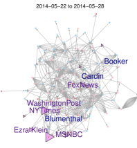
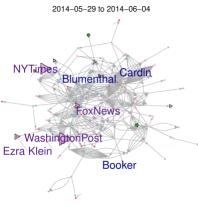
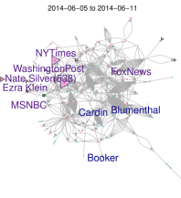
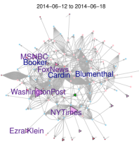
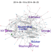
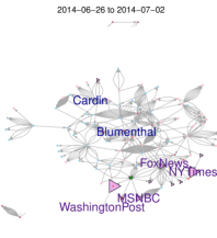
The first time interval $\mathcal{T}_{1}$ we investigate is May 15, 2014 - July 3, 2014, which captures the most active period in our data and also represents a period when rate limiting is not a concern, i.e., the data for even high volume users extends this far. During this time several major events occurred worldwide, including the soccer World Cup, debate on immigration reform, and the Islamic State in Iraq and the Levant (also known as the ISIS or ISIL) began an offensive in northern Iraq. Table 2 shows the top ten most influential accounts under the proposed method and PageRank (Page et al., 1999) calculated from the followers network. Both methods estimate that the Financial Times is the most influential Twitter account, and in general find that the media has an enormous influence that facilitates online conversation between politicians. We see from Figure 4 that these top accounts were actively retweeted and mentioned throughout this period.

Table 2: Top ten rankings according to the proposed model and PageRank from May 15, 2014 - July 3, 2014.

Rank	Proposed Measure	PageRank
1	Financial Times	Financial Times
2	Washington Post	U.S. Army
3	NYTimes	CNN
4	MSNBC	Barack Obama
5	Ezra Klein	CSPAN
6	Fox News	New York Times
7	Cory Booker	Washington Post
8	Ben Cardin	Cory Booker
9	Nate Silver (538)	MSNBC
10	Richard Blumenthal	Wall Street Journal

Table 3: Estimated R-squared values for different regression models, where the proposed measure and/or PageRank is included in the set of independent variables and the influence is computed for the entire data sample. We consistently find that the proposed measure is a better indicator of legislative importance.

Response	Proposed Measure	PageRank	$R^{2}$
			0.311
leadership			0.276
			0.311
			0.114
$log(\frac{\text{leadership}}{1-\text{leadership}})$			0.098
			0.114

Next, we estimate the regression model in Equation 8. We note that Senators Baucus, Kerry, Cowan, Lautenberg, and Chiesa are scored by govtrack.us, but are not in our analysis. Max Baucus and John Kerry are left out, because they vacated their Senate seats to become, respectively, Ambassador to China and U.S. Secretary of State. Mo Cowan succeeded Kerry and was senator from February 1, 2013 to July 16, 2013 until a special election could be held. Cowan chose not to run in the election. Likewise, due to the death of Senator Frank Lautenberg, Jeffrey Chiesa was appointed by Governor Chris Christie to be the junior senator from New Jersey from June 6, 2013 to October 31, 2013. He declined to run in the special election and thus, is also not included in the analysis.

Since the leadership score provided by GovTrack are between $0$ and $1$, we estimate two models. One model uses the raw leadership scores, and another uses $log(\frac{\text{leadership}}{1-\text{leadership}})$ for the response variable. In both cases, as shown in Table 3, we consistently find that the proposed influence measure explains more variation in leadership and when both the proposed and PageRank influence measures are included as independent variables, PageRank does not provide additional explanatory power. Tables 4 and 5 show a significant positive coefficient for the proposed influence measure, meaning that senators who are more influential in Twitter by successfully steering conversation of their colleagues onto particular topics, tend to be more influential in real life in passing legislation. These results are consistent across different time intervals. For instance, in the Appendix we present similar results, where influence is calculated from January 1, 2013 to March 1, 2013 corresponding to sequestration and also from November 1, 2012 to January 31, 2013 corresponding to the president’s reelection and subsequent inauguration.

Table 4: Regression estimates, where the response variable is the raw leadership scores from GovTrack.us and influence is computed for the entire data sample. $R^{2}=0.311$; $F=8.228$ on $5$ and $92$ DF (p-value: $0.000$)

Variable	Estimate	Std. Error	$t$ value	$P(>|t|)$
Intercept	-0.086	0.232	-0.368	0.714
Proposed Influence	0.062	0.028	2.241	0.027
Republican	-0.154	0.039	-3.945	0.000
Age	0.002	0.003	0.923	0.359
Years in Senate	0.007	0.003	2.518	0.014
Male	0.020	0.050	0.395	0.694

Table 5: Regression estimates, where the response variable is $log(\frac{\text{leadership}}{1-\text{leadership}})$, where leaderhip is from GovTrack.us and influence is computed for the entire data sample. $R^{2}=0.114$; $F=2.334$ on $5$ and $92$ DF (p-value: $0.048$)

Variable	Estimate	Std. Error	$t$ value	$P(>|t|)$
Intercept	-3.590	2.604	-1.379	0.171
Proposed Influence	0.437	0.308	1.416	0.160
Republican	-1.112	0.438	-2.538	0.013
Age	0.009	0.029	0.323	0.747
Years in Senate	0.034	0.032	1.063	0.290
Male	0.470	0.563	0.834	0.407

7 Discussion

The goal in this paper was to characterize the influence of users in a large scale social media platform when given information about the detailed actions users take on it. Our comprehensive analysis of the US Senators and related accounts demonstrated that conversations, and in particular the rate of directed activity, between accounts are correlated with their real-world position and influence. We expect similar conclusions to hold broadly for other types of directed interaction data when the nodes form a clearly defined ecosystem or closely knit social group/community.

The modeling and statistical inference issues, associated with these large scale data are different from those in the related literature on network community detection (Kolaczyk, 2009; Fienberg, 2012; Salter-Townshend et al., 2012), where the goal is to identify relatively dense groups of nodes (users), even though the underlying data (observed adjacency matrices) are the same. Relative to other recent work on modeling directed networks, as in Perry and Wolfe (2013), our study has important modeling differences motivated by the online social media platform domain. For instance, our approach incorporates the fundamental differences between actions like retweeting, mentioning, and posting. As a consequence, our final influence measure, which sums all possible influences from the social network, is able to outperform traditional topology driven approaches like PageRank (Page et al., 1999). Perhaps most importantly, given the massive volumes of data generated by platforms like Twitter, we presented a fast estimation algorithm and established statistical properties for the model estimates and those of the final influence measure.

These results suggest that the proposed model can be a relatively straightforward technique to identifying influential individuals within Twitter ecosystems, and that it can complement the significantly more involved text mining based content analysis of the raw messages for related tasks (Taddy, 2013).

8 Proofs

8.1 Expressions for the gradient vector and Hessian matrix of the $LL$ function

Some rather straightforward algebra yields the following expressions for the elements of the gradient vector $G\equiv\nabla_{\Omega}LL$:

$$\frac{\partial LL}{\partial\alpha_{i}}=\sum_{1\leq l\leq\Gamma} \left\{\sum_{1\leq j\leq n,j\neq i}\sum_{1\leq k\leq n_{j}}L_{ij}\log(M_{i}(T_{j,k}^{l},l)+1)\right.$$ (9)

$$\left.-\sum_{1\leq j\leq n}\sum_{1\leq k\leq n_{j}}\frac{\sum_{v\neq i}L_{iv}\log(M_{i}(T_{j,k}^{l},l)+1)\exp\left(\sum_{u\neq v}L_{uv}(\alpha_{u}+\beta_{v})\log(M_{u}(T_{j,k}^{l},l)+1)\right)}{\sum_{1\leq v\leq n}\exp\left(\sum_{u\neq v}L_{uv}(\alpha_{u}+\beta_{v})\log(M_{u}(T_{j,k}^{l},l)+1)\right)}\right\}$$

for $2\leq i\leq n$, and

$$\frac{\partial LL}{\partial\beta_{j}}=\sum_{1\leq l\leq\Gamma} \left\{\sum_{1\leq k\leq n_{j}}\sum_{i\neq j}L_{ij}M_{i}(T_{j,k}^{l},l)\right.$$ (10)

$$\left.-\sum_{1\leq s\leq n}\sum_{1\leq k\leq n_{s}}\frac{\left(\sum_{u\neq j}L_{uj}\log(M_{u}(T_{s,k}^{l},l)+1)\right)\exp\left(\sum_{u\neq j}L_{uj}(\alpha_{u}+\beta_{j})\log(M_{u}(T_{s,k}^{l},l)+1)\right)}{\sum_{1\leq v\leq n}\exp\left(\sum_{u\neq v}L_{uv}(\alpha_{u}+\beta_{v})\log(M_{u}(T_{s,k}^{l},l)+1)\right)}\right\}$$

for $1\leq j\leq n$.

Next, we obtain the necessary expressions for the Hessian matrix $H(LL)$. We start by computing the sub-matrix of $H$ that includes the second partial derivatives of $LL$ with respect to the $\alpha$ parameters. We get

$$\frac{\partial^{2}LL}{\partial\alpha_{i}^{2}}=\sum_{1\leq l\leq\Gamma} \left\{-\sum_{1\leq j\leq n}\sum_{1\leq k\leq n_{j}}\frac{\sum_{v\neq i}L_{iv}\log(M_{i}^{2}(T_{j,k}^{l},l)+1)\exp\left(\sum_{u\neq v}L_{uv}(T_{j,k}^{l})(\alpha_{u}+\beta_{v})\log(M_{u}(T_{j,k}^{l},l)+1)\right)}{\sum_{1\leq v\leq n}\exp\left(\sum_{u\neq v}L_{uv}(\alpha_{u}+\beta_{v})\log(M_{u}(T_{j,k}^{l},l)+1)\right)}\right.$$ (11)

$$\left.+\sum_{1\leq j\leq n}\sum_{1\leq k\leq n_{j}}\frac{\left[\sum_{v\neq i}L_{iv}\log(M_{i}(T_{j,k}^{l},l)+1)\exp\left(\sum_{u\neq v}L_{uv}(\alpha_{u}+\beta_{v})\log(M_{u}(T_{j,k}^{l},l)+1)\right)\right]^{2}}{\left[\sum_{1\leq v\leq n}\exp\left(\sum_{u\neq v}L_{uv}(\alpha_{u}+\beta_{v})\log(M_{u}(T_{j,k}^{l},l)+1)\right)\right]^{2}}\right\}$$

When $i\neq q$, we similarly have

$$\frac{\partial^{2}LL}{\partial\alpha_{i}\partial\alpha_{q}}=\sum_{1\leq l\leq\Gamma} \left\{-\sum_{1\leq j\leq n}\sum_{1\leq k\leq n_{j}}\frac{\sum_{v\neq i,q}L_{iv}\log(M_{i}(T_{j,k}^{l},l)+1)L_{qv}\log(M_{q}(T_{j,k}^{l},l)+1)}{\sum_{1\leq v\leq n}\exp\left(\sum_{u\neq v}L_{uv}(\alpha_{u}+\beta_{v})\log(M_{u}(T_{j,k}^{l},l)+1)\right)}\right.$$ (12)

$$\cdot\exp\left(\sum_{u\neq v}L_{uv}(\alpha_{u}+\beta_{v})\log(M_{u}(T_{j,k}^{l},l)+1)\right)$$

$$+\sum_{1\leq j\leq n}\sum_{1\leq k\leq n_{j}}\frac{\sum_{v\neq i}L_{iv}\log(M_{i}(T_{j,k}^{l},l)+1)\exp\left(\sum_{u\neq v}L_{uv}(\alpha_{u}+\beta_{v})\log(M_{u}(T_{j,k}^{l},l)+1)\right)}{\left[\sum_{1\leq v\leq n}\exp\left(\sum_{u\neq v}L_{uv}(\alpha_{u}+\beta_{v})\log(M_{u}(T_{j,k}^{l},l)+1)\right)\right]^{2}}$$

$$\cdot\left[\sum_{v\neq q}L_{qv}\log(M_{q}(T_{j,k}^{l},l)+1)\exp\left(\sum_{u\neq v}L_{uv}(\alpha_{u}+\beta_{v})\log(M_{u}(T_{j,k}^{l},l)+1)\right)\right]$$

Next, we obtain the sub-matrix of $H$ that includes the second partial derivatives of $LL$ with respect to the $\beta$ parameters and get

$$\frac{\partial^{2}LL}{\partial\beta_{j}^{2}}=\sum_{1\leq l\leq\Gamma} \left\{\sum_{1\leq s\leq n}\sum_{1\leq k\leq n_{s}}\frac{\left[\left(\sum_{u\neq j}L_{uj}\log(M_{u}(T_{s,k}^{l},l)+1)\right)\exp\left(\sum_{u\neq j}L_{uj}(\alpha_{u}+\beta_{j})\log(M_{u}(T_{s,k}^{l},l)+1)\right)\right]^{2}}{\left[\sum_{1\leq v\leq n}\exp\left(\sum_{u\neq v}L_{uv}(\alpha_{u}+\beta_{v})\log(N_{u}(T_{s,k}^{l},l)+1)\right)\right]^{2}}\right.$$ (13)

$$\left.-\sum_{1\leq s\leq n}\sum_{1\leq k\leq n_{s}}\frac{\left(\sum_{u\neq j}L_{uj}\log(M_{u}(T_{s,k}^{l},l)+1)\right)^{2}\exp\left(\sum_{u\neq j}L_{uj}(\alpha_{u}+\beta_{j})\log(M_{u}(T_{s,k}^{l},l)+1)\right)}{\sum_{1\leq v\leq n}\exp\left(\sum_{u\neq v}L_{uv}(\alpha_{u}+\beta_{v})\log(M_{u}(T_{s,k}^{l},l)+1)\right)}\right\}$$

for $1\leq j\leq n$. When $j\neq q$, we can similarly have

$$\frac{\partial^{2}LL}{\partial\beta_{j}\partial\beta_{q}}=\sum_{1\leq l\leq\Gamma} \left\{\sum_{1\leq s\leq n}\sum_{1\leq k\leq n_{s}}\frac{\left(\sum_{u\neq j}L_{uj}\log(M_{u}(T_{s,k}^{l},l)+1)\right)\exp\left(\sum_{u\neq j}L_{uj}(\alpha_{u}+\beta_{j})\log(M_{u}(T_{s,k}^{l},l)+1)\right)}{\left[\sum_{1\leq v\leq n}\exp\left(\sum_{u\neq v}L_{uv}(\alpha_{u}+\beta_{v})\log(M_{u}(T_{s,k}^{l},l)+1)\right)\right]^{2}}\right.$$ (14)

$$\left.\cdot\left(\sum_{q\neq j}L_{uq}\log(M_{u}(T_{s,k}^{l},l)+1)\right)\exp\left(\sum_{u\neq q}L_{uj}(\alpha_{u}+\beta_{q})\log(M_{u}(T_{s,k}^{l},l)+1)\right)\right\}$$

Finally, we provide expressions for the cross-partials

$$\frac{\partial^{2}LL}{\partial\alpha_{i}\partial\beta_{i}}=\sum_{1\leq l\leq\Gamma} \left\{\sum_{1\leq s\leq n}\sum_{1\leq k\leq n_{s}}\frac{\left(\sum_{u\neq i}L_{ui}\log(M_{u}(T_{s,k}^{l},l)+1)\right)\exp\left(\sum_{u\neq i}L_{ui}(\alpha_{u}+\beta_{i})\log(M_{u}(T_{s,k}^{l},l)+1)\right)}{\left[\sum_{1\leq v\leq n}\exp\left(\sum_{u\neq v}L_{uv}(\alpha_{u}+\beta_{v})\log(M_{u}(T_{s,k}^{l},l)+1)\right)\right]^{2}}\right.$$ (15)

$$\left.\cdot\sum_{v\neq i}L_{iv}\log(M_{i}(T_{s,k}^{l},l)+1)\exp\left(\sum_{u\neq v}L_{uv}(\alpha_{u}+\beta_{v})\log(M_{u}(T_{s,k}^{l},l)+1)\right)\right\}$$

When $i\neq j$,

$$\frac{\partial^{2}LL}{\partial\alpha_{i}\partial\beta_{j}} =\sum_{1\leq l\leq\Gamma}\left\{\sum_{1\leq s\leq n}\sum_{1\leq k\leq n_{s}}\frac{\left(\sum_{u\neq j}L_{uj}\log(M_{u}(T_{s,k}^{l},l)+1)\right)\exp\left(\sum_{u\neq j}L_{uj}(\alpha_{u}+\beta_{j})\log(M_{u}(T_{s,k}^{l},l)+1)\right)}{\left[\sum_{1\leq v\leq n}\exp\left(\sum_{u\neq v}L_{uv}(\alpha_{u}+\beta_{v})\log(M_{u}(T_{s,k}^{l},l)+1)\right)\right]^{2}}\right.$$ (16)

$$\cdot\sum_{v\neq i}L_{iv}\log(M_{i}(T_{s,k}^{l},l)+1)\exp\left(\sum_{u\neq v}L_{uv}(\alpha_{u}+\beta_{v})\log(M_{u}(T_{s,k}^{l},l)+1)\right)$$

$$\left.-\sum_{1\leq s\leq n}\sum_{1\leq k\leq n_{s}}\frac{\left(\sum_{u\neq j}L_{uj}\log(M_{u}(T_{s,k}^{l},l)+1)\right)L_{ij}\log(M_{i}(T_{s,k}^{l},l)+1)\exp\left(\sum_{u\neq j}L_{uj}(\alpha_{u}+\beta_{j})\log(M_{u}(T_{s,k}^{l},l)+1)\right)}{\sum_{1\leq v\leq n}\exp\left(\sum_{u\neq v}L_{uv}(\alpha_{u}+\beta_{v})\log(M_{u}(T_{s,k}^{l},l)+1)\right)}\right\}$$

8.2 Proof of Theorem 1

Note that since the baseline hazard rate $\lambda_{0,l}(t)$ is canceled out in the partial likelihood and the estimation of the parameter vector $\Omega$ will not depend on its value, in the rest of the proof, we can safelyl ignore it. Next, consider the process

$$X(\Omega^{\prime},t)=\Gamma^{-1}(LL(\Omega^{\prime},t)-LL(\Omega,t)),$$

where recall that $\Gamma$ denotes the number of topics under consideration. Then, given $\Omega$, it is straightforward to see that $\hat{\Omega}$ is the unique maximum point (with probability going to 1) of $X(\Omega,t_{0})$ (Andersen and Gill, 1982) and $X(\Omega,t_{0})$ is a concave function. To simplify notation, we let $TN(t,l)=\sum_{i}N_{i}(t,l)$. Then, we can expand $X(\Omega^{\prime},t)$ as:

$$X(\Omega^{\prime},t) =\Gamma^{-1}\left\{\sum_{l}\int_{0}^{t}\sum_{j}\sum_{i,i\neq j}L_{ij}(\alpha_{i}^{\prime}+\beta_{j}^{\prime}-\alpha_{i}-\beta_{j})\log(M_{i}(u,l)+1)dN_{j}(u,l)\right.$$

$$\left.-\int_{0}^{t}\log\left\{\frac{\sum_{j}\exp\left(\sum_{i,i\neq j}L_{ij}(\alpha_{i}^{\prime}+\beta_{j}^{\prime})\log(M_{i}(u,l)+1)\right)}{\sum_{j}\exp\left(\sum_{i,i\neq j}L_{ij}(\alpha_{i}+\beta_{j})\log(M_{i}(u,l)+1))\right)}\right\}dTN(u,l)\right\}$$

Notice that by the definitions of the hazard rates, by defining

$$E_{j}(t,l)=N_{j}(t,l)-\int_{0}^{t}\exp\left(\sum_{i,i\neq j}L_{ij}(u)(\alpha_{i}+\beta_{j})\log(M_{i}(u,l)+1)\right)du$$ (17)

$j=1,\ldots,n$, we can easily establish that $E_{j}(t,l)$s are local martingales on the time interval $[0,t_{0}]$. Then, in $X(\Omega^{\prime},t)$, we replace $dN_{j}(t,l)$ with the hazard rates of $N_{j}(t,l)$, which is

$$\exp\left(\sum_{i\neq j}L_{ij}(t)(\alpha_{i}+\beta_{j})\log(M_{i}(t,l)+1)\right)$$

Then, we can get

$$A(\Omega^{\prime},t) =\Gamma^{-1}\left\{\sum_{l}\int_{0}^{t}\sum_{j}\sum_{i,i\neq j}L_{ij}(\alpha_{i}^{\prime}+\beta_{j}^{\prime}-\alpha_{i}-\beta_{j})\log(M_{i}(u,l)+1)\exp\left(\sum_{i\neq j}L_{ij}(t)(\alpha_{i}+\beta_{j})\log(M_{i}(t,l)+1)\right)du\right.$$ (18)

$$\left.-\int_{0}^{t}\log\left\{\frac{\sum_{j}\exp\left(\sum_{i,i\neq j}L_{ij}(\alpha_{i}^{\prime}+\beta_{j}^{\prime})\log(M_{i}(u,l)+1)\right)}{\sum_{j}\exp\left(\sum_{i,i\neq j}L_{ij}(\alpha_{i}+\beta_{j})\log(M_{i}(u,l)+1)\right)}\right\}\left(\sum_{j}\exp\left(\sum_{i\neq j}L_{ij}(\alpha_{i}+\beta_{j})\log(M_{i}(t,l)+1)\right)\right)du\right\}$$

Some algebra shows that $X(\Omega^{\prime},t)-A(\Omega^{\prime},\cdot)$ can be written as a finite sum of the square integrable local martingales $E_{j}(t,l)$ in (17). Then, the lastter is also a local square integrable martingale. By Theorem 2.4.3 in (Fleming and Harrington, 2013), we have

$$<X(\Omega^{\prime},t)-A(\Omega^{\prime},t),X(\Omega^{\prime},t)-A(\Omega^{\prime},t)>=B(\Omega^{\prime},t),$$

where

$$B(\Omega^{\prime},t)=\Gamma^{-2}\sum_{l}\sum_{j}\ \int_{0}^{t}S_{j}(u,l)^{2}\lambda_{0}\exp\left(\sum_{i,i\neq j}L_{ij}(\alpha_{i}+\beta_{j})\log(M_{i}(u,l)+1)\right)du,$$ (19)

where in (19) above, $S_{j}(u,l)$ is given by

$$S_{j}(u,l)=\sum_{i,i\neq j}L_{ij}(\alpha_{i}^{\prime}+\beta_{j}^{\prime}-\alpha_{i}-\beta_{j})\log(M_{i}(u,l)+1)-\log\left\{\frac{\sum_{j}\exp\left(\sum_{i,i\neq j}L_{ij}(\alpha_{i}^{\prime}+\beta_{j}^{\prime})\log(M_{i}(u,l)+1)\right)}{\sum_{j}\exp\left(\sum_{i,i\neq j}L_{ij}(\alpha_{i}+\beta_{j})\log(M_{i}(u,l)+1)\right)}\right\}$$

Since $\Gamma\cdot B(\Omega^{\prime},\cdot)$ converges in probability to some finite quantity (by the law of large numbers, depending on $\Omega$), $X(\Omega^{\prime},t)$ should converge to the same limit as $A(\Omega^{\prime},t)$ for each $\Omega^{\prime}$ (if $A(\Omega^{\prime},t)$ converges). Note that by using the notation employed in Condition (A) and (B) in Theorem 1, $A(\Omega^{\prime},t)$ can be simplified to

$$A(\Omega^{\prime},t)= \int_{0}^{t}\left[\sum_{j}(\Phi_{j}^{\prime}-\Phi_{j})^{\prime}E_{j}^{(1)}(u,\Omega)-\log\left\{\frac{\sum_{j}E_{j}(u,\Omega^{\prime})}{\sum_{j}E_{j}(u,\Omega)}\right\}\sum_{j}E_{j}(u,\Omega)\right]du$$

It follows that by conditions (A), (B) and (C), for each $\Omega^{\prime}$, as $\Gamma\to\infty$,

$$A(\Omega^{\prime},t_{0})\to_{P}P(\Omega^{\prime},t_{0}),$$

where

$$P(\Omega^{\prime},t_{0})=\int_{0}^{t_{0}}\left[\sum_{j}(\Phi_{j}^{\prime}-\Phi_{j})^{\prime}e_{j}^{(1)}(u,\Omega)-\log\left\{\frac{\sum_{j}e_{j}(u,\Omega^{\prime})}{\sum_{j}e_{j}(u,\Omega)}\right\}\sum_{j}e_{j}(u,\Omega)\right]du$$

Now, we want to establish that $P(\Omega^{\prime},t_{0})$ remains convex. We evaluate the first and second derivative of $P_{1}(\Omega^{\prime},t_{0})$ to show its convexity. By Condition (C), we can compute the first derivatives as

$$\frac{\partial P(\Omega^{\prime},t_{0})}{\partial\beta_{j}^{\prime}}=\int_{0}^{t_{0}}\left[e_{j}^{(1)}(u,\Omega)-e_{j}^{(1)}(u,\Omega^{\prime})\frac{\sum_{j}e_{j}(u,\Omega)}{\sum_{j}e_{j}(u,\Omega^{\prime})}\right]du$$

and

$$\frac{\partial P(\Omega^{\prime},t_{0})}{\partial\alpha_{i}^{\prime}}=\int_{0}^{t_{0}}\left[\sum_{j}I_{i}^{\prime}e_{j}^{(1)}(u,\Omega)-(\alpha_{1}^{\prime},\ldots,\alpha_{n}^{\prime})^{\prime}\sum_{j}I_{i}^{\prime}e_{j}^{(1)}(u,\Omega^{\prime})\frac{\sum_{j}e_{j}(u,\Omega)}{\sum_{j}e_{j}(u,\Omega^{\prime})}\right]du$$

where $I_{i}$ is a $n$-dimensional vector with all zeros expect one on the $i$-th entry.

Note that the above parital derivatives are all zero at $\Omega^{\prime}=\Omega$. Further, the second derivatives are

$$\int_{0}^{t_{0}}\left[e_{j}^{(2)}(u,\Omega)+e_{j}^{(1)}(u,\Omega)^{\otimes 2}\frac{\sum_{j}e_{j}(u,\Omega)}{\sum_{j}e_{j}(u,\Omega^{\prime})}\right]du,$$

which is a positive semidefinite matrix for any $\Omega^{\prime}$ and positive definite at $\Omega$. Thus, $X(\Omega^{\prime},t_{0})$ converges in probability to a convex function of $\Omega^{\prime}$ with a unique maximum at $\Omega$. Since $\hat{\Omega}$ maximizes the concave function $X(\Omega^{\prime},t_{0})$, it follows by a standard result in convex analysis (Rockafellar, 1970) that $\hat{\Omega}\to_{P}\Omega$. This completes the proof of the Theorem.

9 Additional Senator Results

Table 6 shows the top ten most influential accounts under the proposed method for different time periods. We see consistent results with the findings from summer 2014. Important newspapers like the Financial Times and Washington Post still appear in the top ten when utilizing the full data. Other prominent accounts include senators that have leadership positions, like Harry Reid (Senate Majority Leader) and several others with high profile committee chairmanships or ranking appointments.

Table 6: Top ten rankings under the proposed model for different time intervals.

Rank	Sequestration	2014 Inauguration	Entire Data
1	Leahy	Leahy	Financial Times
2	Grassley	Grassley	Grassley
3	Mikulski	Begich	Leahy
4	Begich	Mikulski	Cruz
5	Shaheen	Johanns	Washington Post
6	McCaskill	Reid	Reid
7	Reid	McCaskill	Begich
8	Blunt	Graham	Mikulski
9	Graham	Shaheen	Ezra Klein
10	Collins	Hagan	Schatz

Tables 7 and 8 show regression results for the sequestration period, and Tables 9 and 10 show regression results for the inauguration period. The results are consistent with the results presented in the main text. Regressing directly on the leadership scores shows a strongly significant and positive coefficient for the proposed influence measure. The regressions with transformed leadership scores show effects are moderately significant.

Table 7: Regression estimates, where the response variable is the raw leadership scores from GovTrack.us and influence is computed from January 1, 2013 to March 1, 2013. $R^{2}=0.327$; $F=8.839$ on $5$ and $92$ DF (p-value: $0.000$)

Variable	Estimate	Std. Error	$t$ value	$P(>|t|)$
Intercept	-0.153	0.228	-0.669	0.505
Proposed Influence	0.074	0.028	2.689	0.009
Republican	-0.153	0.039	-3.960	0.000
Age	0.002	0.003	0.833	0.407
Years in Senate	0.007	0.003	2.532	0.013
Male	0.020	0.050	0.397	0.692

Table 8: Regression estimates, where the response variable is $log(\frac{\text{leadership}}{1-\text{leadership}})$, where leaderhip is from GovTrack.us and influence is computed from January 1, 2013 to March 1, 2013. $R^{2}=0.119$; $F=2.466$ on $5$ and $92$ DF (p-value: $0.038$)

Variable	Estimate	Std. Error	$t$ value	$P(>|t|)$
Intercept	-3.925	2.574	-1.525	0.131
Proposed Influence	0.504	0.312	1.614	0.110
Republican	-1.103	0.437	-2.526	0.013
Age	0.008	0.029	0.267	0.790
Years in Senate	0.033	0.031	1.062	0.291
Male	0.465	0.561	0.830	0.409

Table 9: Regression estimates, where the response variable is the raw leadership scores from GovTrack.us and influence is computed from November 1, 2012 to January 31, 2013. $R^{2}=0.328$; $F=8.839$ on $5$ and $92$ DF (p-value: $0.000$)

Variable	Estimate	Std. Error	$t$ value	$P(>|t|)$
Intercept	-0.132	0.220	-0.597	0.552
Proposed Influence	0.072	0.026	2.726	0.008
Republican	-0.154	0.039	-3.978	0.000
Age	0.002	0.003	0.797	0.427
Years in Senate	0.007	0.003	2.616	0.010
Male	0.020	0.050	0.395	0.693

Table 10: Regression estimates, where the response variable is $log(\frac{\text{leadership}}{1-\text{leadership}})$, where leaderhip is from GovTrack.us and influence is computed from November 1, 2012 to January 31, 2013. $R^{2}=0.117$; $F=2.402$ on $5$ and $92$ DF (p-value: $0.043$)

Variable	Estimate	Std. Error	$t$ value	$P(>|t|)$
Intercept	-3.578	2.495	-1.434	0.155
Proposed Influence	0.452	0.297	1.521	0.132
Republican	-1.105	0.437	-2.527	0.013
Age	0.007	0.029	0.255	0.800
Years in Senate	0.035	0.031	1.113	0.269
Male	0.460	0.561	0.819	0.415

REFERENCES

- (1)
- Andersen and Gill (1982) Andersen, P. K., and Gill, R. D. (1982), “Cox’s regression model for counting processes: a large sample study,” The annals of statistics, pp. 1100–1120.
- Blei (2012) Blei, D. M. (2012), “Probabilistic topic models,” Communications of the ACM, 55(4), 77–84.
- Blei and Lafferty (2007) Blei, D. M., and Lafferty, J. D. (2007), “A correlated topic model of science,” The Annals of Applied Statistics, pp. 17–35.
- Blei et al. (2003) Blei, D. M., Ng, A. Y., and Jordan, M. I. (2003), “Latent dirichlet allocation,” the Journal of machine Learning research, 3, 993–1022.
- Bulearca and Bulearca (2010) Bulearca, M., and Bulearca, S. (2010), “Twitter: a viable marketing tool for SMEs?,” Global Business and Management Research: An International Journal, 2(4), 296–309.
- Cha et al. (2010) Cha, M., Haddadi, H., Benevenuto, F., and Gummadi, P. K. (2010), “Measuring User Influence in Twitter: The Million Follower Fallacy.,” ICWSM, 10, 10–17.
-
Fienberg (2012)
Fienberg, S. E. (2012), “A Brief History of
Statistical Models for Network Analysis and Open Challenges,” Journal
of Computational and Graphical Statistics, 21(4), 825–839.
http://www.tandfonline.com/doi/abs/10.1080/10618600.2012.738106 -
Fleming and Harrington (2013)
Fleming, T., and Harrington, D. (2013), Counting Processes and Survival Analysis, Wiley
Series in Probability and Statistics Wiley.
http://books.google.com/books?id=i85dAAAACAAJ - Gayo-Avello et al. (2011) Gayo-Avello, D., Metaxas, P. T., and Mustafaraj, E. (2011), Limits of electoral predictions using twitter.,, in ICWSM.
Golbeck et al. (2010)
Golbeck, J., Grimes, J. M., and Rogers, A. (2010), “Twitter use by the U.S. Congress,” Journal of
the American Society for Information Science and Technology,
61(8), 1612–1621.
http://dx.doi.org/10.1002/asi.21344 - GovTrack.us (2014) GovTrack.us (2014), “GovTrack.us: Tracking the United States Congress,”, https://www.GovTrack.us. Accessed: 2014-10-26.
- Hong and Davison (2010) Hong, L., and Davison, B. D. (2010), Empirical study of topic modeling in twitter,, in Proceedings of the First Workshop on Social Media Analytics, ACM, pp. 80–88.
Kleinberg (1999)
Kleinberg, J. M. (1999), “Authoritative
sources in a hyperlinked environment,” J. ACM, 46(5), 604–632.
www.cs.cornell.edu/home/kleinber/auth.pdf - Klout (2014) Klout (2014), “Klout — Be Known for What you Love,”, www.Klout.com. Accessed: 2014-11-01.
- Kolaczyk (2009) Kolaczyk, E. D. (2009), Statistical Analysis of Network Data: Methods and Models, Springer Series in Statistics, New York, NY, USA: Springer Publishing Company, Incorporated.
- Kwak et al. (2010) Kwak, H., Lee, C., Park, H., and Moon, S. (2010), What is Twitter, a social network or a news media?,, in Proceedings of the 19th international conference on World wide web, ACM, pp. 591–600.
- Page et al. (1999) Page, L., Brin, S., Motwani, R., and Winograd, T. (1999), “The PageRank citation ranking: Bringing order to the web.,” , .
- PeerIndex (2014) PeerIndex (2014), “PeerIndex – Think People,”, www.PeerIndex.com. Accessed: 2014-11-01.
- Perry and Wolfe (2013) Perry, P. O., and Wolfe, P. J. (2013), “Point process modelling for directed interaction networks,” Journal of the Royal Statistical Society: Series B (Statistical Methodology), 75(5), 821–849.
Ramage et al. (2010)
Ramage, D., Dumais, S., and Liebling, D. (2010), Characterizing Microblogs with Topic Models,, in Proc. ICWSM 2010, American Association for Artificial Intelligence.
http://research.microsoft.com/apps/pubs/default.aspx?id=131777 -
Rockafellar (1970)
Rockafellar, R. (1970), Convex
Analysis, Convex Analysis Princeton University Press.
http://books.google.com/books?id=1TiOka9bx3sC - Salter-Townshend et al. (2012) Salter-Townshend, M., White, A., Gollini, I., and Murphy, T. B. (2012), “Review of statistical network analysis: models, algorithms, and software,” Statistical Analysis and Data Mining, 5(4), 243–264.
Taddy (2013)
Taddy, M. (2013), “Measuring Political
Sentiment on Twitter: Factor Optimal Design for Multinomial Inverse
Regression,” Technometrics, 55(4), 415–425.
http://dx.doi.org/10.1080/00401706.2013.778791 - Trusov et al. (2010) Trusov, M., Bodapati, A. V., and Bucklin, R. E. (2010), “Determining influential users in internet social networks,” Journal of Marketing Research, 47(4), 643–658.
- Twitter (2014) Twitter, I. (2014), “About Twitter, Inc.,”, https://about.twitter.com/company. Accessed: 2014-09-19.
- Weng et al. (2010) Weng, J., Lim, E.-P., Jiang, J., and He, Q. (2010), Twitterrank: finding topic-sensitive influential twitterers,, in Proceedings of the third ACM international conference on Web search and data mining, ACM, pp. 261–270.