Solving Large-Scale Robust Stability Problems by Exploiting the Parallel Structure of Polya’s Theorem

Reza Kamyar, Matthew M. Peet and Yulia Peet Manuscript received November 21, 2011; revised September 24, 2012; accepted February 26, 2013. This work was supported entirely by funding from the National Science Foundation under Award CMMI-1100376. Recommended by XXXX.R. Kamyar is with the Department of Mechanical Engineering, Cybernetic Systems and Controls Laboratory, Arizona State University, Tempe, AZ 85281 USA (e-mail: rkamyar@asu.edu ).M. M. Peet and Y. Peet are with the School for Engineering of Matter, Transport, and Energy, Engineering Research Center, Arizona State University, Tempe, AZ 85281 USA (e-mail: mpeet@asu.edu; ypeet@asu.edu). Color versions of one or more of the figures in this paper are available online at http://ieeexplore.ieee.org.Digital Object Identifier 10.1109/TAC.2013.2253253
Abstract

In this paper, we propose a distributed computing approach to solving large-scale robust stability problems on the simplex. Our approach is to formulate the robust stability problem as an optimization problem with polynomial variables and polynomial inequality constraints. We use Polya’s theorem to convert the polynomial optimization problem to a set of highly structured Linear Matrix Inequalities (LMIs). We then use a slight modification of a common interior-point primal-dual algorithm to solve the structured LMI constraints. This yields a set of extremely large yet structured computations. We then map the structure of the computations to a decentralized computing environment consisting of independent processing nodes with a structured adjacency matrix. The result is an algorithm which can solve the robust stability problem with the same per-core complexity as the deterministic stability problem with a conservatism which is only a function of the number of processors available. Numerical tests on cluster computers and supercomputers demonstrate the ability of the algorithm to efficiently utilize hundreds and potentially thousands of processors and analyze systems with 100+ dimensional state-space. The proposed algorithms can be extended to perform stability analysis of nonlinear systems and robust controller synthesis.

Index Terms:
Robust stability, Polynomial optimization, Large-scale systems, Decentralized computing

I Introduction

This paper addresses the problem of stability of large-scale systems with several unknown parameters. Control system theory when applied in practical situations often involves the use of large state-space models, typically due to inherent complexity of the system, the interconnection of subsystems, or the reduction of an infinite-dimensional or PDE model to a finite-dimensional approximation. One approach to dealing with such large scale models has been to use model reduction techniques such as balanced truncation [1]. However, the use of model reduction techniques are not necessarily robust and can result in arbitrarily large errors. In addition to large state-space, practical problems often contain uncertainty in the model due to modeling errors, linearization, or fluctuation in the operating conditions. The problem of stability and control of systems with uncertainty has been widely studied. See, e.g. the texts [2, 3, 4, 5]. However, a limitation of existing computational methods for analysis and control of systems with uncertainty is high complexity. This is a consequence of fact that the problem of robust stability of systems with parametric uncertainty is known to be NP-hard [6, 7]. The result is that for systems with parametric uncertainty and with hundreds of states, existing algorithms will fail with the primary point of failure usually being lack of unallocated memory.

In this paper, we seek to distribute the computation laterally over an array of processors within the context of existing computational resources. Specifically, we seek to utilize cluster-computing, supercomputing and Graphics Processing Unit (GPU)-computing architectures. When designing algorithms to run in a parallel computing environment, one must both synchronize computational tasks among the processors while minimizing communication overhead among the processors. This can be difficult, as each architecture has a specific communication graph. we account for communication by explicitly modeling the required communication graph between processors. This communication graph is then mapped to the processor architecture using the Message-Passing Interface (MPI) [8]. While there are many algorithms for robust stability analysis and control of linear systems, ours is the first which explicitly accounts for the processing architecture in the emerging multi-core computing environment.

Our approach to robust stability is based on the well-established use of parameter-dependent Quadratic-In-The-State (QITS) Lyapunov functions. The use of parameter-dependent Lyapunov QITS functions eliminates the conservativity associated with e.g. quadratic stability [9], at the cost of requiring some restriction on the rate of parameter variation. Specifically, our QITS Lyapunov variables are polynomials in the vector of uncertain parameters. This is a generalization of the use of QITS Lyapunov functions with affine parameter dependence as in [10] and expanded in, e.g. [11, 12, 13, 14]. The use of polynomial QITS Lyapunov variables can be motivated by [15], wherein it is shown that any feasible parameter-dependent LMI with parameters inside a compact set has a polynomial solution or [16] wherein it is shown that local stability of a nonlinear vector field implies the existence of a polynomial Lyapunov function.

There are several results which use polynomial QITS Lyapunov functions to prove robust stability. In most cases, the stability problem is reduced to the general problem of optimization of polynomial variables subject to LMI constraints - an NP-hard problem [17]. To avoid NP-hardness, the polynomial optimization problem is usually solved in an asymptotic manner by posing a sequence of sufficient conditions of increasing accuracy and decreasing conservatism. For example, building on the result in [15][18] provides a sequence of increasingly precise LMI conditions for robust stability analysis of linear systems with affine dependency on uncertain parameters on the complex unit ball. Necessary and sufficient stability conditions for linear systems with one uncertain parameter are derived in [19], providing an explicit bound on the degree of the polynomial-type Lyapunov function. The result is extended to multi-parameter-dependent linear systems in [20]. Another important approach to optimization of polynomials is the Sum of Squares (SOS) methodology which replaces the polynomial positivity constraint with the constraint that the polynomial admits a representation as a sum of squares of polynomials [21, 22, 23, 24]. A version of this theorem for polynomials with matrix coefficients can be found in [23]. While we have worked extensively with the SOS methodology, we have not, as of yet, been able to adapt algorithms for solving the resulting LMI conditions to a parallel-computing environment. Finally, there have been several results in recent years on the use of Polya’s theorem to solve polynomial optimization problems [25] on the simplex. An extension of the Polya’s theorem for uncertain parameters on the multisimplex or hypercube can be found in [26]. The approach presented in this paper is an extension of the use of Polya’s theorem for solving polynomial optimization problems in a parallel computing environment.

The goal of this project is to create algorithms which explicitly map computation, communication and storage to existing parallel processing architectures. This goal is motivated by the failure of existing general-purpose Semi-Definite Programming (SDP) solvers to efficiently utilize platforms for large-scale computation. Specifically, it is well-established that linear programming and semi-definite programming both belong to the complexity class P-Complete, also known as the class of inherently sequential problems. Although there have been several attempts to map certain SDP solvers to a parallel computing environment [27, 28], certain critical steps cannot be distributed. The result is that as the number of processors increases, certain bottleneck computations dominate, leading a saturation in computational speed of these solvers (Amdahl’s law [29]). We avoid these bottleneck computations and communications by exploiting the particular structure of the LMI conditions associated with Polya’s theorem. Note that, in principle, a perfectly designed general-purpose SDP algorithm could identify the structure of the SDP, as we have, and map the communication, computation and memory constraints to the parallel architecture. Indeed, there has been a great deal of research on creating programming languages which attempt to do just this [30, 31]. However, at present such languages are mostly theoretical and have certainly not been incorporated into existing SDP solvers.

In addition to parallel SDP solvers, there have been some efforts to exploit structure in certain polynomial optimization algorithms to reducing the size and complexity of the resulting LMI’s. For example, in [32] symmetry was used to reduce the size of the SDP variables. Specific sparsity structure was used in [33, 34, 35] to reduce the complexity of the linear algebra calculations. Generalized approaches to the use of sparsity in SDP algorithms can be found in [34]. Groebner basis techniques [36, 37] have been used by [33] to simplify the formulation of the SDPs associated with the SOS decomposition problems.

The paper is organized around two independent problems: setting up the sequence of structured SDPs associated with Polya’s theorem and solving them. Note that the problem of decentralizing the set-up algorithm is significant in that for large-scale systems, the instantiation of the problem may be beyond the memory and computational capacity of a single processing node. For the set-up problem, the algorithm that we propose has no centralized memory or computational requirements whatsoever. Furthermore, if a sufficient number of processors are available, the number of messages does not change with the size of the state-space or the number of Polya’s iterations. In addition, the ideal communication architecture for the set-up algorithm does not correspond to the communication structure of GPU computing or supercomputing. In the second problem, we propose a variant of a standard SDP primal-dual algorithm and map the computational, memory and communication requirements to a parallel computing environment. Unlike the set-up algorithm, the primal-dual algorithm does have a small centralized component corresponding to the update of the set of dual variables. However, we have structured the algorithm so that the size of this dual computation is solely a function of the degree of the polynomial QITS Lyapunov function and does not depend on the number of Polya’s iterations, meaning that the sequence of algorithms has fixed centralized computational and communication complexity. In addition, there is no communication between processors, which means that the algorithm is well suited to most parallel computing architectures. A graph representation of the communication architecture of both the set-up and SDP algorithms has also been provided in the relevant sections.

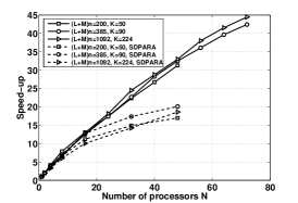
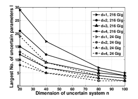
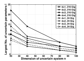
Combining the set-up and SDP components and testing the result of both in cluster computing environments, we demonstrate the capability of robust analysis and control of systems with 100+ states and several uncertain parameters. Specifically, we ran a series of numerical experiments using a local Linux cluster and the Blue Gene supercomputer (with 200 processor allocation). First, we applied the algorithm to a current problem in robust stability analysis of magnetic confinement fusion using a discretized PDE model. Next, we examine the accuracy of the algorithm as Polya’s iterations progress and compare this accuracy with the SOS approach. We show that unlike the general-purpose parallel SDP solver SDPARA [28], the speed-up - the increase in processing speed per additional processor - of our algorithm shows no evidence of saturation. Finally, we calculate the envelope of the algorithm on the Linux cluster in terms of the maximum state-space dimension, number of processors and Polya’s iterations.

NOTATION

We represent llimit-from𝑙l-variate monomials as αγ=i=1lαiγisuperscript𝛼𝛾superscriptsubscriptproduct𝑖1𝑙superscriptsubscript𝛼𝑖subscript𝛾𝑖\alpha^{{\gamma}}=\prod_{i=1}^{l}\alpha_{i}^{\gamma_{i}}, where αl𝛼superscript𝑙\alpha\in\mathbb{R}^{l} is the vector of variables and γl𝛾superscript𝑙\gamma\in\mathbb{N}^{l} is the vector of exponents and i=1lγi=dsuperscriptsubscript𝑖1𝑙subscript𝛾𝑖𝑑\sum_{i=1}^{l}\gamma_{i}=d is the degree of the monomial. We define Wd:={γl:i=1lγi=d}assignsubscript𝑊𝑑conditional-set𝛾superscript𝑙superscriptsubscript𝑖1𝑙subscript𝛾𝑖𝑑W_{d}:=\left\{\gamma\in\mathbb{N}^{l}:\sum_{i=1}^{l}\gamma_{i}=d\right\} as the totally ordered set of the exponents of llimit-from𝑙l-variate monomials of degree d𝑑d, where the ordering is lexicographic. In lexicographical ordering γWd𝛾subscript𝑊𝑑\gamma\in W_{d} precedes ηWd𝜂subscript𝑊𝑑\eta\in W_{d}, if the left most non-zero entry of γη𝛾𝜂\gamma-\eta is positive. The lexicographical index of every γWd𝛾subscript𝑊𝑑\gamma\in W_{d} can be calculated using the map :l:delimited-⟨⟩superscript𝑙\langle{{\cdot}}\rangle:\mathbb{N}^{l}\rightarrow\mathbb{N} defined as [38]

γ=j=1l1i=1γif(lj,d+1k=1j1γki)+1,delimited-⟨⟩𝛾superscriptsubscript𝑗1𝑙1superscriptsubscript𝑖1subscript𝛾𝑖𝑓𝑙𝑗𝑑1superscriptsubscript𝑘1𝑗1subscript𝛾𝑘𝑖1\langle{\gamma}\rangle=\sum_{j=1}^{l-1}\sum_{i=1}^{\gamma_{i}}f\Bigl{(}l-j,d+1-\sum_{k=1}^{j-1}\gamma_{k}-i\Bigr{)}+1, (1)

where as in [39]

f(l,d):={0forl=0(l+d1l1)=(d+l1)!d!(l1)!forl>0,assign𝑓𝑙𝑑cases0for𝑙0binomial𝑙𝑑1𝑙1𝑑𝑙1𝑑𝑙1for𝑙0f(l,d):=\begin{cases}\hskip 14.45377pt0&\text{for}\;\;l=0\\ \dbinom{l+d-1}{l-1}=\dfrac{(d+l-1)!}{d!(l-1)!}&\text{for}\;\;l>0,\end{cases} (2)

is the cardinality of Wdsubscript𝑊𝑑W_{d}, i.e., the number of llimit-from𝑙l-variate monomials of degree d𝑑d. For convenience, we also define the index of a monomial αγsuperscript𝛼𝛾\alpha^{\gamma} to be γdelimited-⟨⟩𝛾\langle\gamma\rangle. We represent llimit-from𝑙l-variate homogeneous polynomials of degree dpsubscript𝑑𝑝d_{p} as

P(α)=γWdpPγαγ,𝑃𝛼subscript𝛾subscript𝑊subscript𝑑𝑝subscript𝑃delimited-⟨⟩𝛾superscript𝛼𝛾P(\alpha)=\sum_{\gamma\in W_{d_{p}}}P_{\langle{\gamma}\rangle}\alpha^{\gamma}, (3)

where Pγn×nsubscript𝑃delimited-⟨⟩𝛾superscript𝑛𝑛P_{\langle{\gamma}\rangle}\in\mathbb{R}^{n\times n} is the matrix coefficient of the monomial αγsuperscript𝛼𝛾\alpha^{\gamma}. We denote the element corresponding to the ithsuperscript𝑖𝑡i^{th} row and jthsuperscript𝑗𝑡j^{th} column of matrix A𝐴A as [A]i,jsubscriptdelimited-[]𝐴𝑖𝑗[A]_{i,j}. The subspace of symmetric matrices in n×nsuperscript𝑛𝑛\mathbb{R}^{n\times n} is denoted by 𝕊nsuperscript𝕊𝑛\mathbb{S}^{n}. We define a basis for 𝕊nsuperscript𝕊𝑛\mathbb{S}^{n} as

[Ek]i,j:={1if i=j=k0otherwise,forknandformulae-sequenceassignsubscriptdelimited-[]subscript𝐸𝑘𝑖𝑗cases1if 𝑖𝑗𝑘0otherwisefor𝑘𝑛and[E_{k}]_{i,j}:=\begin{cases}1&\text{if }i=j=k\\ 0&\text{otherwise}\end{cases},\quad\text{for}\;\,k\leq n\quad\text{and}
[Ek]i,j:=[Fk]i,j+[Fk]i,jT,fork>n,formulae-sequenceassignsubscriptdelimited-[]subscript𝐸𝑘𝑖𝑗subscriptdelimited-[]subscript𝐹𝑘𝑖𝑗subscriptsuperscriptdelimited-[]subscript𝐹𝑘𝑇𝑖𝑗for𝑘𝑛[E_{k}]_{i,j}:=[F_{k}]_{i,j}+[F_{k}]^{T}_{i,j},\quad\text{for}\;\,k>n, (4)

where

[Fk]i,j:={1if i=j1=kn0otherwise.assignsubscriptdelimited-[]subscript𝐹𝑘𝑖𝑗cases1if 𝑖𝑗1𝑘𝑛0otherwise[F_{k}]_{i,j}:=\begin{cases}1&\text{if }i=j-1=k-n\\ 0&\text{otherwise}.\end{cases} (5)

Note that this choice of basis is arbitrary - any other basis could be used. However, any change in basis would require modifications to the formulae defined in this paper. The canonical basis for nsuperscript𝑛\mathbb{R}^{n} is denoted by eisubscript𝑒𝑖e_{i} for i=1,,n𝑖1𝑛i=1,\cdots,n, where ei=[0 01ith0 0].subscript𝑒𝑖delimited-[]0 0superscript1superscript𝑖𝑡0 0e_{i}=[0\>...\>0\overbrace{1}^{i^{th}}0\>...\>0]. The vector with all entries equal to one is denoted by 11\vec{1}. The trace of An×n𝐴superscript𝑛𝑛A\in\mathbb{R}^{n\times n} is denoted by tr(A)=i=1n[A]i,i𝑡𝑟𝐴superscriptsubscript𝑖1𝑛subscriptdelimited-[]𝐴𝑖𝑖tr(A)=\sum_{i=1}^{n}[A]_{i,i}. The block-diagonal matrix with diagonal blocks X1,,Xmn×nsubscript𝑋1subscript𝑋𝑚superscript𝑛𝑛X_{1},\cdots,X_{m}\in\mathbb{R}^{n\times n} is denoted diag(X1,,Xm)mn×mndiagsubscript𝑋1subscript𝑋𝑚superscript𝑚𝑛𝑚𝑛\text{diag}(X_{1},\cdots,X_{m})\in\mathbb{R}^{mn\times mn} or occasionally as diag(Xi|i=1m)mn×mndiagevaluated-atsubscript𝑋𝑖𝑖1𝑚superscript𝑚𝑛𝑚𝑛\text{diag}(X_{i}|_{i=1}^{m})\in\mathbb{R}^{mn\times mn}. The identity and zero matrices are denoted by Inn×nsubscript𝐼𝑛superscript𝑛𝑛I_{n}\in\mathbb{R}^{n\times n} and 0nn×nsubscript0𝑛superscript𝑛𝑛0_{n}\in\mathbb{R}^{n\times n}.

II PRELIMINARIES

Consider the linear system

x˙(t)=A(α)x(t),˙𝑥𝑡𝐴𝛼𝑥𝑡\dot{x}(t)=A(\alpha)x(t), (6)

where A(α)n×n𝐴𝛼superscript𝑛𝑛A(\alpha)\in\mathbb{R}^{n\times n} and αQl𝛼𝑄superscript𝑙\alpha\in Q\subset\mathbb{R}^{l} is a vector of uncertain parameters. In this paper, we consider the case where A(α)𝐴𝛼A(\alpha) is a homogeneous polynomial and Q=Δll𝑄subscriptΔ𝑙superscript𝑙Q=\Delta_{l}\subset\mathbb{R}^{l} where ΔlsubscriptΔ𝑙\Delta_{l} is the unit simplex, i.e.,

Δl={αl,i=1lαi=1,αi0}.subscriptΔ𝑙formulae-sequence𝛼superscript𝑙formulae-sequencesuperscriptsubscript𝑖1𝑙subscript𝛼𝑖1subscript𝛼𝑖0\Delta_{l}=\left\{\alpha\in\mathbb{R}^{l},\sum_{i=1}^{l}\alpha_{i}=1,\alpha_{i}\geqslant 0\right\}. (7)

If A(α)𝐴𝛼A(\alpha) is not homogeneous, we can obtain an equivalent homogeneous representation in the following manner. Suppose A(α)𝐴𝛼A(\alpha) is a non-homogeneous polynomial with αΔl𝛼subscriptΔ𝑙\alpha\in\Delta_{l}, is of degree dasubscript𝑑𝑎d_{a} and has Nasubscript𝑁𝑎N_{a} monomials with non-zero coefficients. Define D=(da1,,daNa)𝐷subscript𝑑subscript𝑎1subscript𝑑subscript𝑎subscript𝑁𝑎D=\left(d_{a_{1}},\cdots,d_{a_{N_{a}}}\right), where daisubscript𝑑subscript𝑎𝑖d_{a_{i}} is the degree of the ithsuperscript𝑖𝑡i^{th} monomial of A(α)𝐴𝛼A(\alpha) according to lexicographical ordering. Now define the polynomial B(α)𝐵𝛼B(\alpha) as per the following.

  1. 1.

    Let B=A𝐵𝐴B=A.

  2. 2.

    For i=1,,Na𝑖1subscript𝑁𝑎i=1,\cdots,N_{a}, multiply the ithsuperscript𝑖𝑡i^{th} monomial of B(α)𝐵𝛼B(\alpha), according to lexicographical ordering, by (j=1lαj)dadaisuperscriptsuperscriptsubscript𝑗1𝑙subscript𝛼𝑗subscript𝑑𝑎subscript𝑑subscript𝑎𝑖\left(\sum_{j=1}^{l}\alpha_{j}\right)^{d_{a}-d_{a_{i}}}.

Then, since j=1lαj=1superscriptsubscript𝑗1𝑙subscript𝛼𝑗1\sum_{j=1}^{l}\alpha_{j}=1, B(α)=A(α)𝐵𝛼𝐴𝛼B(\alpha)=A(\alpha) for all αΔl𝛼subscriptΔ𝑙\alpha\in\Delta_{l} and hence all properties of x˙(t)=A(α)x(t)˙𝑥𝑡𝐴𝛼𝑥𝑡\dot{x}(t)=A(\alpha)x(t) are retained by the homogeneous system x˙(t)=B(α)x(t)˙𝑥𝑡𝐵𝛼𝑥𝑡\dot{x}(t)=B(\alpha)x(t).

1) Example: Construction of the homogeneous system x˙(t)=B(α)x(t)˙𝑥𝑡𝐵𝛼𝑥𝑡\dot{x}(t)=B(\alpha)x(t).

Consider the non-homogeneous polynomial A(α)=Cα12+Dα2+Eα3+F𝐴𝛼𝐶superscriptsubscript𝛼12𝐷subscript𝛼2𝐸subscript𝛼3𝐹A(\alpha)=C\alpha_{1}^{2}+D\alpha_{2}+E\alpha_{3}+F of degree da=2subscript𝑑𝑎2d_{a}=2, where [α1,α2,α3]Δ3subscript𝛼1subscript𝛼2subscript𝛼3subscriptΔ3[\alpha_{1},\alpha_{2},\alpha_{3}]\in\Delta_{3}. Using the above procedure, the homogeneous polynomial B(α)𝐵𝛼B(\alpha) can be constructed as

B(α)=Cα12+Dα2(α1+α2+α3)+Eα3(α1+α2+α3)𝐵𝛼𝐶superscriptsubscript𝛼12𝐷subscript𝛼2subscript𝛼1subscript𝛼2subscript𝛼3𝐸subscript𝛼3subscript𝛼1subscript𝛼2subscript𝛼3\displaystyle B(\alpha)=C\alpha_{1}^{2}+D\alpha_{2}(\alpha_{1}+\alpha_{2}+\alpha_{3})+E\alpha_{3}(\alpha_{1}+\alpha_{2}+\alpha_{3})
+F(α1+α2+α3)2=(C+FB1)α12+(D+2F)B2α1α2𝐹superscriptsubscript𝛼1subscript𝛼2subscript𝛼32subscript𝐶𝐹subscript𝐵1superscriptsubscript𝛼12subscript𝐷2𝐹subscript𝐵2subscript𝛼1subscript𝛼2\displaystyle+F(\alpha_{1}+\alpha_{2}+\alpha_{3})^{2}=(\underbrace{C+F}_{B_{1}})\alpha_{1}^{2}+\underbrace{(D+2F)}_{B_{2}}\alpha_{1}\alpha_{2}
+(E+2F)B3α1α3+(D+F)B4α22+(D+E+2F)B5α2α3subscript𝐸2𝐹subscript𝐵3subscript𝛼1subscript𝛼3subscript𝐷𝐹subscript𝐵4superscriptsubscript𝛼22subscript𝐷𝐸2𝐹subscript𝐵5subscript𝛼2subscript𝛼3\displaystyle+\underbrace{(E+2F)}_{B_{3}}\alpha_{1}\alpha_{3}+\underbrace{(D+F)}_{B_{4}}\alpha_{2}^{2}+\underbrace{(D+E+2F)}_{B_{5}}\alpha_{2}\alpha_{3}
+(E+F)B6α32=γW2Bγαγ.subscript𝐸𝐹subscript𝐵6superscriptsubscript𝛼32subscript𝛾subscript𝑊2subscript𝐵delimited-⟨⟩𝛾superscript𝛼𝛾\displaystyle+\underbrace{(E+F)}_{B_{6}}\alpha_{3}^{2}=\sum_{\gamma\in W_{2}}B_{\langle{\gamma}\rangle}\alpha^{\gamma}. (8)

The following is a stability condition [25] for System (6).

Theorem 1

System (6) is stable if and only if there exists a polynomial matrix P(α)𝑃𝛼P(\alpha) such that P(α)0succeeds𝑃𝛼0P(\alpha)\succ 0 and

AT(α)P(α)+P(α)A(α)0precedessuperscript𝐴𝑇𝛼𝑃𝛼𝑃𝛼𝐴𝛼0A^{T}(\alpha)P(\alpha)+P(\alpha)A(\alpha)\prec 0 (9)

for all αΔl𝛼subscriptΔ𝑙\alpha\in\Delta_{l}.

A similar condition also holds for discrete-time linear systems. The conditions associated with Theorem 1 are infinite-dimensional LMIs, meaning they must hold at infinite number of points. Such problems are known to be NP-hard [17]. In this paper we derive a sequence of polynomial-time algorithms such that their outputs converge to the solution of the infinite-dimensional LMI. Key to this result is Polya’s Theorem [40]. A variation of this theorem for matrices is given as follows.

Theorem 2

(Polya’s Theorem) The homogeneous polynomial F(α)0succeeds𝐹𝛼0F(\alpha)\succ 0 for all αΔl𝛼subscriptΔ𝑙\alpha\in\Delta_{l} if and only if for all sufficiently large d𝑑d,

(i=1lαi)dF(α)superscriptsuperscriptsubscript𝑖1𝑙subscript𝛼𝑖𝑑𝐹𝛼\left(\sum_{i=1}^{l}\alpha_{i}\right)^{d}F(\alpha) (10)

has all positive definite coefficients.

Upper bounds for Polya’s exponent d𝑑d can be found as in [41]. However, these bounds are based on the properties of F𝐹F and are difficult to determine a priori. In this paper, we show that applying Polya’s Theorem to the robust stability problem, i.e., the inequalities in Theorem 1 yields a semi-definite programming condition with an efficiently distributable structure. This is discussed in the following section.

III PROBLEM SET-UP

In this section, we show how Polya’s theorem can be used to determine the robust stability of an uncertain system using linear matrix inequalities with a distributable structure.

III-A Polya’s Algorithm

We consider the stability of the system described by Equation (6). We are interested in finding a P(α)𝑃𝛼P(\alpha) which satisfies the conditions of Theorem 1. According to Polya’s theorem, the constraints of Theorem 1 are satisfied if for some sufficiently large d1subscript𝑑1d_{1} and d2subscript𝑑2d_{2}, the polynomials

(i=1lαi)d1P(α)andsuperscriptsuperscriptsubscript𝑖1𝑙subscript𝛼𝑖subscript𝑑1𝑃𝛼and\left(\sum_{i=1}^{l}\alpha_{i}\right)^{d_{1}}P(\alpha)\qquad\text{and} (11)
(i=1lαi)d2(AT(α)P(α)+P(α)A(α))superscriptsuperscriptsubscript𝑖1𝑙subscript𝛼𝑖subscript𝑑2superscript𝐴𝑇𝛼𝑃𝛼𝑃𝛼𝐴𝛼-\left(\sum_{i=1}^{l}\alpha_{i}\right)^{d_{2}}\left(A^{T}(\alpha)P(\alpha)+P(\alpha)A(\alpha)\right) (12)

have all positive definite coefficients.

Let P(α)𝑃𝛼P(\alpha) be a homogeneous polynomial of degree dpsubscript𝑑𝑝d_{p} which can be represented as

P(α)=γWdpPγαγ,𝑃𝛼subscript𝛾subscript𝑊subscript𝑑𝑝subscript𝑃delimited-⟨⟩𝛾superscript𝛼𝛾P(\alpha)=\sum_{\gamma\in W_{d_{p}}}P_{\langle{\gamma}\rangle}\alpha^{{\gamma}}, (13)

where the coefficients Pγ𝕊nsubscript𝑃delimited-⟨⟩𝛾superscript𝕊𝑛P_{\langle\gamma\rangle}\in\mathbb{S}^{n} and where we recall that Wdp:={γl:i=1lγi=dp}assignsubscript𝑊subscript𝑑𝑝conditional-set𝛾superscript𝑙superscriptsubscript𝑖1𝑙subscript𝛾𝑖subscript𝑑𝑝W_{d_{p}}:=\left\{\gamma\in\mathbb{N}^{l}\,:\,\sum_{i=1}^{l}\gamma_{i}=d_{p}\right\} is the set of the exponents of all l𝑙l-variate monomials of degree dpsubscript𝑑𝑝d_{p}. Since A(α)𝐴𝛼A(\alpha) is a homogeneous polynomial of degree dasubscript𝑑𝑎d_{a}, we can write it as

A(α)=γWdaAγαγ,𝐴𝛼subscript𝛾subscript𝑊subscript𝑑𝑎subscript𝐴delimited-⟨⟩𝛾superscript𝛼𝛾A(\alpha)=\sum_{\gamma\in W_{d_{a}}}A_{\langle{\gamma}\rangle}\alpha^{{\gamma}}, (14)

where the coefficients Aγn×nsubscript𝐴delimited-⟨⟩𝛾superscript𝑛𝑛A_{\langle\gamma\rangle}\in\mathbb{R}^{n\times n}. By substituting (13) and (14) into (11) and (12) and defining dpasubscript𝑑𝑝𝑎d_{pa} as the degree of P(α)A(α)𝑃𝛼𝐴𝛼P(\alpha)A(\alpha), the conditions of Theorem 2 can be represented in the form

hWdpβh,γPh0;γWdp+d1andformulae-sequencesucceedssubscriptsubscript𝑊subscript𝑑𝑝subscript𝛽delimited-⟨⟩delimited-⟨⟩𝛾subscript𝑃delimited-⟨⟩0𝛾subscript𝑊subscript𝑑𝑝subscript𝑑1and\sum_{h\in W_{d_{p}}}\beta_{\langle{h}\rangle,\langle{\gamma}\rangle}P_{\langle{h}\rangle}\succ 0;\quad\gamma\in W_{d_{p}+d_{1}}\;\text{and} (15)
hWdp(Hh,γTPh+PhHh,γ)0;γWdpa+d2.formulae-sequenceprecedessubscriptsubscript𝑊subscript𝑑𝑝superscriptsubscript𝐻delimited-⟨⟩delimited-⟨⟩𝛾𝑇subscript𝑃delimited-⟨⟩subscript𝑃delimited-⟨⟩subscript𝐻delimited-⟨⟩delimited-⟨⟩𝛾0𝛾subscript𝑊subscript𝑑𝑝𝑎subscript𝑑2\sum_{h\in W_{d_{p}}}(H_{\langle{h}\rangle,\langle{\gamma}\rangle}^{T}P_{\langle{h}\rangle}+P_{\langle{h}\rangle}H_{\langle{h}\rangle,\langle{\gamma}\rangle})\prec 0;\;\gamma\in W_{d_{pa}+d_{2}}. (16)

Here βh,γsubscript𝛽delimited-⟨⟩delimited-⟨⟩𝛾\beta_{\langle{h}\rangle,\langle{\gamma}\rangle} is defined to be the scalar coefficient which multiplies Phsubscript𝑃delimited-⟨⟩P_{\langle{h}\rangle} in the γdelimited-⟨⟩𝛾\langle{\gamma}\rangle-th monomial of the homogeneous polynomial (i=1lαi)d1P(α)superscriptsuperscriptsubscript𝑖1𝑙subscript𝛼𝑖subscript𝑑1𝑃𝛼\left(\sum_{i=1}^{l}\alpha_{i}\right)^{d_{1}}P(\alpha) using the lexicographical ordering. Likewise Hh,γn×nsubscript𝐻delimited-⟨⟩delimited-⟨⟩𝛾superscript𝑛𝑛H_{\langle{h}\rangle,\langle{\gamma}\rangle}\in\mathbb{R}^{n\times n} is the term which left or right multiplies Phsubscript𝑃delimited-⟨⟩P_{\langle{h}\rangle} in the γdelimited-⟨⟩𝛾\langle{\gamma}\rangle-th monomial of (i=1lαi)d2(AT(α)P(α)+P(α)A(α))superscriptsuperscriptsubscript𝑖1𝑙subscript𝛼𝑖subscript𝑑2superscript𝐴𝑇𝛼𝑃𝛼𝑃𝛼𝐴𝛼\left(\sum_{i=1}^{l}\alpha_{i}\right)^{d_{2}}\left(A^{T}(\alpha)P(\alpha)+P(\alpha)A(\alpha)\right) using the lexicographical ordering. For an intuitive explanation as to how these β𝛽\beta and H𝐻H terms are calculated, we consider a simple example. Precise formulae for these terms will follow the example.

1) Example: Calculating the β𝛽\beta and H𝐻H coefficients.

Consider A(α)=A1α1+A2α2𝐴𝛼subscript𝐴1subscript𝛼1subscript𝐴2subscript𝛼2A(\alpha)=A_{1}\alpha_{1}+A_{2}\alpha_{2} and P(α)=P1α1+P2α2𝑃𝛼subscript𝑃1subscript𝛼1subscript𝑃2subscript𝛼2P(\alpha)=P_{1}\alpha_{1}+P_{2}\alpha_{2}. By expanding Equation (11) for d1=1subscript𝑑11d_{1}=1 we have

(α1+α2)P(α)=P1α12+(P1+P2)α1α2+P2α22.subscript𝛼1subscript𝛼2𝑃𝛼subscript𝑃1superscriptsubscript𝛼12subscript𝑃1subscript𝑃2subscript𝛼1subscript𝛼2subscript𝑃2superscriptsubscript𝛼22(\alpha_{1}+\alpha_{2})P(\alpha)=P_{1}\alpha_{1}^{2}+(P_{1}+P_{2})\alpha_{1}\alpha_{2}+P_{2}\alpha_{2}^{2}. (17)

The βh,γsubscript𝛽delimited-⟨⟩delimited-⟨⟩𝛾\beta_{\langle{h}\rangle,\langle{\gamma}\rangle} terms are then extracted as

β1,1=1,β2,1=0,β1,2=1,β2,2=1,β1,3=0,β2,3=1.formulae-sequencesubscript𝛽111formulae-sequencesubscript𝛽210formulae-sequencesubscript𝛽121formulae-sequencesubscript𝛽221formulae-sequencesubscript𝛽130subscript𝛽231\beta_{1,1}=1,\;\beta_{2,1}=0,\;\beta_{1,2}=1,\;\beta_{2,2}=1,\;\beta_{1,3}=0,\;\beta_{2,3}=1. (18)

Next, by expanding Equation (12) for d2=1subscript𝑑21d_{2}=1 we have

(α1+α2)(AT(α)P(α)+P(α)A(α))=(A1TP1+P1A1)α13subscript𝛼1subscript𝛼2superscript𝐴𝑇𝛼𝑃𝛼𝑃𝛼𝐴𝛼subscriptsuperscript𝐴𝑇1subscript𝑃1subscript𝑃1subscript𝐴1superscriptsubscript𝛼13\displaystyle(\alpha_{1}+\alpha_{2})\left(A^{T}(\alpha)P(\alpha)+P(\alpha)A(\alpha)\right)=\left(A^{T}_{1}P_{1}+P_{1}A_{1}\right)\alpha_{1}^{3}
+(A1TP1+P1A1+A2TP1+P1A2+A1TP2+P2A1)α12α2subscriptsuperscript𝐴𝑇1subscript𝑃1subscript𝑃1subscript𝐴1subscriptsuperscript𝐴𝑇2subscript𝑃1subscript𝑃1subscript𝐴2subscriptsuperscript𝐴𝑇1subscript𝑃2subscript𝑃2subscript𝐴1superscriptsubscript𝛼12subscript𝛼2\displaystyle+\left(A^{T}_{1}P_{1}+P_{1}A_{1}+A^{T}_{2}P_{1}+P_{1}A_{2}+A^{T}_{1}P_{2}+P_{2}A_{1}\right)\alpha_{1}^{2}\alpha_{2}
+(A2TP1+P1A2+A1TP2+P2A1+A2TP2+P2A2)α1α22subscriptsuperscript𝐴𝑇2subscript𝑃1subscript𝑃1subscript𝐴2subscriptsuperscript𝐴𝑇1subscript𝑃2subscript𝑃2subscript𝐴1subscriptsuperscript𝐴𝑇2subscript𝑃2subscript𝑃2subscript𝐴2subscript𝛼1superscriptsubscript𝛼22\displaystyle+\left(A^{T}_{2}P_{1}+P_{1}A_{2}+A^{T}_{1}P_{2}+P_{2}A_{1}+A^{T}_{2}P_{2}+P_{2}A_{2}\right)\alpha_{1}\alpha_{2}^{2}
+(A2TP2+P2A2)α23.subscriptsuperscript𝐴𝑇2subscript𝑃2subscript𝑃2subscript𝐴2superscriptsubscript𝛼23\displaystyle+\left(A^{T}_{2}P_{2}+P_{2}A_{2}\right)\alpha_{2}^{3}. (19)

The Hh,γsubscript𝐻delimited-⟨⟩delimited-⟨⟩𝛾H_{\langle{h}\rangle,\langle{\gamma}\rangle} terms are then extracted as

H1,1=A1,subscript𝐻11subscript𝐴1\displaystyle H_{1,1}=A_{1}, H2,1=0,subscript𝐻210\displaystyle H_{2,1}=\textbf{0}, H1,2=A1+A2,subscript𝐻12subscript𝐴1subscript𝐴2\displaystyle H_{1,2}=A_{1}+A_{2}, H2,2=A1,subscript𝐻22subscript𝐴1\displaystyle H_{2,2}=A_{1},
H1,3=A2,subscript𝐻13subscript𝐴2\displaystyle H_{1,3}=A_{2}, H2,3=A1+A2,subscript𝐻23subscript𝐴1subscript𝐴2\displaystyle H_{2,3}=A_{1}+A_{2}, H1,4=0,subscript𝐻140\displaystyle H_{1,4}=\textbf{0}, H2,4=A2.subscript𝐻24subscript𝐴2\displaystyle H_{2,4}=A_{2}. (20)

2) General Formula: The {βh,γ}subscript𝛽delimited-⟨⟩delimited-⟨⟩𝛾\{\beta_{\langle{h}\rangle,\langle{\gamma}\rangle}\} can be formally defined recursively as follows. Let the initial values for βh,γsubscript𝛽delimited-⟨⟩delimited-⟨⟩𝛾\beta_{\langle{h}\rangle,\langle{\gamma}\rangle} be defined as

βh,γ(0)={1if h=γ0otherwiseforγWdpandhWdp.formulae-sequencesubscriptsuperscript𝛽0delimited-⟨⟩delimited-⟨⟩𝛾cases1if 𝛾0otherwisefor𝛾subscript𝑊subscript𝑑𝑝andsubscript𝑊subscript𝑑𝑝\beta^{(0)}_{\langle{h}\rangle,\langle{\gamma}\rangle}=\begin{cases}1&\text{if }h=\gamma\\ 0&\text{otherwise}\end{cases}\qquad\text{for}\;\gamma\in W_{d_{p}}\;\text{and}\;h\in W_{d_{p}}. (21)

Then, iterating for i=1,d1𝑖1subscript𝑑1i=1,\ldots d_{1}, we let

βh,γ(i)=λW1βh,γλ(i1)forγWdp+iandhWdp.formulae-sequencesubscriptsuperscript𝛽𝑖delimited-⟨⟩delimited-⟨⟩𝛾subscript𝜆subscript𝑊1subscriptsuperscript𝛽𝑖1delimited-⟨⟩delimited-⟨⟩𝛾𝜆for𝛾subscript𝑊subscript𝑑𝑝𝑖andsubscript𝑊subscript𝑑𝑝\beta^{(i)}_{\langle{h}\rangle,\langle{\gamma}\rangle}=\sum_{\lambda\in W_{1}}\beta^{(i-1)}_{\langle{h}\rangle,\langle{\gamma-\lambda}\rangle}\qquad\text{for}\;\gamma\in W_{d_{p}+i}\;\text{and}\;h\in W_{d_{p}}. (22)

Finally, we set {βh,γ}={βh,γd1}subscript𝛽delimited-⟨⟩delimited-⟨⟩𝛾subscriptsuperscript𝛽subscript𝑑1delimited-⟨⟩delimited-⟨⟩𝛾\{\beta_{\langle{h}\rangle,\langle{\gamma}\rangle}\}=\{\beta^{d_{1}}_{\langle{h}\rangle,\langle{\gamma}\rangle}\}. To obtain {Hh,γ}subscript𝐻delimited-⟨⟩delimited-⟨⟩𝛾\{{H_{\langle{h}\rangle,\langle{\gamma}\rangle}}\}, set the initial values as

Hh,γ(0)=λWda:λ+h=γAλforγWdp+daandhWdp.subscriptsuperscript𝐻0delimited-⟨⟩delimited-⟨⟩𝛾subscript:𝜆subscript𝑊subscript𝑑𝑎𝜆𝛾subscript𝐴delimited-⟨⟩𝜆for𝛾subscript𝑊subscript𝑑𝑝subscript𝑑𝑎andsubscript𝑊subscript𝑑𝑝H^{(0)}_{\langle{h}\rangle,\langle{\gamma}\rangle}=\sum_{\lambda\in W_{d_{a}}:\lambda+h=\gamma}A_{\langle{\lambda}\rangle}\;\;\text{for}\;\gamma\in W_{d_{p}+d_{a}}\;\text{and}\;h\in W_{d_{p}}. (23)

Then, iterating for i=1,d2𝑖1subscript𝑑2i=1,\ldots d_{2}, we let

Hh,γ(i)=λW1Hh,γλ(i1)forγWdpa+iandhWdp.formulae-sequencesubscriptsuperscript𝐻𝑖delimited-⟨⟩delimited-⟨⟩𝛾subscript𝜆subscript𝑊1subscriptsuperscript𝐻𝑖1delimited-⟨⟩delimited-⟨⟩𝛾𝜆for𝛾subscript𝑊subscript𝑑𝑝𝑎𝑖andsubscript𝑊subscript𝑑𝑝H^{(i)}_{\langle{h}\rangle,\langle{\gamma}\rangle}=\sum_{\lambda\in W_{1}}H^{(i-1)}_{\langle{h}\rangle,\langle{\gamma-\lambda}\rangle}\quad\text{for}\;\gamma\in W_{d_{pa}+i}\;\text{and}\;h\in W_{d_{p}}. (24)

Finally, set {Hh,γ}={Hh,γd2}subscript𝐻delimited-⟨⟩delimited-⟨⟩𝛾subscriptsuperscript𝐻subscript𝑑2delimited-⟨⟩delimited-⟨⟩𝛾\{H_{\langle{h}\rangle,\langle{\gamma}\rangle}\}=\{H^{d_{2}}_{\langle{h}\rangle,\langle{\gamma}\rangle}\}.

Refer to caption
Refer to caption
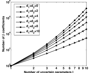
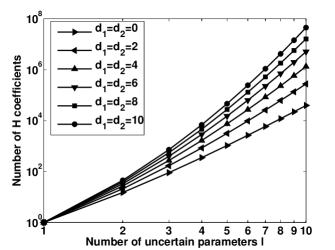
Figure 1: Number of βh,γsubscript𝛽delimited-⟨⟩delimited-⟨⟩𝛾\beta_{\langle{h}\rangle,\langle{\gamma}\rangle} and Hh,γsubscript𝐻delimited-⟨⟩delimited-⟨⟩𝛾H_{\langle{h}\rangle,\langle{\gamma}\rangle} coefficients vs. the number of uncertain parameters for different Polya’s exponents and for dp=da=2subscript𝑑𝑝subscript𝑑𝑎2d_{p}=d_{a}=2

For the case of large-scale systems, computing and storing {βh,γ}subscript𝛽delimited-⟨⟩delimited-⟨⟩𝛾\{\beta_{\langle{h}\rangle,\langle{\gamma}\rangle}\} and {Hh,γ}subscript𝐻delimited-⟨⟩delimited-⟨⟩𝛾\{{H_{\langle{h}\rangle,\langle{\gamma}\rangle}}\} is a significant challenge due to the number of these coefficients. Specifically, the number of terms increases with l𝑙l (number of uncertain parameters in system (6)), dpsubscript𝑑𝑝d_{p} (degree of P(α)𝑃𝛼P(\alpha)), dpasubscript𝑑𝑝𝑎d_{pa} (degree of P(α)A(α)𝑃𝛼𝐴𝛼P(\alpha)A(\alpha)) and d1,d2subscript𝑑1subscript𝑑2d_{1},d_{2} (Polya’s exponents) as follows.

3) Number of βh,γsubscript𝛽delimited-⟨⟩delimited-⟨⟩𝛾\beta_{\langle{h}\rangle,\langle{\gamma}\rangle} coefficients: For given l,dp𝑙subscript𝑑𝑝l,d_{p} and d1subscript𝑑1d_{1}, since hWdpsubscript𝑊subscript𝑑𝑝h\in W_{d_{p}} and γWdp+d1𝛾subscript𝑊subscript𝑑𝑝subscript𝑑1\gamma\in W_{d_{p}+d_{1}}, the number of βh,γsubscript𝛽delimited-⟨⟩delimited-⟨⟩𝛾\beta_{\langle{h}\rangle,\langle{\gamma}\rangle} coefficients is the product of L0:=card(Wdp)assignsubscript𝐿0cardsubscript𝑊subscript𝑑𝑝L_{0}:=\text{card}(W_{d_{p}}) and L:=card(Wdp+d1)assign𝐿cardsubscript𝑊subscript𝑑𝑝subscript𝑑1L:=\text{card}(W_{d_{p}+d_{1}}). Recall that card(Wdp)subscript𝑊subscript𝑑𝑝(W_{d_{p}}) is the number of all l𝑙l-variate monomials of degree dpsubscript𝑑𝑝d_{p} and can be calculated using (2) as follows.

L0=f(l,dp)={0forl=0(dp+l1l1)=(dp+l1)!dp!(l1)!forl>0.subscript𝐿0𝑓𝑙subscript𝑑𝑝cases0for𝑙0binomialsubscript𝑑𝑝𝑙1𝑙1subscript𝑑𝑝𝑙1subscript𝑑𝑝𝑙1for𝑙0L_{0}=f(l,d_{p})=\begin{cases}\hskip 14.45377pt0&\text{for}\;\;l=0\\ \dbinom{d_{p}+l-1}{l-1}=\dfrac{(d_{p}+l-1)!}{d_{p}!(l-1)!}&\text{for}\;\;l>0.\end{cases} (25)

Likewise, card(Wdp+d1)subscript𝑊subscript𝑑𝑝subscript𝑑1(W_{d_{p}+d_{1}}), i.e., the number of all llimit-from𝑙l-variate monomials of degree dp+d1subscript𝑑𝑝subscript𝑑1d_{p}+d_{1} is calculated using (2) as follows.

L=f(l,dp+d1)=𝐿𝑓𝑙subscript𝑑𝑝subscript𝑑1absent\displaystyle L=f(l,d_{p}+d_{1})=
{0forl=0(dp+d1+l1l1)=(dp+d1+l1)!(dp+d1)!(l1)!forl>0.cases0for𝑙0binomialsubscript𝑑𝑝subscript𝑑1𝑙1𝑙1subscript𝑑𝑝subscript𝑑1𝑙1subscript𝑑𝑝subscript𝑑1𝑙1for𝑙0\displaystyle\begin{cases}\hskip 14.45377pt0&\text{for}\;\;l=0\\ \dbinom{d_{p}+d_{1}+l-1}{l-1}=\dfrac{(d_{p}+d_{1}+l-1)!}{(d_{p}+d_{1})!(l-1)!}&\text{for}\;\;l>0.\end{cases} (26)

The number of βh,γsubscript𝛽delimited-⟨⟩delimited-⟨⟩𝛾\beta_{\langle{h}\rangle,\langle{\gamma}\rangle} coefficients is L0Lsubscript𝐿0𝐿L_{0}\cdot L.

4) Number of Hh,γsubscript𝐻delimited-⟨⟩delimited-⟨⟩𝛾H_{\langle{h}\rangle,\langle{\gamma}\rangle} coefficients: For given l,dp,da𝑙subscript𝑑𝑝subscript𝑑𝑎l,d_{p},d_{a} and d2subscript𝑑2d_{2}, since hWdpsubscript𝑊subscript𝑑𝑝h\in W_{d_{p}} and γWdpa+d2𝛾subscript𝑊subscript𝑑𝑝𝑎subscript𝑑2\gamma\in W_{d_{pa}+d_{2}}, the number of Hh,γsubscript𝐻delimited-⟨⟩delimited-⟨⟩𝛾H_{\langle{h}\rangle,\langle{\gamma}\rangle} coefficients is the product of L0:=card(Wdp)assignsubscript𝐿0cardsubscript𝑊subscript𝑑𝑝L_{0}:=\text{card}(W_{d_{p}}) and M:=card(Wdpa+d2)assign𝑀cardsubscript𝑊subscript𝑑𝑝𝑎subscript𝑑2M:=\text{card}(W_{d_{pa}+d_{2}}). By using (2), we have

M=f(l,dpa+d2)=𝑀𝑓𝑙subscript𝑑𝑝𝑎subscript𝑑2absent\displaystyle M=f(l,d_{pa}+d_{2})=
{0forl=0(dpa+d2+l1l1)=(dpa+d2+l1)!(dpa+d2)!(l1)!forl>0.cases0for𝑙0binomialsubscript𝑑𝑝𝑎subscript𝑑2𝑙1𝑙1subscript𝑑𝑝𝑎subscript𝑑2𝑙1subscript𝑑𝑝𝑎subscript𝑑2𝑙1for𝑙0\displaystyle\begin{cases}\hskip 14.45377pt0&\text{for}\;\;l=0\\ \dbinom{d_{pa}+d_{2}+l-1}{l-1}=\dfrac{(d_{pa}+d_{2}+l-1)!}{(d_{pa}+d_{2})!(l-1)!}&\text{for}\;\;l>0.\end{cases} (27)

The number of Hh,γsubscript𝐻delimited-⟨⟩delimited-⟨⟩𝛾H_{\langle{h}\rangle,\langle{\gamma}\rangle} coefficients is L0Msubscript𝐿0𝑀L_{0}\cdot M.

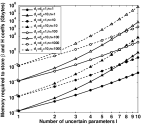
The number of βh,γsubscript𝛽delimited-⟨⟩delimited-⟨⟩𝛾\beta_{\langle{h}\rangle,\langle{\gamma}\rangle} and Hh,γsubscript𝐻delimited-⟨⟩delimited-⟨⟩𝛾H_{\langle{h}\rangle,\langle{\gamma}\rangle} coefficients and the required memory to store these coefficients are shown in Figs. 1 and 2 in terms of the number of uncertain parameters l𝑙l and for different Polya’s exponents. In all cases dp=da=2subscript𝑑𝑝subscript𝑑𝑎2d_{p}=d_{a}=2.

Refer to caption
Figure 2: Memory required to store β𝛽\beta and H𝐻H coefficients vs. number of uncertain parameters, for different d1,d2subscript𝑑1subscript𝑑2d_{1},d_{2} and dp=da=2subscript𝑑𝑝subscript𝑑𝑎2d_{p}=d_{a}=2

It is observed from Fig. 2 that, even for small dpsubscript𝑑𝑝d_{p} and dasubscript𝑑𝑎d_{a}, the required memory is in the Terabyte range. In [38], we proposed a decentralized computing approach to the calculation of {βh,γ}subscript𝛽delimited-⟨⟩delimited-⟨⟩𝛾\{\beta_{\langle{h}\rangle,\langle{\gamma}\rangle}\} on large cluster computers. In the present work, we extend this method to the calculation of {Hh,γ}subscript𝐻delimited-⟨⟩delimited-⟨⟩𝛾\{H_{\langle{h}\rangle,\langle{\gamma}\rangle}\} and the SDP elements which will be discussed in the following section. We express the LMIs associated with conditions (15) and (16) as an SDP in both primal and dual forms. We also discuss the structure of the primal and dual SDP variables and the constraints.

III-B SDP Problem Elements

A semi-definite programming problem can be stated either in primal or dual format. Given C𝕊m𝐶superscript𝕊𝑚C\in\mathbb{S}^{m}, aK𝑎superscript𝐾a\in\mathbb{R}^{K} and Bi𝕊msubscript𝐵𝑖superscript𝕊𝑚B_{i}\in\mathbb{S}^{m}, the primal problem is of the form

maxXtr(CX)subscript𝑋𝑡𝑟𝐶𝑋\max_{X}\quad tr(CX)
subject toaB(X)=0subject to𝑎𝐵𝑋0\hskip 7.22743pt\text{subject to}\quad a-B(X)=0
X0,succeeds-or-equals𝑋0\hskip 25.29494ptX\succeq 0, (28)

where the linear operator B:𝕊mK:𝐵superscript𝕊𝑚superscript𝐾B:\mathbb{S}^{m}\rightarrow\mathbb{R}^{K} is defined as

B(X)=[tr(B1X)tr(B2X)tr(BKX)]T.𝐵𝑋superscriptdelimited-[]𝑡𝑟subscript𝐵1𝑋𝑡𝑟subscript𝐵2𝑋𝑡𝑟subscript𝐵𝐾𝑋missing-subexpressionmissing-subexpression𝑇B(X)=\left[\begin{array}[]{ccc}tr(B_{1}X)\quad tr(B_{2}X)\quad\cdots\quad tr(B_{K}X)\end{array}\right]^{T}. (29)

X𝕊m𝑋superscript𝕊𝑚X\in\mathbb{S}^{m} is the primal variable. Given a primal SDP, the associated dual problem is

miny,ZaTysubscript𝑦𝑍superscript𝑎𝑇𝑦\min_{y,Z}\quad a^{T}y
subject toBT(y)C=Zsubject tosuperscript𝐵𝑇𝑦𝐶𝑍\hskip 14.45377pt\text{subject to}\quad B^{T}(y)-C=Z
Z0,yK,formulae-sequencesucceeds-or-equals𝑍0𝑦superscript𝐾\hskip 72.26999ptZ\succeq 0\;,\;y\in\mathbb{R}^{K}, (30)

where BT:K𝕊m:superscript𝐵𝑇superscript𝐾superscript𝕊𝑚B^{T}:\mathbb{R}^{K}\rightarrow\mathbb{S}^{m} is the transpose operator and is given by

BT(y)=i=1KyiBisuperscript𝐵𝑇𝑦superscriptsubscript𝑖1𝐾subscript𝑦𝑖subscript𝐵𝑖B^{T}(y)=\sum_{i=1}^{K}y_{i}B_{i} (31)

and where yK𝑦superscript𝐾y\in\mathbb{R}^{K} and Z𝕊m𝑍superscript𝕊𝑚Z\in\mathbb{S}^{m} are the dual variables. The elements C𝐶C, Bisubscript𝐵𝑖B_{i} and a𝑎a of the SDP problem associated with the LMIs in (15) and (16) are defined as follows. We define the element C𝐶C as

C:=diag(C1,CL,CL+1,CL+M),assign𝐶diagsubscript𝐶1subscript𝐶𝐿subscript𝐶𝐿1subscript𝐶𝐿𝑀C:=\text{diag}(C_{1},\cdots C_{L},C_{L+1},\cdots C_{L+M}), (32)

where

Ci:={δIn(hWdpβh,idp!h1!hl!),1iL0n,L+1iL+M,assignsubscript𝐶𝑖cases𝛿subscript𝐼𝑛subscriptsubscript𝑊subscript𝑑𝑝subscript𝛽delimited-⟨⟩𝑖subscript𝑑𝑝subscript1subscript𝑙1𝑖𝐿subscript0𝑛𝐿1𝑖𝐿𝑀C_{i}:=\begin{cases}\delta I_{n}\cdot\left(\sum_{h\in W_{d_{p}}}\beta_{\langle h\rangle,i}\,\frac{d_{p}!}{h_{1}!\,\cdots\,h_{l}!}\right),&\hskip 25.29494pt1\leq i\leq L\\ 0_{n},&L+1\leq i\leq L+M,\end{cases} (33)

where recall that L=card(Wdp+d1)𝐿cardsubscript𝑊subscript𝑑𝑝subscript𝑑1L=\text{card}(W_{d_{p}+d_{1}}) is the number of monomials in (i=1lαi)d1P(α)superscriptsuperscriptsubscript𝑖1𝑙subscript𝛼𝑖subscript𝑑1𝑃𝛼\left(\sum_{i=1}^{l}\alpha_{i}\right)^{d_{1}}P(\alpha), M=card(Wdpa+d2)𝑀cardsubscript𝑊subscript𝑑𝑝𝑎subscript𝑑2M=\text{card}(W_{d_{pa}+d_{2}}) is the number of monomials in (i=1lαi)d2P(α)A(α)superscriptsuperscriptsubscript𝑖1𝑙subscript𝛼𝑖subscript𝑑2𝑃𝛼𝐴𝛼\left(\sum_{i=1}^{l}\alpha_{i}\right)^{d_{2}}P(\alpha)A(\alpha), where n𝑛n is the dimension of system (6), l𝑙l is the number of uncertain parameters and δ𝛿\delta is a small positive parameter.

For i=1,,K𝑖1𝐾i=1,\cdots,K, define Bisubscript𝐵𝑖B_{i} elements as

Bi:=diag(Bi,1,Bi,L,Bi,L+1,Bi,L+M),assignsubscript𝐵𝑖diagsubscript𝐵𝑖1subscript𝐵𝑖𝐿subscript𝐵𝑖𝐿1subscript𝐵𝑖𝐿𝑀B_{i}:=\text{diag}(B_{i,1},\cdots B_{i,L},B_{i,L+1},\cdots B_{i,L+M}), (34)

where K𝐾K is the number of dual variables in (30) and is equal to the product of the number of upper-triangular elements in each Pγ𝕊nsubscript𝑃𝛾superscript𝕊𝑛P_{\gamma}\in\mathbb{S}^{n} (the coefficients in P(α)𝑃𝛼P(\alpha)) and the number of coefficients in P(α)𝑃𝛼P(\alpha) (i.e. the cardinality of Wdpsubscript𝑊subscript𝑑𝑝W_{d_{p}}). Since there are f(l,dp)=(dp+l1l1)𝑓𝑙subscript𝑑𝑝binomialsubscript𝑑𝑝𝑙1𝑙1f(l,d_{p})=\dbinom{d_{p}+l-1}{l-1} coefficients in P(α)𝑃𝛼P(\alpha) and each coefficient has N~:=12n(n+1)assign~𝑁12𝑛𝑛1\tilde{N}:=\frac{1}{2}n(n+1) upper-triangular elements, we find

K=(dp+l1)!dp!(l1)!N~.𝐾subscript𝑑𝑝𝑙1subscript𝑑𝑝𝑙1~𝑁K=\frac{(d_{p}+l-1)!}{d_{p}!(l-1)!}\tilde{N}. (35)

To define the Bi,jsubscript𝐵𝑖𝑗B_{i,j} blocks, first we define the function Vh:Kn×n:subscript𝑉delimited-⟨⟩superscript𝐾superscript𝑛𝑛V_{\langle h\rangle}:\mathbb{Z}^{K}\rightarrow\mathbb{Z}^{n\times n},

Vh(x):=j=1N~Ejxj+N~(h1)for allhWdp,formulae-sequenceassignsubscript𝑉delimited-⟨⟩𝑥superscriptsubscript𝑗1~𝑁subscript𝐸𝑗subscript𝑥𝑗~𝑁delimited-⟨⟩1for allsubscript𝑊subscript𝑑𝑝V_{\langle h\rangle}(x):=\sum_{j=1}^{\tilde{N}}E_{j}\;x_{j+\tilde{N}(\langle h\rangle-1)}\quad\text{for all}\quad h\in W_{d_{p}}, (36)

which maps each variable to a basis matrix Ejsubscript𝐸𝑗E_{j}, where recall that Ejsubscript𝐸𝑗E_{j} is the basis for 𝕊nsuperscript𝕊𝑛\mathbb{S}^{n}. Note that a different choice of basis would require a different function Vhsubscript𝑉delimited-⟨⟩V_{\langle h\rangle}. Then for i=1,,K𝑖1𝐾i=1,\cdots,K,

Bi,j:=assignsubscript𝐵𝑖𝑗absent\displaystyle B_{i,j}:=
{hWdpβh,jVh(ei),1jL(I)hWdp(Hh,jLTVh(ei)+Vh(ei)Hh,jL),L+1jL+M.(II)\displaystyle\begin{cases}\sum_{h\in W_{d_{p}}}\beta_{\langle h\rangle,j}V_{\langle h\rangle}(e_{i}),\hskip 72.26999pt1\leq j\leq L\;(I)\\ -\sum_{h\in W_{d_{p}}}\Big{(}H_{{\langle h\rangle},j-L}^{T}V_{\langle h\rangle}(e_{i})+\\ \hskip 43.36243ptV_{\langle h\rangle}(e_{i})H_{{\langle h\rangle},j-L}\Big{)},\;\;L+1\leq j\leq L+M.\;(II)\end{cases} (37)

Finally, to complete the SDP problem associated with Polya’s algorithm set

a=1K.𝑎1superscript𝐾a=\vec{1}\in\mathbb{R}^{K}. (38)

III-C Parallel Set-up Algorithm

In this section, we propose a decentralized, iterative algorithm for calculating the terms {βh,γ}subscript𝛽delimited-⟨⟩delimited-⟨⟩𝛾\{\beta_{\langle h\rangle,\langle\gamma\rangle}\}, {Hh,γ}subscript𝐻delimited-⟨⟩delimited-⟨⟩𝛾\{H_{\langle h\rangle,\langle\gamma\rangle}\}, C𝐶C and Bisubscript𝐵𝑖B_{i} as defined in (22), (24), (32) and (34). The algorithm has been implemented in C++, using MPI (Message Passing Interface) and is available at: www.sites.google.com/a/asu.edu/kamyar/software. We present an abridged description of this algorithm in Algorithm 1, wherein N𝑁N is the number of available processors.

Inputs: dpsubscript𝑑𝑝d_{p}: degree of P(α)𝑃𝛼P(\alpha), dasubscript𝑑𝑎d_{a}: degree of A(α)𝐴𝛼A(\alpha), n𝑛n: number of states, l𝑙l: number of uncertain parameters, d1,d2subscript𝑑1subscript𝑑2d_{1},d_{2}: number of Polya’s iterations, Coefficients of A(α)𝐴𝛼A(\alpha).
Initialization: Set d^1=d^2=0subscript^𝑑1subscript^𝑑20\hat{d}_{1}=\hat{d}_{2}=0 and dpa=dp+dasubscript𝑑𝑝𝑎subscript𝑑𝑝subscript𝑑𝑎d_{pa}=d_{p}+d_{a}. Calculate L0subscript𝐿0L_{0} as the number of monomials in P(α)𝑃𝛼P(\alpha) using (25) and M𝑀M as the number of monomials in P(α)A(α)𝑃𝛼𝐴𝛼P(\alpha)A(\alpha) using (27). Set L=L0𝐿subscript𝐿0L=L_{0}. Calculate L=𝚏𝚕𝚘𝚘𝚛(LN)superscript𝐿𝚏𝚕𝚘𝚘𝚛𝐿𝑁L^{\prime}=\mathtt{floor}(\frac{L}{N}) and M=𝚏𝚕𝚘𝚘𝚛(MN)superscript𝑀𝚏𝚕𝚘𝚘𝚛𝑀𝑁M^{\prime}=\mathtt{floor}(\frac{M}{N}) as the number of monomials in P(α)𝑃𝛼P(\alpha) and P(α)A(α)𝑃𝛼𝐴𝛼P(\alpha)A(\alpha) assigned to each processor.
for i=1,,N𝑖1𝑁i=1,\cdots,N, processor i𝑖i do
       Initialize βk,jsubscript𝛽𝑘𝑗\beta_{k,j} for j=(i1)L+1,,iL𝑗𝑖1superscript𝐿1𝑖superscript𝐿j=(i-1)L^{\prime}+1,\cdots,iL^{\prime} and k=1,L0𝑘1subscript𝐿0k=1,\cdots L_{0} using (21).
       Initialize Hk,msubscript𝐻𝑘𝑚H_{k,m} for m=(i1)M+1,,iM𝑚𝑖1superscript𝑀1𝑖superscript𝑀m=(i-1)M^{\prime}+1,\cdots,iM^{\prime} and k=1,L0𝑘1subscript𝐿0k=1,\cdots L_{0} using (23).
Calculating ββ\beta and HHH coefficients:
while d^1d1subscript^𝑑1subscript𝑑1\hat{d}_{1}\leq d_{1} or d^2d2subscript^𝑑2subscript𝑑2\hat{d}_{2}\leq d_{2} do
       if d^1d1subscript^𝑑1subscript𝑑1\hat{d}_{1}\leq d_{1} then
             for i=1,,N𝑖1𝑁i=1,\cdots,N, processor i𝑖i do
                   Set dp=dp+1subscript𝑑𝑝subscript𝑑𝑝1d_{p}=d_{p}+1 and d^1=d^1+1subscript^𝑑1subscript^𝑑11\hat{d}_{1}=\hat{d}_{1}+1. Update L𝐿L using (26). Update L=𝚏𝚕𝚘𝚘𝚛(LN)superscript𝐿𝚏𝚕𝚘𝚘𝚛𝐿𝑁L^{\prime}=\mathtt{floor}(\frac{L}{N}).
                   Calculate βk,jsubscript𝛽𝑘𝑗\beta_{k,j} for j=(i1)L+1,,iL𝑗𝑖1superscript𝐿1𝑖superscript𝐿j=(i-1)L^{\prime}+1,\cdots,iL^{\prime} and k=1,L0𝑘1subscript𝐿0k=1,\cdots L_{0} using (22).
            
      if d^2d2subscript^𝑑2subscript𝑑2\hat{d}_{2}\leq d_{2} then
             for i=1,,N𝑖1𝑁i=1,\cdots,N, processor i𝑖i do
                   Set dpa=dpa+1subscript𝑑𝑝𝑎subscript𝑑𝑝𝑎1d_{pa}=d_{pa}+1 and d^2=d^2+1subscript^𝑑2subscript^𝑑21\hat{d}_{2}=\hat{d}_{2}+1. Update M𝑀M using (27). Update M=𝚏𝚕𝚘𝚘𝚛(MN)superscript𝑀𝚏𝚕𝚘𝚘𝚛𝑀𝑁M^{\prime}=\mathtt{floor}(\frac{M}{N}).
                   Calculate Hk,msubscript𝐻𝑘𝑚H_{k,m} for m=(i1)M+1,,iM𝑚𝑖1superscript𝑀1𝑖superscript𝑀m=(i-1)M^{\prime}+1,\cdots,iM^{\prime} and k=1,L0𝑘1subscript𝐿0k=1,\cdots L_{0} using (24).
            
      
Calculating the SDP elements:
for i=1,,N𝑖1𝑁i=1,\cdots,N, processor i𝑖i do
       Calculate the number of dual variables K𝐾K using (35). Set T=𝚏𝚕𝚘𝚘𝚛(L+MN)superscript𝑇𝚏𝚕𝚘𝚘𝚛𝐿𝑀𝑁T^{\prime}=\mathtt{floor}(\frac{L+M}{N}).
       Calculate the blocks of the SDP element C𝐶C as
{Cjusing (33)forj=(i1)L+1,,iLCj=0nforj=L+(i1)M+1,,L+iMcasessubscript𝐶𝑗using (33)for𝑗𝑖1superscript𝐿1𝑖superscript𝐿subscript𝐶𝑗subscript0𝑛for𝑗𝐿𝑖1superscript𝑀1𝐿𝑖superscript𝑀\begin{cases}C_{j}\;\text{using~{}\eqref{eq:Cj}}&\text{for}\;j=(i-1)L^{\prime}+1,\cdots,iL^{\prime}\\ C_{j}=0_{n}&\text{for}\;j=L+(i-1)M^{\prime}+1,\cdots,L+iM^{\prime}\end{cases}
Set the sub-blocks of the SDP element C𝐶C as
C¯i=diag(Ck|k=(i1)T+1iT).subscript¯C𝑖diagevaluated-atsubscript𝐶𝑘𝑘𝑖1superscript𝑇1𝑖superscript𝑇\overline{\textbf{C}}_{i}=\text{diag}\left(C_{k}|_{k=(i-1)T^{\prime}+1}^{iT^{\prime}}\right). (39)
for j=1,,K𝑗1𝐾j=1,\cdots,K do
             Calculate the blocks of the SDP elements Bjsubscript𝐵𝑗B_{j} as
{Bj,kusing (37)-Ifork=(i1)L+1,,iLBj,kusing (37)-IIfork=L+(i1)M+1,,L+iMcasessubscript𝐵𝑗𝑘using (37)-Ifor𝑘𝑖1superscript𝐿1𝑖superscript𝐿subscript𝐵𝑗𝑘using (37)-IIfor𝑘𝐿𝑖1superscript𝑀1otherwise𝐿𝑖superscript𝑀\begin{cases}B_{j,k}\;\text{using~{}\eqref{eq:Aij}-{I}}&\text{for}\;k=(i-1)L^{\prime}+1,\cdots,iL^{\prime}\\ B_{j,k}\;\text{using~{}\eqref{eq:Aij}-{II}}&\text{for}\;k=L+(i-1)M^{\prime}+1,\\ &\qquad\qquad\qquad\quad\cdots,L+iM^{\prime}\end{cases}
Set the sub-blocks of the SDP element Bjsubscript𝐵𝑗B_{j} as
B¯j,i=diag(Bj,k|k=(i1)T+1iT).subscript¯B𝑗𝑖diagevaluated-atsubscript𝐵𝑗𝑘𝑘𝑖1superscript𝑇1𝑖superscript𝑇\overline{\textbf{B}}_{j,i}=\text{diag}\left(B_{j,k}|_{k=(i-1)T^{\prime}+1}^{iT^{\prime}}\right). (40)
      
Outputs: Sub-blocks C¯isubscript¯C𝑖\overline{\textbf{C}}_{i} and B¯j,isubscript¯B𝑗𝑖\overline{\textbf{B}}_{j,i} of the SDP elements for i=1,,N𝑖1𝑁i=1,\cdots,N and j=1,,K𝑗1𝐾j=1,\cdots,K.
Algorithm 1 The parallel set-up algorithm

Note that we have only addressed the problem of robust stability analysis, using the polynomial inequality

P(α)0,AT(α)P(α)+P(α)A(α)0formulae-sequencesucceeds𝑃𝛼0precedessuperscript𝐴𝑇𝛼𝑃𝛼𝑃𝛼𝐴𝛼0P(\alpha)\succ 0,A^{T}(\alpha)P(\alpha)+P(\alpha)A(\alpha)\prec 0

for αΔl𝛼subscriptΔ𝑙\alpha\in\Delta_{l}. However, we can generalize the decentralized set-up algorithm to consider a more general class of feasibility problems, i.e.,

i=1N^(A~i(α)X~(α)B~i(α)+B~iT(α)X~(α)A~iT(α)+Ri(α))0precedessuperscriptsubscript𝑖1^𝑁subscript~𝐴𝑖𝛼~𝑋𝛼subscript~𝐵𝑖𝛼subscriptsuperscript~𝐵𝑇𝑖𝛼~𝑋𝛼subscriptsuperscript~𝐴𝑇𝑖𝛼subscript𝑅𝑖𝛼0\sum_{i=1}^{\hat{N}}\left(\tilde{A}_{i}(\alpha)\tilde{X}(\alpha)\tilde{B}_{i}(\alpha)+\tilde{B}^{T}_{i}(\alpha)\tilde{X}(\alpha)\tilde{A}^{T}_{i}(\alpha)+R_{i}(\alpha)\right)\prec 0 (41)

for αΔl𝛼subscriptΔ𝑙\alpha\in\Delta_{l}. One motivation behind the development of such generalized set-up algorithm is that the parameter-dependent versions of the LMIs associated with H2subscript𝐻2H_{2} and Hsubscript𝐻H_{\infty} synthesis problems in [42, 43] can be formulated in the form of (41).

III-D Set-up algorithm: Complexity Analysis

Since checking the positive definiteness of all representatives of a square matrix with parameters on proper real intervals is intractable [7], the question of feasibility of (9) is also intractable. To solve the problem of inherent intractability we establish a trade off between accuracy and complexity. In fact, we develop a sequence of decentralized polynomial-time algorithms whose solutions converge to the exact solution of the NP-hard problem. In other words, the translation of a polynomial optimization problem to an LMI problem is the main source of complexity. This high complexity is unavoidable and, in fact, is the reason we seek parallel algorithms.

Algorithm 1 distributes the computation and storage of {βh,γ}subscript𝛽delimited-⟨⟩delimited-⟨⟩𝛾\{\beta_{\langle h\rangle,\langle\gamma\rangle}\} and {Hh,γ}subscript𝐻delimited-⟨⟩delimited-⟨⟩𝛾\{H_{\langle h\rangle,\langle\gamma\rangle}\} among the processors and their dedicated memories, respectively. In an ideal case, where the number of available processors is sufficiently large (equal to the number of monomials in P(α)A(α)𝑃𝛼𝐴𝛼P(\alpha)A(\alpha), i.e. M𝑀M) only one monomial (L0subscript𝐿0L_{0} of βh,γsubscript𝛽delimited-⟨⟩delimited-⟨⟩𝛾\beta_{\langle h\rangle,\langle\gamma\rangle} and L0subscript𝐿0L_{0} of Hh,γsubscript𝐻delimited-⟨⟩delimited-⟨⟩𝛾H_{\langle h\rangle,\langle\gamma\rangle}) are assigned to each processor.

1) Computational complexity analysis: The most computationally expensive part of the set-up algorithm is the calculation of the Bi,jsubscript𝐵𝑖𝑗B_{i,j} blocks in (37). Considering that the cost of matrix-matrix multiplication is n3similar-toabsentsuperscript𝑛3\sim n^{3}, the cost of calculating each Bi,jsubscript𝐵𝑖𝑗B_{i,j} block is card(Wdp)n3.similar-toabsentcardsubscript𝑊subscript𝑑𝑝superscript𝑛3\sim\text{card}(W_{d_{p}})\cdot n^{3}. According to (34) and (37), the total number of Bi,jsubscript𝐵𝑖𝑗B_{i,j} blocks is K(L+M)𝐾𝐿𝑀K(L+M). Hence, as per Algorithm 1, each processor processes K(𝚏𝚕𝚘𝚘𝚛(LN)+𝚏𝚕𝚘𝚘𝚛(MN))𝐾𝚏𝚕𝚘𝚘𝚛𝐿𝑁𝚏𝚕𝚘𝚘𝚛𝑀𝑁K\left(\mathtt{floor}(\frac{L}{N})+\mathtt{floor}(\frac{M}{N})\right) of the Bi,jsubscript𝐵𝑖𝑗B_{i,j} blocks, where N𝑁N is the number of available processors. Thus the per processor computational cost of calculating the Bi,jsubscript𝐵𝑖𝑗B_{i,j} at each Polya’s iteration is

card(Wdp)n3K(𝚏𝚕𝚘𝚘𝚛(LN)+𝚏𝚕𝚘𝚘𝚛(MN)).similar-toabsentcardsubscript𝑊subscript𝑑𝑝superscript𝑛3𝐾𝚏𝚕𝚘𝚘𝚛𝐿𝑁𝚏𝚕𝚘𝚘𝚛𝑀𝑁\sim\text{card}(W_{d_{p}})\cdot n^{3}\cdot K\left(\mathtt{floor}\left(\frac{L}{N}\right)+\mathtt{floor}\left(\frac{M}{N}\right)\right). (42)

By substituting for K𝐾K from (35), card(Wdp)subscript𝑊subscript𝑑𝑝(W_{d_{p}}) from (25), L𝐿L from (26) and M𝑀M from (27), the per processor computation cost at each iteration is

((dp+l1)!dp!(l1)!)2n42(n+1)(𝚏𝚕𝚘𝚘𝚛((dp+d1+l1)!(dp+d1)!(l1)!N)+𝚏𝚕𝚘𝚘𝚛((dpa+d2+l1)!(dpa+d2)!(l1)!N))similar-toabsentsuperscriptsubscript𝑑𝑝𝑙1subscript𝑑𝑝𝑙12superscript𝑛42𝑛1𝚏𝚕𝚘𝚘𝚛subscript𝑑𝑝subscript𝑑1𝑙1subscript𝑑𝑝subscript𝑑1𝑙1𝑁𝚏𝚕𝚘𝚘𝚛subscript𝑑𝑝𝑎subscript𝑑2𝑙1subscript𝑑𝑝𝑎subscript𝑑2𝑙1𝑁\displaystyle\begin{split}\sim&\left(\frac{(d_{p}+l-1)!}{d_{p}!(l-1)!}\right)^{2}\frac{n^{4}}{2(n+1)}\left(\mathtt{floor}\left(\frac{\dfrac{(d_{p}+d_{1}+l-1)!}{(d_{p}+d_{1})!(l-1)!}}{N}\right)\right.\\ &\left.+\mathtt{floor}\left(\frac{\dfrac{(d_{pa}+d_{2}+l-1)!}{(d_{pa}+d_{2})!(l-1)!}}{N}\right)\vphantom{\frac{1}{2}}\vphantom{\frac{1}{2}}\right)\end{split} (43)

assuming that l>0𝑙0l>0 and NM𝑁𝑀N\leq M. For example, for the case of large-scale systems (large n𝑛n and l𝑙l), the computation cost per processor at each iteration is (l2dp+d1+l2dp+da+d2)n5similar-toabsentsuperscript𝑙2subscript𝑑𝑝subscript𝑑1superscript𝑙2subscript𝑑𝑝subscript𝑑𝑎subscript𝑑2superscript𝑛5\sim(l^{2d_{p}+d_{1}}+l^{2d_{p}+d_{a}+d_{2}})n^{5} having N=L0𝑁subscript𝐿0N=L_{0} processors, (l2dp+d1+l2dp+da+d2)n5similar-toabsentsuperscript𝑙2subscript𝑑𝑝subscript𝑑1superscript𝑙2subscript𝑑𝑝subscript𝑑𝑎subscript𝑑2superscript𝑛5\sim(l^{2d_{p}+d_{1}}+l^{2d_{p}+d_{a}+d_{2}})n^{5} having N=L𝑁𝐿N=L processors and l2dp+da+d2d1n5similar-toabsentsuperscript𝑙2subscript𝑑𝑝subscript𝑑𝑎subscript𝑑2subscript𝑑1superscript𝑛5\sim l^{2d_{p}+d_{a}+d_{2}-d_{1}}n^{5} having N=M𝑁𝑀N=M processors. Thus for the case where dp3subscript𝑑𝑝3d_{p}\geq 3, the number of operations grows more slowly in n𝑛n than in l𝑙l.

2) Communication complexity analysis: Communication between processors can be modeled by a directed graph G(V,E)𝐺𝑉𝐸G(V,E), where the set of nodes V={1,,N}𝑉1𝑁V=\{1,\cdots,N\} is the set of indices of the available processors and the set of edges E={(i,j):i,jV}𝐸conditional-set𝑖𝑗𝑖𝑗𝑉E=\{(i,j):i,j\in V\} is the set of all pairs of processors that communicate with each other. For every directed graph we can define an adjacency matrix TGsubscript𝑇𝐺T_{G}. If processor i𝑖i communicates with processor j𝑗j, then [TG]i,j=1subscriptdelimited-[]subscript𝑇𝐺𝑖𝑗1[T_{G}]_{i,j}=1, otherwise [TG]i,j=0subscriptdelimited-[]subscript𝑇𝐺𝑖𝑗0[T_{G}]_{i,j}=0. In this section, we only define the adjacency matrix for the part of the algorithm that performs Polya’s iterations on P(α)𝑃𝛼P(\alpha). For Polya’s iterations on P(α)A(α)𝑃𝛼𝐴𝛼P(\alpha)A(\alpha), the adjacency matrix can be defined in a similar manner. For simplicity, we assume that at each iteration, the number of available processors is equal to the number of monomials in (i=1lαi)d1P(α)superscriptsuperscriptsubscript𝑖1𝑙subscript𝛼𝑖subscript𝑑1𝑃𝛼(\sum_{i=1}^{l}\alpha_{i})^{d_{1}}P(\alpha). Using (26), let us define rd1subscript𝑟subscript𝑑1r_{d_{1}} and rd1+1subscript𝑟subscript𝑑11r_{d_{1}+1} as the numbers of monomials in (i=1lαi)d1P(α)superscriptsuperscriptsubscript𝑖1𝑙subscript𝛼𝑖subscript𝑑1𝑃𝛼(\sum_{i=1}^{l}\alpha_{i})^{d_{1}}P(\alpha) and (i=1lαi)d1+1P(α)superscriptsuperscriptsubscript𝑖1𝑙subscript𝛼𝑖subscript𝑑11𝑃𝛼(\sum_{i=1}^{l}\alpha_{i})^{d_{1}+1}P(\alpha). For I=1,,rd1𝐼1subscript𝑟subscript𝑑1I=1,\cdots,r_{d_{1}}, define

I:={lex. indices of monomials in \displaystyle\mathcal{E}_{I}:=\{\text{lex. indices of monomials in }\; (i=1lαi)αγ::superscriptsubscript𝑖1𝑙subscript𝛼𝑖superscript𝛼𝛾absent\displaystyle\left(\sum_{i=1}^{l}\alpha_{i}\right)\alpha^{\gamma}:
γWdp+d1andγ=I}.\displaystyle\gamma\in W_{d_{p}+d_{1}}\;\text{and}\;\langle\gamma\rangle=I\}.

Then for i=1,,rd1+1𝑖1subscript𝑟subscript𝑑11i=1,\cdots,r_{d_{1}+1} and j=1,,rd1+1𝑗1subscript𝑟subscript𝑑11j=1,\cdots,r_{d_{1}+1},

[TG]i,j:={1ifird1andjiandij0otherwise.assignsubscriptdelimited-[]subscript𝑇𝐺𝑖𝑗cases1if𝑖subscript𝑟subscript𝑑1and𝑗subscript𝑖and𝑖𝑗0otherwise[T_{G}]_{i,j}:=\begin{cases}1&\text{if}\quad i\leq r_{d_{1}}\;\text{and}\;j\in\mathcal{E}_{i}\;\text{and}\;i\neq j\\ 0&\text{otherwise}.\end{cases}

Note that this definition implies that the communication graph of the set-up algorithm changes at every iteration. To help visualize the graph, the adjacency matrix for the case where αΔ2𝛼subscriptΔ2\alpha\in\Delta_{2} is

TG:=[010000000100000010000000000]rd1+1×rd1+1,assignsubscript𝑇𝐺delimited-[]010000000100missing-subexpressionmissing-subexpressionmissing-subexpressionmissing-subexpression0missing-subexpressionmissing-subexpressionmissing-subexpression000100missing-subexpressionmissing-subexpressionmissing-subexpressionmissing-subexpressionmissing-subexpressionmissing-subexpressionmissing-subexpressionmissing-subexpressionmissing-subexpression0missing-subexpressionmissing-subexpressionmissing-subexpression000missing-subexpressionmissing-subexpressionmissing-subexpression0missing-subexpressionmissing-subexpressionmissing-subexpression000superscriptsubscript𝑟subscript𝑑11subscript𝑟subscript𝑑11T_{G}:=\left[\begin{array}[]{cccccc|ccc}0&1&0&\cdots&0&0&0&\cdots&0\\ 0&0&1&0&\cdots&0&\\ \vdots&\vdots&\ddots&\ddots&\ddots&\vdots&\vdots&\ddots&\vdots\\ \vdots&\vdots&&\ddots&\ddots&0&\\ 0&0&\cdots&\cdots&0&1&0&\cdots&0\\ \hline\cr 0&&&\cdots&&0&0&\cdots&0\\ \vdots&&&\ddots&&\vdots&\vdots&\ddots&\vdots\\ 0&&&\cdots&&0&0&\cdots&0\\ \end{array}\right]\in\mathbb{R}^{r_{d_{1}+1}\times r_{d_{1}+1}},

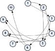
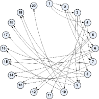
where the nonzero sub-block of TGsubscript𝑇𝐺T_{G} lies in rd1×rd1superscriptsubscript𝑟subscript𝑑1subscript𝑟subscript𝑑1\mathbb{R}^{r_{d_{1}}\times r_{d_{1}}}. We can also illustrate the communication graphs for the cases αΔ3𝛼subscriptΔ3\alpha\in\Delta_{3} and αΔ4𝛼subscriptΔ4\alpha\in\Delta_{4} with dp=2subscript𝑑𝑝2d_{p}=2 as seen in Fig. 3 and 3.

Refer to caption
Refer to caption
Figure 3: Graph representation of the network communication of the set-up algorithm. (a) Communication directed graph for the case αΔ3,dp=2formulae-sequence𝛼subscriptΔ3subscript𝑑𝑝2\alpha\in\Delta_{3},d_{p}=2. (b) Communication directed graph for the case αΔ4,dp=2formulae-sequence𝛼subscriptΔ4subscript𝑑𝑝2\alpha\in\Delta_{4},d_{p}=2.

For a given algorithm, the communication complexity is defined as the sum of the size of all communicated messages. For simplicity, let us consider the worst case scenario, where each processor is assigned more than one monomial and sends all of its assigned βh,γsubscript𝛽delimited-⟨⟩delimited-⟨⟩𝛾\beta_{\langle h\rangle,\langle\gamma\rangle} and Hh,γsubscript𝐻delimited-⟨⟩delimited-⟨⟩𝛾H_{\langle h\rangle,\langle\gamma\rangle} coefficients to other processors. In this case, the algorithm assigns 𝚏𝚕𝚘𝚘𝚛(LN)card(Wdp)𝚏𝚕𝚘𝚘𝚛𝐿𝑁cardsubscript𝑊subscript𝑑𝑝\mathtt{floor}(\frac{L}{N})\cdot\text{card}(W_{d_{p}}) of the βh,γsubscript𝛽delimited-⟨⟩delimited-⟨⟩𝛾\beta_{\langle h\rangle,\langle\gamma\rangle} coefficients, each of size 1, and (𝚏𝚕𝚘𝚘𝚛(LN)+𝚏𝚕𝚘𝚘𝚛(MN))card(Wdp)𝚏𝚕𝚘𝚘𝚛𝐿𝑁𝚏𝚕𝚘𝚘𝚛𝑀𝑁cardsubscript𝑊subscript𝑑𝑝\left(\mathtt{floor}(\frac{L}{N})+\mathtt{floor}(\frac{M}{N})\right)\cdot\text{card}(W_{d_{p}}) of the Hh,γsubscript𝐻delimited-⟨⟩delimited-⟨⟩𝛾H_{\langle h\rangle,\langle\gamma\rangle} coefficients, each of size n2superscript𝑛2n^{2}, to each processor. Thus the communication complexity of the algorithm per processor and per iteration is

card(Wdp)(𝚏𝚕𝚘𝚘𝚛(LN)+𝚏𝚕𝚘𝚘𝚛(MN)n2).cardsubscript𝑊subscript𝑑𝑝𝚏𝚕𝚘𝚘𝚛𝐿𝑁𝚏𝚕𝚘𝚘𝚛𝑀𝑁superscript𝑛2\text{card}(W_{d_{p}})\left(\mathtt{floor}\left(\frac{L}{N}\right)+\mathtt{floor}\left(\frac{M}{N}\right)n^{2}\right). (44)

This indicates that increasing the number of processors (up to M𝑀M) actually leads to less communication overhead per processor and improves the scalability of the algorithm. By substituting for card(Wdp)subscript𝑊subscript𝑑𝑝(W_{d_{p}}) from (25), L𝐿L from (26) and M𝑀M from (27) and considering large l𝑙l and n𝑛n, the communication complexity per processor at each Polya’s iteration is ldpa+d2n2similar-toabsentsuperscript𝑙subscript𝑑𝑝𝑎subscript𝑑2superscript𝑛2\sim l^{d_{pa}+d_{2}}n^{2} having N=L0𝑁subscript𝐿0N=L_{0} processors, ldpa+d2d1n2similar-toabsentsuperscript𝑙subscript𝑑𝑝𝑎subscript𝑑2subscript𝑑1superscript𝑛2\sim l^{d_{pa}+d_{2}-d_{1}}n^{2} having N=L𝑁𝐿N=L processors and ldpn2similar-toabsentsuperscript𝑙subscript𝑑𝑝superscript𝑛2\sim l^{d_{p}}n^{2} having N=M𝑁𝑀N=M processors.

IV PARALLEL SDP SOLVER

In this section, we describe the steps of our primal-dual interior-point algorithm and show how, for the LMIs in (15) and (16), these steps can be distributed in a distributed-computing, distributed-memory environment.

IV-A Interior-point methods

Interior-point methods define a popular class of algorithms for solving linear and semi-definite programming problems. The most widely accepted interior-point algorithms are dual scaling [44, 45], primal-dual [46, 47, 48] and cutting-plane/spectral bundle [49, 50, 51]. In this paper, we use the central-path-following primal-dual algorithm described in [48] and [27]. Although we found it possible to use dual-scaling algorithms, we chose to pursue a primal-dual algorithm because, in general, primal-dual algorithms converge faster [48, 45] while still preserving the structure of the solution (see (59)) at each iteration. We prefer primal-dual to cutting plane/spectral bundle methods because, as we show in Section IV-D, the centralized part of our primal-dual algorithm consists of solving a symmetric system of linear equations (see (80)), whereas for the cutting plane/spectral bundle algorithm, the centralized computation would consist of solving a constrained quadratic program (see [50][51]) with number of variables equal to the size of the system of linear equations. Because centralized computation is the limiting factor in a parallel algorithm, and because solving symmetric linear equations is simpler than solving a quadratic programming problem, we chose the primal-dual approach.

The choice of a central path-following primal-dual algorithm as in [48] and [52] was motivated by results in [53] which demonstrated better convergence, accuracy and robustness over the other types of primal-dual algorithms. More specifically, we chose the approach in [48] over [52] because unlike the Schur complement matrix (SCM) approach of the algorithm in [52], the SCM of [48] is symmetric and only the upper-triangular elements need to be sent/received by the processors. This leads to less communication overhead. The other reason for choosing [48] is that the symmetric SCM of the algorithm in [48] can be factorized using Cholesky factorization, whereas the non-symmetric SCM of [52] must be factorized by LU factorization (LU factorization is roughly twice as expensive as Cholesky factorization). Since factorization of SCM comprises the main portion of centralized computation in our algorithm, it is crucial for us to use computationally cheaper factorization methods to achieve better scalability.

In the primal-dual algorithm, both primal and dual problems are solved by iteratively calculating primal and dual step directions and step sizes, and applying these to the primal and dual variables. Let X𝑋X be the primal variable and y𝑦y and Z𝑍Z be the dual variables. At each iteration, the variables are updated as

Xk+1subscript𝑋𝑘1\displaystyle X_{k+1} =Xk+tpΔXabsentsubscript𝑋𝑘subscript𝑡𝑝Δ𝑋\displaystyle=X_{k}+t_{p}\Delta X (45)
yk+1subscript𝑦𝑘1\displaystyle y_{k+1} =yk+tdΔyabsentsubscript𝑦𝑘subscript𝑡𝑑Δ𝑦\displaystyle=y_{k}+t_{d}\Delta y (46)
Zk+1subscript𝑍𝑘1\displaystyle Z_{k+1} =Zk+tdΔZ,absentsubscript𝑍𝑘subscript𝑡𝑑Δ𝑍\displaystyle=Z_{k}+t_{d}\Delta Z, (47)

where ΔXΔ𝑋\Delta X, ΔyΔ𝑦\Delta y, and ΔZΔ𝑍\Delta Z are Newton’s search direction and tpsubscript𝑡𝑝t_{p} and tdsubscript𝑡𝑑t_{d} are primal and dual step sizes. We choose the step sizes using a standard line-search between 00 and 111 with the constraint that Xk+1subscript𝑋𝑘1X_{k+1} and Zk+1subscript𝑍𝑘1Z_{k+1} remain positive semi-definite. We use a Newton’s search direction given by

ΔX=ΔX^+ΔX¯Δ𝑋Δ^𝑋Δ¯𝑋\displaystyle\Delta X=\Delta\widehat{X}+\Delta\overline{X} (48)
Δy=Δy^+Δy¯Δ𝑦Δ^𝑦Δ¯𝑦\displaystyle\Delta y=\Delta\widehat{y}+\Delta\overline{y} (49)
ΔZ=ΔZ^+ΔZ¯,Δ𝑍Δ^𝑍Δ¯𝑍\displaystyle\Delta Z=\Delta\widehat{Z}+\Delta\overline{Z}, (50)

where ΔX^Δ^𝑋\Delta\widehat{X}, Δy^Δ^𝑦\Delta\widehat{y} and ΔZ^Δ^𝑍\Delta\widehat{Z} are the predictor step directions and ΔX¯Δ¯𝑋\Delta\overline{X}, Δy¯Δ¯𝑦\Delta\overline{y}, and ΔZ¯Δ¯𝑍\Delta\overline{Z} are the corrector step directions. As per [48], the predictor step directions are found as

Δy^=Ω1(a+B(Z1GX))Δ^𝑦superscriptΩ1𝑎𝐵superscript𝑍1𝐺𝑋\displaystyle\Delta\widehat{y}=\Omega^{-1}\left(-a+B(Z^{-1}GX)\right) (51)
ΔX^=X+Z1GBT(Δy^)XΔ^𝑋𝑋superscript𝑍1𝐺superscript𝐵𝑇Δ^𝑦𝑋\displaystyle\Delta\widehat{X}=-X+Z^{-1}GB^{T}(\Delta\widehat{y})X (52)
ΔZ^=BT(y)ZC+BT(Δy^),Δ^𝑍superscript𝐵𝑇𝑦𝑍𝐶superscript𝐵𝑇Δ^𝑦\displaystyle\Delta\widehat{Z}=B^{T}(y)-Z-C+B^{T}(\Delta\widehat{y}), (53)

where C𝐶C and the operators B𝐵B and BTsuperscript𝐵𝑇B^{T} are as defined in the previous section,

G=BT(y)+Z+C,𝐺superscript𝐵𝑇𝑦𝑍𝐶G=-B^{T}(y)+Z+C, (54)

and

Ω=[B(Z1BT(e1)X)B(Z1BT(ek)X)].Ωdelimited-[]𝐵superscript𝑍1superscript𝐵𝑇subscript𝑒1𝑋𝐵superscript𝑍1superscript𝐵𝑇subscript𝑒𝑘𝑋\Omega=\left[B(Z^{-1}B^{T}(e_{1})X)\;\cdots\;B(Z^{-1}B^{T}(e_{k})X)\right]. (55)

Recall that e1,,eksubscript𝑒1subscript𝑒𝑘e_{1},...,e_{k} are the standard basis for ksuperscript𝑘\mathbb{R}^{k}. Once we have the predictor step directions, we can calculate the corrector step directions as per [48]. Let μ=13tr(ZX)𝜇13𝑡𝑟𝑍𝑋\mu=\dfrac{1}{3}tr(ZX). The corrector step directions are

Δy¯=Ω1(B(μZ1)B(Z1ΔZ^ΔX^))Δ¯𝑦superscriptΩ1𝐵𝜇superscript𝑍1𝐵superscript𝑍1Δ^𝑍Δ^𝑋\displaystyle\Delta\overline{y}=\Omega^{-1}\left(B(\mu Z^{-1})-B(Z^{-1}\Delta\widehat{Z}\Delta\widehat{X})\right) (56)
ΔX¯=μZ1Z1ΔZ^ΔX^Z1ΔZ¯XΔ¯𝑋𝜇superscript𝑍1superscript𝑍1Δ^𝑍Δ^𝑋superscript𝑍1Δ¯𝑍𝑋\displaystyle\Delta\overline{X}=\mu Z^{-1}-Z^{-1}\Delta\widehat{Z}\Delta\widehat{X}-Z^{-1}\Delta\overline{Z}X (57)
ΔZ¯=BT(Δy¯).Δ¯𝑍superscript𝐵𝑇Δ¯𝑦\displaystyle\Delta\overline{Z}=B^{T}(\Delta\overline{y}). (58)

The stopping criterion is |aTytr(CX)|ϵsuperscript𝑎𝑇𝑦𝑡𝑟𝐶𝑋italic-ϵ|a^{T}y-tr(CX)|\leq\epsilon. Information regarding the selection of starting points and convergence of different variants of interior-point primal-dual algorithm, including the algorithm we use in this paper are presented in [46][47] and [48].

IV-B Structure of SDP Variables

The key algorithmic insight of this paper which allows us to use the primal-dual approach presented in [48] is that by choosing an initial value for the primal variable with a certain block structure corresponding to the distributed structure of the processors, the algorithm will preserve this structure at every iteration. Specifically, we define the following structured block-diagonal subspace where each block corresponds to a single processor.

Sl,m,nsubscript𝑆𝑙𝑚𝑛\displaystyle S_{l,m,n} :={Y(l+m)n×(l+m)n:\displaystyle:=\{Y\subset\mathbb{R}^{(l+m)n\times(l+m)n}:
Y=diag(Y1,Yl,Yl+1,Yl+m)forYin×n}\displaystyle Y=\text{diag}(Y_{1},\cdots Y_{l},Y_{l+1},\cdots Y_{l+m})\;\text{for}\;Y_{i}\in\mathbb{R}^{n\times n}\} (59)

According to the following theorem, the subspace Sl,m,nsubscript𝑆𝑙𝑚𝑛S_{l,m,n} is invariant under Newton’s iteration in the sense that when the algorithm in [48] is applied to the SDP problem defined by the polynomial optimization problem with initial value of the primal variable X0Sl,m,nsubscript𝑋0subscript𝑆𝑙𝑚𝑛X_{0}\in S_{l,m,n}, then the primal variable remains in the subspace at every Newton’s iteration Xksubscript𝑋𝑘X_{k}.

Theorem 3

Consider the SDP problem defined in (28) and (30) with elements given by (32), (34) and (38). Suppose L𝐿L and M𝑀M are the cardinalities of Wdp+d1subscript𝑊subscript𝑑𝑝subscript𝑑1W_{d_{p}+d_{1}} and Wdpa+d2subscript𝑊subscript𝑑𝑝𝑎subscript𝑑2W_{d_{pa}+d_{2}}. If (45), (46) and (47) are initialized by

X0SL,M,n,y0K,Z0SL,M,n,formulae-sequencesubscript𝑋0subscript𝑆𝐿𝑀𝑛formulae-sequencesubscript𝑦0superscript𝐾subscript𝑍0subscript𝑆𝐿𝑀𝑛X_{0}\in S_{L,M,n},\quad y_{0}\in\mathbb{R}^{K},\quad Z_{0}\in S_{L,M,n}, (60)

then for all k𝑘k\in\mathbb{N},

XkSL,M,n,ZkSL,M,n.formulae-sequencesubscript𝑋𝑘subscript𝑆𝐿𝑀𝑛subscript𝑍𝑘subscript𝑆𝐿𝑀𝑛X_{k}\in S_{L,M,n},\quad Z_{k}\in S_{L,M,n}. (61)
Proof:

We proceed by induction. First, suppose for some k,𝑘k\in\mathbb{N},

XkSL,M,nandZkSL,M,n.formulae-sequencesubscript𝑋𝑘subscript𝑆𝐿𝑀𝑛andsubscript𝑍𝑘subscript𝑆𝐿𝑀𝑛X_{k}\in S_{L,M,n}\quad\text{and}\quad Z_{k}\in S_{L,M,n}. (62)

We would like to show that this implies Xk+1,Zk+1SL,M,nsubscript𝑋𝑘1subscript𝑍𝑘1subscript𝑆𝐿𝑀𝑛X_{k+1},Z_{k+1}\in S_{L,M,n}. To see this, observe that according to (45)

Xk+1=Xk+tpΔXkfor allk.formulae-sequencesubscript𝑋𝑘1subscript𝑋𝑘subscript𝑡𝑝Δsubscript𝑋𝑘for all𝑘X_{k+1}=X_{k}+t_{p}\Delta X_{k}\quad\text{for all}\;\,k\in\mathbb{N}. (63)

From (48), ΔXkΔsubscript𝑋𝑘\Delta X_{k} can be written as

ΔXk=ΔX^k+ΔX¯kfor allk.formulae-sequenceΔsubscript𝑋𝑘Δsubscript^𝑋𝑘Δsubscript¯𝑋𝑘for all𝑘\Delta X_{k}=\Delta\widehat{X}_{k}+\Delta\overline{X}_{k}\quad\text{for all}\;\,k\in\mathbb{N}. (64)

To find the structure of ΔXkΔsubscript𝑋𝑘\Delta X_{k}, we focus on the structures of ΔX^kΔsubscript^𝑋𝑘\Delta\widehat{X}_{k} and ΔX¯kΔsubscript¯𝑋𝑘\Delta\overline{X}_{k} individually. Using (52), ΔX^kΔsubscript^𝑋𝑘\Delta\widehat{X}_{k} is

ΔX^k=Xk+Zk1GkBT(Δy^k)Xkfor allk.formulae-sequenceΔsubscript^𝑋𝑘subscript𝑋𝑘superscriptsubscript𝑍𝑘1subscript𝐺𝑘superscript𝐵𝑇Δsubscript^𝑦𝑘subscript𝑋𝑘for all𝑘\Delta\widehat{X}_{k}=-X_{k}+Z_{k}^{-1}G_{k}B^{T}(\Delta\widehat{y}_{k})X_{k}\quad\text{for all}\;\,k\in\mathbb{N}. (65)

where according to (54), Gksubscript𝐺𝑘G_{k} is

Gk=CBT(yk)+Zkfor allk.formulae-sequencesubscript𝐺𝑘𝐶superscript𝐵𝑇subscript𝑦𝑘subscript𝑍𝑘for all𝑘G_{k}=C-B^{T}(y_{k})+Z_{k}\quad\text{for all}\;\,k\in\mathbb{N}. (66)

First we examine the structure of Gksubscript𝐺𝑘G_{k}. According to the definition of C𝐶C and Bisubscript𝐵𝑖B_{i} in (32) and (34), and the definition of BT(y)superscript𝐵𝑇𝑦B^{T}(y) in (31), we know that

CSL,M,n,BT:KSL,M,n.:𝐶subscript𝑆𝐿𝑀𝑛superscript𝐵𝑇maps-tosuperscript𝐾subscript𝑆𝐿𝑀𝑛C\in S_{L,M,n},\quad B^{T}:\mathbb{R}^{K}\mapsto S_{L,M,n}. (67)

Since all the terms on the right hand side of (66) are in SL,M,nsubscript𝑆𝐿𝑀𝑛S_{L,M,n} and SL,M,nsubscript𝑆𝐿𝑀𝑛S_{L,M,n} is a subspace, we conclude

GkSL,M,n.subscript𝐺𝑘subscript𝑆𝐿𝑀𝑛G_{k}\in S_{L,M,n}.\vspace*{-0.05in} (68)

Returning to (65), using our assumption in (62) and noting that the structure of the matrices in SL,M,nsubscript𝑆𝐿𝑀𝑛S_{L,M,n} is also preserved through multiplication and inversion, we conclude

ΔX^kSL,M,n.Δsubscript^𝑋𝑘subscript𝑆𝐿𝑀𝑛\Delta\widehat{X}_{k}\in S_{L,M,n}. (69)

Using (57), the second term in (64) is

ΔX¯k=μZk1Zk1ΔZ^kΔX^kZk1ΔZ¯kXkfor allk.formulae-sequenceΔsubscript¯𝑋𝑘𝜇superscriptsubscript𝑍𝑘1superscriptsubscript𝑍𝑘1Δsubscript^𝑍𝑘Δsubscript^𝑋𝑘superscriptsubscript𝑍𝑘1Δsubscript¯𝑍𝑘subscript𝑋𝑘for all𝑘\Delta\overline{X}_{k}=\mu Z_{k}^{-1}-Z_{k}^{-1}\Delta\widehat{Z}_{k}\Delta\widehat{X}_{k}-Z_{k}^{-1}\Delta\overline{Z}_{k}X_{k}\quad\text{for all}\;\,k\in\mathbb{N}. (70)

To determine the structure of ΔX¯kΔsubscript¯𝑋𝑘\Delta\overline{X}_{k}, first we investigate the structure of ΔZ^kΔsubscript^𝑍𝑘\Delta\widehat{Z}_{k} and ΔZ¯kΔsubscript¯𝑍𝑘\Delta\overline{Z}_{k}. According to (53) and (58) we have

ΔZ^k=BT(yk)ZkC+BT(Δy^k)Δsubscript^𝑍𝑘superscript𝐵𝑇subscript𝑦𝑘subscript𝑍𝑘𝐶superscript𝐵𝑇Δsubscript^𝑦𝑘\displaystyle\Delta\widehat{Z}_{k}=B^{T}(y_{k})-Z_{k}-C+B^{T}(\Delta\widehat{y}_{k}) for allkfor all𝑘\displaystyle\text{for all}\;\,k\in\mathbb{N} (71)
ΔZ¯k=BT(Δy¯k)Δsubscript¯𝑍𝑘superscript𝐵𝑇Δsubscript¯𝑦𝑘\displaystyle\Delta\overline{Z}_{k}=B^{T}(\Delta\overline{y}_{k}) for allk.for all𝑘\displaystyle\text{for all}\;\,k\in\mathbb{N}. (72)

Since all the terms in the right hand side of (71) and (72) are in SL,M,nsubscript𝑆𝐿𝑀𝑛S_{L,M,n}, then

ΔZ^kSL,M,n,ΔZ¯kSL,M,n.formulae-sequenceΔsubscript^𝑍𝑘subscript𝑆𝐿𝑀𝑛Δsubscript¯𝑍𝑘subscript𝑆𝐿𝑀𝑛\Delta\widehat{Z}_{k}\in S_{L,M,n},\quad\Delta\overline{Z}_{k}\in S_{L,M,n}. (73)

Recalling (69), (70) and our assumption in (62), we have

ΔX¯kSL,M,n.Δsubscript¯𝑋𝑘subscript𝑆𝐿𝑀𝑛\Delta\overline{X}_{k}\in S_{L,M,n}. (74)

According to (69), (73) and (74), the total step directions are in SL,M,nsubscript𝑆𝐿𝑀𝑛S_{L,M,n},

ΔXk=ΔX^k+ΔX¯kSL,M,nΔsubscript𝑋𝑘Δsubscript^𝑋𝑘Δsubscript¯𝑋𝑘subscript𝑆𝐿𝑀𝑛\displaystyle\Delta X_{k}=\Delta\widehat{X}_{k}+\Delta\overline{X}_{k}\in S_{L,M,n} (75)
ΔZk=ΔZ^k+ΔZ¯kSL,M,n,Δsubscript𝑍𝑘Δsubscript^𝑍𝑘Δsubscript¯𝑍𝑘subscript𝑆𝐿𝑀𝑛\displaystyle\Delta Z_{k}=\Delta\widehat{Z}_{k}+\Delta\overline{Z}_{k}\in S_{L,M,n}, (76)

and it follows that

Xk+1=Xk+tpΔXkSL,M,nsubscript𝑋𝑘1subscript𝑋𝑘subscript𝑡𝑝Δsubscript𝑋𝑘subscript𝑆𝐿𝑀𝑛\displaystyle X_{k+1}=X_{k}+t_{p}\Delta X_{k}\in S_{L,M,n} (77)
Zk+1=Zk+tpΔZkSL,M,n.subscript𝑍𝑘1subscript𝑍𝑘subscript𝑡𝑝Δsubscript𝑍𝑘subscript𝑆𝐿𝑀𝑛\displaystyle Z_{k+1}=Z_{k}+t_{p}\Delta Z_{k}\in S_{L,M,n}. (78)

Thus, for any yK𝑦superscript𝐾y\in\mathbb{R}^{K} and k𝑘k\in\mathbb{N}, if Xk,ZkSL,M,nsubscript𝑋𝑘subscript𝑍𝑘subscript𝑆𝐿𝑀𝑛X_{k},Z_{k}\in S_{L,M,n}, we have Xk+1,Zk+1SL,M,nsubscript𝑋𝑘1subscript𝑍𝑘1subscript𝑆𝐿𝑀𝑛X_{k+1},Z_{k+1}\in S_{L,M,n}. Since we have assumed that the initial values X0,Z0SL,M,nsubscript𝑋0subscript𝑍0subscript𝑆𝐿𝑀𝑛X_{0},Z_{0}\in S_{L,M,n}, we conclude by induction that XkSL,M,nsubscript𝑋𝑘subscript𝑆𝐿𝑀𝑛X_{k}\in S_{L,M,n} and ZkSL,M,nsubscript𝑍𝑘subscript𝑆𝐿𝑀𝑛Z_{k}\in S_{L,M,n} for all k𝑘k\in\mathbb{N}. ∎

IV-C Parallel Implementation

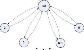
In this section, a parallel algorithm for solving the SDP problems associated with Polya’s algorithm is provided. We show how to map the block-diagonal structure of the primal variable and Newton updates described in Section IV-A to a parallel computing structure consisting of a central root processor with N𝑁N slave processors. Note that processor steps are simultaneous and transitions between root and processor steps are synchronous. Processors are idle when root is active and vice-versa. A C++ implementation of this algorithm, using MPI and Blas/Lapack libraries is provided at: www.sites.google.com/a/asu.edu/kamyar/software. Let N𝑁N be the number of available processors and J=𝚏𝚕𝚘𝚘𝚛(L+MN)𝐽𝚏𝚕𝚘𝚘𝚛𝐿𝑀𝑁J=\mathtt{floor}\left(\frac{L+M}{N}\right). As per Algorithm 1, we assume processor i𝑖i has access to the sub-blocks 𝐂¯isubscript¯𝐂𝑖\mathbf{\overline{C}}_{i} and B¯j,isubscript¯B𝑗𝑖\mathbf{\overline{\textbf{B}}}_{j,i} defined in (39) and (40) for j=1,,K𝑗1𝐾j=1,\cdots,K. Be aware that minor parts of Algorithm 2 have been abridged in order to simplify the presentation.

IV-D Computational Complexity Analysis: SDP Algorithm

NC \subset P is defined to be the class of problems which can be solved in a poly-logarithmic number of steps using a polynomially number processors and is often considered to be the class of problems that can be parallelized efficiently. The class P-complete is a set of problems which are equivalent up to an NC reduction, but contains no problem in NC and is thought to be the simplest class of ”inherently sequential” problems. It has been proven that Linear Programming (LP) is P-complete [54] and SDP is P-hard (at least as hard as any P-complete problem) and thus is unlikely to admit a general-purpose parallel solution. Given this fact and given the observation that the problem we are trying to solve is NP-hard, it is important to thoroughly understand the complexity of the algorithms we are proposing and how this complexity scales with various parameters which define the size of the problem. To better understand these issues, we have broken our complexity analysis down into several cases which should be of interest to the control community. Note that the cases below do not discuss memory complexity. This is because in the cases when a sufficient number of processors are available, for a system with n𝑛n states, the memory requirements per block are simply proportional to n2superscript𝑛2n^{2}.

1) Case 1: Systems with large number of states

Suppose we are considering a problem with n𝑛n states. For

Inputs: C¯i,B¯j,isubscript¯C𝑖subscript¯B𝑗𝑖\overline{\textbf{C}}_{i},\overline{\textbf{B}}_{j,i} for i=1,,N𝑖1𝑁i=1,\cdots,N and j=1,,K𝑗1𝐾j=1,\cdots,K - the sub-blocks of the SDP elements provided to processor i𝑖i by the set-up algorithm.
Processors Initialization step:
for i=1,,N𝑖1𝑁i=1,\cdots,N, processor i𝑖i do
       Initialize primal and dual variables 𝐗i0subscriptsuperscript𝐗0𝑖\mathbf{X}^{0}_{i}, 𝐙i0subscriptsuperscript𝐙0𝑖\mathbf{Z}^{0}_{i} and y0superscript𝑦0y^{0} as
𝐗i0={I(J+1)n,0i<L+MNJIJn,L+MNJi<N,,subscriptsuperscript𝐗0𝑖casessubscript𝐼𝐽1𝑛0𝑖𝐿𝑀𝑁𝐽subscript𝐼𝐽𝑛𝐿𝑀𝑁𝐽𝑖𝑁\mathbf{X}^{0}_{i}=\begin{cases}I_{(J+1)n},&0\leq i<L+M-NJ\\ I_{Jn},&L+M-NJ\leq i<N,\end{cases},
𝐙i0=𝐗i0andy0=0K,formulae-sequencesubscriptsuperscript𝐙0𝑖subscriptsuperscript𝐗0𝑖andsuperscript𝑦00superscript𝐾\mathbf{Z}^{0}_{i}=\mathbf{X}^{0}_{i}\quad\text{and}\quad y^{0}=\vec{0}\in\mathbb{R}^{K},
Calculate the complementary slackness [49] Si=tr(𝐙i0𝐗i0)subscript𝑆𝑖𝑡𝑟superscriptsubscript𝐙𝑖0superscriptsubscript𝐗𝑖0S_{i}=tr(\mathbf{Z}_{i}^{0}\mathbf{X}_{i}^{0}). Send Sisubscript𝑆𝑖S_{i} to processor root.
Root Initialization step:
Root processor do
  Calculate the barrier parameter [49] μ=13i=1NSi𝜇13superscriptsubscript𝑖1𝑁subscript𝑆𝑖\mu=\frac{1}{3}\sum_{i=1}^{N}S_{i}.   Set the SDP element a=1K𝑎1superscript𝐾a=\vec{1}\in\mathbb{R}^{K}.
Processors step 1:
for i=1,,N𝑖1𝑁i=1,\cdots,N, processor i𝑖i do
       for k=1,,K𝑘1𝐾k=1,\cdots,K do
             Calculate the elements of Ω1subscriptΩ1\Omega_{1} (R-H-S of (80))
ωi,k=tr(B¯k,i(𝐙i)1(j=1KyjB¯j,i+𝐙i+𝐂¯i)𝐗i)subscript𝜔𝑖𝑘𝑡𝑟subscript¯B𝑘𝑖superscriptsubscript𝐙𝑖1superscriptsubscript𝑗1𝐾subscript𝑦𝑗subscript¯B𝑗𝑖subscript𝐙𝑖subscript¯𝐂𝑖subscript𝐗𝑖\omega_{i,k}=tr\left(\mathbf{\overline{\textbf{B}}}_{k,i}(\mathbf{{Z}}_{i})^{-1}\left(-\sum_{j=1}^{K}y_{j}\mathbf{\overline{\textbf{B}}}_{j,i}+\mathbf{Z}_{i}+\mathbf{\overline{C}}_{i}\right)\mathbf{X}_{i}\right)
for l=1,,K𝑙1𝐾l=1,\cdots,K do
                   Calculate the elements of the SCM as
λi,k,l=tr(B¯k,i(𝐙i)1B¯l,i𝐗i)subscript𝜆𝑖𝑘𝑙𝑡𝑟subscript¯B𝑘𝑖superscriptsubscript𝐙𝑖1subscript¯B𝑙𝑖subscript𝐗𝑖\lambda_{i,k,l}=tr\left(\mathbf{\overline{\textbf{B}}}_{k,i}(\mathbf{{Z}}_{i})^{-1}\mathbf{\overline{\textbf{B}}}_{l,i}\mathbf{X}_{i}\right) (79)
            
      Send ωi,ksubscript𝜔𝑖𝑘\omega_{i,k} and λi,k,lsubscript𝜆𝑖𝑘𝑙\lambda_{i,k,l}, k=1,,K𝑘1𝐾k=1,\cdots,K and l=1,,K𝑙1𝐾l=1,\cdots,K to root processor.
Root step 1:
Root processor do
  Construct the R-H-S of (80) and the SCM as
Ω1=(i=1Nωi,1i=1Nωi,2i=1Nωi,K)aandsubscriptΩ1superscriptsubscript𝑖1𝑁subscript𝜔𝑖1missing-subexpressionmissing-subexpressionsuperscriptsubscript𝑖1𝑁subscript𝜔𝑖2missing-subexpressionmissing-subexpressionmissing-subexpressionmissing-subexpressionsuperscriptsubscript𝑖1𝑁subscript𝜔𝑖𝐾missing-subexpressionmissing-subexpression𝑎and\hskip 7.22743pt\Omega_{1}=\left(\begin{array}[]{ccc}\sum_{i=1}^{N}\omega_{i,1}\\ \sum_{i=1}^{N}\omega_{i,2}\\ \vdots\\ \sum_{i=1}^{N}\omega_{i,K}\end{array}\right)-a\quad\text{and}
Λ=[(i=1Nλi,1,1i=1Nλi,2,1i=1Nλi,K,1),,(i=1Nλi,1,Ki=1Nλi,2,Ki=1Nλi,K,K)]Λsuperscriptsubscript𝑖1𝑁subscript𝜆𝑖11missing-subexpressionmissing-subexpressionsuperscriptsubscript𝑖1𝑁subscript𝜆𝑖21missing-subexpressionmissing-subexpressionmissing-subexpressionmissing-subexpressionsuperscriptsubscript𝑖1𝑁subscript𝜆𝑖𝐾1missing-subexpressionmissing-subexpressionsuperscriptsubscript𝑖1𝑁subscript𝜆𝑖1𝐾missing-subexpressionmissing-subexpressionsuperscriptsubscript𝑖1𝑁subscript𝜆𝑖2𝐾missing-subexpressionmissing-subexpressionmissing-subexpressionmissing-subexpressionsuperscriptsubscript𝑖1𝑁subscript𝜆𝑖𝐾𝐾missing-subexpressionmissing-subexpression\Lambda=\left[\left(\begin{array}[]{ccc}\sum_{i=1}^{N}\lambda_{i,1,1}\\ \sum_{i=1}^{N}\lambda_{i,2,1}\\ \vdots\\ \sum_{i=1}^{N}\lambda_{i,K,1}\end{array}\right),\cdots,\left(\begin{array}[]{ccc}\sum_{i=1}^{N}\lambda_{i,1,K}\\ \sum_{i=1}^{N}\lambda_{i,2,K}\\ \vdots\\ \sum_{i=1}^{N}\lambda_{i,K,K}\end{array}\right)\right]
    Solve the following system of equations for the predictor dual step Δy^KΔ^𝑦superscript𝐾{\Delta\widehat{y}}\in\mathbb{R}^{K} and send     Δy^Δ^𝑦{\Delta\widehat{y}} to all processors.
ΛΔy^=Ω1ΛΔ^𝑦subscriptΩ1\hskip 3.61371pt\Lambda{\Delta\widehat{y}}=\Omega_{1} (80)
Algorithm 2 The parallel SDP solver algorithm
Processors step 2:
for i=1,,N𝑖1𝑁i=1,\cdots,N, processor i𝑖i do
       Calculate the predictor step directions
Δ𝐗^iΔsubscript^𝐗𝑖\displaystyle\Delta\mathbf{\widehat{X}}_{i} =𝐗iabsentsubscript𝐗𝑖\displaystyle=-\mathbf{X}_{i}
+(\displaystyle+( 𝐙i)1(j=1KyjB¯j,i+𝐙i+𝐂¯i)j=1KΔy^jB¯j,i𝐗i,\displaystyle\mathbf{{Z}}_{i})^{-1}\left(-\sum_{j=1}^{K}y_{j}\mathbf{\overline{\textbf{B}}}_{j,i}+\mathbf{Z}_{i}+\mathbf{\overline{C}}_{i}\right)\sum_{j=1}^{K}\Delta\widehat{y}_{j}\,\mathbf{\overline{\textbf{B}}}_{j,i}\;\mathbf{X}_{i},
Δ𝐙^i=j=1KyjB¯j,i𝐙i𝐂¯i+j=1KΔy^jB¯j,i.Δsubscript^𝐙𝑖superscriptsubscript𝑗1𝐾subscript𝑦𝑗subscript¯B𝑗𝑖subscript𝐙𝑖subscript¯𝐂𝑖superscriptsubscript𝑗1𝐾Δsubscript^𝑦𝑗subscript¯B𝑗𝑖\Delta\mathbf{\widehat{Z}}_{i}=\sum_{j=1}^{K}y_{j}\mathbf{\overline{\textbf{B}}}_{j,i}-\mathbf{Z}_{i}-\mathbf{\overline{C}}_{i}+\sum_{j=1}^{K}\Delta\widehat{y}_{j}\mathbf{\overline{\textbf{B}}}_{j,i}.
for k=1,,K𝑘1𝐾k=1,\cdots,K do
             Calculate the elements of Ω2subscriptΩ2\Omega_{2} (R-H-S of (81))
δi,k=tr(B¯k,i(𝐙i)1),τi,k=tr(B¯k,i(𝐙i)1Δ𝐙^iΔ𝐗^i)formulae-sequencesubscript𝛿𝑖𝑘𝑡𝑟subscript¯B𝑘𝑖superscriptsubscript𝐙𝑖1subscript𝜏𝑖𝑘𝑡𝑟subscript¯B𝑘𝑖superscriptsubscript𝐙𝑖1Δsubscript^𝐙𝑖Δsubscript^𝐗𝑖\delta_{i,k}=tr(\mathbf{\overline{\textbf{B}}}_{k,i}(\mathbf{{Z}}_{i})^{-1}),\tau_{i,k}=tr(\mathbf{\overline{\textbf{B}}}_{k,i}(\mathbf{{Z}}_{i})^{-1}\Delta\mathbf{\widehat{Z}}_{i}\Delta\mathbf{\widehat{X}}_{i})
      Send δi,ksubscript𝛿𝑖𝑘\delta_{i,k} and τi,ksubscript𝜏𝑖𝑘\tau_{i,k}, k=1,,K𝑘1𝐾k=1,\cdots,K to root processor.
Root step 2:
Root processor do
  Construct the R-H-S of (81) as
Ω2=μsubscriptΩ2𝜇\displaystyle\Omega_{2}=\mu [i=1Nδi,1i=1Nδi,2i=1Nδi,K]Tlimit-fromsuperscriptmatrixsuperscriptsubscript𝑖1𝑁subscript𝛿𝑖1superscriptsubscript𝑖1𝑁subscript𝛿𝑖2superscriptsubscript𝑖1𝑁subscript𝛿𝑖𝐾𝑇\displaystyle\begin{bmatrix}\sum_{i=1}^{N}\delta_{i,1}&\sum_{i=1}^{N}\delta_{i,2}&\cdots&\sum_{i=1}^{N}\delta_{i,K}\end{bmatrix}^{T}-
[i=1Nτi,1i=1Nτi,2i=1Nτi,K]Tsuperscriptmatrixsuperscriptsubscript𝑖1𝑁subscript𝜏𝑖1superscriptsubscript𝑖1𝑁subscript𝜏𝑖2superscriptsubscript𝑖1𝑁subscript𝜏𝑖𝐾𝑇\displaystyle\begin{bmatrix}\sum_{i=1}^{N}\tau_{i,1}&\sum_{i=1}^{N}\tau_{i,2}&\cdots&\sum_{i=1}^{N}\tau_{i,K}\end{bmatrix}^{T}
  Solve the following system of equations for the corrector dual variable Δy¯Δ¯𝑦\Delta\overline{y} and send Δy¯Δ¯𝑦\Delta\overline{y}    to all processors.
ΛΔy¯=Ω2ΛΔ¯𝑦subscriptΩ2\Lambda\Delta\overline{y}=\Omega_{2} (81)
Processors step 3:
for i=1,,N𝑖1𝑁i=1,\cdots,N, processor i𝑖i do
       Calculate the corrector step directions as follows.
Δ𝐙¯i=j=1KΔy¯jB¯j,iΔsubscript¯𝐙𝑖superscriptsubscript𝑗1𝐾Δsubscript¯𝑦𝑗subscript¯B𝑗𝑖\Delta\mathbf{\overline{Z}}_{i}=\sum_{j=1}^{K}\Delta\overline{y}_{j}\mathbf{\overline{\textbf{B}}}_{j,i}\vspace*{-0.05in}
Δ𝐗¯i=(𝐙i)1(Δ𝐙¯i𝐗i+Δ𝐙^iΔ𝐗^i)+μ(𝐙i)1Δsubscript¯𝐗𝑖superscriptsubscript𝐙𝑖1Δsubscript¯𝐙𝑖subscript𝐗𝑖Δsubscript^𝐙𝑖Δsubscript^𝐗𝑖𝜇superscriptsubscript𝐙𝑖1\Delta\mathbf{\overline{X}}_{i}=-(\mathbf{{Z}}_{i})^{-1}(\Delta\mathbf{\overline{Z}}_{i}\mathbf{X}_{i}+\Delta\mathbf{\widehat{Z}}_{i}\Delta\mathbf{\widehat{X}}_{i})+\mu(\mathbf{{Z}}_{i})^{-1}\vspace*{-0.05in}
      Calculate primal dual step total step directions as follows.
Δ𝐗i=Δ𝐗^i+Δ𝐗¯i,Δ𝐙i=Δ𝐙^i+Δ𝐙¯i,Δy=Δy^+Δy¯.formulae-sequenceΔsubscript𝐗𝑖Δsubscript^𝐗𝑖Δsubscript¯𝐗𝑖formulae-sequenceΔsubscript𝐙𝑖Δsubscript^𝐙𝑖Δsubscript¯𝐙𝑖Δ𝑦Δ^𝑦Δ¯𝑦\Delta\mathbf{X}_{i}=\Delta\mathbf{\widehat{X}}_{i}+\Delta\mathbf{\overline{X}}_{i},\Delta\mathbf{Z}_{i}=\Delta\mathbf{\widehat{Z}}_{i}+\Delta\mathbf{\overline{Z}}_{i},\Delta{y}=\Delta\widehat{y}+\Delta\overline{y}.\vspace*{-0.05in}
Set primal step size tpsubscript𝑡𝑝t_{p} and dual step size tdsubscript𝑡𝑑t_{d} using an appropriate line search methos.
       Update primal and dual variables as
𝐗i𝐗i+tpΔ𝐗i,𝐙i𝐙i+tdΔ𝐙i,yy+tdΔyformulae-sequencesubscript𝐗𝑖subscript𝐗𝑖subscript𝑡𝑝Δsubscript𝐗𝑖formulae-sequencesubscript𝐙𝑖subscript𝐙𝑖subscript𝑡𝑑Δsubscript𝐙𝑖𝑦𝑦subscript𝑡𝑑Δ𝑦\mathbf{X}_{i}\equiv\mathbf{X}_{i}+t_{p}\Delta\mathbf{X}_{i},\quad\mathbf{Z}_{i}\equiv\mathbf{Z}_{i}+t_{d}\Delta\mathbf{Z}_{i},\quad y\equiv y+t_{d}\Delta{y}\vspace*{-0.15in}
Processors step 4:
for i=1,,N𝑖1𝑁i=1,\cdots,N, processor i𝑖i do
       Calculate the contribution to primal cost ϕ~i=tr(𝐂¯i𝐗i)subscript~italic-ϕ𝑖𝑡𝑟subscript¯𝐂𝑖subscript𝐗𝑖\tilde{\phi}_{i}=tr\left(\mathbf{\overline{C}}_{i}\mathbf{X}_{i}\right) and the complementary slack Si=tr(𝐙i𝐗i)subscript𝑆𝑖𝑡𝑟subscript𝐙𝑖subscript𝐗𝑖S_{i}=tr\left(\mathbf{Z}_{i}\mathbf{X}_{i}\right). Send Sisubscript𝑆𝑖S_{i} and ϕ~isubscript~italic-ϕ𝑖\tilde{\phi}_{i} to root processor.
Root step 4:
Root processor do
  Update the barrier parameter μ=13i=1NSi𝜇13superscriptsubscript𝑖1𝑁subscript𝑆𝑖\mu=\frac{1}{3}\sum_{i=1}^{N}S_{i}. Calculate primal and dual costs as   ϕ=i=1Nϕ~iandψ=aTyitalic-ϕsuperscriptsubscript𝑖1𝑁subscript~italic-ϕ𝑖and𝜓superscript𝑎𝑇𝑦\phi=\sum_{i=1}^{N}\tilde{\phi}_{i}\;\text{and}\;\psi=a^{T}y. If |ϕψ|>εitalic-ϕ𝜓𝜀|\phi-\psi|>\varepsilon, then go to Processors step 1; Otherwise   calculate the coefficients of P(α)𝑃𝛼P(\alpha) as Pi=j=1N~Ejy(j+N~i1))P_{i}=\sum_{j=1}^{\tilde{N}}E_{j}y_{(j+\tilde{N}i-1))} for i=1,,L0𝑖1subscript𝐿0i=1,\cdots,L_{0}.

this case, the most expensive part of the algorithm is the calculation of the Schur complement matrix ΛΛ\Lambda by the processors in Processors step 1 (and summed by the root in Root step 1, although we neglect this part). In particular, the computational complexity of the algorithm is determined by the number of operations required to calculate (79), restated here.

λi,k,l=tr(B¯k,i(𝐙i)1B¯l,i𝐗i)subscript𝜆𝑖𝑘𝑙𝑡𝑟subscript¯B𝑘𝑖superscriptsubscript𝐙𝑖1subscript¯B𝑙𝑖subscript𝐗𝑖\lambda_{i,k,l}=tr\left(\mathbf{\overline{\textbf{B}}}_{k,i}(\mathbf{{Z}}_{i})^{-1}\mathbf{\overline{\textbf{B}}}_{l,i}\mathbf{X}_{i}\right)\vspace*{-0.05in} (82)
fork=1,,Kandl=1,,K.formulae-sequencefor𝑘1𝐾and𝑙1𝐾\text{for}\quad k=1,\cdots,K\;\text{and}\quad l=1,\cdots,K.\vspace*{-0.05in}

Since the cost of n×n𝑛𝑛n\times n matrix-matrix multiplication is n3similar-toabsentsuperscript𝑛3\sim n^{3} and each of 𝐗i,𝐙i,B¯l,isubscript𝐗𝑖subscript𝐙𝑖subscript¯B𝑙𝑖\mathbf{X}_{i},\mathbf{{Z}}_{i},\mathbf{\overline{\textbf{B}}}_{l,i} has 𝚏𝚕𝚘𝚘𝚛(L+MN)𝚏𝚕𝚘𝚘𝚛𝐿𝑀𝑁\mathtt{floor}(\frac{L+M}{N}) number of blocks in n×nsuperscript𝑛𝑛\mathbb{R}^{n\times n}, the number of operations performed by the ithsuperscript𝑖𝑡i^{th} processor to calculate λi,k,lsubscript𝜆𝑖𝑘𝑙\lambda_{i,k,l} for k=1,,K𝑘1𝐾k=1,\cdots,K and l=1,,K𝑙1𝐾l=1,\cdots,K is

{𝚏𝚕𝚘𝚘𝚛(L+MN)K2n3N<L+MK2n3NL+Mcasessimilar-toabsent𝚏𝚕𝚘𝚘𝚛𝐿𝑀𝑁superscript𝐾2superscript𝑛3𝑁𝐿𝑀similar-toabsentsuperscript𝐾2superscript𝑛3𝑁𝐿𝑀\begin{cases}\sim\mathtt{floor}\left(\dfrac{L+M}{N}\right)K^{2}n^{3}\;&N<L+M\\ \sim K^{2}n^{3}\;&N\geq L+M\end{cases} (83)

at each iteration, where i=1,,N𝑖1𝑁i=1,\cdots,N. By substituting K𝐾K in (83) from (35), for NL+M𝑁𝐿𝑀N\geq L+M, each processor performs

((dp+l1)!)2(dp!)2((l1)!)2n7similar-toabsentsuperscriptsubscript𝑑𝑝𝑙12superscriptsubscript𝑑𝑝2superscript𝑙12superscript𝑛7\sim\dfrac{((d_{p}+l-1)!)^{2}}{(d_{p}!)^{2}((l-1)!)^{2}}n^{7} (84)

operations per iteration. Therefore, for systems with large n𝑛n and fixed dpsubscript𝑑𝑝d_{p} and l𝑙l, the number of operations per processor required to solve the SDP associated with parameter-dependent feasibility problem A(α)TP(α)+P(α)A(α)0,precedes𝐴superscript𝛼𝑇𝑃𝛼𝑃𝛼𝐴𝛼0A(\alpha)^{T}P(\alpha)+P(\alpha)A(\alpha)\prec 0, is proportional to n7superscript𝑛7n^{7}. Solving the LMI associated with the parameter-independent problem ATP+PA0precedessuperscriptA𝑇𝑃𝑃A0\mathrm{A}^{T}P+P\mathrm{A}\prec 0 using our algorithm or most of the SDP solvers such as [55, 27, 28] also requires O(n7)𝑂superscript𝑛7O(n^{7}) operations per processor. Therefore, if we have a sufficient number of processors, the proposed algorithm solves both the stability and robust stability problems by performing O(n7)𝑂superscript𝑛7O(n^{7}) operations per processor in this case.

2) Case 2: High Accuracy/Low Conservativity

In this case we consider the effect of raising Polya’s exponent. Consider the definition of simplex as follows.

Δ~l={αl,i=1lαi=r,αi0}subscript~Δ𝑙formulae-sequence𝛼superscript𝑙formulae-sequencesuperscriptsubscript𝑖1𝑙subscript𝛼𝑖𝑟subscript𝛼𝑖0\tilde{\Delta}_{l}=\left\{\alpha\in\mathbb{R}^{l},\sum_{i=1}^{l}\alpha_{i}=r,\alpha_{i}\geqslant 0\right\}\vspace*{-0.05in} (85)

Suppose we now define the accuracy of the algorithm as the largest value of r𝑟r found by the algorithm (if it exists) such that if the uncertain parameters lie inside the corresponding simplex, the stability of the system is verified. Typically, increasing Polya’s exponent d𝑑d in (10) improves the accuracy of the algorithm. If we again only consider Processor step 1, according to (84), the number of processor operations is independent of the Polya’s exponent d1subscript𝑑1d_{1} and d2subscript𝑑2d_{2}! Because this part of the algorithm does not vary with Polya’s exponent, we look at the root processing requirements associated with solving the systems of equations in (80) and (81) in Root step 1 using Cholesky factorization. Each of these systems consists of K𝐾K equations. The computational complexity of Cholesky factorization is O(K3)𝑂superscript𝐾3O(K^{3}). Thus the number of operations performed by the root processor is proportional to

K3=((dp+l1)!)3(dp!)3((l1)!)3n6.superscript𝐾3superscriptsubscript𝑑𝑝𝑙13superscriptsubscript𝑑𝑝3superscript𝑙13superscript𝑛6K^{3}=\dfrac{((d_{p}+l-1)!)^{3}}{(d_{p}!)^{3}((l-1)!)^{3}}n^{6}.\vspace*{-0.05in} (86)

In terms of communication complexity, the most significant operation between the root and other processors is sending and receiving λi,k,lsubscript𝜆𝑖𝑘𝑙\lambda_{i,k,l} for i=1,,N𝑖1𝑁i=1,\cdots,N, k=1,,K𝑘1𝐾k=1,\cdots,K and l=1,,K𝑙1𝐾l=1,\cdots,K in Processors step 1 and Root step 1. Thus the total communication cost for N𝑁N processors per iteration is

NK2=N((dp+l1)!)2(dp!)2((l1)!)2n4.similar-toabsent𝑁superscript𝐾2𝑁superscriptsubscript𝑑𝑝𝑙12superscriptsubscript𝑑𝑝2superscript𝑙12superscript𝑛4\sim N\cdot K^{2}=N\dfrac{((d_{p}+l-1)!)^{2}}{(d_{p}!)^{2}((l-1)!)^{2}}n^{4}.\vspace*{-0.05in} (87)

From (84), (86) and (87) it is observed that the number of processors operations, root operations and communication operations are independent of Polya’s exponent d1subscript𝑑1d_{1} and d2subscript𝑑2d_{2}. Therefore, we conclude that for a fixed dpsubscript𝑑𝑝d_{p} and sufficiently large number of processors N𝑁N (NL+M𝑁𝐿𝑀N\geq L+M), improving the accuracy by increasing d1subscript𝑑1d_{1} and d2subscript𝑑2d_{2} does not add any computation per processor or communication overhead.

3) Case 3: Algorithm scalability/Speed-up

The speed-up of a parallel algorithm is defined as SPN=TsTN,subscriptSP𝑁subscript𝑇𝑠subscript𝑇𝑁\textit{\text{SP}}_{N}=\dfrac{T_{s}}{T_{N}}, where Tssubscript𝑇𝑠T_{s} is the execution time of the sequential algorithm and TNsubscript𝑇𝑁T_{N} is the execution time of the parallel algorithm using N𝑁N processors. The speed-up is governed by

SPN=ND+NS,subscriptSP𝑁𝑁𝐷𝑁𝑆\textit{\text{SP}}_{N}=\dfrac{N}{D+NS},\vspace*{-0.05in} (88)

where D𝐷D is defined as the ratio of the total operations performed by all processors except root to total operations performed by all processors and root. S𝑆S is the ratio of the operations performed by root to total operations performed by all processors and root. Suppose that the number of available processors is equal to the number of sub-blocks in C𝐶C defined in (32). Using the above definitions for D𝐷D and S𝑆S, Equation (84) as the decentralized computation and (86) as the centralized computation, D𝐷D and S𝑆S can be approximated as

DN((dp+l1)!)2(dp!)2((l1)!)2n7N((dp+l1)!)2(dp!)2((l1)!)2n7+((dp+l1)!)3(dp!)3((l1)!)3n6andsimilar-to-or-equals𝐷𝑁superscriptsubscript𝑑𝑝𝑙12superscriptsubscript𝑑𝑝2superscript𝑙12superscript𝑛7𝑁superscriptsubscript𝑑𝑝𝑙12superscriptsubscript𝑑𝑝2superscript𝑙12superscript𝑛7superscriptsubscript𝑑𝑝𝑙13superscriptsubscript𝑑𝑝3superscript𝑙13superscript𝑛6andD\simeq\dfrac{N\dfrac{((d_{p}+l-1)!)^{2}}{(d_{p}!)^{2}((l-1)!)^{2}}n^{7}}{N\dfrac{((d_{p}+l-1)!)^{2}}{(d_{p}!)^{2}((l-1)!)^{2}}n^{7}+\dfrac{((d_{p}+l-1)!)^{3}}{(d_{p}!)^{3}((l-1)!)^{3}}n^{6}}\;\;\text{and} (89)
S((dp+l1)!)3(dp!)3((l1)!)3n6N((dp+l1)!)2(dp!)2((l1)!)2n7+((dp+l1)!)3(dp!)3((l1)!)3n6.similar-to-or-equals𝑆superscriptsubscript𝑑𝑝𝑙13superscriptsubscript𝑑𝑝3superscript𝑙13superscript𝑛6𝑁superscriptsubscript𝑑𝑝𝑙12superscriptsubscript𝑑𝑝2superscript𝑙12superscript𝑛7superscriptsubscript𝑑𝑝𝑙13superscriptsubscript𝑑𝑝3superscript𝑙13superscript𝑛6S\simeq\dfrac{\dfrac{((d_{p}+l-1)!)^{3}}{(d_{p}!)^{3}((l-1)!)^{3}}n^{6}}{N\dfrac{((d_{p}+l-1)!)^{2}}{(d_{p}!)^{2}((l-1)!)^{2}}n^{7}+\dfrac{((d_{p}+l-1)!)^{3}}{(d_{p}!)^{3}((l-1)!)^{3}}n^{6}}. (90)

According to (26) and (27) the number of processors N=L+M𝑁𝐿𝑀N=L+M is independent of n𝑛n; Therefore

limnD=1andlimnS=0.formulae-sequencesubscript𝑛𝐷1andsubscript𝑛𝑆0\lim_{n\to\infty}D=1\quad\text{and}\quad\lim_{n\to\infty}S=0.\vspace*{-0.05in}

By substituting D𝐷D and S𝑆S in (88) with their limit values, we have limnSPN=Nsubscript𝑛subscriptSP𝑁𝑁\lim_{n\to\infty}\textit{\text{SP}}_{N}=N. Thus, for large n𝑛n, by using L+M𝐿𝑀L+M processors the presented decentralized algorithm solves large robust stability problems L+M𝐿𝑀L+M times faster than the sequential algorithms. For different values of the state-space dimension n𝑛n, the theoretical speed-up of the algorithm versus the number of processors is illustrated in Fig. 4. As shown in Fig. 4, for problems with large n𝑛n, by using NL+M𝑁𝐿𝑀N\leq L+M processors the parallel algorithm solves the robust stability problems approximately N𝑁N times faster than the sequential algorithm. As n𝑛n increases, the trend of speed-up becomes increasingly linear. Therefore, in case of problems with a large number of states n𝑛n, our algorithm becomes increasingly efficient in terms of processor utilization.
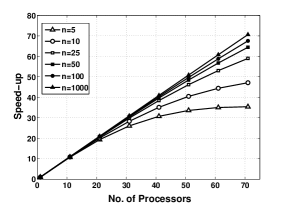
Refer to caption
Figure 4: Theoretical speed-up vs. No. of processors for different system dimensions n𝑛n for l=10𝑙10l=10, dp=2subscript𝑑𝑝2d_{p}=2, da=3subscript𝑑𝑎3d_{a}=3 and d1=d2=4subscript𝑑1subscript𝑑24d_{1}=d_{2}=4, where L+M=53625𝐿𝑀53625L+M=53625

4) Case 4: Synchronization and load balancing

The proposed algorithm is synchronous in that all processors must return values before the centralized step can proceed. However, in the case where we have fewer processors than blocks, some processors may be assigned one block more than other processors. In this case, some processors may remain idle while waiting for the more heavily loaded blocks to complete. In the worst case. this can result in a 50% decrease in speed. We have addressed this issue in the following manner:

  1. 1.

    We allocate almost the same number (±1plus-or-minus1\pm 1) of blocks of the SDP elements C𝐶C and Bisubscript𝐵𝑖B_{i} to all processors, i.e., 𝚏𝚕𝚘𝚘𝚛(L+MN)+1𝚏𝚕𝚘𝚘𝚛𝐿𝑀𝑁1\mathtt{floor}(\frac{L+M}{N})+1 blocks to r𝑟r processors and 𝚏𝚕𝚘𝚘𝚛(L+MN)𝚏𝚕𝚘𝚘𝚛𝐿𝑀𝑁\mathtt{floor}(\frac{L+M}{N}) blocks to the other Nr𝑁𝑟N-r processors, where r𝑟r is the remainder of dividing L+M𝐿𝑀L+M by N𝑁N.

  2. 2.

    We assign the same routine to all of the processors in the Processors steps of Alg. 2.

If L+M𝐿𝑀L+M is a multiple of N𝑁N, then the algorithm assigns the same amount of data, i.e., L+MN𝐿𝑀𝑁\frac{L+M}{N} blocks of C𝐶C and Bisubscript𝐵𝑖B_{i} to each processor. In this case, the processors are perfectly synchronized. If L+M𝐿𝑀L+M is not a multiple of N𝑁N, then according to (83), r𝑟r of N𝑁N processors perform K2n3superscript𝐾2superscript𝑛3K^{2}n^{3} extra operations per iteration. This fraction is 11+𝚏𝚕𝚘𝚘𝚛(L+MN)0.511𝚏𝚕𝚘𝚘𝚛𝐿𝑀𝑁0.5\dfrac{1}{1+\mathtt{floor}(\frac{L+M}{N})}\leq 0.5 of the operations per iteration performed by each of r𝑟r processors. Thus in the worst case, we have a 50% reduction, although this situation is rare. As an example, the load balancing (distribution of data and calculation) for the case of solving an SDP of the size L+M=24𝐿𝑀24L+M=24 using different numbers of available processors N𝑁N is demonstrated in Fig. 5. This figure shows the number of blocks that are allocated to each processor. According to this figure, for N=2,12𝑁212N=2,12 and 24, the processors are well-balanced, whereas for the case where N=18𝑁18N=18, twelve processors perform 50%percent\% fewer calculations.

Refer to caption
Figure 5: The number of blocks of the SDP elements assigned to each processor; An illustration of load balancing

5) Case 5: Communication graph

The communication directed graph of the SDP algorithm (Fig. 6) is static (fixed for all iterations). At each iteration, root sends messages (Δy^Δ^𝑦\Delta\widehat{y} and Δy¯Δ¯𝑦\Delta\overline{y}) to all of the processors and receives messages (λi,k,lsubscript𝜆𝑖𝑘𝑙\lambda_{i,k,l} in (79)) from all of the processors. The adjacency matrix of the communication directed graph is defined as follows. For i=1,,N𝑖1𝑁i=1,\cdots,N and j=1,,N𝑗1𝑁j=1,\cdots,N,

[TG]i,j:={1if(i=1orj=1)and(ij)0Otherwise.assignsubscriptdelimited-[]subscript𝑇𝐺𝑖𝑗cases1if𝑖1or𝑗1and𝑖𝑗0Otherwise[T_{G}]_{i,j}:=\begin{cases}1\quad&\text{if}\;\big{(}i=1\;\text{or}\;j=1\big{)}\;\text{and}\;\big{(}i\neq j\big{)}\\ 0\quad&\text{Otherwise}.\end{cases}\vspace*{-0.2in}
Refer to caption
Figure 6: The communication graph of the SDP algorithm

V TESTING AND VALIDATION

In this section, we present validation data in 4 key areas. First, we present analysis results for a realistic large-scale model of tokamak operation using a discretized PDE model. Next we present accuracy and convergence data and compare our algorithm to the SOS approach. Next, we analyze scalability and speed-up of our algorithm as we increase the number of processors and compare our results to the general-purpose parallel SDP solver SDPARA. Finally, we explore the limits of the algorithm in terms of problems size when implemented on a moderately powerful cluster computer and using a moderate processor allocation on the Blue Gene supercomputer.

1) Example 1: Application to control of a discretized PDE model in fusion research.

The goal of this example is to use the proposed algorithm to solve a real-world stability problem. A simplified model for the poloidal magnetic flux gradient in a Tokamak reactor [56] is

ψx(x,t)t=1μ0a2x(η(x)xx(xψx(x,t)))subscript𝜓𝑥𝑥𝑡𝑡1subscript𝜇0superscript𝑎2𝑥𝜂𝑥𝑥𝑥𝑥subscript𝜓𝑥𝑥𝑡\dfrac{\partial\psi_{x}(x,t)}{\partial t}=\dfrac{1}{\mu_{0}a^{2}}\dfrac{\partial}{\partial x}\left(\dfrac{\eta(x)}{x}\dfrac{\partial}{\partial x}\left(x\psi_{x}(x,t)\right)\right) (91)

with the boundary conditions ψx(0,t)=0subscript𝜓𝑥0𝑡0\psi_{x}(0,t)=0 and ψx(1,t)=0subscript𝜓𝑥1𝑡0\psi_{x}(1,t)=0, where ψxsubscript𝜓𝑥\psi_{x} is the deviation of the flux gradient from a reference flux gradient profile, μ0subscript𝜇0\mu_{0} is the permeability of free space, η(x)𝜂𝑥\eta(x) is the plasma resistivity and a𝑎a is the radius of the last closed magnetic surface (LCMS). To obtain the finite-dimensional state-space representation of the PDE, we discretize the PDE in the spatial domain (0,1)01(0,1). The state-space model is then

ψ˙x(t)=A(η(x))ψx(t),subscript˙𝜓𝑥𝑡𝐴𝜂𝑥subscript𝜓𝑥𝑡\dot{\psi}_{x}(t)=A(\eta(x))\psi_{x}(t), (92)

where A(η(x))N×N𝐴𝜂𝑥superscript𝑁𝑁A(\eta(x))\in\mathbb{R}^{N\times N} has the following non-zero entries.

a11=43μ0Δx2a2(η(x32)x32+2η(x34)x34),subscript𝑎1143subscript𝜇0Δsuperscript𝑥2superscript𝑎2𝜂subscript𝑥32subscript𝑥322𝜂subscript𝑥34subscript𝑥34a_{11}=\dfrac{-4}{3\mu_{0}\Delta x^{2}a^{2}}\left(\dfrac{\eta(x_{\frac{3}{2}})}{x_{\frac{3}{2}}}+\dfrac{2\eta(x_{\frac{3}{4}})}{x_{\frac{3}{4}}}\right),
a12=43μ0Δx2a2(η(x32)x2x32),subscript𝑎1243subscript𝜇0Δsuperscript𝑥2superscript𝑎2𝜂subscript𝑥32subscript𝑥2subscript𝑥32a_{12}=\dfrac{4}{3\mu_{0}\Delta x^{2}a^{2}}\left(\dfrac{\eta(x_{\frac{3}{2}})x_{2}}{x_{\frac{3}{2}}}\right), (93)
aj,j1=1Δx2μ0a2(η(xj12)xj12xj1)forj=2,,N1formulae-sequencesubscript𝑎𝑗𝑗11Δsuperscript𝑥2subscript𝜇0superscript𝑎2𝜂subscript𝑥𝑗12subscript𝑥𝑗12subscript𝑥𝑗1for𝑗2𝑁1a_{j,j-1}=\dfrac{1}{\Delta x^{2}\mu_{0}a^{2}}\left(\dfrac{\eta(x_{j-\frac{1}{2}})}{x_{j-\frac{1}{2}}}x_{j-1}\right)\;\text{for}\;j=2,\cdots,N-1 (94)
aj,j=1Δx2μ0a2(η(xj+12)xj+12+η(xj12)xj12)xjsubscript𝑎𝑗𝑗1Δsuperscript𝑥2subscript𝜇0superscript𝑎2𝜂subscript𝑥𝑗12subscript𝑥𝑗12𝜂subscript𝑥𝑗12subscript𝑥𝑗12subscript𝑥𝑗\displaystyle a_{j,j}=\dfrac{-1}{\Delta x^{2}\mu_{0}a^{2}}\left(\dfrac{\eta(x_{j+\frac{1}{2}})}{x_{j+\frac{1}{2}}}+\dfrac{\eta(x_{j-\frac{1}{2}})}{x_{j-\frac{1}{2}}}\right)x_{j}
forj=2,,N1for𝑗2𝑁1\displaystyle\qquad\qquad\qquad\qquad\qquad\quad\qquad\text{for}\;j=2,\cdots,N-1 (95)
aj,j+1=1Δx2μ0a2(η(xj+12)xj+12xj+1)forj=2,,N1formulae-sequencesubscript𝑎𝑗𝑗11Δsuperscript𝑥2subscript𝜇0superscript𝑎2𝜂subscript𝑥𝑗12subscript𝑥𝑗12subscript𝑥𝑗1for𝑗2𝑁1a_{j,j+1}=\dfrac{1}{\Delta x^{2}\mu_{0}a^{2}}\left(\dfrac{\eta(x_{j+\frac{1}{2}})}{x_{j+\frac{1}{2}}}x_{j+1}\right)\;\text{for}\;j=2,\cdots,N-1 (96)
aN,N1=43Δxμ0a2η(xN12)xN1xN12Δx,subscript𝑎𝑁𝑁143Δ𝑥subscript𝜇0superscript𝑎2𝜂subscript𝑥𝑁12subscript𝑥𝑁1subscript𝑥𝑁12Δ𝑥a_{N,N-1}=\dfrac{4}{3\Delta x\mu_{0}a^{2}}\dfrac{\eta(x_{N-\frac{1}{2}})x_{N-1}}{x_{N-\frac{1}{2}}\Delta x},
aN,N=43Δxμ0a2(2η(xN+14)xNxN+14Δx+η(xN12)xNxN12Δx),subscript𝑎𝑁𝑁43Δ𝑥subscript𝜇0superscript𝑎22𝜂subscript𝑥𝑁14subscript𝑥𝑁subscript𝑥𝑁14Δ𝑥𝜂subscript𝑥𝑁12subscript𝑥𝑁subscript𝑥𝑁12Δ𝑥a_{N,N}=\dfrac{-4}{3\Delta x\mu_{0}a^{2}}\left(\dfrac{2\eta(x_{N+\frac{1}{4}})x_{N}}{x_{N+\frac{1}{4}}\Delta x}+\dfrac{\eta(x_{N-\frac{1}{2}})x_{N}}{x_{N-\frac{1}{2}}\Delta x}\right),\vspace*{-0.05in} (97)

where Δx=1NΔ𝑥1𝑁\Delta x=\dfrac{1}{N} and xj:=(j12)Δxassignsubscript𝑥𝑗𝑗12Δ𝑥x_{j}:=(j-\frac{1}{2})\Delta x.

We discretize the model at N=7𝑁7N=7 points. Typically the η(xk)𝜂subscript𝑥𝑘\eta(x_{k}) are not precisely known (they depend on other state variables), so we substitute for η(xk)𝜂subscript𝑥𝑘\eta(x_{k}) in (92) with η^(xk)+αj^𝜂subscript𝑥𝑘subscript𝛼𝑗\widehat{\eta}(x_{k})+\alpha_{j}, where η^(xk)^𝜂subscript𝑥𝑘\widehat{\eta}(x_{k}) are the nominal values of η(xk)𝜂subscript𝑥𝑘\eta(x_{k}) and αjsubscript𝛼𝑗\alpha_{j} are the uncertain parameters. At xk=0.036,0.143,0.286,0.429,subscript𝑥𝑘0.0360.1430.2860.429x_{k}=0.036,0.143,0.286,0.429, 0.571,0.714,0.857,0.9640.5710.7140.8570.9640.571,0.714,0.857,0.964, we use data from the Tore Supra reactor to estimate the η^(xk)^𝜂subscript𝑥𝑘\widehat{\eta}(x_{k}) as 1.775108,2.703108,5.676108,1.182107,2.058107,3.655107,1.076106,8.4191061.775superscript1082.703superscript1085.676superscript1081.182superscript1072.058superscript1073.655superscript1071.076superscript1068.419superscript1061.775\cdot 10^{-8},2.703\cdot 10^{-8},5.676\cdot 10^{-8},1.182\cdot 10^{-7},2.058\cdot 10^{-7},3.655\cdot 10^{-7},1.076\cdot 10^{-6},8.419\cdot 10^{-6}. The uncertain system is then written as

ψ˙x(t)=A(α)ψx(t),subscript˙𝜓𝑥𝑡𝐴𝛼subscript𝜓𝑥𝑡\dot{\psi}_{x}(t)=A(\alpha)\psi_{x}(t),\vspace*{-0.05in} (98)

where A𝐴A is affine, A(α)=A0+i=18Aiαi𝐴𝛼subscript𝐴0superscriptsubscript𝑖18subscript𝐴𝑖subscript𝛼𝑖A(\alpha)=A_{0}+\sum_{i=1}^{8}A_{i}\alpha_{i} (the Aisubscript𝐴𝑖A_{i} are omitted for the sake of brevity). For a given ρ𝜌\rho, we restrict the uncertain parameters αjsubscript𝛼𝑗\alpha_{j} to Sρsubscript𝑆𝜌S_{\rho}, defined as

Sρ:={α8:i=18αi=6|ρ|,|ρ|αi|ρ|},assignsubscript𝑆𝜌conditional-set𝛼superscript8formulae-sequencesuperscriptsubscript𝑖18subscript𝛼𝑖6𝜌𝜌subscript𝛼𝑖𝜌S_{\rho}:=\{\alpha\in\mathbb{R}^{8}:\sum_{i=1}^{8}\alpha_{i}=-6|\rho|,-|\rho|\leq\alpha_{i}\leq|\rho|\},\vspace*{-0.05in} (99)

which is a simplex translated to the origin. We would like to determine the maximum value of ρ𝜌\rho such that the system is stable by solving the following optimization problem.

maxρ𝜌\max\quad\rho\vspace*{-0.05in}
s.t.System (98) is stable for allαSρ.s.t.System (98) is stable for all𝛼subscript𝑆𝜌\hskip 36.135pt\text{s.t.}\quad\text{System~{}\eqref{eq:discrete_uncertain} is stable for all}\;\alpha\in S_{\rho}.\vspace*{-0.05in} (100)

To represent Sρsubscript𝑆𝜌S_{\rho} using the standard unit simplex defined in (7), we define the invertible map g:Δ8Sρ:𝑔subscriptΔ8subscript𝑆𝜌g:\Delta_{8}\rightarrow S_{\rho} as

g(α)=[g1(α)g8(α)],gi(α):=2|ρ|(αi0.5).formulae-sequence𝑔𝛼matrixsubscript𝑔1𝛼subscript𝑔8𝛼assignsubscript𝑔𝑖𝛼2𝜌subscript𝛼𝑖0.5g(\alpha)=\begin{bmatrix}g_{1}(\alpha)&\cdots&g_{8}(\alpha)\end{bmatrix},\;g_{i}(\alpha):=2|\rho|(\alpha_{i}-0.5).\vspace*{-0.025in} (101)

Then, if we let A(α)=A(g(α))superscript𝐴𝛼𝐴𝑔𝛼A^{\prime}(\alpha)=A(g(\alpha)), since g𝑔g is one-to-one,

{A(α):αSρ}={A(g(α)):αΔ8}={A(α):αΔ8}.conditional-set𝐴superscript𝛼superscript𝛼subscript𝑆𝜌conditional-set𝐴𝑔𝛼𝛼subscriptΔ8conditional-setsuperscript𝐴𝛼𝛼subscriptΔ8\{A(\alpha^{\prime}):\alpha^{\prime}\in S_{\rho}\}=\{A(g(\alpha)):\alpha\in\Delta_{8}\}=\{A^{\prime}(\alpha):\alpha\in\Delta_{8}\}.\vspace*{-0.05in}

Thus stability of ψ˙x(t)=A(α)ψx(t), for all αΔlformulae-sequencesubscript˙𝜓𝑥𝑡superscript𝐴𝛼subscript𝜓𝑥𝑡 for all 𝛼subscriptΔ𝑙\dot{\psi}_{x}(t)=A^{\prime}(\alpha)\psi_{x}(t),\text{ for all }\alpha\in\Delta_{l} is equivalent to stability of Equation (98) for all αSρ𝛼subscript𝑆𝜌\alpha\in S_{\rho}.

We solve the optimization problem in (100) using bisection. For each trial value of ρ𝜌\rho, we use the proposed parallel SDP solver to solve the associated SDP obtained by the parallel set-up algorithm. The SDP problems have 224 constraints with the primal variable X1092×1092𝑋superscript10921092X\in\mathbb{R}^{1092\times 1092}. The normalized maximum value of ρ𝜌\rho is found to be 0.00190.00190.0019. In this particular example, the optimal value of ρ𝜌\rho does not change with the degrees of P(α)𝑃𝛼P(\alpha) and Polya’s exponents d1subscript𝑑1d_{1} and d2subscript𝑑2d_{2}, primarily because the model is affine.

The SDPs are constructed and solved on a parallel Linux-based cluster Cosmea at Argonne National Laboratory. Fig. 7 shows the algorithm speed-up vs. the number of processors. Note that solving this problem by SOSTOOLS [21] on the same machine is impossible due to the lack of unallocated memory.
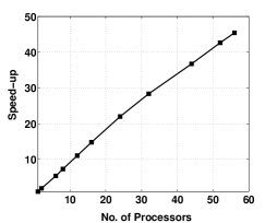
Refer to caption
Figure 7: Speed-up of set-up and SDP algorithms vs. number of processors for a discretized model of magnetic flux in Tokamak

2) Example 2: Accuracy and Convergence

The goal of this example is to investigate the effect of the degree of P(α)𝑃𝛼P(\alpha), dpsubscript𝑑𝑝d_{p}, and the Polya’s exponents, d1,d2subscript𝑑1subscript𝑑2d_{1},d_{2} on the accuracy of the algorithm. Given a computer with fixed amount of RAM, we compare the accuracy of the proposed algorithm with SOS algorithm. Consider the system x˙(t)=A(α)x(t)˙𝑥𝑡𝐴𝛼𝑥𝑡\dot{x}(t)=A(\alpha)x(t) where A𝐴A is a polynomial degree 3 defined as

A(α)=A1α13+A2α12α2+A3α1α2α3+A4α1α32+A5α23+A6α33𝐴𝛼subscript𝐴1superscriptsubscript𝛼13subscript𝐴2superscriptsubscript𝛼12subscript𝛼2subscript𝐴3subscript𝛼1subscript𝛼2subscript𝛼3subscript𝐴4subscript𝛼1superscriptsubscript𝛼32subscript𝐴5superscriptsubscript𝛼23subscript𝐴6superscriptsubscript𝛼33A(\alpha)=A_{1}\alpha_{1}^{3}+A_{2}\alpha_{1}^{2}\alpha_{2}+A_{3}\alpha_{1}\alpha_{2}\alpha_{3}+A_{4}\alpha_{1}\alpha_{3}^{2}+A_{5}\alpha_{2}^{3}+A_{6}\alpha_{3}^{3}\vspace*{-0.1in} (102)

with the constraint

αSL:={α3:i=13αi=2L+1,Lαi1}𝛼subscript𝑆𝐿assignconditional-set𝛼superscript3formulae-sequencesuperscriptsubscript𝑖13subscript𝛼𝑖2𝐿1𝐿subscript𝛼𝑖1\alpha\in S_{L}:=\left\{\alpha\in\mathbb{R}^{3}:\sum_{i=1}^{3}\alpha_{i}=2L+1,L\leq\alpha_{i}\leq 1\right\}
A1=[0.610.560.4020.480.5500.6711.010.9180.029],A2=[0.4840.861.50.7320.8410.1260.6850.3050.106]formulae-sequencesubscript𝐴1delimited-[]0.610.560.4020.480.5500.6711.010.9180.029subscript𝐴2delimited-[]0.4840.861.50.7320.8410.1260.6850.3050.106\displaystyle A_{1}=\left[\begin{array}[]{ccc}-0.61&-0.56&0.402\\ -0.48&-0.550&0.671\\ -1.01&-0.918&0.029\end{array}\right],\hskip 7.22743ptA_{2}=\left[\begin{array}[]{ccc}-0.484&-0.86&1.5\\ -0.732&-0.841&-0.126\\ 0.685&0.305&0.106\end{array}\right]
A3=[0.3570.3440.6610.2100.5050.5880.2680.4870.846],A4=[0.8810.4360.2280.5030.8120.2490.0120.5420.536]formulae-sequencesubscript𝐴3delimited-[]0.3570.3440.6610.2100.5050.5880.2680.4870.846subscript𝐴4delimited-[]0.8810.4360.2280.5030.8120.2490.0120.5420.536\displaystyle A_{3}=\left[\begin{array}[]{ccc}-0.357&0.344&-0.661\\ -0.210&-0.505&0.588\\ 0.268&0.487&-0.846\\ \end{array}\right],A_{4}=\left[\begin{array}[]{ccc}-0.881&-0.436&0.228\\ 0.503&-0.812&0.249\\ -0.012&0.542&-0.536\end{array}\right]
A5=[0.7030.2980.1780.4020.7610.3000.0100.4610.588],A6=[0.2010.1820.5570.8030.4120.2030.4400.0110.881]formulae-sequencesubscript𝐴5delimited-[]0.7030.2980.1780.4020.7610.3000.0100.4610.588subscript𝐴6delimited-[]0.2010.1820.5570.8030.4120.2030.4400.0110.881\displaystyle A_{5}=\left[\begin{array}[]{ccc}-0.703&-0.298&-0.178\\ 0.402&-0.761&-0.300\\ -0.010&0.461&-0.588\end{array}\right],A_{6}=\left[\begin{array}[]{ccc}-0.201&-0.182&-0.557\\ 0.803&-0.412&-0.203\\ -0.440&0.011&-0.881\end{array}\right]

Defining g𝑔g as in Example 1, the problem is

minL𝐿\min\quad L\vspace*{-0.1in}
s.t.x˙(t)=A(g(α))x(t)is stable for allαΔ3.s.t.˙𝑥𝑡𝐴𝑔𝛼𝑥𝑡is stable for all𝛼subscriptΔ3\hskip 14.45377pt\text{s.t.}\quad\dot{x}(t)=A(g(\alpha))x(t)\;\text{is stable for all}\;\alpha\in\Delta_{3}.\vspace*{-0.1in} (103)

Using bisection in L𝐿L, as in Example 1, we varied the parameters dpsubscript𝑑𝑝d_{p}, d1subscript𝑑1d_{1} and d2subscript𝑑2d_{2}. The cluster computer Karlin at the Illinois Institute of Technology with 24 Gbytes/node of RAM (216 Gbytes total memory) was used to run our algorithm. The upper bounds on the optimal L𝐿L are shown in Fig. 9 in terms of d1subscript𝑑1d_{1} and d2subscript𝑑2d_{2} and for different dpsubscript𝑑𝑝d_{p}. Considering the optimal value of L𝐿L to be Lopt=0.111subscript𝐿opt0.111L_{\text{opt}}=-0.111, Fig. 9 shows how increasing dpsubscript𝑑𝑝d_{p} and/or d1,d2subscript𝑑1subscript𝑑2d_{1},d_{2} - when they are still relatively small - improves the accuracy of the algorithm. Fig. 9 demonstrates how the error in our upper bound for Loptsubscript𝐿optL_{\text{opt}} decreases by increasing dpsubscript𝑑𝑝d_{p} and/or d1,d2subscript𝑑1subscript𝑑2d_{1},d_{2}.

For comparison, we solved the same stability problem using the SOS algorithm [21] using only a single node of the same cluster computer and 24 Gbytes of RAM. We used the Positivstellensatz approach based on [57] to impose the constraints i=13αi=2L+1superscriptsubscript𝑖13subscript𝛼𝑖2𝐿1\sum_{i=1}^{3}\alpha_{i}=2L+1 and Lαi1𝐿subscript𝛼𝑖1L\leq\alpha_{i}\leq 1. Table I shows the upper bounds on L𝐿L given by the SOS algorithm using different degrees for x𝑥x and α𝛼\alpha. By considering a Lyapunov function of degree two in x𝑥x and degree one in α𝛼\alpha, the SOS algorithm gives 0.1020.102-0.102 as the upper bound on Loptsubscript𝐿𝑜𝑝𝑡L_{opt} as compared with our value of 0.1110.111-0.111. Increasing the degree of α𝛼\alpha in the Lyapunov function beyond degree two resulted in a failure due to lack of memory. Note that while relevant, this comparison may not be entirely fair as the SOS algorithm has not been decentralized and it can handle global nonlinear stability problems, which our algorithm cannot.

TABLE I: Upper bounds found for Loptsubscript𝐿𝑜𝑝𝑡L_{opt} by SOS algorithm using different degrees for x𝑥x and α𝛼\alpha (inf: infeasible, O.M.: Out of Memory)
Degree in x𝑥x Degree in α𝛼\alpha 0 1 2
1 inf. inf. inf.
2 inf. -0.102 O.M.
3 inf. O.M. O.M.
Refer to caption
Figure 8: Upper bound on optimal L𝐿L vs. Polya’s exponents d1subscript𝑑1d_{1} and d2subscript𝑑2d_{2}, for different degrees of P(α)𝑃𝛼P(\alpha). (d1=d2subscript𝑑1subscript𝑑2d_{1}=d_{2}).
Refer to caption
Figure 9: Error of the approximation for the optimal value of L𝐿L vs. degrees of P(α)𝑃𝛼P(\alpha), for different Polya’s exponents

3) Example 3: Speed-up

In this example we evaluate the efficiency of the algorithm in using additional processors to decrease computation time. As mentioned in Section IV-D on computational complexity, the measure of this efficiency is termed speed-up and in Case 3, we gave a formula for this number. To evaluate the true speed-up, we first ran the set-up algorithm on the Blue Gene supercomputer at Argonne National Laboratory using three random linear systems with different state-space dimensions and numbers of uncertain parameters. Fig. 11 shows a log-log plot of the computation time of the set-up algorithm vs. the number of processors. As can be seen, the scalability of the algorithm is practically ideal for several different state-space dimensions and numbers of uncertain parameters.

To evaluate the speed-up of the SDP portion of the algorithm, we solved three random SDP problems with different dimensions using the Karlin cluster computer. Fig. 11 gives a log-log plot of the computation time of the SDP algorithm vs. the number of processors for three different dimensions of the primal variable X𝑋X and the dual variable y𝑦y. As indicated in the figure, the three dimensions of the primal variable X𝑋X are 200, 385200385200,\;385 and 1092, and the dimensions of the dual variable y𝑦y are K=50, 90𝐾5090K=50,\;90 and 224, respectively. In all cases, dp=2subscript𝑑𝑝2d_{p}=2 and d1=d2=1subscript𝑑1subscript𝑑21d_{1}=d_{2}=1. The linearity of the Time vs. Number of Processors curves in all three cases demonstrates the scalability of the SDP algorithm.

For comparison, we plot the speed-up of our algorithm vs. that of the general-purpose parallel SDP solver SDPARA 7.3.1 as illustrated in Fig. 12. Although similar for a small number of processors, for a larger number of processors, SDPARA saturates, while our algorithm remains approximately linear.
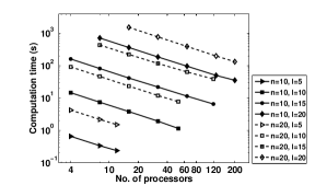
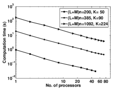
Refer to caption
Figure 10: Computation time of the parallel set-up algorithm vs. number of processors for different dimensions of linear system n𝑛n and numbers of uncertain parameters l𝑙l- executed on Blue Gene supercomputer of Argonne National Labratory
Refer to caption
Figure 11: Computation time of the parallel SDP algorithm vs. number of processors for different dimensions of primal variable (L+M)n𝐿𝑀𝑛(L+M)n and of dual variable K𝐾K- executed on Karlin cluster computer of Illinois Institute of Technology
Refer to caption
Figure 12: Comparison between the speed-up of the present SDP solver and SDPARA 7.3.1, executed on Karlin cluster computer

4) Example 4: Max state-space and parameter dimensions for a 9-node Linux cluster computer

The goal of this example is to show that given moderate computational resources, the proposed decentralized algorithms can solve robust stability problems for systems with 100+ states. We used the Karlin cluster computer with 24 Gbytes/node RAM and nine nodes. We ran the set-up and SDP algorithms to solve the robust stability problem with dimension n𝑛n and l𝑙l uncertain parameters on one and nine nodes of Karlin cluster computer. Thus the total memory access was thus 24 Gig and 216 Gig, respectively. Using trial and error, for different n𝑛n and d1,d2subscript𝑑1subscript𝑑2d_{1},d_{2} we found the largest l𝑙l for which the algorithms do not terminate due to insufficient memory (Fig. 13). In all of the runs da=dp=1subscript𝑑𝑎subscript𝑑𝑝1d_{a}=d_{p}=1. Fig. 13 shows that by using 216 Gbytes of RAM, the algorithms can solve the stability problem of size n=100𝑛100n=100 with 4 uncertain parameters in d1=d2=1subscript𝑑1subscript𝑑21d_{1}=d_{2}=1 Polya’s iteration and with 3 uncertain parameters in d1=d2=4subscript𝑑1subscript𝑑24d_{1}=d_{2}=4 Polya’s iterations.

Refer to caption
Refer to caption
Figure 13: Largest number of uncertain parameters of n𝑛n-dimensional systems for which the set-up algorithm (Left) and SDP solver (Right) can solve the robust stability problem of the system using 24 and 216 Gig of RAM

VI Conclusion

In this paper, we have presented a cluster-computing and supercomputing approach to stability analysis of large-scale linear systems of the form x˙(t)=A(α)x(t)˙𝑥𝑡𝐴𝛼𝑥𝑡\dot{x}(t)=A(\alpha)x(t) where A𝐴A is polynomial, αΔll𝛼subscriptΔ𝑙superscript𝑙\alpha\in\Delta_{l}\subset\mathbb{R}^{l} and xn𝑥superscript𝑛x\in\mathbb{R}^{n} and where n100𝑛100n\cong 100 or α10𝛼10\alpha\cong 10. The approach is based on mapping the structure of the LMI conditions associated with Polya’s theorem to a decentralized computing environment. We have shown that for a sufficient number of processors, the proposed algorithm can solve the NP-hard robust stability problem with the same per-core computation cost as solving the Lyapunov inequality for a system with no parametric uncertainty. Theoretical and experimental results verify near-perfect scalability and speed-up for up to 200 processors. Moreover, numerical examples demonstrate the ability of the algorithm to perform robust analysis of systems with 100+ states and several uncertain parameters using a simple 9-node Linux cluster computer. We have also argued that our algorithms can also be extended to solve nonlinear stability analysis and robust controller synthesis problems, although this is left for future work.

References

  • [1] S. Gugercin and A. Antoulas, “A survey of model reduction by balanced truncation and some new results,” International Journal of Control, vol. 77, no. 8, pp. 748–766, 2004.
  • [2] J. Ackermann, A. Bartlett, D. Kaesbauer, W. Sienel, and R. Steinhauser, Robust Control: Systems with Uncertain Physical Parameters. Secaucus, NJ, USA: Springer-Verlag New York, Inc., 2001.
  • [3] S. P. Bhattacharyya, H. Chapellat, and L. H. Keel, Robust Control: The Parametric Approach. Prentice Hall, 1995.
  • [4] M. Green and D. J. N. Limebeer, Linear robust control. Upper Saddle River, NJ, USA: Prentice-Hall, Inc., 1995.
  • [5] K. Zhou and J. Doyle, Essentials of Robust Control. Prentice Hall, 1998.
  • [6] V. Blondel and J. Tsitsiklis, “A survey of computational complexity results in systems and control,” Automatica, vol. 36, no. 9, pp. 1249–1274, 2000.
  • [7] A. Nemirovskii, “Several NP-hard problems arising in robust stability analysis,” Mathematics of Control, Signals, and Systems (MCSS), vol. 6, no. 2, pp. 99–105, 1993.
  • [8] D. Walker and J. Dongarra, “Mpi: a standard message passing interface,” Supercomputer, vol. 12, pp. 56–68, 1996.
  • [9] A. Packard and J. Doyle, “Quadratic stability with real and complex perturbations,” IEEE Transactions on Automatic Control, vol. 35, pp. 198–201, Feb 1990.
  • [10] B. R. Barmish and C. L. DeMarco, “A new method for improvement of robustness bounds for linear state equations,” in Proceedings Conf. Inform. Sci. Syst. Princeton University, 1986.
  • [11] P. Gahinet, P. Apkarian, and M. Chilali, “Affine parameter-dependent lyapunov functions and real parametric uncertainty,” IEEE Transactions on Automatic Control, vol. 41, pp. 436–442, Mar 1996.
  • [12] R. C. L. F. Oliveira and P. L. D. Peres, “Stability of polytopes of matrices via affine parameter-dependent Lyapunov functions: Asymptotically exact LMI conditions,” Linear Algebra Appl., vol. 405, pp. 209–228, Aug 2005.
  • [13] R. C. L. F. Oliveira and P. L. D. Peres, “A less conservative LMI condition for the robust stability of discrete-time uncertain systems,” Syst. Control Lett., vol. 43, pp. 371–378, Aug 2001.
  • [14] D. Ramos and P. Peres, “An LMI approach to compute robust stability domains for uncertain linear systems,” Proceedings of the American Control Conference, Jun 2001.
  • [15] P. A. Bliman, “An existence result for polynomial solutions of parameter dependent LMIs,” Systems & Control Letters, no. 3-4, pp. 165–169, 2004.
  • [16] M. Peet, “Exponentially stable nonlinear systems have polynomial lyapunov functions on bounded regions,” Automatic Control, IEEE Transactions on, vol. 54, no. 5, pp. 979–987, 2009.
  • [17] A. Ben-Tal and A. Nemirovski, “Robust convex optimization,” Math. Operat. Res., vol. 23, no. 4, pp. 769–805, 1998.
  • [18] P. A. Bliman, “A convex approach to robust stability for linear systems with uncertain scalar parameters,” SIAM J. Control Optim, vol. 42, no. 3-4, pp. 2016–2042, 2004.
  • [19] X. Zhang and P. Tsiotras, “Parameter-dependent lyapunov functions for stability analysis of LTI parameter dependent systems,” pp. 5168–5173, in Proceedings of the IEEE 42nd Conference on Decision and Control, 2003.
  • [20] X. Zhang, P. Tsiotras, and P. A. Bliman, “Multi-parameter dependent lyapunov functions for the stability analysis of parameter-dependent LTI systems,” pp. 1263–1268, in Proceedings of IEEE International Symposium on, Mediterrean Conference on Control and Automation, 2005.
  • [21] S. Prajna, A. Papachristodoulou, and P. A. Parrilo, “Introducing SOSTOOLS: a general purpose sum of squares programming solver,” Proceedings of IEEE Conference on Decision and Control, 2002.
  • [22] D. Henrion and J. B. Lassere, “Gloptipoly: Global optimization over polynomials with Matlab and SeDuMi,” Proceedings of IEEE Conference on Decision and Control, Mar 2003.
  • [23] C. W. Scherer and C. W. J. Hol, “Matrix sum-of squares relaxations for robust semi-definite programs,” Math. programming Ser. B, vol. 107, no. 1-2, pp. 189–211, 2006.
  • [24] G. Chesi, A. Garulli, A. Tesi, and A. Vicino, “Polynomially parameter-dependent lyapunov functions for robust stability of polytopic systems: an LMI approach,” IEEE Transactions on Automatic Control, vol. 50, pp. 365–370, Mar 2005.
  • [25] R. C. L. F. Oliveira and P. L. D. Peres, “Parameter-dependent LMIs in robust analysis: Characterization of homogeneous polynomially parameter-dependent solutions via LMI relaxations,” IEEE Transactions on Automatic Control, vol. 52, pp. 1334–1340, Jul 2007.
  • [26] R. C. L. F. Oliveira, P.-A. Bliman, and P. L. D. Peres, “Robust LMIs with parameters in multi-simplex: Existence of solutions and applications,” pp. 2226–2231, Proceedings of IEEE Conference on Decision and Control, 2008.
  • [27] B. Borchers and J. G. Young, “Implementation of a primal dual method for SDP on a shared memory parallel architecture,” Computational Optimization and Applications, vol. 37, no. 3, pp. 355–369, 2007.
  • [28] M. Yamashita, K. Fujisawa, and M. Kojima, “SDPARA: Semidefinite programming algorithm parallel version,” Parallel Computing, vol. 29, pp. 1053–1067, 2003.
  • [29] G. M. Amdahl, “Validity of the single processor approach to achieving large-scale computing capabilities,” No. 30, pp. 483–485, AFIPS Conference Proceedings, 1967.
  • [30] L. Kalé, B. Ramkumar, A. Sinha, and A. Gursoy, “The charm parallel programming language and system: Part i–description of language features,” Parallel Programming Laboratory Technical Report No. 95-02, 1994.
  • [31] S. Deitz, High-level programming language abstractions for advanced and dynamic parallel computations. PhD thesis, Computer Science and Engineering Department, University of Washington, 2005.
  • [32] K. Gatermann and P. Parrilo, “Symmetry groups, semidefinite programs, and sums of squares,” Journal of Pure and Applied Algebra, vol. 192, no. 1, pp. 95–128, 2004.
  • [33] P. Parrilo, “Exploiting algebraic structure in sum of squares programs,” Positive polynomials in control, pp. 580–580, 2005.
  • [34] S. Kim, M. Kojima, and H. Waki, “Generalized lagrangian duals and sums of squares relaxations of sparse polynomial optimization problems,” SIAM Journal on Optimization, vol. 15, no. 3, pp. 697–719, 2005.
  • [35] H. Waki, S. Kim, M. Kojima, M. Muramatsu, and H. Sugimoto, “Algorithm 883: Sparsepop—a sparse semidefinite programming relaxation of polynomial optimization problems,” ACM Trans. Math. Softw., vol. 35, no. 2, 2008.
  • [36] D. Cox, J. Little, and D. O’Shea, Ideals, varieties, and algorithms: an introduction to computational algebraic geometry and commutative algebra, vol. 10. Springer Verlag, 2007.
  • [37] B. Buchberger and F. Winkler, Gröbner bases and applications, vol. 251. Cambridge Univ Pr, 1998.
  • [38] M. M. Peet and Y. V. Peet, “A parallel-computing solution for optimization of polynomials,” Proceedings of the American Control Conference, Jun-Jul 2010.
  • [39] E. Scheinerman, Mathematics: A Discrete Introduction, Second Edition. Thomson Brooks/Cole Publishing Co., United States, 2005.
  • [40] G. Hardy, J. E. Littlewood, and G. Pólya, Inequalities. Cambridge University Press, 1934.
  • [41] M. Castle, V. Powers, and B. Reznick, “A quantitative polya’s theorem with zeros,” Effective Methods in Algebraic Geometry, vol. 44, no. 9, pp. 1285–1290, 2009.
  • [42] P. Gahinet and P. Apkarian, “A linear matrix inequality approach to H infinity control,” International Journal of Robust and Nonlinear Control, vol. 4, pp. 421–448, 1994.
  • [43] G. Dullerud and F. Paganini, A course in robust control theory, vol. 6. Springer New York, 2000.
  • [44] S. J. Benson, “DSDP3: Dual scaling algorithm for general positive semidefinite programs,” Technical Report. ANL/MCS-P851-1000, Argonne National Labs, 2001.
  • [45] S. J. Benson, Y. Ye, and X. Zhang, “Solving large-scale sparse semidefinite programs for combinatorial optimization,” SIAM Journal on Optimization, vol. 10, pp. 443–461, 1998.
  • [46] F. Alizadeh, J. A. Haeberly, and M. Overton, “Primal-dual interior-point methods for semidefinite programming: Convergence rates, stability and numerical results,” SIAM Journal on Optimization, vol. 8, no. 3, pp. 746–768, 1998.
  • [47] R. D. C. Monteiro, “Primal-dual path following algorithms for semidefinite programming,” SIAM Journal on Optimization, vol. 7, no. 3, 1997.
  • [48] C. Helmberg, F. R. R. J. Vanderbei, and H. Wolkovicz, “An interior-point method for semidefinite programming,” SIAM Journal on Optimization, vol. 6, pp. 342–361, 1996.
  • [49] C. Helmberg and F. Rendl, “A spectral bundle method for semidefinite programming,” SIAM Journal on Optimization, vol. 10, no. 3, pp. 673–696, 2000.
  • [50] K. K. Sivaramakrishnan, “A parallel interior point decomposition algorithm for block angular semidefinite programs,” Comput. Optim. Appl., vol. 46, no. 1, pp. 1–29, 2010.
  • [51] M. Nayakkankuppam, “Solving large-scale semidefinite programs in parallel,” Mathematical programming, vol. 109, no. 2, pp. 477–504, 2007.
  • [52] M. L. O. F. Alizadeh, J. P. A. Haeberly, “Primal-dual interior-point methods for semidefinite programming,” Math Programming Symposium, Ann Arbor 1994.
  • [53] F. Alizadeh, J. Haeberly, and M. Overton, “Primal-dual interior-point methods for semidefinite programming: convergence rates, stability and numerical results,” SIAM Journal on Optimization, vol. 8, no. 3, pp. 746–768, 1998.
  • [54] R. Greenlaw, H. Hoover, and W. Ruzzo, Limits to parallel computation: P-completeness theory. Oxford University Press, USA, 1995.
  • [55] J. Sturm, “Using sedumi 1.02, a MATLAB toolbox for optimization over symmetric cones,” Optimization Methods and Software, vol. 11-12, pp. 625–653, 1999.
  • [56] E. Witrant, E. Joffrin, S. Brémont, G. Giruzzi, D. Mazon, O. Barana, and P. Moreau, “A control-oriented model of the current profile in tokamak plasma,” Plasma Physics and Controlled Fusion, vol. 49, pp. 1075–1105, 2007.
  • [57] G. Stengle, “A nullstellensatz and a positivstellensatz in semialgebraic geometry,” Mathematische Annalen, vol. 207, no. 2, pp. 87–97, 1973.
[Uncaptioned image] Reza Kamyar received the B.S. and M.S in aerospace engineering from Sharif University of Technology, Tehran, Iran in 2008, and 2010. He is currently a Ph.D student in the department of mechanical engineering of Arizona State University, Tempe, Arizona. He is a research assistant with Cybernetic Systems and Controls Laboratory (CSCL) in the School for Engineering of Matter, Transport and Energy (SEMTE) at Arizona State University. His research focuses on the development of decentralized algorithms applied to the problems of stability and control of large-scale complex systems.
[Uncaptioned image] Matthew M. Peet received the B.S. degrees in physics and in aerospace engineering from the University of Texas at Austin in 1999 and the M.S. and Ph.D. degrees in aeronautics and astronautics from Stanford University, Stanford, CA, in 2001 and 2006, respectively. He was a Postdoctoral Fellow at the National Institute for Research in Computer Science and Control (INRIA), Paris, France, from 2006 to 2008, where he worked in the SISYPHE and BANG groups. He was an Assistant Professor of Aerospace Engineering in the Mechanical, Materials, and Aerospace Engineering Department, Illinois Institute of Technology, Chicago, from 2008 to 2012. He is currently an Assistant Professor of Aerospace Engineering in the School for the Engineering of Matter, Transport, and Energy at Arizona State University, Tempe, and Director of the Cybernetic Systems and Controls Laboratory. His research interests are in the role of computation as it is applied to the understanding and control of complex and large-scale systems. Applications include fusion energy and immunology. Dr. Peet received an NSF CAREER award in 2011.
[Uncaptioned image] Yulia Peet is an Assistant Professor of Mechanical and Aerospace Engineering at the School for Engineering of Matter, Transport and Energy at Arizona State University. Her Ph.D. degree is in Aeronautics and Astronautics from Stanford (2006), M.S. in Aerospace Engineering (1999) and B.S. in Applied Mathematics and Physics (1997) from Moscow Institute of Physics and Technology in Russia. Her previous appointments include a postdoctoral position at the University of Pierre and Marie Curie in Paris in 2006-2008, and a dual appointment as an NSF research and teaching fellow at Northwestern University and assistant computational scientist at the Mathematics and Computer Science Division at Argonne National Laboratory in 2009-2012.