Cosmological Leverage from the Matter Power Spectrum in the Presence of Baryon and Nonlinear Effects

Abstract

We investigate how the use of higher wavenumbers (smaller scales) in the galaxy clustering power spectrum influences cosmological constraints. We take into account uncertainties from nonlinear density fluctuations, (scale dependent) galaxy bias, and baryonic effects. Allowing for substantially model independent uncertainties through separate fit parameters in each wavenumber bin that also allow for the redshift evolution, we quantify strong gains in dark energy and neutrino mass leverage with increasing maximum wavenumber, despite marginalizing over numerous (up to 125) extra fit parameters. The leverage is due to not only an increased number of modes but, more significantly, breaking of degeneracies beyond the linear regime.

I Introduction

The statistical pattern of large scale structure in the universe contains a wealth of information on the cosmological parameters, including the nature of dark energy and the sum of neutrino masses. While the linear density perturbation power spectrum of dark matter can be related to the cosmological model in a straightforward manner, the observational data involves several complicating effects. We would like to use not only fully linear modes but the more numerous higher wavenumber modes where nonlinear effects appear; indeed the nonlinear regime contains not just more modes but distinct cosmological leverage.

On these smaller scales, our understanding of the cosmological dependence is imperfect, while the statistical precision of large volume surveys can reach the subpercent level. Moreover, since we observe the light from galaxies, the mapping from dark matter predictions to data involves the galaxy bias factor, expected to be scale dependent beyond the linear regime. Finally, since galaxies contain dissipative baryons, various dynamical and feedback mechanisms not present for pure dark matter will alter the power spectrum.

These nonlinearity, bias, and baryon effects can be addressed in a number of ways, such as perturbation theory, the halo model formalism, and advanced N-body and hydrodynamic computational simulations, with varying levels of success. Considerable literature exists on these issues; for a selection see White (2004); Zhan and Knox (2004); Huterer and Takada (2005); Huterer and White (2005); Hagan et al. (2005); Jing et al. (2006); Rudd et al. (2008); Zentner et al. (2008); Hearin et al. (2012); Zentner et al. (2013). For some recent work, especially regarding baryonic effects on the weak lensing shear power spectrum, see Natarajan et al. (2014); Eifler et al. (2014); Harnois-Déraps et al. (2014); Mohammed et al. (2014). The further we extend to higher wavenumbers, the less certain we are of having captured all the necessary physics inputs, especially for the range of cosmologies to be examined. One approach is simply to cut out the scales beyond the (quasi)linear regime, using only wavenumbers up to some low $k_{\rm max}$. This severely restricts the information used to a small fraction of the data provided by the survey. An alternate approach is to focus on the cosmological information and marginalize over the uncertain effects. This uses more of the data, but the key danger here is assuming an improper functional form for the unknown influences and so causing a systematic bias in the cosmological conclusions.

We follow the marginalization approach but in a substantially model independent way, allowing the nonlinearity, galaxy bias, and baryon effects to float freely in bins of wavenumber without imposing a functional form for their scale dependence. This effectively removes the danger of distorting the cosmology results. The question then is whether the degradation in cosmological constraints due to the additional bin fit parameters outweighs the gain from including the further data. We focus on the real space matter power spectrum, for clarity in assessing the cosmological information content as a function of $k_{\rm max}$ and because it is central to a variety of different cosmological probes; it is given by the substantially transverse modes of a spectroscopic galaxy redshift survey, and enters in the angular galaxy power spectrum of photometric surveys and in the weak lensing shear power spectrum.

In Sec. II we describe our method of accounting for the scale and redshift dependence of the uncertain physics beyond the linear regime. We lay out the Fisher analysis approach and galaxy redshift survey characteristics in Sec. III, then examine the behavior of the derived cosmological constraints as a function of $k_{\rm max}$ in Sec. IV. To test the robustness of the model independence, in Sec. V we consider alternative fiducials for the scale and redshift dependence. Appendix A further tests the approach by varying the binning properties. We discuss and summarize the results in Sec. VI.

II Power Spectrum Effects

In the linear density perturbation regime, the real space dark matter power spectrum is readily given by Boltzmann codes such as CAMB Lewis et al. (2000) or CLASS Blas et al. (2011). This can be extended beyond the linear regime through simulations or emulators built on simulations, e.g. Lawrence et al. (2010); Heitmann et al. (2014), or through nonlinear mapping of the linear power spectrum in algorithms such as Halofit Smith et al. (2003) and its variants. Considerable work has recently gone into substantially extending perturbation theory and general wavenumber expansions to higher Fourier wavenumbers $k$, such as through the effective theory of large scale structure (see Senatore and Zaldarriaga (2014) and references therein) or the halo model (e.g. Mohammed and Seljak (2014)). The status of these in accounting accurately for galaxy bias and baryon effects, over a range of cosmologies, is not yet clear though interesting progress is being made.

Here we consider a phenomenological approach that does not rely on understanding fully the cosmological dependence of internal halo distributions or baryonic feedback. We write the power spectrum as

$$P_{X}(k,z)=b_{X}^{2}(k,z)\,P_{\rm model}(k,z)\,M_{\rm baryon}(k,z)\ ,$$ (1)

where $P_{\rm model}$ is some model for the (nonlinear) power spectrum whose cosmological dependence is well defined. This is multiplied by a factor $b_{X}^{2}$ describing the possibly scale dependent galaxy bias for some galaxy population $X$, and another function $M_{\rm baryon}$ dealing with baryonic effects. The separability of the factors is not essential, only for illustrative purposes.

Uncertainties in the bias factor will be degenerate with those in the baryonic factor (unless specific functional forms are assumed), so we can absorb these both into the same factor, writing

$$P_{X}(k,z)=b_{X,{\rm fid}}^{2}(z)\,P_{\rm model}(k,z)\,M(k,z)\ .$$ (2)

Thus the uncertainties due to galaxy bias, nonlinearities, and baryonic effects are represented by the function $M(k,z)$. For compactness, we call $M$ the BNB factor, referring to all three sources of uncertainty. We will then marginalize over this and study the effect on the cosmological information extracted from the data.

Our best guess, baseline dark matter power spectrum is $P_{\rm model}$ and this includes all the cosmological parameter dependence we will use. While $M$ may have further cosmological dependence, this will be lost in the marginalization, reducing the statistical leverage but guarding against systematic bias. We adopt for $P_{\rm model}$ the revised Halofit form of Takahashi et al. (2012), updating the original Smith et al. (2003). Note that in the CAMB and CLASS versions from March 2014 and later this also includes the neutrino mass effects from Bird et al. (2012).

To keep explicit the galaxy population dependence we retain a fiducial galaxy bias factor

$$b_{X,{\rm fid}}(z)=b^{0}_{X,{\rm fid}}\,\frac{D_{\rm fid}(z=0)}{D_{\rm fid}(z)}\ ,$$ (3)

where $D_{\rm fid}$ is the growth factor for some fiducial cosmology. All deviations in the galaxy bias from this form, including scale dependence, enter in $M$ (as do deviations from the Halofit prescription for nonlinearity, and baryonic effects, i.e. the BNB effects).

To keep $M(k,z)$ as general as possible to account for these uncertainties, we allow it to float freely in bins of wavenumber $k$, so that the data determines its form and amplitude. This approach worked well in exploration of the anisotropic, redshift space power spectrum uncertainties (without baryon or scale dependent bias effects) and its cosmological leverage in Linder and Samsing (2013). The redshift dependence of $M$ should be reasonably smooth as galaxy bias, excess nonlinearity, and baryonic effects develop on a roughly Hubble time scale.

Our prescription is therefore

$$M(k,z)=(1+c_{1,k}z+c_{2,k}z^{2})\,B_{k}\ ,$$ (4)

where $B_{k}$ is an orthogonal bin basis with width $\Delta k=0.025\,h\,{\rm Mpc}^{-1}$, and $c_{i,k}$ are free parameters. (See Appendix A for tests of varying the bin width, and Sec. V.1 for extending the redshift dependence.) This gives 3 free parameters per bin; as we extend the maximum wavenumber $k_{\rm max}$ used from the data, we include more modes but also add more fit parameters to account for the further uncertainty. For example, assuming the uncertainty starts beyond the linear regime $k_{\rm low}=0.05\,h\,{\rm Mpc}^{-1}$, then including modes out to $k_{\rm max}=0.5\,h\,{\rm Mpc}^{-1}$ would add 54 fit parameters (plus $b^{0}_{X}$ for each galaxy population, plus cosmological parameters).

III Parameters and Information

III.1 Clustering Information

We perform a Fisher matrix analysis to compute the uncertainties and covariances of the various cosmological and astrophysical parameters of our model Eq. (2). This allows us to project the expected constraints from upcoming survey data, including as a function of $k_{\rm max}$.

The full set of parameters $\{\theta_{i}\}$ includes cosmological parameters, fiducial galaxy biases, and the BNB parameters that enter through Eq. (4). Each $k$ bin introduces three parameters

$${\vec{\theta}}_{\rm BNB}=\{B_{k},c_{1,k},c_{2,k}\}\ .$$ (5)

In our analysis we will derive constraints for survey samples of emission line galaxies (ELG) and luminous red galaxies (LRG), which add an extra two fiducial bias parameters

$${\vec{\theta}}_{\rm bias}=\{b^{0}_{ELG},b^{0}_{LRG}\}$$ (6)

through Eq. (3) [recall that galaxy bias scale and redshift dependence beyond the fiducial is absorbed into $M(k,z)$]. Finally, the cosmological model itself involves nine parameters:

$${\vec{\theta}}_{\rm cosmo}=\{\Omega_{b}h^{2},\Omega_{\rm CDM}h^{2},\Omega_{\nu}h^{2},\Omega_{K},h,w_{0},w_{a},A_{s},n_{s}\},$$ (7)

the physical baryon, cold dark matter, and neutrino energy densities, the spatial curvature effective density, the reduced Hubble constant, the dark energy equation of state parameters, and the amplitude and tilt of the primordial density power spectrum. We call these three sets the BNB, bias, and cosmological parameters; the full parameter space is the union of the three. The fiducial values for these parameters are summarized in Table 1.

$\Omega_{b}h^{2}$	$\Omega_{\rm CDM}h^{2}$	$\Omega_{\nu}h^{2}$	$\Omega_{K}$	$h$	$w_{0}$	$w_{a}$	$10^{9}A_{s}$	$n_{s}$	$b^{0}_{\rm ELG}$	$b^{0}_{\rm LRG}$	$B_{k}$	$c_{1,k}$	$c_{2,k}$
0.0226	0.112	0.00064	0	0.7	-1	0	2.19	0.96	0.8	1.6	1	0	0

Table 1: Fiducial parameter values. The neutrino density corresponds to masses $\sum m_{\nu}=0.06\,eV$.

Galaxy clustering information in the form of the galaxy power spectrum contains cosmological information as prescribed in, e.g., Feldman et al. (1994); Seo and Eisenstein (2003); Stril et al. (2010). The error covariance matrix is assumed to be diagonal and only contains contributions from the sample variance and shot noise. The statistical error per Fourier mode is $\sigma_{P,{\rm mode}}=P+1/n$ from these two effects where $P$ is the power spectrum and $n$ the shot noise. Upon division by the number of modes one obtains the error variance in the power spectrum

$$\sigma_{P}^{2}=P^{2}\left(\frac{1+nP}{nP}\right)^{2}\frac{8\pi^{2}}{V_{\rm shell}(z)\,k^{2}dkd\mu}\ ,$$ (8)

taking the $k$-modes as independent. This feeds into the Fisher matrix Tegmark et al. (1997)

$$F_{ij}=\sum_{z}\sum_{k}^{k_{\rm max}}\sum_{XY}\frac{\partial P_{X}(k,z)}{\partial\theta_{i}}\,\frac{1}{\sigma_{P}^{2}}\,\frac{\partial P_{Y}(k,z)}{\partial\theta_{j}}$$ (9)

where the $z$ and $k$ sums are over shells in the two variables, and the sum over $\mu$ is implicit. Note that the factors $P$ from the error $\sigma_{P}$ combine with the derivatives to form logarithmic Fisher derivatives $\partial\ln P(k,z)/\partial\theta_{i}$. This is useful in numerically treating multiplicative factors; for example the numerous bin parameters for the BNB effects do not require additional calls to CAMB.

The information is summed over $k$ modes out to some $k_{\rm max}$; one of our main aims is to investigate how the cosmological constraints coming from this added information – but also with added free parameters in each $k$ bin – behave as a function of $k_{\rm max}$. Note that the power spectrum can float freely in each $k$ bin (above $k_{\rm low}=0.05\,h$/Mpc), though with constrained redshift dependence given by Eq. (4). In Sec. V we explore both enlarging this freedom and changing the fiducial model. While a change in the parameters $\{B_{k},c_{1,k},c_{2,k}\}$ in one bin has no effect on the power spectrum in another bin (i.e. no model dependence is forced; the bins can float freely), the Fisher analysis will quantify the covariance between these variations given the data. All parameter uncertainties quoted have been marginalized over all other parameters.

III.2 Survey Observables

The Fisher sum also extends over redshift shells $z$, with the survey shell volume and galaxy number densities $n(z)$ in each population $X$ or $Y$ changing with redshift. We consider a next generation, “Stage IV” galaxy redshift survey of the quality planned from DESI Levi et al. (2013) or Euclid Laureijs et al. (2011), specifically adopting the $n(z)$ from Linder and Samsing (2013), covering $z=0.1$–1.8 over 14000 deg².

One caveat is that our focus is a theoretical study of the information content in the real space galaxy power spectrum. While this is a key ingredient in many observations – the redshift space power spectrum, the angular power spectrum, the weak lensing power spectrum, etc. – it is not directly observable. One should therefore view the results as a theoretical analysis of the innate information. Alternately, one might expect that the relative behavior of the cosmological constraints with $k_{\rm max}$, if not their absolute values, still holds for, e.g., projection to an observable angular power spectrum. Another view is to say that redshift surveys do indeed measure the real space power spectrum for Fourier modes nearly transverse to the line of sight, and so one could include only $|\mu|<0.1$ [since corrections between real and redshift space go as $(k\mu)^{2}$ for small $k\mu$, this cutoff should give $\lesssim 1\%$ accuracy] in the mode sum of Eq. (8); such an ansatz would reduce the information content used here uniformly by a factor 10, and all quoted cosmology constraints would increase by $\sqrt{10}\approx 3.2$. In general, using a subset of the information in $P(k,\mu)$, or the presence of other systematic errors not studied here (e.g. errors in the measurements of shapes of weakly lensed galaxies), will weaken the overall cosmological constraints – and therefore correspondingly weaken the requirements on the selfcalibration of the BNB errors studied in this work.

IV Results

As we include power spectrum information from higher $k$ bins, three effects enter: more modes are included, lowering the statistical uncertainty, more fit parameters are included (e.g. 54 more for $k_{\rm max}=0.5\,h$/Mpc), increasing the cosmological parameter uncertainty, and a longer lever arm on the Fisher derivatives is created, potentially breaking parameter degeneracies and decreasing the parameter uncertainty. To investigate which wins out, we compute the constraints for $k_{\rm max}=0.1$, 0.2, 0.3, 0.5, 0.75, and $1\,h$/Mpc.

First, note that in the linear regime, the cosmic growth of structure is scale independent and so late time cosmological parameters such as the dark energy parameters have Fisher derivatives $\partial\ln P/\partial\theta$ independent of $k$. This means that these $k$ modes cannot break degeneracies between such parameters (only redshift dependence can) and so marginalized uncertainties are quite high compared to unmarginalized ones. As we add higher $k$ information, however, beyond the linear regime, the derivatives gain different $k$-dependent shapes, breaking degeneracies and potentially allowing rapid improvement in parameter estimation. Of course if the BNB effects were incorrectly modeled, then the parameter estimation will be biased – hence we employ the (substantially) model independent binned approach to avoid this, albeit at the price of adding more free parameters.

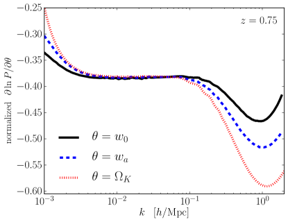
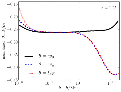
Figure 1 plots the Fisher derivatives for several parameters as a function of $k$, normalized to $k=0.05\,h$/Mpc to highlight the shapes. We see that beyond $k\approx 0.1\,h$/Mpc the curves for the late time parameters such as the dark energy equation of state and curvature begin to diverge, lowering their covariance with each other. Interestingly, at redshifts $z\approx 1.2$–1.6 substantial covariance extends to higher $k$ for $w_{a}$ and $\Omega_{K}$, suggesting that high-redshift galaxy clustering surveys would benefit from combination with lower redshift surveys, or that a survey should span both low and high redshift for best results.

Figure 1: The derivatives $\partial\ln P(k)/\partial\theta$ are plotted vs $k$ for $\theta=\{w_{0},w_{a},\Omega_{K}\}$, at $z=0.75$ (top) and $z=1.25$ (bottom). For clearer comparison of shapes, the $w_{a}$ and $\Omega_{K}$ curves are normalized to the value of the $w_{0}$ curve at $k=0.05\,h$/Mpc.

The final parameter constraints are convolutions of all the Fisher derivatives and their interplay. To illustrate the role of higher $k$ modes in breaking covariances, we plot the absolute value of the correlation matrix, $|r_{ij}|=|C_{ij}|/\sqrt{C_{ii}C_{jj}}$, where $C=F^{-1}$ is the parameter covariance matrix. We focus on the high correlation coefficients (note diagonal entries are 1 by definition). Figure 2 shows these for various $k_{\rm max}$. For clarity the matrix is divided into blocks, with the lower left containing the cosmological parameters, the next (small) block the fiducial bias parameters $\{b^{0}_{\rm ELG},b^{0}_{\rm LRG}\}$, and the upper right block the BNB parameters $\{B_{k},c_{1,k},c_{2,k}\}$. The offdiagonal blocks contain the cross terms.

Figure 2: The absolute value of the correlation coefficients are shown for $k_{\rm max}=0.1$, 0.2 (top row), 0.3, 0.5 (middle), 0.75, $1\,h$/Mpc (bottom row). White space indicates that the correlation coefficient $|r_{ij}|<0.5$. The blocks of cosmology, bias, and baryonic/nonlinear/scale dependent bias (BNB) parameters are labeled. Dotted lines indicate the limit of the $k$ bins from the previous panel in the series.

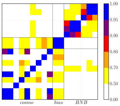
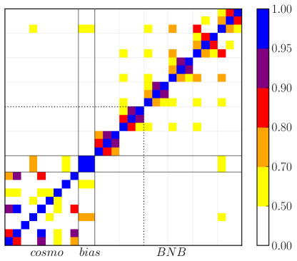
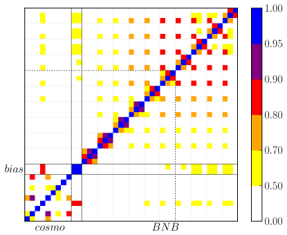
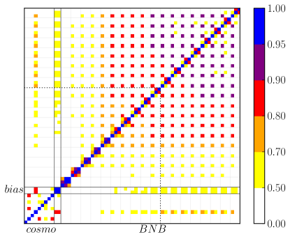
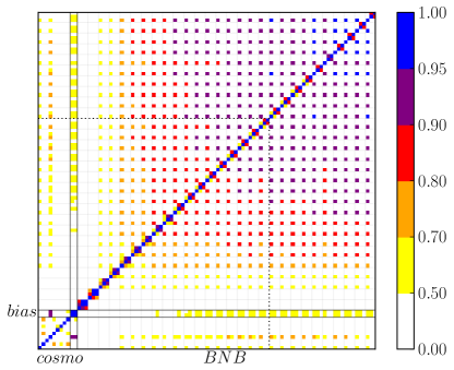
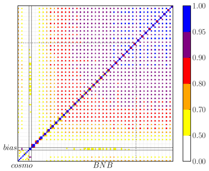
Note that the cosmology parameters become progressively less correlated with each panel at higher $k_{\rm max}$, with the cosmology block becoming both sparser and lighter colored. The BNB parameters, however, retain their correlation (the dotted lines show the size of the matrix from the previous $k_{\rm max}$ step, making it clearer to compare the $k$ bins). Thus, going to higher $k_{\rm max}$ delivers two significant effects in favor of improving cosmology constraints – mode statistics and degeneracy breaking – while the model independent binning approach removes the worry of misestimating the nonlinear or baryonic behavior.

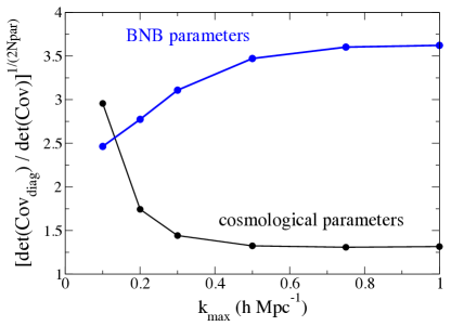
A more compact illustration of the reduction in covariance among cosmological parameters with increasing $k_{\rm max}$ appears in Fig. 3. Here we consider the volumes of the parameter-space ellipsoids in two subspaces: the 9-parameter cosmology space, and the BNB parameter space. In each case, we compare how much the volume (square root of the determinant of the covariance matrix) increases in the hypothetical case that the parameters are completely uncorrelated, versus the actual correlated case. This is a generalized measure of how much correlation there is in the subspace. Because this ratio strongly increases with increasing dimensionality of the subspace, $N_{\rm subspace}$, we also take the $N_{\rm subspace}$-th root of the ratio, making it a “one-parameter equivalent” increase in volume. The ratio is therefore defined as

$$R_{\rm corr}\equiv\left(\frac{\det\,({\rm diag}\,C_{\rm subspace})}{\det\,(C_{\rm subspace})}\right)^{1/(2N_{\rm subspace})}.$$ (10)

When $R_{\rm corr}$ is near unity, the parameter subspace is substantially decorrelated; when it is much larger than unity then covariances play an important role. We see from Fig. 3 that indeed the cosmological parameters become increasingly uncorrelated as $k_{\rm max}$ increases, potentially allowing rapid improvement in their constraints.

Figure 3: The decreasing correlation among cosmological parameters as information is included from beyond the linear regime, to higher $k_{\rm max}$, is demonstrated by taking the volume of their $N$-dimensional ellipsoid including covariances relative to the volume defined by only the product of their variances (see Eq. 10). Baryonic/nonlinear/scale dependent bias parameters, however, are significantly correlated.

Finally, we must assess whether the numerous extra fit parameters for the power spectrum at high $k$ degrade the cosmology estimation. By looking at the cross terms in the cosmo-BNB bands, we see that there is little covariance (the main, though mild, correlation is with $\Omega_{K}$). Thus we expect that the cosmology estimation precision should improve significantly by using these higher $k$ modes, within this marginalized bin approach.

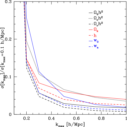
Figure 4 demonstrates this result. The cosmology parameter estimation improves dramatically when going beyond the linear regime, despite the addition of 30, 54, and 114 extra parameters for $k_{\rm max}=0.3$, 0.5, $1\,h$/Mpc. As expected, due to the lingering covariances, $\Omega_{K}$ is the parameter that improves most slowly at higher $k$, while the clear scale dependence of neutrino mass means that it improves most rapidly. Table 2 summarizes the results (again, this should be interpreted predominantly in terms of information content, not actual constraints since the real space power spectrum is not truly an observable quantity in a survey).

Figure 4: The ratio of the parameter uncertainty when using information out to $k_{\rm max}$, relative to using $k_{\rm max}=0.1\,h$/Mpc (so all curves go to 1 at $k_{\rm max}=0.1\,h$/Mpc), is plotted vs $k_{\rm max}$ for several cosmology parameters. The constraints rapidly improve, despite the extra parameters in each $k$ bin for the baryonic/nonlinear/scale dependent bias effects.

$k_{\rm max}$	$10^{3}\Omega_{b}h^{2}$	$10^{3}\Omega_{\rm CDM}h^{2}$	$10^{4}\Omega_{\nu}h^{2}$	$\Omega_{K}$	$100\,h$	$w_{0}$	$w_{a}$	$10^{9}A_{s}$	$n_{s}$	$b^{0}_{\rm ELG}$	$b^{0}_{\rm LRG}$
0.1	4.0	16.0	4.2	0.21	4.8	0.23	1.14	0.53	0.063	0.17	0.33
0.2	0.55	3.2	0.53	0.030	0.70	0.059	0.16	0.082	0.019	0.023	0.045
0.3	0.23	1.8	0.20	0.017	0.33	0.026	0.065	0.037	0.013	0.013	0.026
0.5	0.12	1.1	0.079	0.013	0.19	0.011	0.028	0.016	0.0097	0.0094	0.020
0.75	0.082	0.74	0.043	0.0098	0.14	0.0060	0.017	0.0095	0.0075	0.0075	0.016
1.0	0.070	0.58	0.031	0.0082	0.12	0.0044	0.013	0.0071	0.0063	0.0063	0.013

Table 2: The $1\sigma$ cosmology and fiducial bias parameter uncertainties are given for the baseline survey using information out to various $k_{\rm max}$.

Besides the cosmological parameters, the galaxy linear bias parameters become well determined for $k_{\rm max}\gtrsim 0.2\,h$/Mpc, reaching the $\sim 1\%$ level. Interestingly, the $k$-bin parameters – representing the effects of baryons, nonlinearity, and (scale dependent) galaxy bias on the galaxy power spectrum, not already captured by the Halofit and linear bias models – self calibrate to a large degree. The fractional uncertainties on the bin amplitudes $B_{k}$ tend to be 0.8–1.6%, while the redshift-dependence parameters $c_{1,k}$ and $c_{2,k}$ are determined to about 0.01–0.02, for $k_{\rm max}\gtrsim 0.2\,h$/Mpc.

V Testing Alternatives

The approach of fitting for binned deviations from the Halofit power spectrum gives successful results. Arbitrary deviations, however, could mock up a change in any cosmological parameter, so we should test that the constraints we imposed – on the redshift dependence of the nonlinear deviations and assuming small deviations from Halofit (so the Fisher analysis is in its region of validity) – yield reasonably generic results.

We therefore investigate the effect of altering our baseline approach in three different ways: loosening the redshift dependence, adopting a different fiducial scale dependence, and allowing a mixing between the scale and redshift dependence.

V.1 Redshift dependence

Although a second order polynomial in redshift seems a reasonable treatment for the influence of BNB effects on the power spectrum at $z<2$, we here test its influence by extending the freedom further with a cubic term. That is, Eq. (4) now becomes

$$M(k,z)=(1+c_{1,k}z+c_{2,k}z^{2}+c_{3,k}z^{3})\,B_{k}\ .$$ (11)

This adds one parameter per $k$ bin, giving a total of 83 fit parameters for $k_{\rm max}=0.5\,h$/Mpc say. The fiducial remains $B_{k}=1$, $c_{i,k}=0$.

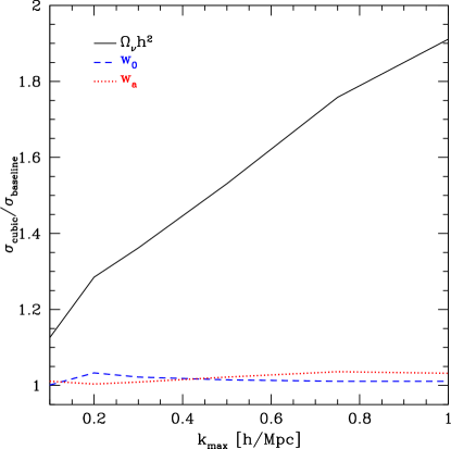
We find that most of the cosmology results are affected little, with less than 10% change in the parameter estimation uncertainties. The main exception is the neutrino energy density constraint, as seen in Fig. 5. Since the neutrino free streaming scale is dependent on both scale and redshift, the extra redshift dependence in the scale dependent BNB factor allows greater covariance, weakening the constraint by less than a factor of 2. The BNB parameters themselves are also less well determined, by factors of up to 1.7 for $B_{k}$ (so uncertainties of 1.3–2%); uncertainties on the three $c_{i,k}$ become up to $\sim$0.07, 0.09, 0.03.

Figure 5: The ratio of the parameter uncertainty when allowing for an extra, cubic redshift fit parameter $c_{3,k}$ in the scale dependence, relative to our baseline fiducial, is plotted vs $k_{\rm max}$ for several cosmology parameters. Only the neutrino energy density shows a significant effect.

V.2 Scale dependence

To treat the BNB effects in as model independent a manner as possible, we allowed free floating bins in $k$ to describe deviations from the (dark matter plus neutrino plus linear bias) Halofit prescription. Since Fisher analysis is only accurate for small deviations around the fiducial, then we may not have accurately captured the effect of large baryonic deviations. Therefore we now adopt a fiducial power spectrum that attempts to include the baryonic effects to high $k$ using the recent work of Mohammed and Seljak (2014). This adds corrections as a polynomial in $k$, whose form is motivated by the Taylor expansion of the 1-halo term in wavenumber $k$. Specifically, rather than take a fiducial of $B_{k}=1$ in each bin, we here use

$$B_{k}=1+(1.33+5.96\,k^{2}-4.63\,k^{4})\,G(k)\ ,$$ (12)

based on the simulation results of Mohammed and Seljak (2014), where in this formula $k$ is in dimensions of $h$/Mpc, $G(k)=F(k)/P_{\rm no\,bary}(k)$, and $F(k)$ is given by their Eq. (30).

We find that this change in fiducial has minimal effect on our results. The maximum fractional change in a parameter uncertainty is 2.7%, with most alterations below 1%. Thus, our results appear robust to this modification.

V.3 Mixing redshift and scale dependence

Some physical effects on the power spectrum may not be well treated by multiplicative factors of scale dependence times redshift dependence (e.g. redshift dependent physical scales such as from baryonic feedback or neutrino free streaming). While our BNB approach does allow mixing of scale and redshift dependence, the fiducial values $c_{i,k}=0$ mean this only enters through the Fisher derivatives, because the fiducial $M_{\rm fid}(k,z)$ in Eq. (4) then becomes independent of $z$. As a simplistic exploration of the possible impact of such an effect, we adopt a fiducial model that makes the redshift dependence vary with scale. Specifically,

$$c_{i,k}=c_{i,\infty}\,\left(1-e^{-k/k_{\star}}\right)\ ,$$ (13)

and rather than the baseline fiducial $c_{i,k}=0$ we set $c_{1,\infty}=2$, $c_{2,\infty}=1$, $k_{\star}=0.3\,h$/Mpc. Thus the fiducial redshift dependence of the BNB effects on the power spectrum stays at the baseline at low $k$, but transitions to $(1+z)^{2}$ at high $k$. This is intended purely as a toy model, with the characteristic that the fiducial deviations are stronger at higher redshift, to test the baseline Fisher analysis.

We find that this mixed fiducial increases correlations among the BNB parameters but has no deleterious effect on estimation of cosmological parameters. Indeed, since for $k\gtrsim k_{\star}$ the fiducial power spectrum is boosted by a factor $(1+z)^{2}$, this enhances $nP_{\rm fid}$ at high $k$ and reduces shot noise, improving most cosmology parameter estimates by $\sim 25\%$.

VI Conclusions

Large scale structure surveys provide a rich array of information on cosmology and astrophysics on scales from the survey size down to small scales, or high wavenumbers. Using this data beyond the linear regime, where we do not fully comprehend all the important physics, is a challenge but one with rich rewards for cosmological understanding. Here we have analyzed how uncertainties in the theoretical prediction for the galaxy power spectrum out to a maximum wavenumber $k_{\rm max}$ impact cosmological parameter constraints, and how we can mitigate the uncertainties without biasing the results.

We included three physical effects: baryonic modifications, nonlinearities, and scale-dependent bias – referred to jointly as the BNB effects. To guard against bias from improperly assuming specific functional forms, we employed a very flexible, nearly model-independent description of the BNB effects that allows scale- and redshift-dependence, described by between 6 and 114 additional fit parameters, depending on $k_{\rm max}$.

Despite the addition of these BNB parameters we could still obtain excellent constraints on cosmology. In fact, the cosmological constraints improve rapidly with increasing $k_{\rm max}$, despite the growing number of extra astrophysical parameters to marginalize over. We traced this improvement to two mutually reinforcing effects: a well-known fact that the information content increases sharply with $k_{\rm max}$ due to more modes, but also the key property that the cosmological parameter correlations weaken as smaller-scale information provides leverage to break degeneracies. We tested this conclusion against different assumptions for the form of the BNB sector, altering the fiducial redshift-, scale-, and mixing of redshift-scale dependence, and found it to be quite robust.

These results agrees qualitatively with other, previous work which shows that cosmological data, and particularly the two-point correlation function, can be remarkably robust with respect to self-calibrating nuisance parameters. In other words, one can add a number of judiciously chosen nuisance parameters that describe the systematic uncertainties, and these parameters, together with cosmological ones, can be internally determined from the data. For example, Wu and Huterer (2013) showed that the three-dimensional galaxy clustering can be used to self-calibrate the parameters describing how galaxies occupy halos (the Halo Occupation Distribution), leading to improvements on small scales despite the rather aggressive modeling of the systematics.

Measuring a large number of nuisance parameters will likely not be feasible due to practical considerations – even if one were able to constrain of order 100 nuisance parameters, doing so might not be robust or convenient in the presence of purely observational and instrument-related systematics which require special care and computational resources in their own right. Fortunately, simpler approaches may bear fruit in the near future. For example, a careful investigation of the effects of baryonic systematics based on a suite of numerical simulations seems to indicate that the systematics span a subspace in the observable (say, the weak lensing angular power spectrum) that is rather orthogonal to that spanned by the cosmological parameters Eifler et al. (2014). Therefore, provided one has successfully modeled the systematics, one can reasonably expect to self-calibrate them or marginalize over their parameters and still be able to constrain the cosmology with excellent accuracy. Again a key issue is guarding against biased results by enhancing both the model independence and the flexibility of the treatment of the BNB effects.

The information content of cosmological data well beyond the linear scale is high. This provides strong motivation to push to large $k_{\rm max}$ while dealing robustly with the baryonic/nonlinearity/scale dependent bias effects masking this signal. The substantially model independent, marginalization approach we present could be a harbinger of rich rewards in cosmological knowledge, without problematic biasing of results, from robust analysis of next generation large-scale-structure measurements.

Appendix A Binning robustness test

The approach taken to treat the BNB uncertainty in the power spectrum is to allow model independent, free floating bin parameters in $k$, with redshift dependence given by a second order polynomial with free coefficients. In Sec. V.1 we tested the impact of allowing further redshift dependence. We would now also like to test the influence of the binning. We chose our fiducial value of $\Delta k=0.025\,h$/Mpc to avoid interaction with the baryon acoustic harmonic of $k\approx 0.06\,h$/Mpc. Here we examine the effect on the cosmological parameter estimation by using $\Delta k=0.01\,h$/Mpc. For $k_{\rm max}=0.5\,h$/Mpc this implies 146 total fit parameters.

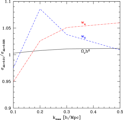
We find that the cosmological parameter uncertainty estimation remains quite robust. The greatest change is an increase in the $n_{s}$ uncertainty by 50% at $k_{\rm max}=0.3\,h$/Mpc (addition of CMB data would constrain $n_{s}$, decreasing the dependence of its estimation on $k_{\rm max}$). For the BNB parameters, constraints weaken due to increased covariance. However our main goals are the estimation of dark energy and neutrino parameters. Figure 6 shows that these uncertainties change by less than 10% with the change in binning, so the results we have presented appear robust.

Figure 6: The ratio of the parameter uncertainty when allowing for a finer binning, $\Delta k=0.01\,h$/Mpc, relative to our baseline fiducial $\Delta k=0.025\,h$/Mpc, is plotted vs $k_{\rm max}$ for several cosmology parameters. The cosmology estimation remains robust.

References

- White (2004) M. J. White, Astropart.Phys. 22, 211 (2004), arXiv:astro-ph/0405593 [astro-ph] .
- Zhan and Knox (2004) H. Zhan and L. Knox, Astrophys.J. 616, L75 (2004), arXiv:astro-ph/0409198 [astro-ph] .
- Huterer and Takada (2005) D. Huterer and M. Takada, Astropart.Phys. 23, 369 (2005), arXiv:astro-ph/0412142 [astro-ph] .
- Huterer and White (2005) D. Huterer and M. J. White, Phys.Rev. D72, 043002 (2005), arXiv:astro-ph/0501451 [astro-ph] .
- Hagan et al. (2005) B. Hagan, C.-P. Ma, and A. V. Kravtsov, Astrophys.J. 633, 537 (2005), arXiv:astro-ph/0504557 [astro-ph] .
- Jing et al. (2006) Y. Jing, P. Zhang, W. Lin, L. Gao, and V. Springel, Astrophys.J. 640, L119 (2006), arXiv:astro-ph/0512426 [astro-ph] .
- Rudd et al. (2008) D. H. Rudd, A. R. Zentner, and A. V. Kravtsov, Astrophys.J. 672, 19 (2008), arXiv:astro-ph/0703741 [ASTRO-PH] .
- Zentner et al. (2008) A. R. Zentner, D. H. Rudd, and W. Hu, Phys.Rev. D77, 043507 (2008), arXiv:0709.4029 [astro-ph] .
- Hearin et al. (2012) A. P. Hearin, A. R. Zentner, and Z. Ma, JCAP 1204, 034 (2012), arXiv:1111.0052 [astro-ph.CO] .
- Zentner et al. (2013) A. R. Zentner, E. Semboloni, S. Dodelson, T. Eifler, E. Krause, et al., Phys.Rev. D87, 043509 (2013), arXiv:1212.1177 [astro-ph.CO] .
- Natarajan et al. (2014) A. Natarajan, A. R. Zentner, N. Battaglia, and H. Trac, Phys. Rev. D 90, 063516 (2014), arXiv:1405.6205 .
- Eifler et al. (2014) T. Eifler, E. Krause, S. Dodelson, A. Zentner, A. Hearin, and N. Gnedin, ArXiv e-prints (2014), arXiv:1405.7423 .
- Harnois-Déraps et al. (2014) J. Harnois-Déraps, L. van Waerbeke, M. Viola, and C. Heymans, ArXiv e-prints (2014), arXiv:1407.4301 .
- Mohammed et al. (2014) I. Mohammed, D. Martizzi, R. Teyssier, and A. Amara, ArXiv e-prints (2014), arXiv:1410.6826 .
- Lewis et al. (2000) A. Lewis, A. Challinor, and A. Lasenby, Astrophys.J. 538, 473 (2000), arXiv:astro-ph/9911177 [astro-ph] .
- Blas et al. (2011) D. Blas, J. Lesgourgues, and T. Tram, JCAP 1107, 034 (2011), arXiv:1104.2933 [astro-ph.CO] .
- Lawrence et al. (2010) E. Lawrence, K. Heitmann, M. White, D. Higdon, C. Wagner, et al., Astrophys.J. 713, 1322 (2010), arXiv:0912.4490 [astro-ph.CO] .
- Heitmann et al. (2014) K. Heitmann, E. Lawrence, J. Kwan, S. Habib, and D. Higdon, Astrophys. J. 780, 111 (2014), arXiv:1304.7849 [astro-ph.CO] .
- Smith et al. (2003) R. Smith et al. (Virgo Consortium), Mon.Not.Roy.Astron.Soc. 341, 1311 (2003), arXiv:astro-ph/0207664 [astro-ph] .
- Senatore and Zaldarriaga (2014) L. Senatore and M. Zaldarriaga, (2014), arXiv:1404.5954 [astro-ph.CO] .
- Mohammed and Seljak (2014) I. Mohammed and U. Seljak, (2014), arXiv:1407.0060 [astro-ph.CO] .
- Takahashi et al. (2012) R. Takahashi, M. Sato, T. Nishimichi, A. Taruya, and M. Oguri, Astrophys.J. 761, 152 (2012), arXiv:1208.2701 [astro-ph.CO] .
- Bird et al. (2012) S. Bird, M. Viel, and M. G. Haehnelt, Mon.Not.Roy.Astron.Soc. 420, 2551 (2012), arXiv:1109.4416 [astro-ph.CO] .
- Linder and Samsing (2013) E. V. Linder and J. Samsing, JCAP 1302, 025 (2013), arXiv:1211.2274 [astro-ph.CO] .
- Feldman et al. (1994) H. A. Feldman, N. Kaiser, and J. A. Peacock, Astrophys.J. 426, 23 (1994), arXiv:astro-ph/9304022 [astro-ph] .
- Seo and Eisenstein (2003) H.-J. Seo and D. J. Eisenstein, Astrophys.J. 598, 720 (2003), arXiv:astro-ph/0307460 [astro-ph] .
- Stril et al. (2010) A. Stril, R. N. Cahn, and E. V. Linder, Mon.Not.Roy.Astron.Soc. 404, 239 (2010), arXiv:0910.1833 [astro-ph.CO] .
- Tegmark et al. (1997) M. Tegmark, A. Taylor, and A. Heavens, Astrophys.J. 480, 22 (1997), arXiv:astro-ph/9603021 [astro-ph] .
- Levi et al. (2013) M. Levi et al. (DESI collaboration), (2013), arXiv:1308.0847 [astro-ph.CO] .
- Laureijs et al. (2011) R. Laureijs et al. (EUCLID Collaboration), (2011), arXiv:1110.3193 [astro-ph.CO] .
- Wu and Huterer (2013) H.-Y. Wu and D. Huterer, Mon.Not.Roy.Astron.Soc. 434, 2556 (2013), arXiv:1303.0835 [astro-ph.CO] .