Minimal Realization Problems for Hidden Markov Models

Abstract

This paper addresses two fundamental problems in the context of Hidden Markov Models (HMMs). The first problem is concerned with the characterization and computation of a minimal order HMM that realizes the exact joint densities of an output process based on only finite strings of such densities (known as HMM partial realization problem). The second problem is concerned with learning a HMM from finite output observations of a stochastic process. We review and connect two fields of studies: realization theory of HMMs, and the recent development in spectral methods for learning latent variable models. Our main results in this paper focus on generic situations, namely, statements that will be true for almost all HMMs, excluding a measure zero set in the parameter space. In the main theorem, we show that both the minimal quasi-HMM realization and the minimal HMM realization can be efficiently computed based on the joint probabilities of length $N$ strings, for $N$ in the order of $\mathcal{O}(\log_{d}(k))$. In other words, learning a quasi-HMM and an HMM have comparable complexity for almost all HMMs.

I Introduction

I-A Background

Hidden Markov Models (HMMs) are widely used for describing discrete random processes, especially in the applications involving temporal pattern recognition such as speech and gesture recognition, part-of-speech tagging and parsing, and bioinformatics. The Markovian property of the hidden state evolution potentially leads to a low complexity representation of the output random process. In this work, we consider the long-standing HMM realization problem: given some partial knowledge about the output process of an unknown HMM, can we generalize it to a full description of the random process?

Consider a discrete random process $\{y_{t}:t\in\mathbb{Z}\}$, which assumes values in a finite alphabet $[d]\equiv\{1,\cdots,d\}$. Assume that $y_{t}$ is the output process of a stationary HMM of finite order. Let the random vector $\mathbf{y}_{1}^{N}=(y_{1},\dots,y_{N})$ denote an string of length $N$, which assumes values in the $N$-ary Cartesian product $[d]^{N}$. The process $y_{t}$ is fully characterized by the joint probabilities of strings of any length in the countably infinite table (denoted by $\mathcal{P}^{(\infty)}$):

$$\Big{\{}\mathbb{P}(y_{1}=l_{1},\cdots,y_{N}=l_{N}):\forall\mathbf{l}_{1}^{N}\in[d]^{N},\forall N\in\mathbb{Z}\Big{\}}.$$

There are three main concerns in the realization problem:

1. (Informational complexity) Suppose that the underlying HMM is of order $k$, and we are given the joint probabilities of all the length $N$ strings, namely:

   $$\mathcal{P}^{(N)}\equiv\Big{\{}\mathbb{P}(y_{1}=l_{1},\cdots,y_{N}=l_{N}):\forall\mathbf{l}_{1}^{N}\in[d]^{N}\Big{\}},$$

   how large does $N$ need to be so that we can compute $\mathcal{P}^{(\infty)}$ based on $\mathcal{P}^{(N)}$?

2. (Computational complexity) Can we solve the realization problem with runtime polynomial in the dimensions (alphabet size $d$ and order of the underlying HMM $k$)?

3. (Statistical complexity) When $\mathcal{P}^{(N)}$ is estimated from sample sequences and has some estimation error, are the realization algorithms robust to the input errors?

These are long standing questions, and there are several lines of work within different communities at tempting to address these questions. It has long been known that, in the information theoretic sense, there exist hard cases of HMMs that are not efficiently PAC learnable [13] [17]. However, a more practical question is, can we efficiently solve the realization / learning problem for most HMMs? In this work, we focus on generic analysis and show that, for almost all HMMs, i.e., excluding those whose parameters are in a measure zero set , the realization problems can be efficiently solved with poly time algorithms.

I-B Organization

To study the HMM realization problems, we focus on algorithms based on the spectral method. The basic idea is to exploit the recursive structural properties of the underlying finite state model, and write the joint probabilities in $\mathcal{P}^{(N)}$ into a specific form which admits rank decomposition, where the rank reveals the minimal order of the realization and the model parameters can be extracted from the factors.

In the first part (Section III), we consider the problem of finding the minimal quasi-HMM realization. Quasi-HMMs are associated with different names in different communities, for example finite state regular automata [4, 5], regular quasi realization [21, 17], and operator models [17, 10]. We mostly follow the terminologies in [21]. Algorithm 1 is the well-known algorithm for finding the minimal order quasi-HMM realization (to be rigorously defined later). However, in general the window size $N$ can not be specified a priori and thus the complexity of the algorithm cannot be explicitly determined. In Theorem 1, we show that, if the output process is generated by an general position HMM with order $k$, we only need the window size $N$ in the order of $\mathcal{O}(\log_{d}(k))$ for pinning down $\mathcal{P}^{(\infty)}$ based on $\mathcal{P}^{(N)}$, where $d$ is the output alphabet size. Moreover, we show that Algorithm 1 has runtime and sample complexity both polynomial in the relevant parameters.

In the second part (Section IV), we consider the problem of finding the minimal HMM realization, using tensor decomposition methods, which rely on the uniqueness of tensor decomposition to recover the minimal order HMM that is unique up to hidden states permutation. Tensor decomposition based algorithms for learning HMMs are studied in [2, 1, 6]. In these works, the transition matrix is always assumed to be of full rank. Similar to that in the quasi-HMM realization problem, in general the required window size $N$ and also the complexity of the algorithm cannot be determined a priori. In [1], the authors examined the generic identifiability conditions of HMM, and showed that generically it suffices to pick the window size $N=2n+1$ for some positive integer $n$, such that ${n+d-1\choose d-1}\geq k$. In the case where $d$ is much smaller than $k$, $n$ needs to be in the order of $\mathcal{O}(k^{1/d})$. Another bound on the window size $N$ is given in [6], which is in the order of $\mathcal{O}(k/d)$. However, the size of the tensor in the decomposition is exponential in $n$, thus all these bound lead to runtime exponential in $k$.

In Section IV, we propose a two-step realization approach, and analyze the identifiability issue of the two steps. Then, we show that for the processes generated by almost all HMMs, the window size $N$ only needs to be in the order of $\mathcal{O}(\log_{d}(k))$ for finding the minimal HMM realization. This means that for most HMMs, finding minimal quasi-HMM and minimal HMM realizations are actually of equal difficulty.

II Minimal realization problem formulation

In this section. we first review the basics of HMMs, and then formally introduce the quasi-HMM and HMM realization problems.

II-A Preliminaries on HMMs

An HMM determines the joint probability distribution over sequences of hidden states $\{x_{t}:t\in\mathbb{Z}\}$ and observations $\{y_{t}:t\in\mathbb{Z}\}$. For simplicity, we call each output $y_{t}$ as a “letter” taking value from some discrete alphabet $[d]$, and a sequence of $n$ letters is referred to as a “string”, taking value from the Cartesian product $[d]^{n}$. We use $[d^{N}]\equiv\{1,\dots,d^{N}\}$ to denote the vectorized indices in $[d]^{n}$.

The joint distribution of $\{x_{t},y_{t}:t\in\mathbb{Z}\}$ from a stationary HMM is parameterized by a pair of matrices: the state transition matrix $Q\in\mathbb{R}_{+}^{k\times k}$, and the observation matrix $O\in\mathbb{R}_{+}^{d\times k}$, which satisfy $\mathbf{e}^{\top}O=\mathbf{e}^{\top}$ and $\mathbf{e}^{\top}Q=\mathbf{e}^{\top}$, where $\mathbf{e}$ is the all ones vector. The hidden state $x_{t}$ evolves following a Markov process:

$$\mathbb{P}(x_{t+1}=j|x_{t}=i)=Q_{j,i}.$$

Let $\pi$ denote the stationary state distribution, i.e., $\pi_{i}=\mathbb{P}[x_{t}=i]$ and $Q\pi=\pi$. Without loss of generality, we assume that $\pi_{i}>0$ for all $i\in[k]$. We also define the backward transition matrix $\widetilde{Q}\in\mathbb{R}^{k\times k}$:

$$\mathbb{P}(x_{t-1}=j|x_{t}=i)=\widetilde{Q}_{j,i}.$$

Observe that the matrix $\widetilde{Q}$ is related to $Q$ as: $\widetilde{Q}=Diag(\pi)Q^{\top}Diag(\pi)^{-1}$. Conditioned on the hidden state taking value $i$, the probability of observing letter $j$ is:

$$\mathbb{P}(y_{t}=j|x_{t}=i)=O_{j,i}.$$

We call two HMMs equivalent if the output processes are statistically indistinguishable.

The order of the HMM is defined to be the number of hidden states, denoted by $k$. We will denote the class of all HMMs with output alphabet size $d$ and order $k$ by $\Theta_{(d,k)}^{h}$.

II-B Problem formulations

The realization problem takes as inputs the probabilities of finite length strings for a fixed window size $N$ ($\mathcal{P}^{(N)}$), and finds a finite state model of the minimal order to describe the entire output process ($\mathcal{P}^{(\infty)}$). We aim to find the most succinct description of the process, namely the minimal order realization, where the “order” refers to the number of states of the underlying finite state model. Without loss of generality, we assume that the process has a minimal realization of order $k$ and examine under what conditions the algorithms can recover an equivalent minimal order realization.

Next, we introduce two classes of finite state models, both of which can realize an HMM output process.

Definition 1 (Quasi-HMM realization [21]).

Let $\theta^{o}$ be a tuple: $\theta^{o}=(k,u,v\in\mathbb{R}^{k},A^{(j)}\in\mathbb{R}^{k\times k}:\forall j\in[d]).$ We call $\theta^{o}$ a quasi-HMM realization of order $k$ for a stationary process $\{y_{t}:t\in\mathbb{Z}\}$ if the three conditions hold: ($\forall\mathbf{l}_{1}^{N}\in[d]^{N},\forall N\in\mathbb{Z}$)

$$\mathbb{P}(\mathbf{y}_{1}^{N}=\mathbf{l}_{1}^{N})=u^{\top}A^{(l_{1})}A^{(l_{2})}\cdots A^{(l_{N})}v,$$ (1)

$$u^{\top}(\sum_{j=1}^{d}A^{(j)})=u^{\top},$$ (2)

$$(\sum_{j=1}^{d}A^{(j)})v=v.$$ (3)

Definition 2 (Equivalent quasi-HMM realizations).

Two quasi-HMM realizations $\theta^{o}=(k,u,v,A^{(j)}:j\in[d])$ and $\widetilde{\theta}^{o}=(k,\widetilde{u},\widetilde{v},\widetilde{A}^{(j)}:j\in[d])$ are called equivalent, if there is a full rank matrix $T\in\mathbb{R}^{k\times k}$ such that:

$$\widetilde{u}={\color[rgb]{0,0,0}{T^{\top}u}},\ \widetilde{v}=T^{-1}v,\ \widetilde{A}^{(j)}=T^{-1}{\color[rgb]{0,0,0}{A^{(j)}}}T,\quad\forall j\in[d].$$

Definition 3 (HMM realization).

Let $\theta^{h}$ be a tuple: $\theta^{h}=(k,O\in\mathbb{R}_{+}^{d\times k},Q\in\mathbb{R}_{+}^{k\times k})$. We call $\theta^{h}$ an HMM realization of order $k$ for a stationary random process $\{y_{t}:t\in\mathbb{Z}\}$, if the matrices $Q$ and $O$ are column stochastic, and the output process of the HMM defined by the transition matrix $Q$ and observation matrix $O$ has the same distribution as $y_{t}$.

HMM realizations are in a subset of the model class of quasi-HMM realizations. Given an HMM realization $\theta^{h}=(k,O,Q)$, one can construct the following quasi-HMM realization $\theta^{o}=(k,u,v,A^{(j)}:j\in[d])$:

$$u=\mathbf{e},$$ (4)

$$v=\pi,$$ (5)

$$A^{(j)}=QDiag(O_{[j,:]}),\quad\forall j\in[d].$$ (6)

The minimal (quasi-)HMM realization problem is formally stated below: Assume that the random process is the output of an HMM of order $k$. How large does the window size $N$ need to be, so that given the joint probabilities $\mathcal{P}^{(N)}$ we can efficiently construct a minimal (quasi-)HMM realization for the process?

III Minimal Quasi-HMM Realization

In this section, we address the minimal quasi-HMM realization problem. We first review the widely used algorithm[3, 5]; then we show for HMMs in general position, the window size $N$ only needs to be in the order of $\mathcal{O}(\log_{d}(k))$ to guarantee the correctness of the algorithm; we also give an example of hard case (degenerate) which needs $N$ to be as large as $k$; finally we examine the stability of the algorithm.

III-A Algorithm

For notational convenience, we define the bijective mapping $L:[d]^{n}\to[d^{n}]$ which maps the multi-index $\mathbf{l}_{1}^{N}=(l_{1},\cdots,l_{n})\in[d]^{n}$ to the index $L(\mathbf{l}_{1}^{n})=(l_{1}-1)d^{n-1}+(l_{2}-1)d^{n-2}+\cdots+l_{n}\in[d^{n}].$

Given the length $N$ joint probabilities $\mathcal{P}^{(N)}$, where $N=2n+1$ for some positive number $n$, we form two matrices $H^{(0)},H^{(j)}\in\mathbb{R}^{d^{n}\times d^{n}}$ for all $j\in[d]$ as below:

$$[H^{(0)}]_{L(\mathbf{l}_{1}^{n}),L(\mathbf{l}_{-1}^{-n})} =\mathbb{P}\Big{(}\mathbf{y}_{-1}^{-n}=\mathbf{l}_{-1}^{-n},\ \mathbf{y}_{0}^{n-1}=\mathbf{l}_{1}^{n}\Big{)},$$ (7)

$$[H^{(j)}]_{L(\mathbf{l}_{1}^{n}),L(\mathbf{l}_{-1}^{-n})} =\mathbb{P}\Big{(}\mathbf{y}_{-1}^{-n}=\mathbf{l}_{-1}^{-n},y_{0}=j,\mathbf{y}_{1}^{n}=\mathbf{l}_{1}^{n}\Big{)},$$ (8)

where $\mathbf{l}_{1}^{n}=(l_{1},\dots,l_{n})$ and ${\color[rgb]{0,0,0}{\mathbf{l}_{-1}^{-n}}}=(l_{-1},l_{-2},\dots,l_{-n})\in[d]^{n}$ denotes the length $n$ string corresponding to the future and the past $n$ time slots, respectively. Note that the “future” observations and the “past” observations are independent conditioned on the “current” state, which is the Markovian property that Algorithm 1 relies on.

Algorithm 1 Minimal quasi-HMM realization

0:  $H^{(0)},H^{(j)}\in\mathbb{R}^{d^{n}\times d^{n}}$ for all $j\in[d]$

0:   $\widetilde{\theta}^{o}=(k,\widetilde{u},\widetilde{v},\widetilde{A}^{(j)}:j\in[d])$

1. Compute the SVD of $H^{(0)}$:

   $$H^{(0)}=U_{H}D_{H}V_{H}^{\prime}.$$ (9)

   Set $U=U_{H}D_{H}^{1/2},\quad V=V_{H}D_{H}^{1/2}$.

2. Let $\widetilde{k}$ be the rank of $H^{(0)}$, and let

   $$\widetilde{u}=U^{\prime}\mathbf{e},\quad\widetilde{v}=V^{\prime}\mathbf{e}.$$ (10)

3. Let $U^{\dagger}$ and $V^{\dagger}$ be the pseudo inverse of $U$ and $V$.

   $$\widetilde{A}^{(j)}=U^{\dagger}H^{(j)}(V^{\dagger})^{\prime},\quad\forall j\in[d].$$ (11)

The core idea of Algorithm 1 was discussed in [11], and it has been rediscovered numerous times in the literature in slightly different forms [3, 5]. We summarize the main idea below.

Remark 1 (Minimal order).

Let $\theta^{o}=(k,u,v,A^{(j)}:j\in[d])$ be a minimal quasi-HMM realization of order $k$ for the process considered. Since the joint probabilities can be factorized in terms of the $A^{(j)}$’s as in (1), one can factorize $H^{(0)}$ and $H^{(j)}$’s as below:

$$H^{(0)}=EF^{\top},\quad H^{(j)}=EA^{(j)}F^{\top},$$

where the matrices $E,F\in\mathbb{R}^{d^{n}\times k}$ are functions of $\theta^{o}$. In particular, the $L(\mathbf{l}_{1}^{n})$-th row of $E$ and $F$ are given by:

$$E_{[L(\mathbf{l}_{1}^{n}),:]}=u^{\top}(A^{(l_{n})}\cdots A^{(l_{1})}),$$ (12)

$$F_{[L(\mathbf{l}_{1}^{n}),:]}=v^{\top}(A^{(l_{n})}\cdots A^{(l_{1})})^{\top}.$$ (13)

Note that if both $E$ and $F$ have full column rank $k$, then $H^{(0)}$ has rank $k$, according to Sylvester’s inequality. Any rank factorization leads to an equivalent minimal quasi-HMM realization of order $k$. The minimal order condition, though not explicitly enforced, is reflected in the rank factorization, as any quasi-HMM realization of lower order results in a matrix $H^{(0)}$ of lower rank, which leads to a contradiction.

The correctness of the algorithm crucially relies on matrix $H^{(0)}$ achieving its maximal rank $k$, which equals the order of the minimal realization. A necessary condition for the correctness of the algorithm is stated below.

Lemma 1 (Correctness of Algorithm 1).

Assume the process has a minimal quasi-realization $\theta^{o}$ of order $k$. Algorithm 1 returns a minimal quasi-HMM realization $\widetilde{\theta}^{o}$ that is equivalent to $\theta^{o}$, if the matrices $E$, $F$ defined in (12) and (13) have full column rank $k$.

Increasing the window size $N$ can potentially boost the rank of $H^{(0)}$, in the hope that the $H^{(0)}$ reaches its maximal rank and Algorithm 1 can correctly finds the minimal realization. However, for a given random process, the study of [19] showed that it is undecidable to verify whether it has a finite order quasi-HMM realization. Even under our assumption that the process indeed has an order $k$ minimal quasi-HMM realization, it is still not clear how large the size of matrix $H^{(0)}$ ($d^{n}\times d^{n}$) needs to be so that it achieves the maximal rank $k$. In previous works, it was usually implicitly assumed that $N$ is large enough so that $H^{(0)}$ achieves its maximal rank [5]. Yet without a bound on $n$ or $N$ the computational complexity of the algorithm is ambiguous.

III-B Generic analysis of information complexity

We desire a small window size $N$ while guaranteeing the full column rank of the matrices $E$ and $F$ defined in (12) and (13). The following theorem shows that if the random process is generated by an order $k$ HMM in general position, then we only need window size $N>4\lceil\log_{d}(k)\rceil+1$ to guarantee the correctness of Algorithm 1.

Theorem 1 (Window size $N$ for quasi-HMM).

1. Consider $\Theta_{(d,k)}^{h}$, the class of all HMMs with output alphabet size $d$ and order $k$. There exists a measure zero set $\mathcal{E}\in\Theta_{(d,k)}^{h}$, such that for all the output process generated by HMMs in $\Theta_{(d,k)}^{h}\backslash\mathcal{E}$, Algorithm 1 returns a minimal quasi-HMM realization, if window size $N=2n+1$ for some $n$ such that:

   $$n>8\lceil\log_{d}(k)\rceil.$$ (14)

2. For any pair of $(d,k)$, randomly pick an instance from the class $\Theta_{(d,k)}^{h}$. If for a given window size $N=2n+1$, the matrix $H^{(0)}$ achieves its maximal rank $k$, then for all HMMs in $\Theta_{(d,k)}^{h}$, excluding a measure zero set, $N$ is sufficiently large for the correctness of Algorithm 1.

Since the elements of matrices $E$ and $F$ are polynomials of the parameters $Q$ and $O$, in order to show $E$ has full column rank for $Q$ and $O$ in general position, it suffices to construct an instance of HMM for which the matrix $E$ has full column rank. In particular, we fix the transition matrix $Q$ and randomize the observation matrix $O$ and bound the singular values of $E$ in probability. The detailed proof is provided in Appendix B.

For all $(d,k)$ pairs in the set $\{2\leq d\leq k<3000\}$, we implemented the test in Theorem 1 (2), and found that for all these cases $n=\lceil\log_{d}(k)\rceil$ is sufficient. We conjecture that in general, $n\geq\log_{d}(k)$ is enough.

In the worst case [21], the “Hankel rank” of the matrix $H^{(0)}$ with infinite window size can be larger than the rank of any finite size block of the infinite matrix. Instead of the worst case analysis, our generic analysis examines the average cases, and it has the following implications: if the process is generated by some average case HMM of order $k$, then the Hankel rank equals $k$; moreover, the window size $n$ only needs to be in the order of $O(\log_{d}(k))$ so that the rank of finite matrix $H^{(0)}$ achieves the Hankel rank.

III-C Existence of hard cases

We showed that for generic HMM output processes, Algorithm 1 is has polynomial runtime. There exists a long line of hardness results for learning HMMs [13, 17, 20], showing that in the worst case (lie in the measure zero set in the parameter space) learning the distribution of an HMM can be computationally hard under cryptographic assumptions.

In Fig. 1, we adapt the hardness results to our setting and give an example. The state diagram describes the transition and observation probabilities. Solving the realization problem is equivalent to learning the joint distribution of the process. One can verify that the window size $N$ needs to be at least as large as $T$, which is proportional to the order of the underlying HMM, and therefore the computation complexity is exponential in the order of the HMM.

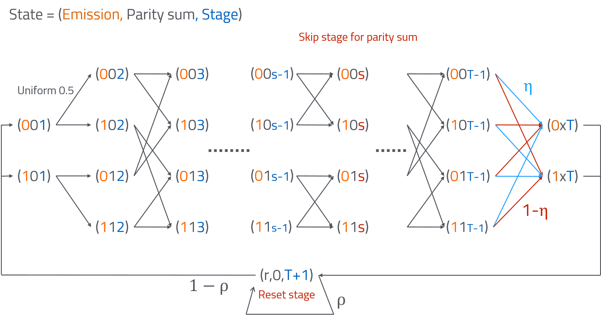
Figure 1: Reduction of HMM to noisy parity to lower bound the worst case computational complexity. In the state transition diagram, for stage $t=1,\cdots,T-1$, the emission state $E_{t}$ is uniformly distributed over $\{0,1\}$ and is observed. For stage $t=2,\cdots,T-1$, the parity state $S_{t}$ computes $E_{t-1}\oplus S_{t-1}$, except for at one unknown stage $s$, $S_{t}=S_{t-1}$. At stage $T$, with probability $\eta$, the correct parity state $S_{T-1}$ is revealed, and with probability $1-\eta$, the complement is observed. $(T+1)$ is a reset stage, with probability $\rho$ it stays in the reset stage.

We point out that not all HMMs in the measure zero set are information theoretically hard to learn. For instance, consider the degenerate HMM in [1] with the transition matrix $Q=I_{k\times k}$ and with general position observation matrix $O$. Suppose that $d\ll k$, it was shown that the window size $N$ needs to be in the order of $k^{1\over d}$ so that matrices $E$ and $F$ attain full column rank. However the distribution of this i.i.d. process is not fundamentally difficult to learn. It remains an open problem to find realization algorithm that can handle more cases.

III-D Stability analysis

In practice, the joint probabilities in $\mathcal{P}^{(N)}$ are estimated based on finite sample sequences of the process. In the next theorem, we show that in order to achieve $\epsilon$-accuracy in the parameters of the minimal quasi-HMM realization, the number of sample sequences we need to estimate $\mathcal{P}^{(N)}$ is polynomial in all relevant parameters, including the order $k$.

Theorem 2.

Given $T$ independent sample sequences of the output process of an HMM of order $k$ and with alphabet size $d$. Construct $\widehat{H}^{(0)}$ and $\widehat{H}^{(j)}$’s as in (7) and (8) with the empirical probabilities. Let $N=2n+1$, and $n=2\lceil\log_{d}(k)\rceil$. Let $\widehat{\theta}^{o}=(k,\widetilde{u},\widetilde{v},\widetilde{A}^{(j)}:j\in[d])$ and $\widetilde{\theta}^{o}=(k,\widetilde{u},\widetilde{v},\widetilde{A}^{(j)}:j\in[d])$ be the output of Algorithm 1 with the empirical probabilities and the exact probabilities for the input, respectively. Then, in order to achieve $\epsilon$-accuracy in the output with probability at least $1-\eta$, namely:

$$\|\widehat{u}-\widetilde{u}\|\leq\epsilon,\ \|\widehat{v}-\widetilde{v}\|\leq\epsilon,\ \|\widehat{A}^{(j)}-\widetilde{A}^{(j)}\|\leq\epsilon,\forall j,$$

the number of independent sample sequences we need is given by:

$$T={Ck^{6}d^{4}\over\epsilon^{4}\sigma_{k}^{8}}\log\left({2k^{4}d^{2}\over\eta}\right),$$

where $\sigma_{k}$ is the $k$-th singular value of $H^{(0)}$ and $C$ is some absolute constant.

Since the core of the algorithm is singular value decomposition of the matrix $H^{(0)}$, the stability analysis mostly uses the standard matrix perturbation results, which we review in Appendix C. The detailed proof is provided in Appendix B.

Remark 2.

Note that Theorem 1 shows that for window size $N$ large enough ($O(\log_{d}(k))$), the exact realization problem (no estimation noise) can be solved with poly time algorithm. When empirical probabilities are used, Theorem 2 shows that the required number of independent samples is polynomial in $k$, $d$, and $1/\sigma_{k}$. $\sigma_{k}$ depends on the HMM that generates the process. In the proof of Theorem 1, it is showed that there exist cases for which $\sigma_{k}$ is lower bounded by constant, for which case the sample complexity is indeed polynomial; however there also exists hard cases for which $\sigma_{k}$ is arbitrarily small. We defer the analysis of sample complexity, which relies on understanding the relation between window size, HMM parameter, and $\sigma_{k}$, to future work.

IV Minimal HMM Realization Problem

Recall that an HMM can be easily converted to a quasi-HMM of the same order as shown in (4)–(6), yet given a quasi-HMM realization it is difficult to construct an HMM [3]. In this section, we apply tensor decomposition techniques to study the minimal HMM realization problem and discuss its connection to the previous section. In particular, we show that for processes generated by general position HMMs, the two realization problems have similar computational complexity.

IV-A Preliminaries on tensor algebra

Definitions

Tensor algebra has many similarities to but also many striking differences from matrix algebra, one of which is that, under very mild conditions, tensor minimal rank decomposition is unique up to column scaling and permutation, which is the key property exploited to uniquely identify the minimal HMM realization. This is in parallel with the fact that we use matrix rank decomposition to find a minimal quasi-HMM realization.

We review some properties of 3rd order tensors below. A more detailed introduction to tensor algebra can be found in [14] and the references therein. One way to view a 3rd order tensor $X\in\mathbb{R}^{n_{A}\times n_{B}\times n_{C}}$ is that it defines a three-way array, multi-indexed by $(j_{1},j_{2},j_{3})$, $\forall j_{1}\in[n_{A}],j_{2}\in[n_{B}],j_{3}\in[n_{C}]$. A rank-1 tensor $X=a\otimes b\otimes c$ is defined to be the outer-product of the three vectors $a,b,c$ and $X_{j_{1},j_{2},j_{3}}=a_{j_{1}}b_{j_{2}}c_{j_{3}}$. Tensor rank decomposition is a natural extension of matrix singular value decomposition (SVD) to higher order tensors.

Definition 4 (Tensor rank decomposition).

The rank decomposition of a 3rd order tensor $X\in\mathbb{R}^{n_{A}\times n_{B}\times n_{C}}$ is a sum of rank-1 tensors for the smallest number of summands $k$:

$$X=A\otimes B\otimes C=\sum_{i=1}^{k}A_{[:,i]}\otimes B_{[:,i]}\otimes C_{[:,i]},$$

where matrices $A\in\mathbb{R}^{n_{A}\times k}$, $B\in\mathbb{R}^{n_{B}\times k}$, $C\in\mathbb{R}^{n_{C}\times k}$. The minimal number of summands $k$ is defined to be the rank of the tensor.

A tensor can also be viewed as a multi-linear operator. Consider a 3rd order tensor $X$. For given $m_{A},m_{B},m_{C}$, it defines a multi-linear mapping $X(V_{1},V_{2},V_{3}):\mathbb{R}^{m_{A}\times n_{A}}\times\mathbb{R}^{m_{B}\times n_{B}}\times\mathbb{R}^{m_{C}\times n_{C}}\to\mathbb{R}^{m_{A}\times m_{B}\times m_{C}}$ as below: $(\forall j_{1}\in[m_{A}],j_{2}\in[m_{B}],j_{3}\in[m_{C}])$

$$[X(V_{1},V_{2},V_{3})]_{j_{1},j_{2},j_{3}}$$ (15)

$$= \sum_{i_{1}\in[n_{A}],i_{2}\in[n_{B}],i_{3}\in[n_{C}]}X_{i_{1},i_{2},i_{3}}[V_{1}]_{j_{1},i_{1}}[V_{2}]_{j_{2},i_{2}}[V_{3}]_{j_{3},i_{3}}.$$

Assuming that the tensor admits a decomposition $X=A\otimes B\otimes C\in\mathbb{R}^{n_{A}\times n_{B}\times n_{C}}$, we can equivalently write:

$$X(V_{1},V_{2},V_{3})=(V_{1}A)\otimes(V_{2}B)\otimes(V_{3}C),$$ (16)

Note that $X$ can have different forms of decompositions, yet the mappings defined in (16) are all equivalent.

Definition 5 (Khatri-Rao product).

For matrices $A\in\mathbb{R}^{n_{A}\times k}$, $B\in\mathbb{R}^{n_{B}\times k}$, the (column) Khatri-Rao product $X=A\odot B\in\mathbb{R}^{n_{A}n_{B}\times k}$ is defined as follows:

$$X_{(j_{1}-1)n_{B}+j_{2},i}=A_{j_{1},i}B_{j_{2},i},$$

and each column of $X$ is a rank-1 Khatri-Rao product.

An equivalent representation of a 3rd order tensor $X\in\mathbb{R}^{n_{A}\times n_{B}\times n_{C}}$ is given by its matricization, obtained by rearranging the elements of the tensor into a matrix. For example, the matricization along the third mode gives a matrix $\overline{X}^{(3)}$ is specified as below:

$$\left[\overline{X}^{(3)}\right]_{j_{3},\ ((j_{1}-1)n_{B}+j_{2})}=X_{j_{1},j_{2},j_{3}}.$$

Moreover, if the tensor admits a decomposition $X=A\otimes B\otimes C$, we can write the matricization as Khatri-Rao product of the factors: $\overline{X}^{(3)}=C(A\odot B)^{\top}$.

Uniqueness condition

Unlike the rank decomposition of matrices, under rather mild conditions of the factors we can uniquely (up to common column permutation and scaling) identify the factors from the 3rd order tensor $X$ In the following, we state a set of sufficient conditions on the factors $A,B,C$ that guarantee the uniqueness of tensor decomposition,

Definition 6 (Kruskal rank).

The Kruskal rank of a matrix $A\in\mathbb{R}^{n\times m}$ equals $r$ if any set of $r$ columns of $A$ are linearly independent, and there exists a set of $(r+1)$ columns that are linearly dependent (if $r<m$).

Lemma 2 (Uniqueness of tensor decomposition ([15, 18])).

The tensor factorization $X=A\otimes B\otimes C$ is unique up to column permutation and scaling, if

$$krank(A)+krank(B)+krank(C)\geq 2k+2.$$ (17)

Decomposition algorithms

Unlike matrix SVD, in general tensor decomposition is a hard problem [14]. Nevertheless, for cases where the factors $A,B,C$ satisfy certain rank conditions, there exist efficient and provable algorithms. We include the detailed steps of the algorithm in the appendix for completeness.

If the matrix $A$ and $B$ both have full column rank, Algorithms 3 in the appendix ([16]) can uniquely recover the factors up to common column permutation, with running time polynomial in the dimension of the tensor. Other algorithms such as tensor power method and recursive projection, which are possibly more stable in practice, also apply here.

Algorithm 4 is another efficient tensor decomposition algorithm ([8] [12]) to a subset of the degenerate instances whose transition matrix is rank deficient. Instead of requiring both $A$ and $B$ to be of full rank $k$, this algorithm requires that the factor $C$ and the Khatri-Rao product $A\odot B$ have full column rank $k$. The basic idea of the algorithm is as follows: there is a unique rank decomposition of the 3rd dimension matricization of the tensor: $\overline{X}^{(3)}=FE^{\top}=C(A\odot B)^{\top}$, under the algebraic constraints that each column of the matrix $E$ is a rank one Katri-Rao product.

IV-B Minimal HMM realization

Formulation

For a fixed window size $N=2n+1$, given the exact joint probabilities in $\mathcal{P}^{(N)}$, similar to the construction of $H^{(0)}$ in (7), one can construct a 3rd order tensor $M\in\mathbb{R}^{d^{n}\times d^{n}\times d}$ as below:

$$M_{\ L(\mathbf{l}_{1}^{n}),L(\mathbf{l}_{-1}^{-n}),\ l_{0}}=\mathbb{P}\Big{(}\mathbf{y}_{-n}^{n}=\mathbf{l}_{-n}^{n}\Big{)},\quad\forall\mathbf{l}_{-n}^{n}\in\mathbb{[}d]^{N}.$$ (18)

Suppose that the process has a minimal HMM realization $\theta^{h}=(k,Q,O)$ of order $k$. We can write $M$ as a tensor product:

$$M=A\otimes B\otimes C,$$ (19)

where the matrices $A,B\in\mathbb{R}^{d^{n}\times k}$ and $C\in\mathbb{R}^{d\times k}$ correspond to the conditional probabilities:

$$A_{L(\mathbf{l}_{1}^{n}),m} =\mathbb{P}\Big{(}\mathbf{y}_{1}^{n}=\mathbf{l}_{1}^{n}\Big{|}x_{0}=m\Big{)},$$ (20)

$$B_{L(\mathbf{l}_{-1}^{-n}),m} =\mathbb{P}\Big{(}\mathbf{y}_{-1}^{-n}=\mathbf{l}_{-1}^{-n}\Big{|}x_{0}=m\Big{)},$$ (21)

$$C_{l,m} =\mathbb{P}\Big{(}y_{0}=l,x_{0}=m\Big{)}.$$ (22)

Moreover, observe that $A$ anh $B$ are recursive linear functions of the model parameters $Q$ and $O$ as below:

$$A^{(n)} =\mathbb{P}\Big{(}\mathbf{y}_{1}^{n}\Big{|}x_{0}=m\Big{)}=(O\odot A^{(n-1)})Q,$$ (23)

$$B^{(n)} =\mathbb{P}\Big{(}\mathbf{y}_{-1}^{-n}\Big{|}x_{0}=m\Big{)}=(O\odot B^{(n-1)})\widetilde{Q},$$ (24)

and $A^{(1)}=OQ$ and $B^{(1)}=O\widetilde{Q}$. In particular, for the given window size $N=2n+1$, we have:

$$A=A^{(n)},\quad B=B^{(n)},\quad C=ODiag(\pi).$$ (25)

The basic idea of recovering the minimal HMM realization $\theta^{h}$ (up to hidden state relabeling) is to first recover the factors $A,B$ and $C$ via tensor decomposition, and then extract the transition and observation probabilities from the factors. The minimal order condition is again reflected in the tensor rank factorization, as any HMM realization of lower order results in a tensor $M$ of lower tensor rank, which is a contradiction.

Identifiability

The identifiability of the minimal HMM relies on the fact that the tensor rank decomposition indeed recovers the factor $A,B,C$ defined in (20)–(22). Note that by definition, the column stochastic observation matrix $O$ must have Kruskal rank greater than $2$, otherwise there exist two identical columns in $O$, and the corresponding two hidden states can be merged to give an equivalent HMM realization of smaller order.

Lemma 3 (Uniqueness of tensor decomposition).

Given window size $N$, if the matrices $A,B\in\mathbb{R}^{d^{n}\times k}$ defined in (23)–(25) have full column rank $k$, then $M$ can be uniquely decomposed into column stochastic matrices $A,B,C$ as in (19) (up to common column permutation).

In parallel with Theorem 1, the next theorem shows that the condition above is satisfied for a general position HMM process with sufficiently large window size $N$.

Theorem 3 (Choice of $N$ for HMM realization).

Consider $\Theta^{h}_{(d,k)}$, the class of all HMMs with output alphabet size $d$ and order $k$. There exists a measure zero set $\mathcal{E}\in\Theta_{(d,k)}^{h}$ such that for all output processes generated by HMMs in the set $\Theta_{(d,k)}^{h}\backslash\mathcal{E}$, the minimal quasi-HMM realization can be computed based on the joint probabilities in $\mathcal{P}^{(N)}$, if window size $N=2n+1$ for some $n$ such that:

$$n>8\lceil\log_{d}(k)\rceil.$$ (26)

Algorithms

The matrices $A,B$ and $C$, defined in (23)–(25), are polynomial functions of the parameters $Q$ and $O$ of the minimal HMM realization. The following theorem exploits the recursive structure of these polynomials to recover the parameters $Q$ and $O$ if the factors $A,B,C$ are given.

Theorem 4 (Recovering $Q$ and $O$ from $A,B,C$).

Given the matrix $C$, one can obtain the observation matrix by:

$$O_{[:,i]}={C_{[:,i]}/(\mathbf{e}^{\top}C_{[:,i]})},\quad\forall i\in[k].$$ (27)

Given the matrix $A\in\mathbb{R}^{d^{n}\times k}$, we first scale each of the column similar to (27) so that each column is stochastic, and corresponds to the conditional probabilities $\mathbb{P}(\mathbf{y}_{1}^{n}|x_{0})$ as shown in (20). We marginalize the conditional distribution to get $A^{(1)}=\mathbb{P}\left(y_{1}|x_{0}\right)\in\mathbb{R}^{d\times k}$ and $A^{(n-1)}=\mathbb{P}\left(\mathbf{y}_{1}^{n-1}\big{|}x_{0}\right)\in\mathbb{R}^{d^{n-1}\times k}$.

1. If $A$ has full column rank $k$ ([1]):

   $$Q=\Big{(}O\odot A^{(n-1)}\Big{)}^{\dagger}A.$$ (28)

2. If $C$ has full column rank $k$:

   $$Q=O^{\dagger}A^{(1)}.$$ (29)

   where $(X)^{\dagger}=(X^{\top}X)^{-1}X^{\top}$ denotes the pseudo-inverse of a matrix $X$.

In the proof of Theorem 3, we show that for general position HMMs with sufficiently large window size, the matrices $A$ and $B$ achieve full column rank $k$. When this holds, Algorithm 3 computes the unique tensor decomposition to recover the factors $A,B,C$. Theorem 4 (1) applies to recover $Q$ and $O$ from the factors.

However, if the transition matrix $Q$ of the minimal HMM realization does not have full rank, and no matter how large the window size is, the matrix $A$ never achieves full rank. Note that these HMMs are degenerate cases belonging to the measure zero set in Theorem 3, and Algorithm 3 is not applicable for decomposing the tensor $M$. However, it is still possible to apply Algorithm 4. Note that a necessary condition for it to work is that $d\geq k$ and the observation matrix is of full column rank.

Let $\Theta_{(d,k,r)}^{h}$ denote the model class of HMMs with output alphabet $d$ and order $k$, for $d\geq k$ and the transition matrix $Q$ has rank $r<k$. Note that $\Theta_{(d,k,r)}^{h}$ is a subset of the measure zero set $\mathcal{E}$ in Theorem 3. The following theorem shows that if Algorithm 4 runs correctly for a random instance in this subset, then the algorithm works for almost all HMMs in this subset.

Theorem 5 (Correctness of Algorithm 4).

Given $d,k$ and $r$ and consider the set $\Theta_{(d,k,r)}^{h}$. Let $A,B,C$ be defined as in (23)– (25) for $n=1$, and let $M=A\otimes B\otimes C$. If Algorithm 2 returns “yes”, then there exists a measure zero set $\mathcal{E}\in\Theta_{(d,k,r)}^{h}$, such that Algorithm 4 returns the tensor decomposition $M=A\otimes B\otimes C$ for all HMMs in the set $\Theta_{(d,k,r)}^{h}\backslash\mathcal{E}$. Moreover, if the latter is true, Algorithm 2 returns “yes” with probability 1.

For this class of degenerate HMMs, Theorem 4 (2) applies to recover $Q$ and $O$.

Note that for both the general position case and this degenerate case, the computation complexity to recover the parameters of the minimal HMM realization are polynomial in both $d$ and $k$, and this is an immediate result of the log upper bound of the window size.

Algorithm 2 Check Condition

1. Randomly choose an HMM from $\theta^{h}\in\Theta_{(d,k,r)}^{h}$.

2. Construct matrices $A,B,C$ with $(Q,O)$ as defined in (23)–(25) for $n=1$, namely $A=OQ$, $B=O\widetilde{Q}$, and $C=ODiag(\pi)$.

3. Let $M=A\otimes B\otimes C$. Run Algorithm 4 with the input $M$.

4. Return “yes” if the algorithm returns $A,B,C$ uniquely up to a common column permutation, and “no” otherwise.

V Conclusion

In this paper, we discussed two realization problems. We show that for output processes generated by HMMs in general position, both learning the minimal quasi-HMM realization and learning the real minimal HMM realization are easy– in the sense that there exist efficient algorithms to compute the minimal realizations with running time and sample complexity both polynomial in the relevant parameters of the problem.

Appendix A Tensor decomposition algorithms

For completeness, we list two standard tensor decomposition algorithms in this section.

Algorithm 3 Simultaneous diagonalization for 3rd order tensor decomposition [16]

0:   A 3rd order tensor $M\in\mathbb{R}^{d^{n}\times d^{n}\times d}$

0:   $k,A,B\in\mathbb{R}^{d^{n}\times k},C\in\mathbb{R}^{d\times k}$

1. Randomly pick two unit norm vectors $\mathbf{v}_{1},\mathbf{v}_{2}\in\mathbb{R}^{d}$. Project $M$ along the 3rd dimension to obtain two matrices:

   $$\widetilde{M}_{1}=M(I,I,\mathbf{v}_{1}),\quad\widetilde{M}_{2}=M(I,I,\mathbf{v}_{2}).$$

2. Compute the eigen-decomposition of matrix $(\widetilde{M}_{1}\widetilde{M}_{2}^{-1})$ and $(\widetilde{M}_{2}\widetilde{M}_{1}^{-1})$, and let the columns of matrix $A$ and $B$ be the eigenvectors of $(\widetilde{M}_{1}\widetilde{M}_{2}^{-1})$ and $(\widetilde{M}_{2}\widetilde{M}_{1}^{-1})$, respectively.

   Scale the columns of $A$ and $B$ to be stochastic, and pair the eigenvectors in $A$ and $B$ corresponding to the reciprocal eigenvalues, namely:

   $$\widetilde{M}_{1}\widetilde{M}_{2}^{-1}=A\Lambda A^{-1},\quad\widetilde{M}_{2}\widetilde{M}_{1}^{-1}=B\Lambda^{-1}B^{-1}.$$

3. Let $k$ be the number of non-zero eigenvalues.

4. Let $\overline{M}^{(3)}\in\mathbb{R}^{d^{2n}\times d}$ be the 3rd dimension matricization of $M$. Set $C$ to be:

   $$C=\overline{M}^{(3)}((A\odot B)^{\dagger})^{\top}$$

Algorithm 4 FOOBI for 3rd order tensor decomposition

0:  $M\in\mathbb{R}^{d\times d\times d}$

0:   $k,A,B,C.$

1. Let $\overline{M}^{(3)}$ be the 3rd dimension matricization of $M$. Compute its SVD $\overline{M}^{(3)}=V_{H}D_{H}U_{H}^{\top}$.

2. Set $k$ to be the number of non-zero singular values. Let $F=V_{H}D_{H}^{1/2}$, and $E=U_{H}D_{H}^{1/2}$.

3. Construct matrices $\{E^{(r)}\in\mathbb{R}^{d\times d}:r\in[k]\}$:

   $$[E^{(r)}]_{i,j}=E_{(i-1)d+j,r},\forall i,j\in[d],\ \forall r\in[k].$$

   Construct the 4-th order tensors $\{P^{(r,s)}\in\mathbb{R}^{d\times d\times d\times d}:r,s\in[k]\}$:

   $$[P^{(r,s)}]_{i_{1},i_{2},j_{1},j_{2}}$$

   $$=[E^{(r)}]_{i_{1},j_{1}}[E^{(s)}]_{i_{2},j_{2}}+[E^{(s)}]_{i_{1},j_{1}}[E^{(r)}]_{i_{2},j_{2}}$$

   $$-[E^{(r)}]_{i_{1},j_{2}}[E^{(s)}]_{i_{2},j_{1}}-[E^{(s)}]_{i_{1},j_{2}}[E^{(r)}]_{i_{2},j_{1}}.$$

4. Compute a basis $\{H^{(i)}:i\in[k]\}$ of the $k$-dimensional kernel of $\{P^{(r,s)}:r,s\in[k]\}$:

   $$\sum_{r,s=1}^{k}H_{r,s}^{(i)}P^{(r,s)}=0,\ \text{ s.t. }H_{r,s}^{(i)}=H_{s,r}^{(i)},\forall r,s\in[k].$$

5. Find the unique $W\in\mathbb{R}^{k\times k}$ that simultaneously diagonalizes the basis:

   $$H^{(i)}=W\Lambda^{(i)}W^{\top},\ \forall i\in[k].$$

6. Let $C=F(W^{-1})^{\top}$ and $A\odot B=EW$. Compute the rank one decomposition of each column of $A\odot B$, with proper normalization such that $A$ and $B$ are column stochastic.

Appendix B Proofs

(Proof of Lemma 1)

If both $E$ and $F$ have full column rank $k$, by Sylvester inequality the rank of the matrix $H^{(0)}$ is also equal to $k$, the order of minimal quasi-HMM realization. Therefore, for the two matrices $U$ and $V$ obtained in Step 2 in Algorithm 3, there exists some full rank matrix $W\in\mathbb{R}^{k\times k}$ such that:

$$U=EW,\quad V^{\top}=W^{-1}F^{\top}.$$

Therefore, Step 3 returns

$$\widetilde{A}^{(j)}=W^{-1}E^{\dagger}EA^{(j)}F^{\top}(F^{\top})^{\dagger}W=W^{-1}A^{(j)}W.$$

By the normalization constraint in Definition 1, we have

$$u^{\top}W=u^{\top}\sum_{j=1}^{d}A^{(j)}W=u^{\top}W\sum_{j=1}^{d}\widetilde{A}^{(j)}.$$

Moreover, since

$$U =\left[\begin{array}[c]{c}u^{\top}(A^{(1)}\cdots A^{(1)})\\ u^{\top}(A^{(1)}\cdots A^{(2)})\\ \vdots\\ u^{\top}(A^{(d)}\cdots A^{(d)})\end{array}\right]W=u^{\top}W\left[\begin{array}[c]{c}\widetilde{A}^{(1)}\cdots\widetilde{A}^{(1)}\\ \widetilde{A}^{(1)}\cdots\widetilde{A}^{(2)}\\ \vdots\\ \widetilde{A}^{(d)}\cdots\widetilde{A}^{(d)}\end{array}\right],$$

in Step 2 we obtain $\widetilde{u}^{\top}=u^{\top}W,$ and similarly, we can argue that $\widetilde{v}=W^{-1}v$. Thus we conclude that the output $\widetilde{\theta}^{o}=(k,\widetilde{u},\widetilde{v},\widetilde{A}^{(j)}:j\in[d])$ is a valid minimal quasi-HMM realization of order $k$, and is equivalent to $\theta^{o}$ up to a linear transformation.

∎

(Proof of Theorem 1)

Assume that the observed process has a minimal HMM realization $\theta^{h}$ of order $k$, i.e., $\theta^{h}\in\Theta^{h}_{(d,k)}$, and let $\theta^{o}$ denote the equivalent order $k$ quasi-HMM as shown in (4)-(6). For window size $N=2n+1$, define the matrices $E$ and $F$ for $\theta^{o}$ as in (12) and (13) and note that:

$$E_{L(\mathbf{l}_{1}^{n}),i}$$

$$=[u^{\top}(A^{(l_{n})}\cdots A^{(l_{1})})]_{i}$$

$$=\mathbf{e}^{\top}\mathbb{P}(x_{n},y_{n-1}=l_{n}|x_{n-1})\cdots\mathbb{P}(x_{1},y_{0}=l_{1}|x_{0}=i)$$

$$=\mathbb{P}\Big{(}\mathbf{y}_{0}^{n-1}=\mathbf{l}_{1}^{n}\Big{|}x_{0}=i\Big{)},$$

and similarly,

$$F_{L(\mathbf{l}_{1}^{n}),i} =[A^{(l_{n})}\cdots A^{(l_{1})}\pi]_{i}=\mathbb{P}\Big{(}\mathbf{y}_{-1}^{-n}=\mathbf{l}_{1}^{n},x_{0}=i\Big{)}.$$

Lemma 1 shows that a sufficient condition for the correctness of Algorithm 1 is that both $E$ and $F$ have full column rank $k$. In this proof, we show that when $Q$ and $O$ of the HMM $\theta^{h}\in\Theta^{h}_{(d,k)}$ are in general position, this rank condition is satisfied if the window size $N=2n+1$ satisfies (14).

Note that the minors of $E$ and $F$ are polynomials in the elements of $Q$ and $O$, thus it defines a algebraic set in the parameter space by setting all the minors to zero to make $E$ and $F$ to be rank deficient. By basic algebraic geometry [9], the algebraic set either occupies the entire Zariski closure or is a low-dimensional manifold of Lebesgue measure zero. In particular, the Zariski closure of $\Theta_{(d,k)}^{h}$, defined to be the smallest algebraic set containing $\Theta_{(d,k)}^{h}$, is given by $\overline{\Theta}_{(d,k)}^{h}:=\{O\in\mathbb{R}^{d\times k},Q\in\mathbb{R}^{k\times k}:\mathbf{e}^{\top}O=\mathbf{e}^{\top},\mathbf{e}^{\top}Q=\mathbf{e}^{\top}\}$ (note that the element-wise non-negativity constraints can be omitted when considering the Zariski closure). Therefore, it is enough to show that for some specific choice of $Q$ and $O$ in $\overline{\Theta}_{(d,k)}^{h}$, the matrices $E$ and $F$ achieve full column rank $k$. Moreover to construct an instance, we can further ignore the stochastic constraints, as scaling does not the independence property of the columns in $E$ and $F$.

We fix the transition matrix $Q$ to be the state shifting matrix as below:

$$Q_{i-1,i}=1,\text{ for }2\leq i\leq k,\text{ and }\quad Q_{k,1}=1,$$ (30)

Note that with this choice of $Q$, $\pi={1\over k}\mathbf{e}$, and $\widetilde{Q}=Q^{\top}$. Due to the symmetry of the forward and backward transitions, we can focus on showing that $E$ has full column rank and the same argument applies to $F$.

We randomize the observation matrix $O$ and let the columns be independent random variables uniformly distributed on the $d$-dimensional sphere. In order to show that there exists a construction of $(Q,O)$ such that $E$ has full column rank, it suffices to show that $E$ achieves full column rank with positive probability over the randomness of $O$. We apply Gershgorin’s theorem to prove that the columns of $E$ are incoherent.

Note that for the shifting matrix $Q$, we have:

$$E_{[:,i]}=O_{[:,i]}\odot\cdots O_{[:,i+n-1]}.$$

Since we have $d\geq 2$ and $n<k$, for notational convenience, we slightly abuse notation to write the $j$-th column of $O$ as $O_{[:,j]}$, while for $k<j\leq 2k$, it actually refer to the $(j-k)$-th column of $O$.

Define matrix $X\in\mathbb{R}^{k\times k}$ to be:

$$X_{i,j}=E_{[:,i]}^{\top}E_{[:,j]}=\prod_{m=0}^{n-1}(O_{[:,i+m]}^{\top}O_{[:,j+m]}),\ \forall i,j\in[k].$$

By the assumption that the columns of $O$ are uniformly distributed on the $d$-dimensional sphere, we have $X_{i,i}=1$, for all $i\in[k]$.

Fix some $\beta,\gamma=\beta^{2}\in(0,1)$. Suppose that, for any $i\neq j$,

$$\mathbb{P}\left(\left|X_{i,j}\right|<{\beta\over k}\right)>1-{\gamma\over k^{2}}.$$ (31)

Then apply union bound on $j$, we have for any $i$:

$$\mathbb{P}\left(\sum_{j\neq i}^{k}\left|X_{i,j}\right|<\beta\right) \geq\mathbb{P}\left(\forall j\in[k],j\neq i,\left|X_{i,j}\right|<{\beta\over k}\right)$$

$$>1-{\gamma\over k}.$$

Again apply union bound on $i$, we have:

$$\mathbb{P}\left(\forall i\in[k],|X_{i,i}|-\sum_{j\neq i}\left|X_{i,j}\right|\geq 1-\beta\right)> 1-k{\gamma\over k}=1-\gamma.$$

Apply Gershgorin’s theorem, we have that with probability at least $\gamma$, the matrix $X=E^{\top}E$ is of full rank $k$, and the smallest singular value is at least $1-\beta$. There must exist some instance of $O$ such that this statement holds.

Next, we verify the statement in (31). Equivalently, we want to show that for $i\neq j$:

$$1-{\gamma\over k^{2}} <\mathbb{P}\left(\prod_{m=0}^{n-1}\left|O_{[:,i+m]}^{\top}O_{[:,j+m]}\right|<{\beta\over k}\right)$$

$$=\mathbb{P}\left(\sum_{m=0}^{n-1}\log(\left|O_{[:,i+m]}^{\top}O_{[:,j+m]}\right|)<-\log({k\over\beta})\right)$$

$$=\mathbb{P}\left(\sum_{m=0}^{n-1}\log\left({1\over\left|O_{[:,i+m]}^{\top}O_{[:,j+m]}\right|}\right)>\log({k\over\beta})\right)$$

$$=\mathbb{P}\left(\sum_{m=1}^{n}\log\left({1\over\left|v_{m}\right|}\right)>\log({k\over\beta})\right)$$

where $v_{m}$ are i.i.d. random variables with the distribution as the projection of a uniform unit-norm vector in $\mathbb{R}^{d}$ onto the first dimension. The last equality is due to the independence of the columns of $O$.

Define the indicator random variable $s_{m}$ for $m\in[n]$:

$$s_{m}=\mathbf{1}\left[\log({1\over|v_{m}|})<{1\over c}\log(d)\right]=\mathbf{1}\left[|v_{m}|>{1\over d^{1\over c}}\right],$$

where we pick constant $c=4$. Assume that $d\geq 2+(8e)^{2}$ (as we really only care about the scaling), apply Johnson Lindenstrauss lemma (Lemma 9), setting $u_{1}$ to be $v_{m}$ and $t$ to be ${1/d^{1\over c}}$, we have:

$$\mu =\mathbb{P}(s_{m}=1)<{4\over\sqrt{d-2}}e^{-{d-2\over 2d^{2/c}}}<{1\over 2e}e^{-{d-2\over 2d^{2/c}}}$$

Note that by definition:

$$\sum_{m=1}^{n}\log\left({1\over\left|v_{m}\right|}\right)>\sum_{m=1}^{n}{1\over c}\log(d)(1-s_{m}).$$

Therefore it suffices to show that

$$1-{\gamma\over k^{2}} <\mathbb{P}\left(\sum_{m=1}^{n}{1\over c}\log(d)(1-s_{m})>\log({k\over\beta})\right),$$

or equivalently,

$${\gamma\over k^{2}} >\mathbb{P}\left(\sum_{m=1}^{n}s_{m}>n-c{\log(k/\beta)\over\log(d)}\right)$$

$$=\mathbb{P}\left(\sum_{m=1}^{n}s_{m}>\alpha c{\log(k/\beta)\over\log(d)}\right)$$

where we set $n=(1+\alpha)c\log_{d}(k/\beta)$ for some $\alpha>1$.

Apply the multiplicative Chernoff bound (Lemma 8), by setting $X_{m}=s_{m}$ for $m=1,\cdots n$, and set $\delta n\mu=\alpha c{\log(k/\beta)\over\log(d)}$, and ${e\over\delta}={en\mu\over\alpha c{\log(k/\beta)\over\log(d)}}={1+\alpha\over\alpha}e\mu<e^{-\sqrt{d}/2}<1,$ then we have

$$\mathbb{P}\left(\sum_{m=1}^{n}s_{m}>\alpha c{\log(k/\beta)\over\log(d)}\right)<\left({1+\alpha\over\alpha}e\mu\right)^{\alpha c{\log(k/\beta)\over\log(d)}}.$$

We want to show that the RHS is less than $\gamma/k^{2}$. Taking log, this is equivalent to:

$$\alpha c{\log(k/\beta)\over\log(d)}\log_{d}\left({\alpha\over(1+\alpha)e\mu}\right)>{\log(k^{2}/\gamma)\over\log(d)}$$

Recall that we have $\gamma=\beta^{2}$, ${1+\alpha\over\alpha}e\mu\leq e^{-{d-2\over 2d^{2/c}}}$, $c=4$ the above inequality holds if we pick $\alpha=4/c=1$, as

$$\alpha c\log_{d}({\alpha\over(1+\alpha)e\mu})\geq 4{\log(e^{\sqrt{d}\over 2})\over\log(d)}\geq 2{\sqrt{d}\over\log(d)}\geq 2.$$

Now we can conclude that (31) holds.

∎

(Proof of Theorem 2)

Recall that the output of Algorithm 1 is given by:

$$\widehat{A}^{(j)}=\widehat{D}^{-1/2}\widehat{U}_{H}^{\top}\widehat{H}^{(j)}\widehat{V}_{H}\widehat{D}^{1/2},$$

$$\widehat{u}=\widehat{D}^{-1/2}\widehat{U}_{H}^{\top}\mathbf{e},\quad\widehat{v}=\widehat{D}^{-1/2}\widehat{V}_{H}^{\top}\mathbf{e},$$

where $\widehat{U}_{H}$ and $\widehat{V}_{H}$ are the first $k$ left and right singular vectors of $\widehat{H}^{(0)}$, and the diagonal matrix $\widehat{D}$ has the first $k$ singular values of $\widehat{H}^{(0)}$ on its main diagonal. In order to bound the distance between $\widehat{A}^{(j)}$ and $\widetilde{A}^{(j)}$, $\widehat{u}$ and $\widetilde{u}$, $\widehat{v}$ and $\widetilde{v}$, we analyze the perturbation bound for each of the factor separately and apply Lemma 6 to bound the overall perturbation of the product form.

First, denote $E_{j}=\widehat{H}^{(j)}-H^{(j)}$ for $j=0,1,\dots,d$. For any element in $E_{j}$ we can be bound its norm using Hoeffding’s inequality (Lemma 7 ): with probability at least $1-2e^{-2T\delta^{2}}$, the $(i_{1},i_{2})$-th element of $E_{j}$ is bounded by: $\|[E_{j}]_{i_{1},i_{2}}\|\leq\delta\color[rgb]{0,0,0}{<1}$. Moreover, apply union bound to $j$ and all elements in each $E_{j}$, with probability at least $1-2k^{4}d^{3}e^{-2T\delta^{2}}$, for all $j=0,1,\dots,d$, we have

$$\|E_{j}\|_{F}\leq\sqrt{kd^{n}}\delta<k^{1.5}d^{0.5}\delta,$$

where the last inequality is due to $d^{n}<k^{2}d$.

Second, we apply the matrix perturbation bound (Lemma 5) to bound the distance of the singular vectors:

$$\|\widehat{U}_{H}-U_{H}\|\leq{\sqrt{2}\|E_{0}\|_{F}\over\sigma_{k}(H^{(0)})},\quad\|\widehat{V}_{H}-V_{H}\|\leq{\sqrt{2}\|E_{0}\|_{F}\over\sigma_{k}(H^{(0)})}.$$

And we can apply Mirsky’s theorem (Lemma 4 ) to bound the distance of the singular values:

$$\|\widehat{D}-D\|\leq\|E_{0}\|_{F}.$$

Denote $\Delta_{i}=\sigma_{i}(\widehat{H}^{(0)})-\sigma_{i}(H^{(0)})$ and let $\sigma_{i}=\sigma_{i}(H^{(0)})$. Note that if $\|E_{0}\|\leq\sigma_{k}/2$, we have that for any $i=1,\dots k$, $|\Delta_{i}|\leq\|E_{0}\|\leq\sigma_{i}/2$, then

$$({1\over\sqrt{\sigma_{i}}}-{1\over\sqrt{\sigma_{i}+\Delta_{i}}})^{2}= {1\over\sigma_{i}+\Delta_{i}}(\sqrt{1+\Delta_{i}/\sigma_{i}}-1)^{2}$$

$$\leq {2\over\sigma_{i}}(\Delta_{i}/\sigma_{i}+2-2\sqrt{1+\Delta_{i}/\sigma_{i}})$$

$$\leq {2\over\sigma_{i}}(3|\Delta_{i}|/\sigma_{i})$$

$$\leq {6\over\sigma_{k}^{2}}|\Delta_{i}|,$$

where the first inequality is due to $|\Delta_{i}|\leq\delta_{i}/2$, and the second inequality is due to $\sqrt{1+\Delta_{i}/\sigma_{i}}\geq 1-|\Delta_{i}/\sigma_{i}|$. Therefore we have that

$$\|\widehat{D}^{-1/2}-D^{-1/2}\|\leq{\sqrt{6\sum_{i=1}^{k}|\Delta_{i}|}\over\sigma_{k}}\leq{\sqrt{6\sqrt{k}\|\widehat{D}-D\|}\over\sigma_{k}}.$$

Finally, we apply Lemma 6 to bound the output perturbation. Note that $\|D^{-1/2}\|=1/\sqrt{\sigma_{k}}$, $\|U_{H}\|=1,\|V_{H}\|=1$. Moreover note that the probabilities in each row of $H^{(j)}$ sum up to less than 1, therefore by Perron-Frobenius theorem we have $\|H^{(j)}\|\leq 1$. Therefore we have

$$\|\widehat{A}^{(j)}-\widetilde{A}^{(j)}\|$$

$$\leq 2^{4}\left({2\sqrt{6k^{1/2}\|E_{0}\|_{F}}\over\sigma_{k}^{1.5}}+{2\sqrt{2}\|E_{0}\|_{F}\over\sigma_{k}^{2}}+{\|E_{j}\|\over\sigma_{k}}\right)$$

$$\leq 2^{4}\left({2\sqrt{6}k^{0.75}d^{0.25}\delta^{0.5}\over\sigma_{k}^{1.5}}+{2\sqrt{2}kd^{0.5}\delta\over\sigma_{k}^{2}}+{kd^{0.5}\delta\over\sigma_{k}}\right)$$

$$\leq {144kd^{0.5}\over\sigma_{k}^{2}}\delta^{0.5},$$

where the first inequality is due to $\|E_{j}\|\leq\|E_{j}\|_{F}$, and the second inequality is due to $\delta<1$ and $\sigma_{k}\leq\sigma_{1}\leq 1$.

Similarly we can bound $\|\widehat{u}-\widetilde{u}\|$ and $\|\widehat{v}-\widetilde{v}\|$ by:

$$\|\widehat{u}-\widetilde{u}\| \leq\|\widehat{D}^{-1/2}\widehat{U}_{H}^{\top}-D^{-1/2}U_{H}^{\top}\|\sqrt{d^{n}}\leq{4k^{1.5}d\over\sigma_{k}^{1.5}}\delta^{0.5}.$$

In summary, if we want to achieve $\epsilon$ accuracy in the output. we need $\delta$ to be no larger than $\epsilon^{2}\sigma_{k}^{4}/(144k^{3}d^{2})$. Set the failure probability to be $\eta=2k^{4}d^{3}e^{-2T\delta^{2}}$, then number of sample sequences needed to estimate the empirical probabilities is given by:

$$T=2{144^{2}k^{6}d^{4}\over\epsilon^{4}\sigma_{k}^{8}}\log\left({2k^{4}d^{3}\over\eta}\right).$$

∎

(Proof of Theorem 3)

With exactly the same argument and constructional proof as for Theorem 1, we can show that for the window size $N=2n+1$ satisfies (26), the matrices $A$ and $B$ have full column rank. By Lemma 3 we have that the tensor decomposition of $M$ is unique. Moreover, by the argument in Theorem 4 (1), we have that the model parameters $Q,O$ can be uniquely recovered from the factors $A,B,C$. Thus in conclusion $\mathcal{P}^{(N)}$ is sufficient for finding the minimal HMM realization.

∎

(Proof of Theorem 4)

By the uniqueness of tensor decomposition (up to column permutation and scaling) the columns of $C$ are proportional to the columns of $O$ (up to some hidden state permutation), and each column of $O$ must satisfy the normalization constraint: $\mathbf{e}^{\top}O_{[:,i]}=1,\forall i\in[k]$. The normalization in (27) recovers $O$ from $C$.

Recall that

$$A=A^{(n)}=\Big{(}O\odot A^{(n-1)}\Big{)}Q.$$

Since the matrix $A$ has full column rank $k$, the matrices $Q\in\mathbb{R}^{k\times k}$ and $(O\odot A^{(n-1)})\in\mathbb{R}^{d^{n}\times k}$ both have full column rank $k$, as well as the pseudo-inverse of $(O\odot\widetilde{A})$, therefore $Q=(O\odot A^{(n-1)})^{{\dagger}}A$.

By definition we have $A^{(1)}=OQ$, thus if $O$ is of full column rank $k$, we can obtain $Q=O^{{\dagger}}A^{(1)}$.

∎

(Proof of Theorem 5)

Denote the minimal order HMM realization by $\theta^{h}=(k,Q,O)$, and since $n=1$, the matrices are given by:

$$A=OQ,\quad B=O\widetilde{Q},\quad C=ODiag(\pi).$$

Define two linear operators $I_{d^{2}\times d^{2}}:\mathbb{R}^{d^{2}}\to\mathbb{R}^{d^{2}}$ and $P_{d^{2}\times d^{2}}:\mathbb{R}^{d^{2}}\to\mathbb{R}^{d^{2}}$, such that for any matrix $X\in\mathbb{R}^{d\times d}$: $I_{d^{2}\times d^{2}}\text{vec}(X)=\text{vec}(X)$ and $P_{d^{2}\times d^{2}}\text{vec}(X)=\text{vec}(X^{\top})$. Moreover, define matrix $R\in\mathbb{R}^{d^{2}\times d^{2}}$ and $Q\in\mathbb{R}^{d^{4}\times d^{2}}$ to be:

$$R=I_{d^{2}\times d^{2}}-P_{d^{2}\times d^{2}},\quad G=R\odot R.$$

Note that the kernel of $(I_{d^{2}\times d^{2}}-P_{d^{2}\times d^{2}})$ is the space of symmetric matrices, thus $R$ is of rank $d^{2}-d(d+1)/2=d(d-1)/2$, and $G$ is of rank $d^{2}(d-1)^{2}/4$. Define matrix $G^{\perp}\in\mathbb{R}^{d^{4}\times(d^{4}-{d^{2}(d-1)^{2}\over 4})}$ such that its columns are orthogonal to the columns of $G$.

According to [7, 8, 12], there are two deterministic conditions for Algorithm 4 to correctly recover the factors $A,B,C$ from the rank $k$ tensor $M$:

1. Both $A\odot B$ and $C$ have full column rank $k$.

2. Define $T\in\mathbb{R}^{d^{4}\times(m+(k-1)k/2)}$ to be:

   $$T=\Big{[}G^{\perp}_{[:,i]}:1\leq i\leq d^{4}-{d^{2}(d-1)^{2}\over 4},$$

   $$A_{[:,k_{1}]}\odot A_{[:,k_{2}]}\odot B_{[:,k_{1}]}\odot B_{[:,k_{2}]}:1\leq k_{1}<k_{2}\leq k\Big{]}.$$

   The columns of $T$ are linear independent.

Parameterize the rank $r$ transition matrix by $Q=UV^{\top}$ for some matrices $U,V\in\mathbb{R}^{k\times r}$. Define the parameter space $\mathcal{Q}$:

$$\mathcal{Q}=\{Q\in\mathbb{R}^{k\times k}:Q=UV^{\top},U,V\in\mathbb{R}^{k\times r},\mathbf{e}^{\top}Q=\mathbf{e}^{\top}\}$$

Note that by construction, the minors of $A\odot B$ and $T$ are nonzero polynomials in the elements of the parameters $U,V$ and $O$, in order to show that the two deterministic rank conditions are satisfied for almost all instances in the class $\Theta_{(d,k,r)}^{h}$, it is enough to construct an instance in the model class that satisfies the two conditions (by the random check in Algorithm 2). Moreover, if it is true, then with probability one, the two conditions are satisfied for a randomly chosen instance in the model class.

∎

Appendix C Auxiliary lemmas

(Matrix perturbation bounds)

Since the algorithms we have examined are all based on different forms of matrix decomposition. Characterizing the sample complexity boils down to analyzing the stability of the matrix decompositions. Here we review some well-known matrix perturbation bounds and prove some corollaries.

Given a matrix $\widehat{A}=A+E$ where $E$ is a small perturbation, the following results bound the deviation of the singular vectors and singular values.

Lemma 4 (Mirsky’s theorem).

Given matrices $A,E\in\mathbb{R}^{m\times n}$, with $m\geq n$, then

$$\sqrt{\sum_{i=1}^{n}(\sigma_{i}(A+E)-\sigma_{i}(A))^{2}}\leq{\|E\|_{F}}.$$

Lemma 5.

Given matrices $A,E\in\mathbb{R}^{m\times n}$, with $m\geq n$. Suppose that the matrix $A$ has full column rank and $\sigma_{k}(A)>0$. Let $A=USV^{\top}$ be the singular value decomposition of $A$, and let $\widehat{U}$ and $\widehat{V}$ denote the first $k$ left and right singular vectors of $\widehat{A}$, let $\widehat{S}$ be the diagonal matrix with the first $k$ singular values of $\widehat{A}$. We have:

$$\|\widehat{U}-\widetilde{U}\|\leq{\sqrt{2}\|E\|_{F}\over\sigma_{k}(A)},\quad\|\widehat{V}-V\|\leq{\sqrt{2}\|E\|_{F}\over\sigma_{k}(A)}.$$

This is an immediate corollary of Wedin’s theorem.

Lemma 6.

Consider a product of matrices $A_{1}\cdots A_{k}$, and consider any sub-multiplicative norm on matrix $\|\cdot\|$. Given $\widehat{A}_{1},\dots,\widehat{A}_{k}$ and assume that $\|\widehat{A}_{i}-A_{i}\|\leq\|A_{i}\|$, then we have:

$$\|\widehat{A}_{1}\cdots\widehat{A}_{k}-A_{1}\cdots A_{k}\|\leq 2^{k-1}\prod_{i=1}^{k}\|A_{i}\|\sum_{i=1}^{k}{\|\widehat{A}_{i}-A_{i}\|\over\|A_{i}\|}.$$

(Concentration bounds)

Lemma 7 (Hoeffding’s inequality).

Let $X_{1},\dots,X_{n}$ be independent random variables. Assume that $X_{i}$’s are bounded almost surely, namely $\Pr[X_{i}\in[a_{i},b_{i}]]=1$. Define the empirical mean of these variables $\overline{X}=(X_{1}+\cdots+X_{n})/n$. We have

$$\Pr[|\overline{X}-\mathbb{E}[\overline{X}]|\geq t]\leq\text{exp}(-{2n^{2}t\over\sum_{i=1}^{n}(b_{i}-a_{i})^{2}}).$$

Lemma 8 (Multiplicative Chernoff bound).

Suppose $X_{1},\cdots,X_{n}$ are independent random variables with Bernoulli distribution, and $\mathbb{P}(X_{i}=1)=\mu$. Then for any $\delta>1$:

$$\mathbb{P}\left(\sum_{i=1}^{n}X_{i}>\delta n\mu\right)<\left({e\over\delta}\right)^{\delta n\mu}.$$

Lemma 9 (High dimensional sphere projection (Johnson Lindenstrauss lemma)).

Let the random vector $\mathbf{u}\in\mathbb{R}^{d}$ be uniformly distributed on the surface of the $d$-dimensional unit sphere,i.e. uniform distribution in the set: $\left\{\sum_{i=1}^{d}u_{i}^{2}=1\right\}$. Denote its projection onto the first dimension to be $|u_{1}|$. We have:

$$\mathbb{P}(|u_{1}|>t)<{4\over\sqrt{d-2}}e^{-{d-2\over 2}t^{2}}.$$

References

- [1] Elizabeth S Allman, Catherine Matias, and John A Rhodes. Identifiability of parameters in latent structure models with many observed variables. The Annals of Statistics, pages 3099–3132, 2009.
- [2] Anima Anandkumar, Rong Ge, Daniel Hsu, Sham M Kakade, and Matus Telgarsky. Tensor decompositions for learning latent variable models. arXiv preprint arXiv:1210.7559, 2012.
- [3] Brian DO Anderson. The realization problem for hidden markov models. Mathematics of Control, Signals and Systems, 12(1):80–120, 1999.
- [4] Raphael Bailly. Quadratic weighted automata: Spectral algorithm and likelihood maximization. Journal of Machine Learning Research, 20:147–162, 2011.
- [5] Borja Balle, Xavier Carreras, Franco M Luque, and Ariadna Quattoni. Spectral learning of weighted automata. Machine Learning, pages 1–31, 2013.
- [6] Aditya Bhaskara, Moses Charikar, and Aravindan Vijayaraghavan. Uniqueness of tensor decompositions with applications to polynomial identifiability. arXiv preprint arXiv:1304.8087, 2013.
- [7] Lieven De Lathauwer. A link between the canonical decomposition in multilinear algebra and simultaneous matrix diagonalization. SIAM Journal on Matrix Analysis and Applications, 28(3):642–666, 2006.
- [8] Lieven De Lathauwer, Joséphine Castaing, and J Cardoso. Fourth-order cumulant-based blind identification of underdetermined mixtures. Signal Processing, IEEE Transactions on, 55(6):2965–2973, 2007.
- [9] Phillip Griffiths and Joseph Harris. Principles of algebraic geometry. John Wiley & Sons, 2014.
- [10] Daniel Hsu, Sham M Kakade, and Tong Zhang. A spectral algorithm for learning hidden markov models. Journal of Computer and System Sciences, 78(5):1460–1480, 2012.
- [11] Hisashi Ito, S-I Amari, and Kingo Kobayashi. Identifiability of hidden markov information sources and their minimum degrees of freedom. Information Theory, IEEE Transactions on, 38(2):324–333, 1992.
- [12] Tao Jiang and Nikos D Sidiropoulos. Kruskal’s permutation lemma and the identification of candecomp/parafac and bilinear models with constant modulus constraints. Signal Processing, IEEE Transactions on, 52(9):2625–2636, 2004.
- [13] Michael Kearns, Yishay Mansour, Dana Ron, Ronitt Rubinfeld, Robert E Schapire, and Linda Sellie. On the learnability of discrete distributions. In Proceedings of the twenty-sixth annual ACM symposium on Theory of computing, pages 273–282. ACM, 1994.
- [14] Tamara G Kolda and Brett W Bader. Tensor decompositions and applications. SIAM review, 51(3):455–500, 2009.
- [15] Joseph B Kruskal. Three-way arrays: rank and uniqueness of trilinear decompositions, with application to arithmetic complexity and statistics. Linear algebra and its applications, 18(2):95–138, 1977.
- [16] SE Leurgans, RT Ross, and RB Abel. A decomposition for three-way arrays. SIAM Journal on Matrix Analysis and Applications, 14(4):1064–1083, 1993.
- [17] Elchanan Mossel and Sébastien Roch. Learning nonsingular phylogenies and hidden markov models. In Proceedings of the thirty-seventh annual ACM symposium on Theory of computing, pages 366–375. ACM, 2005.
- [18] Nicholas D Sidiropoulos and Rasmus Bro. On the uniqueness of multilinear decomposition of n-way arrays. Journal of chemometrics, 14(3):229–239, 2000.
- [19] Eduardo D Sontag. On some questions of rationality and decidability. Journal of Computer and System Sciences, 11(3):375–381, 1975.
- [20] Sebastiaan A Terwijn. On the learnability of hidden markov models. In Grammatical Inference: Algorithms and Applications, pages 261–268. Springer, 2002.
- [21] Mathukumalli Vidyasagar. The complete realization problem for hidden markov models: a survey and some new results. Mathematics of Control, Signals, and Systems, 23(1-3):1–65, 2011.