Effective scalar four-fermion interaction for Ge–phobic exothermic dark matter and the CDMS-II Silicon excess

Abstract

We discuss within the framework of effective four–fermion scalar interaction the phenomenology of a Weakly Interacting Massive Particle (WIMP) Dirac Dark Matter candidate which is exothermic (i.e. is metastable and interacts with nuclear targets down–scattering to a lower–mass state) and $Ge$–phobic (i.e. whose couplings to quarks violate isospin symmetry leading to a suppression of its cross section off Germanium targets). We discuss the specific example of the CDMS–II Silicon three-candidate effect showing that a region of the parameter space of the model exists where WIMP scatterings can explain the excess in compliance with other experimental constraints, while at the same time the Dark Matter particle can have a thermal relic density compatible with observation. In this scenario the metastable state $\chi$ and the lowest–mass one $\chi^{\prime}$ have approximately the same density in the present Universe and in our Galaxy, but direct detection experiments are only sensitive to the down–scatters of $\chi$ to $\chi^{\prime}$. We include a discussion of the recently calculated Next–to–Leading Order corrections to Dark Matter–nucleus scattering, showing that their impact on the phenomenology is typically small, but can become sizable in the same parameter space where the thermal relic density is compatible to observation.

I Introduction

Weakly Interacting Massive Particles (WIMPs) are the most popular candidates to provide the Dark Matter (DM) that is known to make up 27 % of the total mass density of the Universeplanck and believed to dominate the dark halo of our Galaxy. Many experiments are presently trying to search for the tiny recoil energy deposited by the elastic scattering of WIMPs off the nuclei of low–background detectors. Some of them (DAMAdama ,CoGeNTcogent_modulation ) claim to observe a possible yearly modulation effect which is expected in the signal due to the Earth’s rotation around the Sun, while others(CoGeNTcogent_spectral , CDMS-$Si$ cdms_si , CRESST cresst ) report a possibly WIMP–induced excess in their time–averaged event spectra in tension with background estimates. However, the excitation triggered by the latter results has been considerably quenched by the outcome of many other experiments which do not report any discrepancy with the estimated background: (LUXlux , XENON100xenon100 , XENON10xenon10 ,KIMSkims ; kims_modulation , CDMS-$Ge$cdms_ge , CDMSlite cdms_lite , SuperCDMSsuper_cdms ).

A peculiar feature of the experiments listed above is that, among those publishing exclusions, the nature of the used target nuclei and the range of the observed recoil energies never exactly overlap with those of the experiments claiming detection: as a consequence, the comparison among the former and the latter, and so the claim of a discrepancy between them always involves some degree of model–dependence, which rests in two main ingredients: the velocity distribution $f(\vec{v})$ of the incoming WIMPS and the scaling law among different targets of the WIMP–nucleus cross section. Traditionally, these two ingredients have been fixed to specific choices, namely a Maxwellian velocity distribution whose r.m.s. velocity is related to the galactic rotational velocity by hydrostatic equilibrium (the so–called Isothermal Sphere Model) and a fermionic DM candidate with a scalar effective coupling to quarks suppressed by the scale $M_{*}$:

$${\cal L}\ni\frac{1}{M_{*}^{2}}\bar{\chi}\chi\bar{q}q,$$ (1)

inducing the same scattering amplitude $f_{p}$ on protons and $f_{n}$ on neutrons and, as a consequence, a total DM–nucleus cross section scaling with the the square of the atomic mass number $A$, i.e.:

$$\tilde{A}=Z+(A-Z)\frac{f_{n}}{f_{p}}=A,$$ (2)

with $Z$ the nuclear atomic number. If these assumptions are made, indeed the experimental results listed above are in sometimes strong tension with each other, at least when they are taken at face value and the many possible sources of systematic errorscollar_liquid (connected to quenching factors, atomic form factors, background cuts efficiencies, etc.) are not factored in.

In light of the situation summarized above several new directions have been explored in the recent past both to remove as much as possible the dependence on specific theoretical assumptions from the analysis of DM direct detection data and to extend its scope to a wider class of models. Starting from factorization , at least for experiments not involving annual modulation, a general strategy has been developed mccabe_eta ; gondolo_eta to factor out the dependence on $f(\vec{v})$ of the expected WIMP–nucleus differential rate $dR/dE_{R}$ at the given recoil energy $E_{R}$. This approach exploits the fact that $dR/dE_{R}$ depends on $f(\vec{v})$ only through the minimal velocity $v_{min}$ that the WIMP must have to deposit at least $E_{R}$, i.e.:

$$\frac{dR}{dE_{R}}\propto\eta(v_{min})\equiv\int_{|\vec{v}|>v_{min}}\frac{f(\vec{v})}{|\vec{v}|}\;d^{3}v.$$ (3)

By mapping recoil energies $E_{R}$ into same ranges of $v_{min}$ the dependence on $\eta(v_{min})$ and so on $f(\vec{v})$ cancels out in the ratio of expected rates on different targets, provided that the kinematics of the process, and so the relation between $E_{R}$ and $v_{min}$, is fixed. Specifically, a scenario that extends the kinematics of the DM–nucleus scattering and that has been proposed to alleviate the tension among different direct detection experiments is Inelastic Dark Matter (IDM)inelastic . In this class of models a DM particle $\chi$ of mass $m_{\chi}$ interacts with atomic nuclei exclusively by up–scattering to a second state $\chi^{\prime}$ with mass $m_{\chi^{\prime}}=m_{\chi}+\delta$. In the case of exothermic Dark Matter exothermic $\delta<0$ is also possible: in this case the particle $\chi$ is metastable and down–scatters to a lighter state $\chi^{\prime}$. The halo–model factorization approach, which has been recently extended to the inelastic case in the analysis of direct–detection datahalo_independent_inelastic ; noi , is significantly more complicated compared to the elastic case, because when $\delta\neq$0 the mapping from $E_{R}$ to $v_{min}$ is no longer a one–to–one correspondence.

As far as the scaling law (2) is concerned, its main motivation is probably that it corresponds to the dominant term in the Neutralino–nucleus cross section predicted in Supersymmetry. A simple phenomenological generalization of Eq. (2) consists in the Isospin violation mechanism (Isospin Violating DM, IVDM) isospin_violation , where a specific choice of the ratio $r\simeq f_{n}/f_{p}\simeq Z/(Z-A)$ can suppress the WIMP coupling to a given target. The presently most constraining experiment at light WIMP masses ($m_{\chi}\mathrel{\mathop{\kern 0.0pt\hbox to0.0pt{\raise 0.86108pt\hbox{$<$}\hss}}\lower 3.87495pt\hbox{\kern-1.90002pt$\sim$}}$ 20 GeV) uses Germanium (SuperCDMS) while those most constraining at larger WIMP masses use Xenon (LUX, XENON100). By tuning $r$ to either $r\simeq$ -0.78 to suppress the WIMP coupling to Germanium or $r\simeq-0.69$ to do the same for Xenon the tension between different experiments can be at least alleviated for each of the two different WIMP mass ranges. Specifically, the presence of different isotopes limits in practice the maximal achievable cancellation between different targets, as quantified by the maximal relative degrading factors tabulated in Tab I of Ref.isospin_violation , and defined as the maximal factor by which the ratio between the expected rates on two given targets can be reduced compared to the isospin–conserving case.

Lately, several independent analyzesge_phobic ; noi have single out a specific scenario where the three candidate WIMP events claimed by the CDMS–Si experiment cdms_si can be reconciled to the bounds from SuperCDMS super_cdms and XENON100xenon100 by advocating exothermic scattering (i.e. IDM with $\delta<0$) and $r\simeq$ -0.78 (i.e. IVDM with suppression of the WIMP–Ge coupling). This compatibility, which after the subsequent LUXlux experiment bound can now only be achieved if the function $\eta(v_{min})$ is assumed to be different to that predicted by the Isothermal Sphere Model, is limited to the ranges: 1 GeV $\mathrel{\mathop{\kern 0.0pt\hbox to0.0pt{\raise 0.86108pt\hbox{$<$}\hss}}\lower 3.87495pt\hbox{\kern-1.90002pt$\sim$}}m_{\chi}\mathrel{\mathop{\kern 0.0pt\hbox to0.0pt{\raise 0.86108pt\hbox{$<$}\hss}}\lower 3.87495pt\hbox{\kern-1.90002pt$\sim$}}$ 4 GeV, -270 keV$\mathrel{\mathop{\kern 0.0pt\hbox to0.0pt{\raise 0.86108pt\hbox{$<$}\hss}}\lower 3.87495pt\hbox{\kern-1.90002pt$\sim$}}\delta\mathrel{\mathop{\kern 0.0pt\hbox to0.0pt{\raise 0.86108pt\hbox{$<$}\hss}}\lower 3.87495pt\hbox{\kern-1.90002pt$\sim$}}$ -40 keV noi .

The above Ge-phobic exothermic DM scenario, albeit tuned, is also potentially informative on the WIMP–nucleus interaction. For this reason several authorscdms_si_eff ; cdms_si_eff2 have discussed it using the effective Lagrangian of Eq. (1).

Recently, Next-To-Leading Order (NLO) corrections to the WIMP–nucleus cross section have been estimated using Chiral Perturbation Theory, including two-nucleon amplitudes and recoil-energy dependent shifts to the single-nucleon scalar form factors isospin_violation_nlo ; isospin_violation_nlo2 . While some of the matrix elements needed to numerically evaluate such corrections are only known for closed shells and a rough extrapolation is needed to apply the formalism of isospin_violation_nlo ; isospin_violation_nlo2 to the nuclei used in real–life experiments, including $Ge$ and $Si$, NLO corrections lead to two important qualitative changes in the scaling law of Eq.(2): (i) the cancellation leading to the suppression of the coupling of the WIMP particle to a given nucleus is no longer between the two one–nucleon terms proportional to $f_{p}$ and $f_{n}$, but between their sum and the new two–nucleon contribution. This implies that the value of the ratio $r$ that maximizes the degrading factor can be very different from the Leading Order (LO) case (for instance, the ”standard” value $r$=-0.78 for Ge–phobic DM can be shifted to values below -2 or even to positive values). (ii) The degrading factor acquires new energy–dependent terms so that the cancellation involved in the IVDM scenario is further spoiled (besides the effect due to the presence of more than one isotope) because it requires different values of the couplings across the experimental ranges of the recoil energy.

In light of the elements listed above in the present paper we wish to extend the analysis of the Ge-phobic exothermic DM scenario in several directions:

• we fully incorporate the halo–independent approach by introducing an appropriate definition of compatibility ratio which extends the definition of the degrading factors introduced in Ref.isospin_violation ;

• we explore the coupling constant parameter space of the effective model of Eq. (1) in order to discuss the maximal achievable degrading factors within the IVDM scenario as well as the minimal values of the suppression scale $M_{*}$ required to explain the three CDMS–Si events in terms of WIMP scatterings;

• we wish to discuss the effect on such an analysis of the inclusion of the NLO corrections of Refisospin_violation_nlo ; isospin_violation_nlo2 ;

• we include a discussion on the thermal relic density of the metastable state $\chi$, showing in which circumstances it can be compatible to observation;

• we also discuss accelerator bounds by showing the Large Hadron Collider (LHC) constraints from monojet and hadronically-decaying mono-W/Z searches. The latter results need to assume that the validity of the effective theory of Eq.(1) extends to the LHC energy scale eft_validity_lhc .

Our paper is organized as follows: in Section II we summarize the effective model we use as well as the expressions relevant to expected direct detection rates and the halo–independent factorization; in Section III we discuss several aspect of the mechanism of isospin–violation, both at the Leading Order and at the Next-to-Leading Order; in Section IV we discuss the CDMS-Si excess and its connection to exothermal Ge-phobic DM; in Section V a discussion on the metastable state $\chi$ lifetime and its thermal relic density is provided; in Section VI we give the details of our simulation for monojet and hadronically-decaying mono-W/Z searches at the LHC; in Section VII we combine all the elements of the previous Sections to provide a quantitative discussion of the phenomenology of our DM candidate; finally, our Conclusions are contained in Section VIII.

II The model

We generalize the Lagrangian of Eq.(1) to an inelastic coupling involving the two Dirac particles $\chi$ and $\chi^{\prime}$ and slightly modify the ensuing formulas by factorizing in each coupling the corresponding quark mass:

$${\cal L}=\sum_{q=u,d,s,c,b,t}\frac{m_{q}\tilde{\lambda}_{q}}{\Lambda^{3}}\bar{\chi}^{\prime}\chi\bar{q}q\mbox{+h.c.}$$ (4)

Below the scale of the heavy quarks the latter can be integrated out leading to the effective Lagrangian:

$${\cal L}=\sum_{q=u,d,s}\frac{m_{q}\lambda_{q}}{\Lambda^{3}}\bar{\chi}^{\prime}\chi\bar{q}q+\sum_{q=u,d,s}\frac{\lambda_{\theta}}{\Lambda^{3}}\bar{\chi}^{\prime}\chi\theta^{\mu}_{\mu}+\mbox{h.c.}$$ (5)

where $\theta^{\mu}_{\mu}$ is the trace of the stress–energy tensor, $\lambda_{\theta}\equiv 2/27\sum_{Q=c,b,t}\tilde{\lambda}_{Q}$ while $\lambda_{q}\equiv\tilde{\lambda}_{q}-\lambda_{\theta}$. The phenomenology depends only on the ratios $\lambda_{q}/\Lambda^{3}$, $\lambda_{\theta}/\Lambda^{3}$ so it is possible to absorb one among the couplings, for definiteness $\lambda_{u}$, in the definition of the suppression scale, i.e. $1/\tilde{\Lambda}^{3}\equiv\lambda_{u}/\Lambda^{3}$ and normalize all the other couplings to $\lambda_{u}$, i.e. $\bar{\lambda_{q}}\equiv\lambda_{q}/\lambda_{u}$, $\bar{\lambda}_{\theta}\equiv\lambda_{\theta}/\lambda_{u}$. In this way the effective lagrangian depends on four independent parameters.

The ensuing WIMP–nucleus scattering differential rate is given by the expression:

$$\frac{dR}{dE_{R}} = MT\frac{\rho_{\chi}m_{N}}{2\tilde{\Lambda}^{6}\pi m_{\chi}}N_{T}\sum_{A}f_{A}\left|Zf_{p}+(A-Z)f_{n}\right|^{2}\times$$ (6)

$$F(E_{R})^{2}\eta(v_{min}(E_{R})),$$

where $m_{N}$ is the mass of the target nucleus, $M$ is the detector mass, $T$ the time exposition, $\rho_{\chi}$ is the local mass density of the $\chi$ particles in the neighborhood of the Sun, $N_{T}$ is the number of targets per unit detector mass, $f_{A}$ is the fractional abundance of nuclei with mass number $A$ in case more than one isotope is present and $F(E_{R})$ is a form factor taking into account the finite size of the nucleus, for which we assume the standard formhelm :

$$F(E_{R}) = \frac{3}{qR^{\prime}}\left[\frac{sin(qR^{\prime})}{(qR^{\prime})^{2}}-\frac{cos(qR^{\prime})}{qR^{\prime}}\right]\exp\left(-\frac{(qs)^{2}}{2}\right)$$

$$q = \sqrt{2m_{N}E_{R}};\;\;R^{\prime}=\sqrt{R_{N}^{2}-5s^{2}}$$

$$R_{N} = 1.2A^{\frac{1}{3}};\;\;s=\mbox{1 fm},$$ (7)

while:

$$f_{p,n}=\frac{\sigma_{\pi N}}{m_{u}+m_{d}}\left[m_{u}(1\pm\xi)+m_{d}\bar{\lambda}_{d}(1\mp\xi)\right]+\bar{\lambda}_{s}\sigma_{s}+\bar{\lambda}_{\theta}m_{p},$$ (8)

with $\sigma_{\pi N}=((m_{u}+m_{d})/2)<p|\bar{u}u+\bar{d}d|p>$, $\xi=<p|\bar{u}u-\bar{d}d|p>/<p|\bar{u}u+\bar{d}d|p>$, $\sigma_{s}=<p|m_{s}\bar{s}s|p>$ . Finally the function $\eta$ parametrizes the dependence on the WIMP velocity distribution:

$$\eta(v_{min})=\int_{|\vec{v}|>v_{min}}\frac{f(\vec{v})}{|\vec{v}|}\;d^{3}v,$$ (9)

with:

$$v_{min}(E_{R})=\frac{1}{\sqrt{2m_{N}E_{R}}}\left|\frac{m_{N}E_{R}}{\mu_{\chi N}}+\delta\right|.$$ (10)

In the above equation $\mu_{\chi N}$ is the WIMP–nucleus reduced mass.

In a real–life experiment $E_{R}$ is obtained by measuring a related detected energy $E^{\prime}$ obtained by calibrating the detector with mono–energetic photons with known energy. However the detector response to photons can be significantly different compared to the same quantity for nuclear recoils. For a given calibrating photon energy the mean measured value of $E^{\prime}$ is usually referred to as the electron–equivalent energy $E_{ee}$ and measured in keVee. On the other hand $E_{R}$ (that represents the signal that would be measured if the same amount of energy were deposited by a nuclear recoil instead of a photon) is measured in keVnr. The two quantities are related by a quenching factor $Q$ according to $E_{ee}=Q(E_{R})E_{R}$ . Moreover the measured $E^{\prime}$ is smeared out compared to $E_{ee}$ by the energy resolution (a Gaussian smearing $Gauss(E_{ee}|E^{\prime},\sigma_{rms}(E^{\prime}))\equiv 1/(\sigma_{rms}\sqrt{2\pi})exp[-(E^{\prime}-E_{ee})^{2}/(2\sigma_{rms}^{2})]$ with standard deviation $\sigma_{rms}(E^{\prime})$ related to the Full Width Half Maximum (FWHM) of the calibration peaks at $E^{\prime}$ by $FHWM=2.35\sigma_{rms}$ is usually assumed) and experimental count rates depend also on the counting efficiency or cut acceptance $\epsilon(E^{\prime})$. Overall, the expected differential event rate is given by:

$$\frac{dR}{dE^{\prime}} = \epsilon(E^{\prime})\int_{0}^{\infty}dE_{ee}Gauss(E_{ee}|E^{\prime},\sigma_{rms}(E^{\prime}))\times$$ (11)

$$\frac{1}{Q(E_{R})}\frac{dR}{dE_{R}}.$$

II.1 Factorization of halo dependence

In the isospin–conserving case $f_{n}=f_{p}$ it is customary to factorize in Eq.(6) the WIMP–proton point–like cross section, $\sigma_{p}=\mu_{\chi p}f_{p}^{2}/(\tilde{\Lambda}^{6}\pi)$, with $\mu_{\chi p}$ the WIMP–proton reduced mass. In the isospin–violating case it may be more convenient to factorize the WIMP–neutron cross section instead (for instance in the case $f_{p}\ll f_{n}$) or, actually, any other conventional cross section:

$$\sigma_{0}=\frac{\mu_{\chi p}^{2}f_{0}^{2}}{\tilde{\Lambda}^{6}\pi},$$ (12)

with $f_{0}$ an arbitrary amplitude. No matter what amplitude is factorized, it is always possible to recast the differential rate in the form:

$$\frac{dR}{dE_{R}}[E_{R}(v_{min})]=MT\frac{N_{T}m_{N}\tilde{A}^{2}}{2\mu_{\chi p}^{2}}F^{2}(E_{R})\tilde{\eta}(v_{min}),$$ (13)

with:

$$\tilde{A}=Z\frac{f_{p}}{f_{0}}+(A-Z)\frac{f_{n}}{f_{0}},$$ (14)

and where the quantity:

$$\tilde{\eta}(v_{min})\equiv\frac{\rho_{\chi}}{m_{\chi}}\sigma_{0}\eta(v_{min}),$$ (15)

is a factor common to the WIMP–rate predictions of all experiments, provided that it is sampled in the same intervals of $v_{min}$. Mutual compatibility among different detectors’ data can then be investigated (factorizing out the dependence on the halo velocity distribution) by binning all available data in the same set of $v_{min}$ intervals and by comparing the ensuing estimations of $\tilde{\eta}(v_{min})$.

Combining Eqs.(13) and (11) the expected number of events in the interval $E_{1}^{\prime}<E^{\prime}<E_{2}^{\prime}$ can be cast in the form:

$$\bar{R}(E_{1}^{\prime},E_{2}^{\prime})=\int_{E_{1}^{\prime}}^{E_{2}^{\prime}}dE^{\prime}\frac{dR}{dE^{\prime}}=$$

$$=\int_{0}^{\infty}dE_{ee}\tilde{\eta}\left\{v_{min}\left[E_{R}\left(E_{ee}\right)\right]\right\}{\cal R}_{[E_{1}^{\prime},E_{2}^{\prime}]}(E_{ee}),$$ (16)

where the response function ${\cal R}$, given by:

$${\cal R}_{[E_{1}^{\prime},E_{2}^{\prime}]}(E_{ee})=\frac{N_{T}m_{N}\tilde{A}^{2}}{2\mu_{\chi p}^{2}}F^{2}\left[E_{R}(E_{ee})\right]MT\times$$

$$\int_{E_{1}^{\prime}}^{E_{2}^{\prime}}dE^{\prime}Gauss(E_{ee}|E^{\prime},\sigma_{rms}(E^{\prime}))\epsilon(E^{\prime}),$$ (17)

contains the information of each experimental setup. Given an experiment with detected count rate $N_{exp}$ in the energy interval $E_{1}^{\prime}<E^{\prime}<E_{2}^{\prime}$ the combination:

$$\bar{\tilde{\eta}} = \frac{\int_{0}^{\infty}dE_{ee}\tilde{\eta}(E_{ee}){\cal R}_{[E_{1}^{\prime},E_{2}^{\prime}]}(E_{ee})}{\int_{0}^{\infty}dE_{ee}{\cal R}_{[E_{1}^{\prime},E_{2}^{\prime}]}(E_{ee})}$$ (18)

$$= \frac{N_{exp}}{\int_{0}^{\infty}dE_{ee}{\cal R}_{[E_{1}^{\prime},E_{2}^{\prime}]}(E_{ee})},$$

can be cast in the formgondolo_eta :

$$\bar{\tilde{\eta}} = \frac{\int_{0}^{\infty}dv_{min}\tilde{\eta}(v_{min}){\cal R}_{[E_{1}^{\prime},E_{2}^{\prime}]}(v_{min})}{\int_{0}^{\infty}dv_{min}{\cal R}_{[E_{1}^{\prime},E_{2}^{\prime}]}(v_{min})}$$ (19)

$$= \frac{N_{exp}}{\int_{0}^{\infty}dv_{min}{\cal R}_{[E_{1}^{\prime},E_{2}^{\prime}]}(v_{min})},$$

by changing variable from $E_{ee}$ to $v_{min}$ (in the above expression ${\cal R}_{[E_{1}^{\prime},E_{2}^{\prime}]}(v_{min})$ = ${\cal R}_{[E_{1}^{\prime},E_{2}^{\prime}]}(E_{ee})$ $dE_{ee}/dv_{min}$) and can be interpreted as an average of the function $\tilde{\eta}(v_{min})$ in an interval $v_{min,1}<v_{min}<v_{min,2}$. The latter is defined as the one where the response function ${\cal R}$ is “sizeably” different from zero (we will conventionally take the interval $v_{min}[E_{R}(E_{ee,1})]<v_{min}<v_{min}[E_{R}(E_{ee,2})]$ with $E_{ee,1}=E^{\prime}_{1}-\sigma_{rms}(E^{\prime}_{1})$, $E_{ee,2}=E^{\prime}_{2}+\sigma_{rms}(E^{\prime}_{2})$, i.e. the $E^{\prime}$ interval enlarged by the energy resolution).

A complication of the IDM case (compared to elastic scattering) is that the mapping between $v_{min}$ and $E_{R}$ (and so $E^{\prime}$) from Eq. (10) is no longer univocal. In particular $v_{min}$ has a minimum when $E_{R}$=$E_{R}^{*}$=$|\delta|\mu_{\chi N}/m_{N}$ given by:

$$v_{min}^{*}=\left\{\begin{array}[]{ll}\sqrt{\frac{2|\delta|}{\mu_{\chi N}}}&\mbox{if $\delta>0$ }\\ 0&\mbox{if $\delta<0$},\end{array}\right.$$ (20)

and any interval of $v_{min}>v_{min}^{*}$ corresponds to two mirror intervals for $E_{R}$ with $E_{R}<E_{R}^{*}$ or $E_{R}>E_{R}^{*}$. As a consequence of this when $E_{ee}(E^{*}_{R})\in[E_{ee,1},E_{ee,2}]$ the change of variable from Eq.(18) to Eq.(19) leads to two disconnected integration ranges for $v_{min}$ and to an expression of $\bar{R}$ in terms of a linear combination of the corresponding two determinations of $\bar{\tilde{\eta}}$. This problem can be easily solved by binning the energy intervals in such a way that for each experiment the energy corresponding to $E_{ee}(E_{R}^{*})$ is one of the bin boundariesnoi .

III Isospin violation

The differential rate (13) depends on the couplings $\bar{\lambda}_{d}$, $\bar{\lambda}_{s}$ and $\bar{\lambda}_{\theta}$ and on the suppression scale $\tilde{\Lambda}$ only through the cross section $\sigma_{0}$ and the scaling law $\tilde{A}$. Following isospin_violation a degrading factor can be introduced, as the ratio of the expected rate, for some value of $r$, normalized to $r=1$:

$$D(r,\sigma_{0})\equiv\frac{\bar{R}(r,\sigma_{0})}{\bar{R}(r=1,\sigma_{0})}=\frac{\bar{R}(r)}{\bar{R}(r=1)},$$ (21)

where the dependence on $\sigma_{0}$ and so on the suppression scale $\tilde{\Lambda}$ cancels out in the ratio. The degrading factor is minimized if in Eq.(14) $r\equiv f_{n}/f_{p}=r_{min}\simeq Z/(Z-\bar{A)}$ where $\bar{A}$ is some average of the atomic mass numbers over the isotopical abundances. On the other hand, for a fixed value of $\bar{\lambda}_{\theta}$ and $\bar{\lambda}_{s}$, setting $r=r_{min}$ corresponds through Eq.(8) to fixing $\bar{\lambda}_{d}$ to some value $\bar{\lambda}_{d,min}$. Notice that while $r_{min}$ is fixed to a single value, $\bar{\lambda}_{d}$ depends on $\bar{\lambda}_{\theta}$ and $\bar{\lambda}_{s}$. In order to discuss the relic abundance and the signals at the LHC the suppression scale $\tilde{\Lambda}$ must be fixed (we will do that by requiring that the expected number of events can explain the CDMS–$Si$ excess) as well as each of the heavy–quark couplings $\bar{\lambda}_{Q=c,b,t}$. As far as the latter are concerned, only their sum is determined through $\bar{\lambda}_{\theta}$. In Sections V and VI we will choose to fix them with the goal to minimize the $\chi$ thermal relic abundance. Then, following isospin_violation_nlo2 we will perform our phenomenological discussion into the plane $\bar{\lambda}_{\theta}$–$\bar{\lambda}_{s}$.

III.1 Leading-order result

It is now instructive to rewrite explicitly the scaling law in Eq.(14) in terms of the couplings $\bar{\lambda}_{q}$:

$$f_{0}\tilde{A} = Z\sum_{i=u,d,s,\theta}M_{i}\bar{\lambda}_{i}+A\sum_{i=u,d,s,\theta}P_{i}\bar{\lambda}_{i}$$ (22)

$$= Z\left[M_{d}\bar{\lambda}_{d}+M(\bar{\lambda}_{s},\bar{\lambda}_{\theta})\right]$$

$$+ A\left[P_{d}\bar{\lambda}_{d}+P(\bar{\lambda}_{s},\bar{\lambda}_{\theta})\right],$$

where $M(\bar{\lambda}_{s},\lambda_{\theta})\equiv M_{u}+M_{s}\bar{\lambda}_{s}+M_{\theta}\bar{\lambda}_{\theta}$ and $P(\bar{\lambda}_{s},\lambda_{\theta})\equiv P_{u}+P_{s}\bar{\lambda}_{s}+P_{\theta}\bar{\lambda}_{\theta}$ and the explicit expressions of the coefficients $M_{i}$ and $P_{i}$ are given for convenience in Table 1.

	$u$	$d$	$s$	$\theta$
$P_{q}$	$\frac{\sigma_{\pi N}}{m_{u}+m_{d}}m_{u}(1-\xi)[+t_{u}]$	$\frac{\sigma_{\pi N}}{m_{u}+m_{d}}m_{d}(1+\xi)[+t_{d}]$	$\sigma_{s}[+t_{s}]$	$m_{p}$
$M_{q}$	2 $\frac{\sigma_{\pi N}}{m_{u}+m_{d}}m_{u}\xi$	-2 $\frac{\sigma_{\pi N}}{m_{u}+m_{d}}m_{d}\xi$	0	$0$

Table 1: Coefficients entering the expression of the scaling law of Eq.(22). In parenthesis are given the additional terms (whose numerical values are given in Table 2) to be used in Eq.(22) when the approximate NLO–corrected expression of Eq.(29) is adopted.

At fixed $\bar{\lambda}_{\theta}$ and $\bar{\lambda}_{s}$ the scaling law and the degrading factor are minimized as a function of $\bar{\lambda}_{d}$ (or, equivalently of $r$, since there is a one-to-one correspondence between them through Eq.(8)). There is however a particular choice of $\bar{\lambda}_{\theta}$ and $\bar{\lambda}_{s}$ such that:

$$\frac{M(\bar{\lambda}_{s},\bar{\lambda}_{\theta})}{M_{d}}=\frac{P(\bar{\lambda}_{s},\bar{\lambda}_{\theta})}{P_{d}}\equiv f(\bar{\lambda}_{s},\bar{\lambda}_{\theta}).$$ (23)

In this particular case the scaling law acquires the factorization:

$$f_{0}\tilde{A}=\left[\bar{\lambda}_{d}+f(\bar{\lambda}_{s},\bar{\lambda}_{\theta})\right]\left[M_{d}Z+P_{d}A\right],$$ (24)

and the minimum of the degrading factor is obtained for $\bar{\lambda}_{d,min}=-f(\bar{\lambda}_{s},\bar{\lambda}_{\theta})$. This result may seem puzzling because $\bar{\lambda}_{d,min}$ in this case is the same for all nuclei, i.e. this special alignment of the coupling constants corresponds to a vanishing signal for all nuclei. Another way to see this is that when Eq.(23) is satisfied the values of $r_{min}\simeq Z/(Z-\bar{A)}$ of different nuclei are mapped into the same $\bar{\lambda}_{d,min}$. It is trivial to verify that this situation simply corresponds to a vanishing $f_{p}$ at fixed $r$, so that $f_{n}=rf_{p}\rightarrow 0$: physically, the WIMP cross sections on protons and neutrons are both vanishing. This implies an overall rescaling of all the signals on different targets, but since this is done at fixed $r$, the relative degrading factors among different nuclei can be fixed to those required by the isospin–violation scenario in order to allow compatibility among signals and constraints. In particular, the condition (23) implies:

$$m_{s}\bar{\lambda}_{s}+m_{p}\bar{\lambda}_{\theta}+\frac{2m_{u}}{m_{u}+m_{d}}\sigma_{\pi,N}=0.$$ (25)

The factorization of Eq.(24) has also another important feature: when a specific nuclear target is considered the scaling law converges to the same value for any choice of the mass number $A$, so that the degrading factor of Eq.(21) can in principle become arbitrarily small even in presence of many isotopes. As a consequence of this, the parameter space close to the straight line of Eq.(25) in the plane $\bar{\lambda}_{\theta}$–$\bar{\lambda}_{s}$ corresponds to a situation where the scale $\tilde{\Lambda}$ can be maximally suppressed at fixed $\bar{R}(E_{1}^{\prime},E_{2}^{\prime})$, i.e. if IVDM is advocated to explain a given experimental excess, $\tilde{\Lambda}$ reaches its minimum values when $\bar{\lambda}_{\theta}$ and $\bar{\lambda}_{s}$ are close to the straight line of Eq.(25).

III.2 Next-to-Leading order corrections

Recently, NLO corrections to WIMP–nucleus elastic scattering have been estimated using Chiral Perturbation Theoryisospin_violation_nlo ; isospin_violation_nlo2 . In the following we will adopt the same corrections also for the inelastic case, since in the interaction induced by Eq.(4) the terms which depend on the nuclear state are factorized from those depending on the WIMP states. Moreover, the mass splitting $\delta$ is much smaller than any scale in the nucleus. Including NLO corrections Eq.(6) is modified asisospin_violation_nlo2 :

$$\frac{dR}{dE_{R}}=MT\frac{\rho_{\chi}m_{N}}{2\tilde{\Lambda}^{6}\pi m_{\chi}}N_{T}\times$$

$$\sum_{A}f_{A}\left|(Zf^{NLO}_{p}+(A-Z)f^{NLO}_{n})F(E_{R})+Af^{NLO}_{2N}\right|^{2}\times$$

$$\eta(v_{min}(E_{R})),$$ (26)

where:

$$f^{NLO}_{p} = f_{p}+AE_{R}\sum_{q=u,d,s}\bar{\lambda}_{q}s^{q}_{p},$$

$$f^{NLO}_{n} = f_{n}+AE_{R}\sum_{q=u,d,s}\bar{\lambda}_{q}s^{q}_{n},$$

$$f^{NLO}_{2N} = (t_{u}+\bar{\lambda}_{d}t_{d})F_{\pi\pi}(E_{R})+\bar{\lambda}_{s}t_{s}F_{\eta\eta}(E_{R}).$$ (27)

The numerical values of the coefficients $s^{q}_{p,n}$ and $t_{q}$ are given for convenience in Table 2 and, along with the form factors:

$$F_{\pi\pi}(E_{R}) = F_{exp}(|q|)\left[(1.20-1.83A^{-\frac{1}{3}}+4.60A^{-\frac{2}{3}})|q|\right],$$

$$F_{\eta\eta}(E_{R}) = F(E_{R})\left[(0.74+1.04A^{-\frac{1}{3}}-1.93A^{-\frac{2}{3}})|q|\right],$$

$$F_{exp}(|q|) = \exp(-|q|^{2}R_{0}^{2}/6)$$ (28)

with $|q|=\sqrt{2m_{A}E_{R}}$ and $R_{0}=[0.3+0.91(m_{A}/\mbox{GeV})^{\frac{1}{3}}$ are taken from isospin_violation_nlo2 and subject to large uncertainties (in the equation above $F(E_{R})$ is the same of Eq.(7)). Specifically, they are only known for closed-shell nuclei and strictly speaking could not be used for nuclei such as Silicon or Germanium. However we wish here to discuss some qualitative properties that descend from the modified scaling law of Eq.(26) and that depend only mildly on the actual values of the parameters.

$s_{p}^{u}$	$s_{p}^{d}$	$s_{n}^{u}$	$s_{n}^{d}$	$s_{p,n}^{s}$	$t_{u}$	$t_{d}$	$t_{s}$
-0.116	-0.192	-0.096	-0.232	-0.472	-0.63 MeV	-1.27 MeV	0.070 MeV

Table 2: Coefficients entering the NLO amplitudes of Eq.(27) (from isospin_violation_nlo2 ).

The main qualitative conclusion of the analysis of Ref. isospin_violation_nlo2 is that, in the NLO–corrected differential rate of Eq.(26), the cancellation mechanism at work in the IVDM scenario is different from the LO case, namely it is no longer between the WIMP–proton amplitude $f^{NLO}_{p}$ and the WIMP–neutron amplitude $f^{NLO}_{n}$, but between the combination of the latter and the new two–nucleon amplitude $f^{NLO}_{2N}$. As a consequence of this the value of the ratio $r=f^{NLO}_{n}/f^{NLO}_{p}$ corresponding to the minimum of the degrading factor (21) can be very different from the LO case (for instance, in the case of Germanium, $r_{min}$ can be smaller than -2 or even larger than zero, compared to the LO value $r_{min}\simeq$-0.78). Another important difference with the LO case is that in the NLO–corrected amplitude of Eq. (26) it is no longer possible to factorize a WIMP–nucleon cross section either off protons or neutrons. Moreover, the NLO corrections of Eq.(27) include terms with explicit dependence on the recoil energy, so that in the differential rate of Eq.(26) the modified scaling law can no longer be factorized and depends on the energy bin. We wish now to show that, in spite of all these apparently significant changes, the phenomenology is only expected to change mildly with the exception of specific situations.

In order to do this we start by noting that in Eq.(27) the small numerical factors $s^{u,d,s}_{p,n}$ are multiplied by recoil energies which are of order keV, while the natural scale of the amplitudes $f_{p,n}$ is set by the dimensional constants $\sigma_{\pi N}$, $\sigma_{s}$ and $m_{p}$, which are all of order MeV, or even GeV (see Eq.(8)). So, with the exception of strong cancellations in the LO amplitudes $f_{p,n}$, the energy–dependent terms can be safely neglected. Notice that in Section III.1 the peculiar region of the ($\bar{\lambda}_{\theta}$–$\bar{\lambda}_{s}$) parameter space where $f_{p,n}\rightarrow 0$ was already discussed and shown to be close to the straight line of Eq.(25). Clearly, in that specific regime the energy–dependent terms in Eq.(27) are no longer negligible, as we will check explicitly in Section VII. Another energy dependence in the NLO corrections is contained in the form factors of the the two–nucleon amplitude $f^{NLO}_{2N}$. As far as $F_{\eta\eta}(E_{R})$ is concerned, it is multiplied by the small factor $t_{s}\ll t_{u,d}$ and can be neglected. On the other hand in the specific case of a light WIMP that we will discuss in the following, it will be safe to assume $F(E_{R})$=$F_{\pi\pi}(E_{R})$=1. With these assumptions the rate of Eq.(26) can be approximated by:

$$\frac{dR}{dE_{R}}=MT\frac{\rho_{\chi}m_{N}}{2\tilde{\Lambda}^{6}\pi m_{\chi}}N_{T}\times$$

$$\sum_{A}f_{A}\left|(Zf_{p}+(A-Z)f_{n})+A(t_{u}+t_{d}\bar{\lambda}_{d})\right|^{2}\eta(v_{min}(E_{R}))$$

$$=MT\frac{N_{T}m_{N}\tilde{A}^{2}}{2\mu_{\chi p}^{2}}\tilde{\eta}(v_{min}).$$ (29)

Notice that even in the approximate form above the WIMP–proton cross section can no longer be factorized in the differential rate. So in the last step we have recast the differential rate in a form suitable for a halo–independent analysis by factorizing an (arbitrary) amplitude $f_{0}$ so that $\tilde{\eta}$ is defined by Eq.(15) with, as usual, $\sigma_{0}=\mu_{\chi p}f_{0}^{2}/(\tilde{\Lambda}^{6}\pi)$, while the scaling law is explicitly given by:

$$f_{0}\tilde{A}=Zf_{p}+(A-Z)f_{n}+A(t_{u}+t_{d}\bar{\lambda}_{d}).$$ (30)

The expression above has clearly a different dependence on the $r=f_{n}/f_{p}$ parameter compared to the LO scaling, so that the $r_{min}$ values corresponding to the minimum of the NLO degrading factor can be very different from the LO caseisospin_violation_nlo2 . However, this happens because $r$ is not suitable to parametrize both the LO and the NLO scaling laws. On the other hand, in both cases the scaling law can be cast in the form:

$$f_{0}\tilde{A}\propto A+Zt,$$ (31)

with $t=f_{p}/f_{n}-1$ in the LO case and $t=(f_{p}-f_{n})/(f_{n}+t_{u}+t_{d}\bar{\lambda}_{d})$ in the (approximate) NLO case. Irrespective to the relation between the $t$ parameter and the coupling constants, which is different in the LO and NLO cases, the couplings enter in the degrading factor only though $t$, so in both cases $t_{min}\simeq-\bar{A}/Z$ (with $\bar{A}$ some average of the target atomic number over isotopes) and, most importantly, the minimum values of the degrading factor defined in Eq.(21) and seen as a function of $t$ instead of $r$ are the same in the LO and in the NLO cases. As a consequence of this, as long as the approximation of Eq.(29) is valid, the phenomenology for $t=t_{min}$ is not going to change as far as direct detection is concerned from the LO to the NLO case, although, due to the different mappings between the $t$ parameter and the $\bar{\lambda}_{q}$,$\bar{\lambda}_{\theta}$ couplings, this can alter the correlation with other types of signal.

Moreover, the NLO–corrected scaling law (30) maintains the same form of Eq.(22) as expressed as a function of the couplings $\bar{\lambda}_{q,\theta}$ (where the coefficients are modified by the terms shown in parenthesis in Table 1), so that the factorization of Eq.(24) is still possible in the parameter space where condition (23) is verified. As in the LO case, also in the NLO one this happens along a straight line in the ($\bar{\lambda}_{\theta}$–$\bar{\lambda}_{s}$) plane now given by:

$$\sigma_{s}\bar{\lambda}_{s}+m_{p}\bar{\lambda}_{\theta}+\frac{2m_{u}}{m_{u}+m_{d}}\sigma_{\pi,N}+\frac{m_{u}}{m_{d}}t_{d}+t_{u}=0.$$ (32)

Notice that the situation is very similar to the case discussed in Section III.1, i.e. close to the line (32) the special combination of coupling constants $\bar{\lambda}_{d,min}=-f(\bar{\lambda}_{s},\bar{\lambda}_{\theta})$ leads to WIMP-decoupling from all nuclei at the same time. Contrary to the LO case, however, this effect does not have the trivial explanation that the WIMP–nucleon cross section vanishes (i.e. $f_{n},f_{p}\rightarrow$0 keeping fixed their ratio $r$): in this case the cancellation involves also the two–nucleon amplitude. Nevertheless, for practical purposes, the phenomenology is only slightly modified compared to the LO case: in the ($\bar{\lambda}_{\theta}$–$\bar{\lambda}_{s}$) parameter space close to the line of Eq.(32) the scale $\tilde{\Lambda}$ is suppressed at fixed scattering rate $\bar{R}(E_{1}^{\prime},E_{2}^{\prime})$. Notice that the straight line of Eq.(32) is only slightly shifted compared to that of Eq.(25).

IV Exothermic Ge–phobic dark matter and the CDMS–$Si$ excess

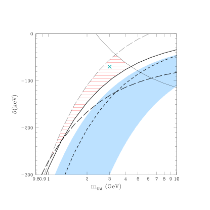
Figure 1: Mass splitting $\delta=m_{\chi^{\prime}}-m_{\chi}$ as a function of $m_{\chi}$. The horizontally (red) hatched area represents the IDM parameter space where the excess measured by CDMS-$Si$cdms_si corresponds to a $v_{min}<v_{esc}^{Lab}$ range which is always below the corresponding one probed by LUX and XENON100 (adapted from noi ). As explained in the text, in this case Xenon experiments can constrain the CDMS-$Si$ excess only when some assumptions are made on the galactic velocity distribution. The enclosed region is the result of the combination of four conditions: the thin solid line where $v_{min}(E^{LUX}_{min})$=$v_{min}(E^{CDMS-Si}_{max})$; the thick solid line where $v_{min}(E^{LUX}_{min})$=$v_{min}(E^{CDMS-Si}_{min})$; the thin long–dashed line where $v_{min}(E^{CDMS-Si}_{max})$=$v_{esc}^{Lab}$; the thick long–dashed line where $v_{min}(E^{CDMS-Si}_{min})$=$v_{esc}^{Lab}$ (see text). The corresponding boundaries for XENON100 are less constraining: in particular the thin short–dashed line represents the parameter space where $v_{min}(E^{XENON100}_{min})$=$v_{min}(E^{CDMS-Si}_{min})$. The blue shaded strip represents points excluded by the consistency test introduced in Section 4.1 of Ref. noi . The cross represents the benchmark point discussed in detail in Section VII.

The CDM-$Si$ experimentcdms_si has observed three WIMP candidate events at energies $E_{R}$=8.2 keVnr, 9.5 keVnr and 12.3 keVnr analyzing the full energy range 7 keVnr$<E_{R}<$100 keVnr with an exposure of 140.2 kg day with a Silicon target. The probability estimated by the same Collaboration that the known backgrounds would produce three or more events in the signal region is 5.4%.

An explanation of the three events observed by CDMS–$Si$ in terms of a WIMP with a scalar isospin–conserving interaction (i.e. the scaling law of Eq. (2)) and assuming an isothermal sphere model for the WIMP velocity distribution in the halo of our Galaxy appears to be in strong disagreement with constraints from at least three experiments: LUXlux , XENON100xenon100 and SuperCDMS super_cdms . As shown by several authors ge_phobic for a light WIMP mass ($m_{\chi}\mathrel{\mathop{\kern 0.0pt\hbox to0.0pt{\raise 0.86108pt\hbox{$<$}\hss}}\lower 3.87495pt\hbox{\kern-1.90002pt$\sim$}}$ 10 GeV) and an exothermic interaction ($\delta<0$) the XENON100 constraint could be evaded, while, in order to reconcile the result with the SuperCDSM bound, Isospin Violation suppressing the WIMP coupling with Germanium targets ($Ge$–phopic exothermic DM) could be advocated. This scenario was however excluded by the subsequent LUX bound with its lower threshold and higher exposure compared to XENON100, if an isothermal sphere is assumed for the WIMP velocity distribution $f(\vec{v})$ in our Galaxy; a halo–independent analysis, however, shows that the CDMS–$Si$ excess and LUX can be compatible noi provided that the isothermal sphere assumption is abandoned and only minimal assumptions are made on $f(\vec{v})$.

Namely, as discussed in detail in noi , when no model is assumed for the velocity distribution, an experiment can conservatively constrain an excess claimed by another one only if it is sensitive to the same $v_{min}$ interval, or to lower values. The latter condition descends from the minimal requirement that the $\tilde{\eta}$ function defined in (9,15) is decreasing monotonically with $v_{min}$ (since $v_{min}$ is the lower bound of an integration of the positive function $f(\vec{v})/|\vec{v}|$). At the same time the requirement that the WIMPs are gravitationally bound to our Galaxy implies that the signal region must verify the condition that $v_{min}<v_{esc}^{Lab}$, with $v_{esc}^{Lab}$ the Galactic escape velocity boosted in the Lab rest frame. The two latter conditions depend on the mapping between $E_{R}$ and $v_{min}$, which, according to Eq.(10), in the IDM scenario can be modified by assuming $\delta\neq$0. In particular, if, for the same choice of $m_{\chi}$ and $\delta$, conflicting experimental results can be mapped into non–overlapping ranges of $v_{min}$ and if the $v_{min}$ range of the constraint is at higher values compared to the excess (while that of the signal remains below $v_{esc}^{Lab}$) the tension between the two results can be eliminated by an appropriate choice of the $\tilde{\eta}$ function. This at the price of having to assume that the function $\tilde{\eta}$ drops to appropriately low values in the (high) $v_{min}$ range pertaining to the constraint.

The result of a similar analysis in the $m_{\chi}$–$\delta$ parameter space is shown in Fig. 1noi . In the case of LUX we have assumed the range 2 PE$\leq S_{1}\leq$30 PE for the primary scintillation signal $S_{1}$ (directly in Photo Electrons, PE) while for XENON100 we have taken the experimental range 3 PE$\leq S_{1}\leq$30 PE. In both cases, following Eqs. (14-15) of Ref. xenon100_response we have modeled the detector’s response with a Poissonian fluctuation of the $S_{1}$ scintillation photoelectrons combined with a Gaussian resolution $\sigma_{PMT}$=0.5 PE for the photomultiplier. In Fig. 1 the horizontally (red) hatched area represents the IDM parameter space where the excess measured by CDMS-$Si$cdms_si corresponds to a $v_{min}<v_{esc}^{Lab}$ range which is always below the corresponding one probed by LUX and XENON100. In Fig. 1 we take $v_{esc}^{Lab}=$782 km/s (by combining the reference value of the escape velocity $v_{esc}^{Galaxy}$=550 km/s in the galactic rest frame with the velocity $v_{0}$=232 km/s of the Solar system with respect to the WIMP halo) and the CDMS–$Si$ signal region is approximated with the energy range 8 keVnr$<E_{R}<$12.5 keVnr.

From direct inspection of Fig.1, indeed exothermic DM (i.e. -260 keV$\mathrel{\mathop{\kern 0.0pt\hbox to0.0pt{\raise 0.86108pt\hbox{$<$}\hss}}\lower 3.87495pt\hbox{\kern-1.90002pt$\sim$}}\delta\mathrel{\mathop{\kern 0.0pt\hbox to0.0pt{\raise 0.86108pt\hbox{$<$}\hss}}\lower 3.87495pt\hbox{\kern-1.90002pt$\sim$}}$ -40 keV) is required to allow compatibility between the CDM–Si excess and bounds from liquid–Xenon scintillators, as well as very low values of the WIMP particle mass ($m_{\chi}\mathrel{\mathop{\kern 0.0pt\hbox to0.0pt{\raise 0.86108pt\hbox{$<$}\hss}}\lower 3.87495pt\hbox{\kern-1.90002pt$\sim$}}$ 4 GeV). Indicating the Region of Interest of each experiment by $[E_{min},E_{max}]$, in Fig.1 several curves are shown: on the thin solid line $v_{min}(E^{LUX}_{min})$=$v_{min}(E^{CDMS-Si}_{max})$; on the thick solid line $v_{min}(E^{LUX}_{min})$=$v_{min}(E^{CDMS-Si}_{min})$; the thin long–dashed line corresponds to $v_{min}(E^{CDMS-Si}_{max})$=$v_{esc}^{Lab}$; the thick long–dashed line to $v_{min}(E^{CDMS-Si}_{min})$=$v_{esc}^{Lab}$. The corresponding boundaries for XENON100 are less constraining: in particular the thin short–dashed line represents the parameter space where $v_{min}(E^{XENON100}_{min})$=$v_{min}(E^{CDMS-Si}_{min})$. The blue shaded strip represents points excluded by the consistency test introduced in Section 4.1 of Ref. noi , and does not affect the compatibility region.

The same check can be made between the CDMS–$Si$ excess and the SuperCDMS experiment boundsuper_cdms , but in this case no analogous compatibility region can be found in all the $m_{\chi}$–$\delta$ plane. This means that, besides experimental issues, the two measurements cannot be reconciled using kinematics arguments only. However, in presence of some additional dynamical mechanism suppressing WIMP scatterings on Germanium compared to that on Silicon, the CDMS–$Si$ result and the SuperCDMS bound can in principle be reconciled. An example of such mechanism is the ”$Ge$–phobic” IVDM scenario which is the main subject of the present analysis.

In Section VII we will adopt the benchmark point represented by a cross in Fig.1 to perform a full numerical analysis of the IVDM parameter space.

IV.1 From direct–detection data to suppression scale

Following the halo–independent procedure outlined in Section II.1 it is straightforward, for a given choice of the DM parameters, to obtain estimations $\bar{\tilde{\eta}}_{i}^{CDMS-Si}$ of the function $\tilde{\eta}(v_{min})$ averaged in appropriately chosen $v_{min}$ intervals mapped from the CDMS–Si Region of Interest (see Eq.(19)). Notice that, in order to do so, along with $m_{\chi}$ and $\delta$ also the scaling law (either given by Eq.(14) or Eq. (30)) is required. According to the discussion above, in the Isospin–Conserving case (i.e. for the scaling law of Eq.(2)) the upper bounds $\bar{\tilde{\eta}}_{i,lim}^{SuperCDMS}$ from SuperCDMS in the same $v_{min}$ ranges are well below the $\bar{\tilde{\eta}}_{i}^{CDMS-Si}$ estimations, so that, at face value and barring other issues such as experimental systematic errors, an explanation of the CDMS–Si effect in terms of WIMP scatterings is in strong tension with the available data. However, as discussed in Section III, an appropriate choice of the parameters $\bar{\lambda}_{q},\bar{\lambda}_{\theta}$ can suppress the expected rate on Germanium compared to that on Silicon, driving the $\bar{\tilde{\eta}}_{i,lim}^{SuperCDMS}$ constraints above the $\bar{\tilde{\eta}}_{i}^{CDMS-Si}$ estimations. Quantitatively, the compatibility between the two results can be assessed introducing the following compatibility ratio:

$${\cal D}(m_{\chi},\delta,\bar{\lambda}_{d},\bar{\lambda}_{s},\bar{\lambda}_{\theta})\equiv\max_{i\in\mbox{signal}}\left(\frac{\bar{\tilde{\eta}}_{i}^{CDMS-Si}+\sigma_{i}}{\min_{j\leq i}\bar{\tilde{\eta}}_{j,lim}}\right),$$ (33)

where $\sigma_{i}$ represents the standard deviation on $\bar{\tilde{\eta}}_{i}^{CDMS-Si}$ as estimated from the data, $i\in\mbox{signal}$ means that the maximum of the ratio in parenthesis is for $v_{min,i}$ corresponding to the CDMS–$Si$ excess, while, due to the fact that the function $\tilde{\eta}$ is non–decreasing in all velocity bins $v_{min,i}$, the denominator contains the most constraining bound on $\tilde{\eta}$ for $v_{min,j}\leq v_{min,i}$. The latter minimum includes all available bounds, although, in practice, only Super–CDMS will prove to be effective in the discussion of Section VII. Specifically, compatibility between CDMS–Si and all other experiments (including SuperCDMS) is ensured if ${\cal D}<$1: in this case all the 1–$\sigma$ ranges of the $\bar{\tilde{\eta}}_{i}^{CDMS-Si}$’s are below the upper bounds from other experiments with $v_{min}\leq v_{min,i}$. Notice that the definition above combines different $v_{min,i}$ bins, allowing for some energy–dependence in the scaling law (as suggested by Eqs.(26) and (27)). On the other hand, if only one target is relevant for the constraint and in the LO case, or if the energy dependence is neglected in the NLO case, the ratio between the scaling laws corresponding to Silicon and the target element of the bound factors out in the sum above. In this case ${\cal D}$ is a function of $\bar{\lambda}_{d}$,$\bar{\lambda}_{s}$,$\bar{\lambda}_{\theta}$ only through particular combinations (the $r=f_{n}/f_{p}$ parameter in the LO case or the $t$ parameter defined in Eq.(31)). However, if the scaling law depends on the energy, all the three ratios $\bar{\lambda}_{d}$,$\bar{\lambda}_{s}$,$\bar{\lambda}_{\theta}$ are needed to calculate ${\cal D}$. In the former case ${\cal D}$ can be minimized as a function of $r$ or $t$ and its minimum value ${\cal D}_{min}$ is constant in the plane $\bar{\lambda}_{s}$–$\bar{\lambda}_{\theta}$ (although each point will correspond to a different value of $\bar{\lambda}_{d,min}$). In the latter case ${\cal D}(\bar{\lambda}_{d},\bar{\lambda}_{s},\bar{\lambda}_{\theta})$ can be minimized as a function of $\bar{\lambda}_{d}$ at fixed $\bar{\lambda}_{s}$ and $\bar{\lambda}_{\theta}$. We will proceed in this way in the numerical analysis of Section VII.

We also notice here that the $\bar{\tilde{\eta}}_{i}^{CDMS-Si}$ values determined from the data must be compatible with the property that the $\tilde{\eta}$ function is decreasing with $v_{min}$. A possible criterion to quantify this condition is that the lower range of each $\bar{\tilde{\eta}}_{i+1}^{CDMS-Si}$ falls below the upper range of the $\bar{\tilde{\eta}}_{i}^{CDMS-Si}$ with immediately lower $v_{min}$, i.e.:

$${\cal R}=\max_{i\in\mbox{signal}-1}\frac{\bar{\tilde{\eta}}_{i+1}^{CDMS-Si}-\sigma_{i+1}}{\bar{\tilde{\eta}}_{i}^{CDMS-Si}+\sigma_{i}}<1.$$ (34)

Combining conditions (33) and (34), full compatibility is achieved if $\max({\cal D},{\cal R})<1$. In practice, due to the low statistics of the CDMS–Si excess and the ensuing large error bars on the $\bar{\tilde{\eta}}_{i}^{CDMS-Si}$, ${\cal R}$ is always less than 1 and only the condition (33) will turn out to be effective (see for instance Fig.5).

Once the $m_{\chi}$, $\delta$, $\bar{\lambda}_{d}$, $\bar{\lambda}_{s}$, $\bar{\lambda}_{\theta}$ parameters are fixed, the value of the suppression scale $\tilde{\Lambda}$ required to explain the $\bar{\tilde{\eta}}_{i}^{CDMS-Si}$ obtained from the CDMS–Si data should be estimated in order to get information on the underlying DM model. This requires to determine the cross section $\sigma_{0}$ from Eq.(15), disentangling particle physics form astrophysics, and is not possible without specifying the velocity distribution $f(\vec{v})$. However, since $\int f(\vec{v})d^{3}v$=1, the function $\eta(v_{min})$ can be at least maximized by the choice $f(\vec{v})=\delta(v_{s}-v_{min})$, with $v_{s}$ the maximal value of the $v_{min}$ range corresponding to the CDMS–Si excess. This corresponds to the largest $\eta(v_{min})$ which does not vanish in the signal range. In this case:

$$\tilde{\eta}^{max}(v_{min})=\bar{\tilde{\eta}}_{fit}^{CDMS-Si}\theta(v_{s}-v_{min}).$$ (35)

Notice that the large error bars on the $\bar{\tilde{\eta}}_{i}^{CDMS-Si}$ imply that, indeed, the above ensuing flat functional form for the $\tilde{\eta}$ function is not incompatible with the data. The constant value $\bar{\tilde{\eta}}_{fit}^{CDMS-Si}$ can then the be fitted from the data in a straightforward way. Plugging Eq.(35) in Eq.(15) and using for $\sigma_{0}$ the expression given in Eq.(12), one gets:

$$\tilde{\Lambda}=f_{0}^{\frac{1}{3}}\left(\frac{2\rho_{\chi}\mu_{\chi p}^{2}}{\pi\bar{\tilde{\eta}}_{fit}^{CDMS-Si}m_{\chi}v_{s}}\right)^{\frac{1}{6}}.$$ (36)

Obviously $\tilde{\Lambda}$ does not depend on choice of the arbitrary amplitude $f_{0}$ chosen for the factorization, since $\bar{\tilde{\eta}}_{fit}^{CDMS-Si}$ is fitted using the scaling law (14) and scales with $f_{0}^{2}$.

Notice than in Eq.(4) for dimensional reason the suppression scale $\Lambda$ appears at the third power having extracted a quark mass factor from the coupling. We followed this convention to comply to that of Ref. isospin_violation_nlo2 . An alternative way to parametrize the same interaction is to write the Lagrangian in the form:

$${\cal L}=\sum_{q=u,d,s,c,b,t}\frac{\tilde{\xi}_{q}}{M_{*}^{2}}\bar{\chi}^{\prime}\chi\bar{q}q\mbox{+h.c.}.$$ (37)

Lacking a knowledge of the ultraviolet completion of the model both forms are acceptable. However, since $m_{q}/\Lambda\ll$1, numerically $M_{*}\gg\Lambda$ for the same values of the expected signals, so in order to get an upper bound on the scale of the new physics involved in the process we chose to discuss constraints on $M_{*}$. In particular this can be done by imposing the perturbativity condition:

$$\max(|\tilde{\xi}_{q}|)\leq 4\pi,$$ (38)

which implies:

$$M_{*}\leq\sqrt{4\pi}\tilde{\Lambda}\left(\frac{\tilde{\Lambda}}{\mbox{max($m_{q}\bar{\lambda}_{q}$)}}\right)^{\frac{1}{2}},$$ (39)

with $\tilde{\Lambda}$ given by Eq.(36).

The procedure outlined above will be adopted In Section VII to get an estimation of the maximal value of $M_{*}$.

V Relic abundance

A minimal necessary requirement of the exothermic DM scenario (i.e. $\delta<0$) is that the metastable $\chi$ particle decays to the lower–mass state $\chi^{\prime}$ on a time scale larger than the age of the Universe. Specifically, the effective Lagrangian of Eq.(4) drives the decay $\chi\rightarrow\chi^{\prime}\gamma\gamma$, whose amplitude has been recently estimated making use of Chiral Perturbation Theory decay :

$$\Gamma\simeq\frac{B_{0}^{2}\alpha_{EM}^{2}}{32(105\pi^{5})\Lambda_{c}^{4}\tilde{\Lambda}^{6}}\left|m_{u}\tilde{\lambda}_{u}-m_{d}\tilde{\lambda}_{d}\right|^{2}\delta^{7},$$ (40)

with $B_{0}=m_{\pi}^{2}/(m_{u}+m_{d})$, $\Lambda_{c}\simeq 4\pi f_{\pi}/\sqrt{N}$, $N=2$, $f_{\pi}$=93 MeV and $m_{\pi}$ the pion mass. As discussed in decay , the range of the $\delta$ parameter involved in direct detection ($|\delta|\mathrel{\mathop{\kern 0.0pt\hbox to0.0pt{\raise 0.86108pt\hbox{$<$}\hss}}\lower 3.87495pt\hbox{\kern-1.90002pt$\sim$}}$ 100 keV) drives the amplitude (40) to values safely below that corresponding to the age of the Universe, $\tau_{U}^{-1}\simeq 1.5\times 10^{-42}$ GeV . This will be confirmed by the quantitative analysis of Section VII.

As far as the production mechanism for the $\chi$ particle cosmological density is concerned, several can be devised. Thermal decoupling, where the particles $\chi$ and $\chi^{\prime}$ are initially in thermal equilibrium in the plasma of the Early Universe until their interactions freeze-out at a temperature $T\simeq m_{\chi}/20$, is the most standard and predictive. One can notice that the mass splitting involved ($|\delta|\mathrel{\mathop{\kern 0.0pt\hbox to0.0pt{\raise 0.86108pt\hbox{$<$}\hss}}\lower 3.87495pt\hbox{\kern-1.90002pt$\sim$}}$ 100 keV) is much smaller than the typical freeze–out temperature even for very light WIMPs, $T_{f}\simeq m_{\chi}/20\mathrel{\mathop{\kern 0.0pt\hbox to0.0pt{\raise 0.86108pt\hbox{$>$}\hss}}\lower 3.87495pt\hbox{\kern-1.90002pt$\sim$}}$ 50 MeV for $m_{\chi}\mathrel{\mathop{\kern 0.0pt\hbox to0.0pt{\raise 0.86108pt\hbox{$>$}\hss}}\lower 3.87495pt\hbox{\kern-1.90002pt$\sim$}}$ 1 GeV. As a consequence of this the chemical potential between the $\chi$ and $\chi^{\prime}$ states can be safely neglected, and the corresponding number (and mass) densities $n_{\chi}$ and $n_{\chi^{\prime}}$ of both species should be the same when they decouple at $T=T_{F}$. This is also true below $T_{F}$ when, as long as $T\mathrel{\mathop{\kern 0.0pt\hbox to0.0pt{\raise 0.86108pt\hbox{$>$}\hss}}\lower 3.87495pt\hbox{\kern-1.90002pt$\sim$}}\delta$, kinetic equilibrium is maintained by the reactions $\chi+q\leftrightarrow\chi^{\prime}+q$ (below the QCD–phase transition, $T_{QCD}\simeq 150$ MeV, these reactions will briefly involve pions until the latter become non–relativistic and their density drops exponentially). The bottom line is that, being $\chi^{\prime}$ stable on cosmological scales, the condition $n_{\chi}$=$n_{\chi^{\prime}}$ is likely to be maintained until the present day, so that, in this scenario, galactic halos contain equal densities of $\chi$ and $\chi^{\prime}$. In principle this implies that direct detection experiments should be able to measure at the same time $\chi$ down–scatters to $\chi^{\prime}$ and $\chi^{\prime}$ up–scatters to $\chi$. However, we notice that, as discussed in Section IV, if exothermic DM is advocated to explain the three WIMP candidates in CDMS–$Si$, very low WIMP masses are required, $m_{\chi}\mathrel{\mathop{\kern 0.0pt\hbox to0.0pt{\raise 0.86108pt\hbox{$<$}\hss}}\lower 3.87495pt\hbox{\kern-1.90002pt$\sim$}}$ 4 GeV, as well as $\delta\mathrel{\mathop{\kern 0.0pt\hbox to0.0pt{\raise 0.86108pt\hbox{$<$}\hss}}\lower 3.87495pt\hbox{\kern-1.90002pt$\sim$}}-50$ keV noi . In this case Eq. (10 ) implies that up-scatters ($\delta>0$) are only possible when the incoming WIMP velocity (in the Earth’s rest frame) is larger than the minimal value $v_{min}=v_{*}=\sqrt{2\delta/\mu_{\chi N}}\simeq\sqrt{2\delta/m_{\chi}}\mathrel{\mathop{\kern 0.0pt\hbox to0.0pt{\raise 0.86108pt\hbox{$>$}\hss}}\lower 3.87495pt\hbox{\kern-1.90002pt$\sim$}}$ 950 km/s, a value incompatible to acceptable values of the galactic escape velocity (in Section IV we adopt the reference value $v_{esc}^{Lab}\simeq$ 782 km/s). So, in this particular scenario, only down–scatters are detectable, and this implies that strictly speaking, if $\rho_{DM}=\rho_{\chi}+\rho_{\chi^{\prime}}$ is the DM density estimated in the neighborhood of the Sun by its gravitational interactions, the incoming WIMP flux to which all direct detection experiments are sensitive is proportional to only half of that, $\rho_{DM}/2$.

As in the elastic casecdms_si_eff ; cdms_si_eff2 , the coannihilation cross section for the process $\chi\chi^{\prime}\rightarrow qq$ at decoupling is velocity–suppressed for a scalar interaction because in $s$–wave the $\chi\chi^{\prime}$ system has parity -1. As a consequence, if the typical scale $\tilde{\Lambda}$ required to explain the CDMS–Si excess is used to calculate the relic abundance, too large values incompatible to observation are found cdms_si_eff . This will be generally confirmed by the phenomenological analysis of Section VII. However, as shown in the previous Section, in the isospin–violating scenario the regions of the ($\bar{\lambda}_{\theta}$–$\bar{\lambda}_{s}$) parameter space close to Eq.(25) or Eq. (32) correspond to large cancellations among the coupling constants $\tilde{\lambda}_{q}$ in the calculation of the direct detection rate, which drive the suppression scale $\tilde{\Lambda}$ to values significantly lower than in the isospin–conserving case for a fixed number of predicted events. On the other hand, in the calculation of the coannihilation cross section that fixes the thermal relic abundance only the absolute values of the coupling constants $|\tilde{\lambda}_{q}|^{2}$ appear:

$$<\sigma v> = \frac{3m_{\chi}^{2}}{8\pi\Lambda^{6}}\sum_{q}m_{q}^{2}\left|\tilde{\lambda}_{q}\right|^{2}\left(1-\frac{m_{q}^{2}}{m_{\chi}^{2}}\right)^{\frac{3}{2}}\times$$ (41)

$$\left(6x^{-1}-27x^{-2}+...\right),$$

so that no cancellation is at work to compensate the enhancement due to a small $\tilde{\Lambda}$. As we will see, this represents a possible mechanism to drive the thermal relic abundance down to values compatible to observation also for a scalar–type interaction, at variance with the Isospin–conserving case. In Eq.(41) $x\equiv m_{\chi}/T$, and we have neglected the mass splitting between $\chi$ and $\chi^{\prime}$ taking $m_{\chi}^{\prime}$=$m_{\chi}$ since $\delta\ll T_{f}\simeq m_{\chi}/20$. Below $T_{f}$ the total relic density of $\chi$ and $\chi^{\prime}$ freezes to the usual value:

$$\Omega h^{2}\simeq\frac{8.7\times 10^{-11}/\mbox{GeV${}^{2}$}}{g_{*}^{1/2}(x_{f})}\frac{1}{\int_{0}^{x_{f}}<\sigma v>dx},$$ (42)

where $g_{*}(x_{f})$ denotes the number of relativistic degrees of freedom of the thermodynamic bath at $x_{f}$.

VI Signals at the LHC

We have simulated monojet+missing transverse energy $\not\!E_{T}$ monojet_theory ; monojet_exp and hadronically–decaying mono $W/Z$ eventsmono_wz_theory ; atlas_wz at the LHC in $pp$ collisions at $\sqrt{s}$ = 8 TeV using MadGraph 5 madgraph , interfaced with Pythia 6 pythia and Delphes 3 delphes , with the scalar interaction of Eq.(4), using CTEQ6L1 Parton Distribution Functions cteq6l1 and including the $b$ quark. Notice that in collider physics the effect of the mass splitting between $\chi$ and $\chi^{\prime}$ is completely negligible.

As far as the monojet signal is concerned, we have required the transverse momentum $P_{t}$ of each parton to be larger than 80 GeV pt_jet and applied the following kinematic cuts at the detector level cdms_si_eff2 :

• $p_{T_{j}}>$ 110 GeV, with $p_{T_{j}}$ the jet transverse momentum;

• $|\eta_{j}|<$ 2.4, with $|\eta_{j}|$ the jet pseudorapidity;

• $\not\!E_{T}>$ 400 GeV.

In the case of hadronically–decaying mono $W/Z$ events, we calculate the total production cross section, applying the same cuts used in atlas_wz :

• $p^{W,Z}_{T}>$ 250 GeV, where $p^{W,Z}_{T}$ is the $W$ or $Z$ transverse momentum;

• $|\eta|^{W,Z}<$ 1.2, where $\eta^{W,Z}$ is the pseudo-rapidity;

• $\sqrt{y}>$ 0.4, where $\sqrt{y}\equiv\min(p^{T}_{1},p^{T}_{2})\Delta R/m_{jet}$, with $p^{T}_{i}$ (i = 1 or 2) being the transverse momentum of the two leading reconstructed jets from the $W$ or $Z$ decay, $\Delta R$=$\sqrt{(\Delta\eta)^{2}+(\Delta\phi)^{2}}$ the distance in pseudo–rapidity and azimuthal angle between jets, and $m_{jet}$ the jets invariant mass.

• $P^{T}_{\chi\chi^{\prime}}>$ 350 GeV, with $P^{T}_{\chi\chi^{\prime}}$ the invisible transverse momentum carried away by the $\chi$, $\chi^{\prime}$ particles.

In both analyzes we have used the anti–kt jet–reconstruction algorithm with parameter $R$=0.5.

VII Discussion

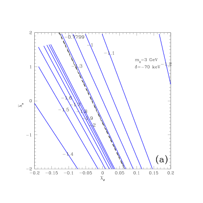
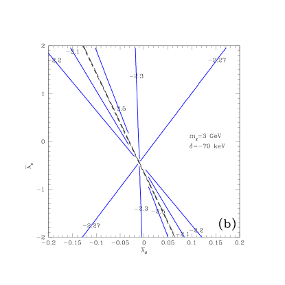
Figure 2: Isospin–violation parameter space for $m_{\chi}$=3 GeV and $\delta$=-70 keV (IDM benchmark point indicated with a (green) cross in Fig. 1). For each value of $\bar{\lambda}_{\theta}$ and $\bar{\lambda}_{s}$ the remaining parameter $\bar{\lambda}_{d}$ is set to the value $\bar{\lambda}_{d,min}$ minimizing the quantity ${\cal D}$ defined in Eq. (33). (a) The solid lines show constant values of $r=f_{n}/f_{p}=r_{min}$, i.e. the value of $r$ that minimizes the compatibility ratio ${\cal D}$. (b) The solid lines show constant values of $t=t_{min}$, i.e. the value of the $t$ parameter introduced in Eq. (31) that minimizes the compatibility ratio ${\cal D}$. In both figures the NLO corrections of Eq. (26) are included, while the short–dashed and long dashed straight lines represent the “alignment” conditions given in Eqs.(25) and (32), respectively.

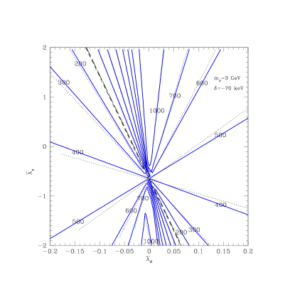
Figure 3: Same as in Fig. 2. On the solid lines the upper bound on the suppression scale $M_{*}$ (introduced in Eq.(39)) is fixed to the indicated value when the NLO corrections of Eq. (26) to the expected WIMP rate are included. Dashed lines represent the same for the LO calculation.

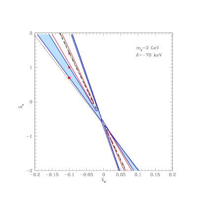
Figure 4: Same as in Fig.2. The shaded regions are bounded by the solid blue lines corresponding to the two conditions $\Omega_{\chi}h^{2}$=0.12 and ${\cal D}_{min}$=1 and represent the parameter space where CDMS–Si and SuperCDMS are mutually compatible while at the same time the metastable state $\chi$ can be a thermal relic (i.e. $\Omega_{\chi}h^{2}\leq$0.12 using Eq. (42)). The dotted curve represents the condition $\Omega_{\chi}h^{2}$=0.12 calculated using the LO scaling law for the expected rate (see Eq.(6). Finally, the inner solid (red) line corresponds to $\tau=1/\Gamma$=4$\times$10²⁶ seconds, as given by Eq.(40). The (red) circle indicates the representative choice of $\bar{\lambda}_{\theta}$, $\bar{\lambda}_{s}$ shown in Fig.5(a) for which $\Omega_{\chi}h^{2}$=0.12, which corresponds to ${\cal D}_{min}$=0.7; the square indicates the choice of $\bar{\lambda}_{\theta}$, $\bar{\lambda}_{s}$ shown in Figs.5(b) 6(a) and for which ${\cal D}_{min}$=1 (i.e. at the verge of incompatibility between the CDMS–Si result and the SuperCDMS constraint); the (red) triangle indicates the representative choice of $\bar{\lambda}_{\theta}$, $\bar{\lambda}_{s}$ shown in Figs.6(b), and exemplifies a configuration very close to Eq.(32) where the NLO energy–dependent corrections of Eq. (26) spoil the maximal achievable cancellation in WIMP–$Ge$ scattering.

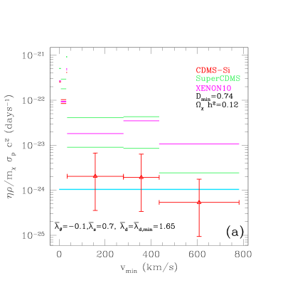
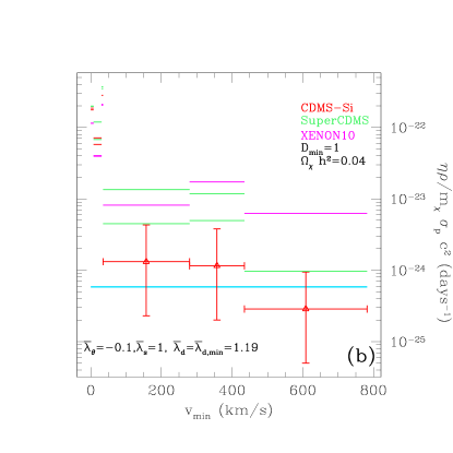
Figure 5: Measurements and bounds for the function $\tilde{\eta}$ defined in Eq.(15) for $\sigma_{0}=\sigma_{p}$ and $m_{DM}$=3 GeV, $\delta$=-70 keV, i.e. for the IDM benchmark point indicated with a (green) cross in Fig. 1. (a) $\bar{\lambda}_{\theta}$=-0.1, $\bar{\lambda}_{s}$=0.7 (benchmark point indicated with a circle in Fig.4, corresponding to $\Omega_{\chi}h^{2}$=0.12). (b) $\bar{\lambda}_{\theta}$=-0.1, $\bar{\lambda}_{s}$=1 (benchmark point indicated with a square in Fig.4 and corresponding to ${\cal D}_{min}$=1). In both figures $\bar{\lambda}_{d}$=$\bar{\lambda}_{d,min}$ minimizes the ${\cal D}$ function of Eq. (33) and the thick (blue) horizontal line represents the quantity $\bar{\tilde{\eta}}_{fit}^{CDMS-Si}$ introduced in Eq. (35). Note that, consistently with the condition ${\cal D}_{min}$=1, in plot (b) the constraint from SuperCDMS “touches” the upper range of the CDMS–$Si$ excess.

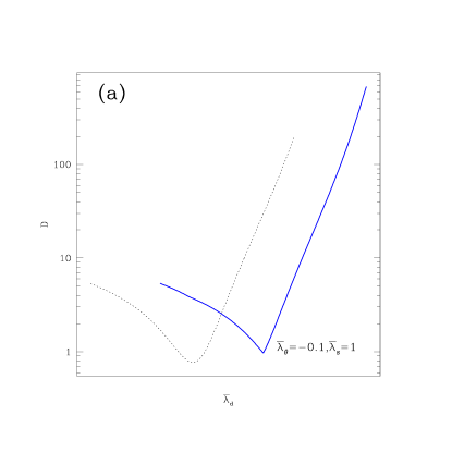
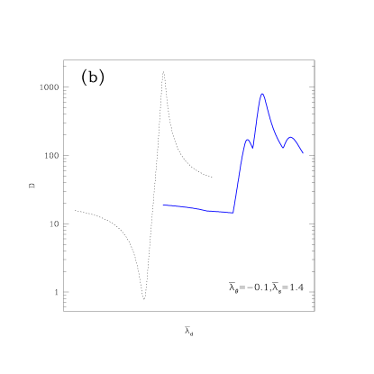
Figure 6: The compatibility ratio ${\cal D}$ defined in Eq.(33) is plotted as a function of $\bar{\lambda}_{d}$ for $m_{DM}$=3 GeV, $\delta$=-70 keV, i.e. for the IDM benchmark point indicated with a (green) cross in Fig. 1.(a) $\bar{\lambda}_{\theta}$=-0.1, $\bar{\lambda}_{s}$=1 (benchmark point indicated with a (red) square in Fig.(4)). (b) $\bar{\lambda}_{\theta}$=-0.1, $\bar{\lambda}_{s}$=1.4 (benchmark point indicated with a (red) triangle in Fig.(4)). In both figures the solid (blue) line represents the calculation including the NLO corrections of Eq. (26), while the thin dotted (black) line shows the same quantity when the approximate expression for the NLO corrections of Eq.(29) is used, which neglects the terms with explicit energy dependence.

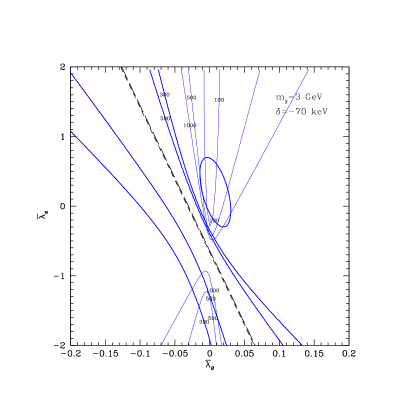
Figure 7: Same as in Fig.2. The thick solid lines show constant values of the cross section for hadronically–decaying mono $W/Z$ events in $fb$, while thin solid lines represent constant values of the expected number of monojet+missing energy events for the integrated luminosity ${\cal L}$=19.5 $fb^{-1}$. In both cases $\sqrt{s}$=8 TeV. The applied kinematic cuts are listed in Section VI.

In the following we will assume that the CDMS–$Si$ effect is explained in terms of a WIMP signal, and we will fix the IDM parameters to the benchmark $m_{\chi}$=3 GeV, $\delta$=-70 keV (indicated by a cross in Fig. 1). As already explained, this choice of parameters is kinematically not accessible to XENON100 and LUX, but is covered by SuperCDMS noi , so that the Isospin Violation mechanism must be advocated to suppress WIMP scattering on $Ge$ targets compared to $Si$, or, quantitatively, minimizing the compatibility ratio ${\cal D}$ introduced in Eq.(33). In order to calculate the latter, in our analysis we will fix the following three energy bins for CDMS-$Si$, each containing one of the WIMP candidate events: 7.4 keVnr$\leq$8.2 keVnr, 8.2 keVnr$\leq$9.5 keVnr, 9.5 keVnr$\leq$12.3 keVnr. We will then map them through $v_{min}$ into energy ranges for SuperCDMS, for which we use the low–energy analysis of Ref.super_cdms with a Germanium target in the energy range 1.6 keVnr$<E_{R}<$ 10 keVnr with a total exposition of 577 kg day and 11 observed WIMP candidates. Since the energy resolution in CDMS-$Si$ has not been measured, we take for both CDMS-$Si$ and SuperCDMS $\sigma_{CDMS-Si}(E^{\prime})=\sqrt{0.293^{2}+0.056^{2}(E^{\prime}/\mbox{keVnr})}$ in keVnr from cdms_resolution . As already pointed out, the definition of ${\cal D}$ includes in principle all available bounds (also for the $v_{min}$ range below that corresponding to the CDMS–$Si$ effect). Specifically the kinematic regime we are interested in is also probed by XENON10. The latter makes use of the secondary ionization signal $S_{2}$ only, with an exposition of 12.5 day and a fiducial mass of 1.2 kg. In the following we have included XENON10 in our numerical calculation of ${\cal D}$, although we have found that only Super–CDMS is relevant to the discussion, since XENON10 does not imply any constraint (see for instance Fig.5). In particular, for XENON10 we have taken the scale of the recoil energy $E_{R}$ and the recorded event spectrum in the energy range 1.4 keVnr$<E_{R}<$ 10 keVnr directly from Fig. 2 of Ref. xenon10 , while for the energy resolution we have assumed $\sigma_{XENON10}=E_{R}/\sqrt{E_{R}Q_{y}(E_{R})}$ where $Q_{y}(E_{R})$ is the electron yield that we calculated with the same choice of parameters as in Fig. 1 of xenon10 .

When the LO expression (6) is used for the WIMP expected rate, ${\cal D}$ is minimized by $r=f_{n}/f_{p}\simeq-0.78$isospin_violation . This situation is modified when NLO corrections to the scattering rate (see Eq.(26)) are included. This is shown in Fig 2(a), where the solid lines represent constant values of $r=f_{n}/f_{p}=r_{min}$, corresponding to ${\cal D}_{min}$ when the NLO expression (26) is used instead. Indeed, values as small as -2 are now possibleisospin_violation_nlo2 . As already pointed out, this is due to the fact that the cancellation in this case is no longer between the WIMP couplings to protons and neutrons, but between the latter ad the two–nucleon amplitude given in the last of Eqs.(27). In the same figure the short–dashed and long dashed straight lines represent the “alignment” conditions given in Eqs.(25) and (32), respectively. As discussed in Section III.2, close to these straight lines the WIMP expected rate vanishes for all targets at the same time, so that, strictly speaking, the compatibility ratio ${\cal D}$ cannot be minimized in the first place. In practice close to those lines the $r_{min}$ parameter is subject to large numerical oscillation when ${\cal D}$ is minimized.

As pointed out in Section III.2, however, the most relevant quantity from the phenomenological point of view is the minimal achievable value ${\cal D}_{min}$ of the ${\cal D}$ ratio, which in the NLO case is not driven by the $r$ parameter, but instead by the $t$ parameter defined by the scaling law recast as in Eq.(31). Indeed, when the energy–dependent terms in the NLO corrections of Eq.(27) are neglected, ${\cal D}$ is minimized to the same value ${\cal D}_{min}$ of the LO case, albeit for a value of the $t$ parameter, $t_{min}\simeq-\bar{A}/Z$, which corresponds to a different value of $r$ in each point of the parameter space. This is shown if Fig.2(b), where the solid lines represent constant values of $t_{min}$ when the full NLO corrections (27) are included. From this figure one can see that indeed, in large parts of the parameter space, $t_{min}$ is very close to the constant value $\simeq-2.3$. The only exception is close to the long-dashed straight line correspondent to Eq.(32), where the energy–independent part of the amplitude cancels out so that the energy–dependent corrections can no longer be neglected: it is this effect that leads to the fluctuations in the values of $t_{min}$ found by the ${\cal D}$ minimization procedure. Notice that the energy dependence of the scaling law is also expected to spoil the cancellation in the ${\cal D}$ minimization leading to higher values of ${\cal D}_{min}$ and in this way playing against the possibility to make CDMS–$Si$ and SuperCDMS mutually compatible. This will be confirmed by our numerical analysis.

As discussed in Section III, the parameter space close to the line of Eq.(25) or Eq.(32) has also another important feature: thanks to the factorization (24), for a given target nucleus the degrading factor (21) can become arbitrarily small, even in presence of many isotopes, so that, if the expected WIMP rate is fixed to explain CDMS–Si, the correspondent scale $M_{*}$ is driven to its smallest values. This is confirmed by Fig.3, where the solid lines show constant values of $M_{*}$, calculated using Eqs.(36,39) with $\rho_{\chi}$=$\rho_{local}$/2, with $\rho_{local}$=0.3 GeV/cm³ (notice that we divide $\rho_{local}$ by two to be consistent with the discussion of Section V, where a scenario with equal densities for the two states $\chi$ and $\chi^{\prime}$ is outlined in which direct detection experiments are only sensitive to $\chi$ down–scatters). As shown in Fig.3, indeed the smallest values for $M_{*}$ are reached close to the straight line (32). This suppression mechanism of $M_{*}$ is expected to enhance both the annihilation cross section of Eq.(41) and the LHC signals: we wish now to analyze this in detail combining the discussion of the direct detection signal (Section IV.1) with the relic abundance calculation (Section V) and signals at the LHC (Section VI).

The Lagrangian of Eq. (4) depends on the 6 couplings $\tilde{\lambda}_{q}$ ($q=u,d,s,c,b,t$) and, as discussed in Section II, the phenomenology is expected to depend on the five ratios $\tilde{\lambda}_{q}/\tilde{\lambda}_{u}$ ($q=d,s,c,b,t$). At variance with the other observables, however, direct detection is sensitive to scales much lower than that of heavy quarks, so that the latter are integrated out and only enter in the calculation of the expected rate through the combination $\lambda_{\theta}$=2/27$\sum_{Q=c,b,t}\tilde{\lambda}_{Q}$. This implies that in each point of the plane $\bar{\lambda}_{\theta}$–$\bar{\lambda}_{s}$ only the sum of heavy-quark couplings is fixed by direct detection, while, in order to calculate other observables, all the couplings $\tilde{\lambda}_{Q}$ are needed. Notice, however, that our choice of the IDM parameters corresponds to $m_{\chi}$,$m_{\chi^{\prime}}$ $\mathrel{\mathop{\kern 0.0pt\hbox to0.0pt{\raise 0.86108pt\hbox{$<$}\hss}}\lower 3.87495pt\hbox{\kern-1.90002pt$\sim$}}m_{b}$. This means that in the annihilation cross section $<\sigma v>$ only the annihilation channels $u\bar{d}$, $d\bar{d}$, $s\bar{s}$ and $c\bar{c}$ are kinematically accessible. As already mentioned in Section V, in the isospin–conserving case the Lagrangian of Eq.(4) leads to a $p$–wave, velocity–suppressed $<\sigma v>$ that drives the thermal relic abundance above the observational constraints. In the following we wish to explore the possibility that the IVDM mechanism may instead allow to find values of the thermal relic abundance compatible to observation, so that we are interested in maximizing $<\sigma v>$. In light of this, in the following we will fix $\tilde{\lambda}_{b}$=$\tilde{\lambda}_{t}$=0, so that in each point of our parameter space $\tilde{\lambda}_{c}$=27/2 $\lambda_{\theta}$.

The result of a combined analysis of the relic abundance and of the minimum compatibility ratio ${\cal D}_{min}$ between CDMS–Si and SuperCDMS is shown in Figs. 4, 5 and 6. Figure 4 shows the $\bar{\lambda}_{\theta}$–$\bar{\lambda}_{s}$ parameter space, where again the short–dashed and long dashed straight lines represent Eqs.(25) and (32), respectively. In this Figure the shaded regions represent the parameter space where CDMS–Si and SuperCDMS are mutually compatible while at the same time the metastable state $\chi$ can be a thermal relic (i.e. $\Omega_{\chi}h^{2}\leq$0.12 using Eq. (42)) and are bounded by the solid blue lines which correspond to the two conditions $\Omega_{\chi}h^{2}$=0.12 and ${\cal D}_{min}$=1. Here in the evaluation of ${\cal D}$ the expected WIMP signal has been calculated using Eq.(26), i.e. including the NLO corrections of Ref.isospin_violation_nlo ; isospin_violation_nlo2 . The existence of such a region in the parameter space, close to the values fixed by Eq.(32) but not overlapping them, is the main result of our analysis. In the same figure the dotted curve represents $\Omega_{\chi}h^{2}$=0.12 calculated using the LO scaling law for the expected rate (see Eq.(6)). This curve is only marginally modified compared to the LO case and confirms what we already pointed out: with very few exceptions the phenomenology is only slightly modified by NLO corrections in spite of the fact that $r_{min}$ can be sizeably changed. Finally, the inner solid (red) line corresponds to $\tau=1/\Gamma$=4$\times$10²⁶ seconds, as given by Eq.(40): indeed for such low values of the $|\delta|$ parameter decay the lifetime of the metastable state $\chi$ is much larger than the age of the Universe, $\tau_{U}\simeq 4.35\times 10^{17}$ seconds. In Figure 4 the (red) circle indicates the representative choice of $\bar{\lambda}_{\theta}$, $\bar{\lambda}_{s}$ for which measurements and bounds for the function $\tilde{\eta}$ defined in Eq.(15) with $\sigma_{0}=\sigma_{p}$ are shown in detail in Fig.5(a). This choice corresponds to $\Omega_{\chi}h^{2}$=0.12 and ${\cal D}_{min}$=0.7. On the other hand, the (red) square indicates the choice of $\bar{\lambda}_{\theta}$, $\bar{\lambda}_{s}$ for which $\tilde{\eta}$ is discussed in Fig.5(b), while ${\cal D}$ is plotted as a function of $\bar{\lambda}_{d}$ in Fig. 6(a). In this case ${\cal D}_{min}$=1, i.e. this configuration is at the verge of incompatibility between the CDMS–Si result and the SuperCDMS constraint: consistently with the condition ${\cal D}_{min}$=1, in Figure 5(b) the constraint from SuperCDMS “touches” the upper range of the CDMS–$Si$ excess. Finally, in the same figure, the (red) triangle exemplifies a configuration very close to Eq.(32) where the NLO energy–dependent corrections of Eq. (26) spoil the maximal achievable cancellation in WIMP–$Ge$ scattering. For illustrative purposes the corresponding compatibility ratio ${\cal D}$ is plotted in Fig.6(b).

As expected, getting close to the straight line of Eq. (32) leads to two opposite effects: on the one hand $M_{*}$ is suppressed, driving the thermal relic density $\Omega_{\chi}h^{2}$ down to values compatible to observation; on the other, it suppresses the energy–independent part of the scattering amplitude, enhancing the röle of energy–dependent NLO corrections and spoiling the cancellation in the compatibility factor, so that ${\cal D}_{min}$ can become larger then unity. The extent of this second effect is shown quantitatively in Figs. 6(a,b), where the compatibility ratio ${\cal D}$ defined in Eq.(33) is plotted as a function of $\bar{\lambda}_{d}$ in the two representative cases $\bar{\lambda}_{\theta}$=-0.1, $\bar{\lambda}_{s}$=1 and $\bar{\lambda}_{\theta}$=-0.1, $\bar{\lambda}_{s}$=1.4, respectively. These two configurations are the benchmark points indicated with a (red) square and triangle, respectively, in Fig.4. In both plots of Fig.6 the solid (blue) line represents the calculation including the NLO corrections of Eq. (26), while the thin dotted (black) line shows the same quantity when the approximate expression of Eq.(29) for the NLO corrections is used, which neglects the terms with explicit energy dependence. Both plots show in a clear way how these latter terms are instrumental in driving ${\cal D}_{min}$ above unity.

We conclude our discussion showing in Fig.7 some predictions for LHC signals. In particular, the thin solid lines represent constant values of the expected number of monojet+missing energy events for the integrated luminosity ${\cal L}$=19.5 $fb^{-1}$, and ranges from 100 to 1000 events. As a reference, for the same integrated luminosity and kinematic cuts Ref. pt_jet claims an upper bound of about 400 events for the same quantity. On the other hand, in the same figure the thick solid lines represent constant values of the cross section for hadronically–decaying mono $W/Z$ events, ranging from 100 to 500 $fb$. Since the corresponding 95% C.L. upper bound on the same quantity is 4.4 $fb$ atlas_wz , this latter result appears to be in strong tension with observation. Notice, however, that the validity of the Effective Field Theory approach is questionable when the momentum exchanged in the propagator driving the process is of the same order of the suppression scale $M_{*}$ or larger eft_validity_lhc : indeed, this appears to be the case from the values of $M_{*}$ shown in Fig.3.

VIII Conclusions

In the present paper we have explored a specific scenario of light Inelastic Dark Matter (IDM) with $m_{\chi}\mathrel{\mathop{\kern 0.0pt\hbox to0.0pt{\raise 0.86108pt\hbox{$<$}\hss}}\lower 3.87495pt\hbox{\kern-1.90002pt$\sim$}}4$ GeV and $\delta<0$ (exothermic DM) where the couplings violate isospin symmetry (IVDM) leading to a suppression of the WIMP cross section off Germanium targets. This combination of IDM and IVDM parameters, which allows to find compatibility between an explanation of the CDMS–Si excess in terms of WIMP scatterings and constraints from LUX, XENON100 and SuperCDMS, has been discussed by several authorsge_phobic ; noi . We have extended the existing analyzes in different directions in the case of an Effective Field Theory model for a Dirac IDM particle with a scalar coupling to quarks:

• we have fully incorporated the halo–independent approach by introducing an appropriately defined compatibility ratio (see Eq.(33);

• we have explored the isospin–violating coupling constant parameter space to discuss the maximal achievable degrading factors within the IVDM scenario as well as the minimal values of the suppression scale $M_{*}$ required to explain the three CDMS–Si events in terms of WIMP scatterings;

• we have discussed the effect on such an analysis of the inclusion of the NLO corrections recently discussed in isospin_violation_nlo ; isospin_violation_nlo2 ;

• we have included a discussion on the thermal relic density of the metastable state $\chi$, showing in which circumstances it can be compatible to observation;

• we have also discussed accelerator bounds by showing that Large Hadron Collider (LHC) constraints from monojet and hadronically-decaying mono-W/Z searches can be severe for this scenario, although the application of EFT at the LHC is questionable given the ranges of the $M_{*}$ suppression scale parameter required by our analysis.

The main result of our analysis is that a region in the parameter space exists (close to the straight line of Eq. (25) in the LO case or Eq.(32) in the NLO case) where WIMP scatterings can explain the CDMS–$Si$ excess in compliance with other experimental constraints, while at the same time the metastable state $\chi$ can be a thermal relic. This is at variance with what usually happens for a fermionic DM particle with a scalar coupling to quarks in the isospin–conserving case cdms_si_eff . In this scenario the metastable state $\chi$ and the lowest–mass particle $\chi^{\prime}$ have approximately the same density in the present Universe and in our Galaxy, but direct detection experiments are only sensitive to the down–scatters of $\chi$ to $\chi^{\prime}$. In particular, we have shown that for this choice of parameters, indicated with the shaded area in Fig.4, two opposite effects are at work: on the one hand the effective scale $M_{*}$ is suppressed, driving the thermal relic density $\Omega_{\chi}h^{2}$ down to values compatible to observation, because the scaling law acquires a factorization in terms of the couplings (see Eq.(24)) that allows the scattering amplitude to become arbitrarily small also in presence of many isotopes; on the other hand, when the parameters get too close to Eq.(32) energy–dependent NLO corrections can spoil the cancellation in the compatibility factor, leading eventually to tension between CDMS–Si and SuperCDMS (for a particular example the extent of the latter effect is explained in detail in Fig.6).

We remind that NLO corrections to WIMP–nucleus scattering are affected by sizable uncertainties, since some of them are only known for nuclei with closed shells and a rough extrapolation is needed to apply the formalism to nuclei used in real–life experiments, including $Si$ and $Ge$ isospin_violation_nlo ; isospin_violation_nlo2 . Nevertheless our conclusions that NLO corrections are only relevant for the phenomenology in the couplings parameter space close to Eqs.(25,32) is qualitatively robust. In particular, we found that, with that notable exception, the IVDM phenomenology is only slightly modified by NLO corrections, in spite of the fact that the ratio between WIMP couplings to neutrons and protons, $r=f_{n}/f_{p}$, which is required to minimize the degrading factor between Silicon and Germanium can be sizeably changed compared to the LO case.

- (1) P. A. R. Ade et al. [Planck Collaboration], Astron. Astrophys. 571, A16 (2014) [arXiv:1303.5076 [astro-ph.CO]].
- (2) R. Bernabei et al. [DAMA and LIBRA Collaborations], Eur. Phys. J. C 67, 39 (2010) [arXiv:1002.1028 [astro-ph.GA]].
- (3) C. E. Aalseth et al. [CoGeNT Collaboration], arXiv:1401.3295 [astro-ph.CO].
- (4) J. H. Davis, C. McCabe and C. Boehm, JCAP 1408, 014 (2014) [arXiv:1405.0495 [hep-ph]].
- (5) C. E. Aalseth et al. [CoGeNT Collaboration], Phys. Rev. D 88, no. 1, 012002 (2013) [arXiv:1208.5737 [astro-ph.CO]].
- (6) R. Agnese et al. [CDMS Collaboration], Phys. Rev. Lett. 111, 251301 (2013) [arXiv:1304.4279 [hep-ex]].
- (7) G. Angloher, M. Bauer, I. Bavykina, A. Bento, C. Bucci, C. Ciemniak, G. Deuter and F. von Feilitzsch et al., Eur. Phys. J. C 72, 1971 (2012) [arXiv:1109.0702 [astro-ph.CO]].
- (8) D. S. Akerib et al. [LUX Collaboration], Phys. Rev. Lett. 112, no. 9, 091303 (2014) [arXiv:1310.8214 [astro-ph.CO]].
- (9) E. Aprile et al. [XENON100 Collaboration], Phys. Rev. Lett. 109, 181301 (2012) [arXiv:1207.5988 [astro-ph.CO]].
- (10) J. Angle et al. [XENON10 Collaboration], Phys. Rev. Lett. 107, 051301 (2011) [Erratum-ibid. 110, 249901 (2013)] [arXiv:1104.3088 [astro-ph.CO]].
- (11) S. C. Kim, H. Bhang, J. H. Choi, W. G. Kang, B. H. Kim, H. J. Kim, K. W. Kim and S. K. Kim et al., Phys. Rev. Lett. 108, 181301 (2012) [arXiv:1204.2646 [astro-ph.CO]].
- (12) Y. Kim, talk given at 13 International Conference on Topics in Astroparticle and Underground Physics, September 8–13 2013, Asilomar, California USA (TAUP2013).
- (13) Z. Ahmed et al. [CDMS-II Collaboration], Phys. Rev. Lett. 106, 131302 (2011) [arXiv:1011.2482 [astro-ph.CO]].
- (14) R. Agnese et al. [SuperCDMS Soudan Collaboration], Phys. Rev. Lett. 112, 041302 (2014) [arXiv:1309.3259 [physics.ins-det]].
- (15) R. Agnese et al. [SuperCDMS Collaboration], arXiv:1402.7137 [hep-ex].
- (16) J. I. Collar, arXiv:1010.5187 [astro-ph.IM]; J. I. Collar, arXiv:1106.0653 [astro-ph.CO].
- (17) P. J. Fox, J. Liu and N. Weiner, Phys. Rev. D 83, 103514 (2011) [arXiv:1011.1915 [hep-ph]].
- (18) C. McCabe, Phys. Rev. D 84, 043525 (2011) [arXiv:1107.0741 [hep-ph]]; M. T. Frandsen, F. Kahlhoefer, C. McCabe, S. Sarkar and K. Schmidt-Hoberg, JCAP 1201, 024 (2012) [arXiv:1111.0292 [hep-ph]].
- (19) P. Gondolo and G. B. Gelmini, JCAP 1212, 015 (2012) [arXiv:1202.6359 [hep-ph]]; E. Del Nobile, G. B. Gelmini, P. Gondolo and J. H. Huh, JCAP 1310, 026 (2013) [arXiv:1304.6183 [hep-ph]]; JCAP 1403, 014 (2014) [arXiv:1311.4247 [hep-ph]].
- (20) D. Tucker-Smith and N. Weiner, Phys. Rev. D 64, 043502 (2001) [hep-ph/0101138].
- (21) P. W. Graham, R. Harnik, S. Rajendran and P. Saraswat, Phys. Rev. D 82, 063512 (2010) [arXiv:1004.0937 [hep-ph]].
- (22) N. Bozorgnia, J. Herrero-Garcia, T. Schwetz and J. Zupan, JCAP 1307, 049 (2013) [arXiv:1305.3575 [hep-ph]].
- (23) S. Scopel and K. Yoon, JCAP 1408, 060 (2014) [arXiv:1405.0364 [astro-ph.CO]].
- (24) J. L. Feng, J. Kumar, D. Marfatia and D. Sanford, Phys. Lett. B 703, 124 (2011) [arXiv:1102.4331 [hep-ph]].
- (25) M. T. Frandsen, F. Kahlhoefer, C. McCabe, S. Sarkar and K. Schmidt-Hoberg, JCAP 1307, 023 (2013) [arXiv:1304.6066 [hep-ph]]; M. McCullough and L. Randall, JCAP 1310, 058 (2013) [arXiv:1307.4095 [hep-ph]]; M. T. Frandsen and I. M. Shoemaker, arXiv:1401.0624 [hep-ph]; G. B. Gelmini, A. Georgescu and J. H. Huh, JCAP 1407, 028 (2014) [arXiv:1404.7484 [hep-ph]].
- (26) M. R. Buckley, Phys. Rev. D 88, no. 5, 055028 (2013) [arXiv:1308.4146 [hep-ph]].
- (27) K. Cheung, C. T. Lu, P. Y. Tseng and T. C. Yuan, arXiv:1308.0067 [hep-ph].
- (28) V. Cirigliano, M. L. Graesser and G. Ovanesyan, JHEP 1210, 025 (2012) [arXiv:1205.2695 [hep-ph]].
- (29) V. Cirigliano, M. L. Graesser, G. Ovanesyan and I. M. Shoemaker, Phys. Lett. B 739, 293 (2014) [arXiv:1311.5886 [hep-ph]].
- (30) I. M. Shoemaker and L. Vecchi, Phys. Rev. D 86, 015023 (2012) [arXiv:1112.5457 [hep-ph]]; G. Busoni, A. De Simone, E. Morgante and A. Riotto, Phys. Lett. B 728, 412 (2014) [arXiv:1307.2253 [hep-ph]]; G. Busoni, A. De Simone, J. Gramling, E. Morgante and A. Riotto, JCAP 1406, 060 (2014) [arXiv:1402.1275 [hep-ph]]; G. Busoni, A. De Simone, T. Jacques, E. Morgante and A. Riotto, arXiv:1405.3101 [hep-ph].
- (31) R. H. Helm, Phys. Rev. 104, 1466 (1956).
- (32) A. S. Kronfeld, Ann. Rev. Nucl. Part. Sci. 62, 265 (2012) [arXiv:1203.1204 [hep-lat]]; H. Y. Cheng, Phys. Lett. B 219, 347 (1989).
- (33) E. Aprile et al. [XENON100 Collaboration], Phys. Rev. D 84, 052003 (2011) [arXiv:1103.0303 [hep-ex]].
- (34) K. R. Dienes, J. Kumar, B. Thomas and D. Yaylali, arXiv:1406.4868 [hep-ph].
- (35) J. Goodman, M. Ibe, A. Rajaraman, W. Shepherd, T. M. P. Tait and H. B. Yu, Phys. Lett. B 695, 185 (2011) [arXiv:1005.1286 [hep-ph]]; Y. Bai, P. J. Fox and R. Harnik, JHEP 1012, 048 (2010) [arXiv:1005.3797 [hep-ph]]; J. Goodman, M. Ibe, A. Rajaraman, W. Shepherd, T. M. P. Tait and H. B. Yu, Phys. Rev. D 82, 116010 (2010) [arXiv:1008.1783 [hep-ph]].
- (36) G. Aad et al. [ATLAS Collaboration], JHEP 1304, 075 (2013) [arXiv:1210.4491 [hep-ex]]; S. Chatrchyan et al. [CMS Collaboration], JHEP 1209, 094 (2012) [arXiv:1206.5663 [hep-ex]]; CMS Collaboration, CMS-PAS-EXO-12-048.
- (37) Y. Bai and T. M. P. Tait, Phys. Lett. B 723, 384 (2013) [arXiv:1208.4361 [hep-ph]].
- (38) G. Aad et al. [ATLAS Collaboration], Phys. Rev. Lett. 112, no. 4, 041802 (2014) [arXiv:1309.4017 [hep-ex]].
- (39) J. Alwall, R. Frederix, S. Frixione, V. Hirschi, F. Maltoni, O. Mattelaer, H.-S. Shao and T. Stelzer et al., JHEP 1407, 079 (2014) [arXiv:1405.0301 [hep-ph]].
- (40) T. Sjostrand, S. Mrenna and P. Z. Skands, JHEP 0605, 026 (2006) [hep-ph/0603175]; Comput. Phys. Commun. 178, 852 (2008) [arXiv:0710.3820 [hep-ph]].
- (41) J. de Favereau et al. [DELPHES 3 Collaboration], JHEP 1402, 057 (2014) [arXiv:1307.6346 [hep-ex]].
- (42) J. Pumplin, D. R. Stump, J. Huston, H. L. Lai, P. M. Nadolsky and W. K. Tung, JHEP 0207, 012 (2002) [hep-ph/0201195].
- (43) V. Khachatryan et al. [CMS Collaboration], arXiv:1408.3583 [hep-ex].
- (44) Z. Ahmed et al. [CDMS Collaboration], Phys. Rev. D 81, 042002 (2010) [arXiv:0907.1438 [astro-ph.GA]].