Review of QCD, Quark-Gluon Plasma, Heavy Quark Hybrids, and Heavy Quark State production in p-p and A-A collisions

Abstract

This is a review of the Quantum Chromodynamics Cosmological Phase Transitions, the Quark-Gluon Plasma, the production of heavy quark states via p-p collisions and RHIC (Relativistic Heavy Ion Collisions) using the mixed hybrid theory for the $\Psi(2S)$ and $\Upsilon(3S)$ states; and the possible detection of the Quark-Gluon Plasma via heavy quark production using RHIC. Recent research on fragmentation for the production of D mesons is reviewed, as is future theoretical and experimental research on the Collins and Sivers fragmentation functions for pions produced in polarized p-p collisions.

1) kissling$@$andrew.cmu.edu           2)dev.deba$@$gmail.com; 3) debasish.das@saha.ac.in

Keywords: Quantum Chromodynamics,QCD Phase Transition, Quark-Gluon Plasma,

Charm/Bottom Quarks,mixed hybrid theory

PACS Indices:12.38.Aw,13.60.Le,14.40.Lb,14.40Nd

1 Outline of QCD Review, QCDPT, Detection of Quark-Gluon Plasma

QCD Theory of the Strong Interaction

The QCD Phase Transition (QCDPT)

Heavy Quark Mixed Hybrid States

Proton-Proton Collisions and Production of Heavy Quark States

RHIC and Production of Heavy Quark States

Production of Charmonium and Bottomonium States via Fragmentation

Sivers and Collins Asymmetries With a Polarized Proton Target

Brief Overview

2 Brief Review of Quantum Chromodynamics (QCD)

In the theory of strong interactions quarks, fermions, interact via coupling to gluons, vector (quantum spin 1) bosons, the quanta of the strong interaction fields, color replaces the electric charge in QED, which is why it is called Quantum Chromodynamics or QCD. See Refs[1],[2],[3], and Cheng-Li’s book on gauge theories[4].

The QCD Lagrangian is

$$\mathcal{L}_{QCD} = -\frac{1}{2}tr[G_{\mu\nu}G^{\mu\nu}]+\sum_{k}\bar{q}_{k}(i\gamma^{\mu}(\partial_{\mu}-igA_{\mu})-m_{k})q_{k}$$

$$G_{\mu\nu} = \partial_{\mu}A_{\nu}-\partial_{\nu}A_{\mu}-ig[A_{\mu}A_{\nu}-A_{\nu}A_{\mu}]$$ (1)

$$A_{\mu} = \sum_{1}^{8}A_{\mu}^{a}\lambda^{a}/2\;,$$

where $q_{k}$ is a quark field with flavor $k$ and $A_{\mu}^{a}$ is the strong interaction field, called the gluon field, with the quanta called qluons, $\gamma^{\mu}$ are the Dirac matrices, $a$ is color, and $g$ is the strong interaction coupling constant. The quark flavors are $q_{k}:u,d,s,c,b,t$=up, down, strange, charm, bottom, and top quarks; and $m_{k}$ are the quark masses. The quarks which we shall call heavy quarks are charm (c) and bottom (b) quarks. Although quark masses are not well defined, as one cannot make a beam of particles with color, the heavy quark masses are $m_{c}\simeq$ 1.5 GeV and $m_{b}\simeq$ 5.0 GeV.

The $\lambda^{a}$ are the SU(3) color matrices, with

$$\lambda^{a}\lambda^{b}-\lambda^{b}\lambda^{a}=i2\sum_{c=1}^{8}f^{abc}\lambda_{c}\;,$$ (2)

with $f^{abc}$ the SU(3) structure constants. The nonvanishing $f^{abc}$ are:

$$f^{123} = 1,{\rm\;\;\;}f^{458}=f^{678}=\sqrt{3}/2,$$

$$f^{147} = f^{165}=f^{246}=f^{257}=f^{345}=f^{376}=1/2\;.$$ (3)

The most important states with which we consider are mesons, which in the standard model consist of a quark and antiquark. For example, the state $|J/\psi(1S)>\propto|c\bar{c}(1S)>$, a charm-anticharm state, with a mass of about 3.1 GeV, approximately the mass of two charm quarks. Other states very important for this review are the Upsilon states $|\Upsilon(mS)>$, which in the standard model are $|b\bar{b}(mS)>$, with m=1,2,3.

The quarks have a strong interaction by coupling to gluons. They also have an electric charge and experience an electromagnetic force. This is a much more familiar force than QCD. The quantum field theory, QED, is similar to QCD, with a Lagrangian

$$\mathcal{L}_{QED} = i\bar{\psi}(i\gamma^{\mu}(\partial_{\mu}-ieA^{EM}_{\mu})-m)\psi\;,$$ (4)

where $\psi$ is a quantum field with electric charge $e$ and $A^{EM}_{\mu}$ is the electromagnetic quantum field. The quantum of $A^{EM}_{\mu}$ is the photon, which is much more familiar than the gluon

As shown in the figures 1 and 2, the electromagnetic interaction with $e^{2}\simeq 1/137$ is weak enough so the lowest order Feynman diagram illustrated in Fig.1 gives almost the entire electric force, while $g^{2}\simeq 100\times e^{2}$ is so large that Feynman diagrams are not useful. Nonperturbative theories, such as QCD sum rules discussed below, must be used.

The lowest order Feynman diagrams for two quarks interacting via the electromagnetic interaction and strong interaction are illustrated in Fig.1 and Fig. 2 below

Figure 1: Two quarks interacting via the exchange of a photon

Figure 2: Two quarks interacting via the exchange of a gluon

3 QCD Phase Transition

A phase transition is the transformation of a system with a well defined temperature from one phase of matter to another. The two basic types of phase transitions are classical, when one phase transforms to another, and quantum, when a state transforms to a different state.

The three most common classical phases are solid, liquid, and gaseous; and under special conditions there is a plasma phase. For early universe phase transitions the plasma phase is very important as the matter in the universe before the QCD phase transition was the Quark-Gluon Plasma, the main topic in this review. These classical phase transitions are illustrated in Figure 3.

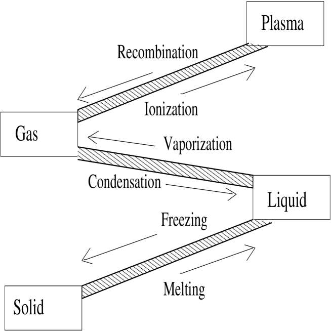
Figure 3: Classical phases and phase transitions

In the figure above, the “Recombination” transition is from a plasma to a gas. For the QCD Cosmological phases from a transition, discussed later in this section, as the Temperature of the universe dropped the matter went from a Quark-Gluon Plasma to our present universe of protons and neutrons, which is a gas (neither solid nor liquid), and later formed atomic nuclei during the first 10-100s (see Fig. 4 on Evolution of the Universe below).

As we discuss in later sections, a major project of high energy nuclear physics is to form the Quark-Gluon Plasma via the collisions of atomic nuclei such as Copper (CU), lead (Pb), and gold (Au), and to detect it by studying the production of heavy quark states.

Next we briefly describe the evolution of the universe.

The universe has evolved for about 13.7 billion years. It has gone from a very dense universe with very high temperature to our present universe, with a number of important cosmoligacal events, as illlustrated in Fig 4.

Figure 4: Evolution of the Universe

Inflation and Dark energy, which we do not discuss, occured at about $10^{-34}$ seconds. The Electroweak Phase Transition (EWPT) occured at at a time about $10^{-11}$ seconds after the big bang when the temperature (a form of energy, so we use energy units) was T $\simeq$ 125 GeV, the mass of the Higgs particle (discussed below). During the EWPT it is beleived that all particles except the photon got their mass. The QCD Phase Transition (QCDPT), the main topic in this review, occured at $t\simeq 10^{-5}$ s, with $T\simeq$ 150 MeV.

The main event that we discuss in this review is the QCDPT. Over three decades ago QCD and possible phase transitions at high T and density were discussed[5]. Inflation, the EWPT, CMBR (Cosmological Microwave Background Radiation (from which the amount of Standard and Dark Mass and Dark Energy have been measured) and events that occured after the QCDPT are discussed in detail in a recently published book[6].

3.1 Classical Phase Transitions and Latent Heat

During a first order phase transition, with a critical temperature $T_{c}$, as one adds heat the temperature stays at $T=T_{c}$ until all the matter has changes to the new phase. The heat energy that is added is called latent heat. This is illustrated in Fig 5.

In contrast to a first order phase transition, a crossover transition is a transition form one phase to another over a renge of temperatures, with no critical temperature or latent heat.

Figure 5: First order and crossover phase transitions

For application to cosmology we are mainly interested in first order phase transitions. These phase transitions occur at a critical temperature, $T_{c}$, and the temperature stays the same until all matter in the system changes to the new phase. For example if one heats water (a liquid) at standard atmospheric pressure it starts to boil, with bubbles of steam (a gas), and the temperature stays at 100 $C^{o}$. The heat energy that turns water to steam is called LATENT HEAT. This illustrated in Figure 5 above.

A familiar example of first order phase transitions is ice, a solid, melting to form water, a liquid; and water boiling to form steam, a gas. Figure 6 shows these two first order phase trasitiions for one gallon of water. Note that the latent heat for ice-water and water-steam (water vapor) is given in calories. Recognizing that heat is a form of energy, in our discussion of cosmological phase transitions we use units of energy for ther latent heat.

Figure 6: Latent heat for ice to water and water to steam

3.2 Quantum Phase Transitions

3.2.1 Brief Review of Quantum Theory

In quantum theory one does not deal with physical matter, but with states and operators. A quantum phase transition is the transition from one state to a different state. For the study of Cosmological Phase Transitions a state is the state of the universe at a particular time and temperature.

We now review some basic aspects of quantum mechanics needed for quantum phase transitions. A quantum state represents the system, and a quantum operator operates on a state. For instance, a system is in state [1] and there is an operator $A$.

$$|[1]> \equiv {\rm state[1]}$$

$$A \equiv {\rm operator\;A}\;.$$ (5)

An operator operating on a quantum state produces another quantum state. For example, operator $A$ operates on state [1]

$$A|[1]> = |[2]>\;,$$ (6)

where state [2]=$|[2]>$ is a quantum state.

State [2] might also be the same as state [1], with $|[1]>=|[2]>\equiv|A>$, except for normalization,

$$A|A> = a|A>\;,$$ (7)

where $a$ is called the eigenvalue of the operstor $A$ in state $|A>$. It is the exact value of $A$. If a state is not an eigenstate of an operator, the operator does not have an exact value.

In general, if a system is in a quantum state, the value of an operator is given by the expectation valus. For example, consider state $|[1]>$ and operator $A$.

$$<[1]| \equiv {\rm adjoint\;of\;state[1]}$$

$$<[1]|A|[1]> \equiv {\rm expectation\;value\;of\;A}\;.$$ (8)

For example, classically an electron has momentum $\vec{p}$. In quantum theory the system is in a state $|e,\vec{p}>$. The momentum operator when operating on $|e,\vec{p}>$:

$$\vec{p}_{op}|e,\vec{p}> = \vec{p}|e,\vec{p}>\;,$$ (9)

since $|e,\vec{p}>$ is an eigenstate of the operator $\vec{p}$.

In quantum theory both position $\vec{r}$ and momentum $\vec{p}$ are operators, with $p_{x}=(\not h/i)(d/dx)$, where $\not h=h/(2\pi)$ with $h$ Planks constant. Since $p_{x}x\neq xp_{x}$, a state cannot be an eigenstate of both position and momentum. If the uncertainties in x,$p_{x}$ is $\Delta x,\Delta p_{x}$ satisfy

$$\Delta p_{x}\Delta x \geq \not h/2\;,$$ (10)

which is the Heisenberg Uncertainty Principle.

3.2.2 Cosmological Phase Transitions

Calling $|0,T>$ the state of the universe at time t when it has temperature $T$, an operator $A$ has the expectation value $<0,T|A|0,T>$, as discussed above. If there is a cosmological first order phase transition, then there is a critical temperature $T_{c}$ and

$$<0,T|A|0,T>_{T<T_{c}}-<0,T|A|0,T>_{T>T_{C}} = \Delta A\;,$$ (11)

with $\Delta A$ the latent heat of the cosmological phase transitions. The two very important cosmological phase transitions are the Electroweak and QCD.

The Electroweak Phase Transition (EWPT) took place at a time $t\simeq 10^{-11}$ seconds after the Big Bang, when the critical temperature was $kT_{c}\simeq 125GeV$. The operator A in Eq(11 is the Higgs field $\Phi$. $<0,T|\Phi|0,T>_{T>T_{C}}=0$, so the latent heat for the EWPT is

$$<0,T|\Phi|0,T>_{T<T_{c}} \propto 125GeV\simeq M_{H}\;,$$ (12)

with the Higgs particle recently detected at the LHC at CERN, with the mass $M_{H}\simeq$ 125 GeV measured by the CMS[7] and ATLAS[8] collaborations. During the EWPT all standard model particles got their masses. With an additional scalar field in the standard model, usually called the Stop, the EWPT is first order, with baryogenesis (the creation of more quarks than antiquarks).

The QCD Phase Transition (QCDPT), which is the main topic in this review, took place at $t\simeq 10^{-5}$ seconds after the Big Bang, when the critical temperature was $kT^{QCDPT}_{c}\simeq 150MeV$. It is a first order phase transition and bubbles of our present universe with protons, neutrons, etc (hadrons) nucleated within the universe with a dense plasma of quarks and gluons, the Quark-Gluon Plasma (QGP) that existed when the temperature of the universe was greater than $T^{QCDPT}_{c}$. This is illustrated in Fig. 7 We shall discuss the possible detection of the QGP via heavy ion collisions.

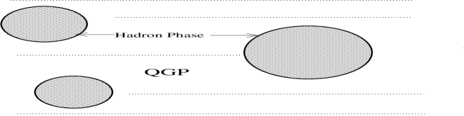
Figure 7: Hadron phase forming within the QGP during the QCDPT

3.3 The QCDPT and Quark Condensate

As reviewed above, the QCD fermion fields and particles are quarks. The Latent Heat for the QCD Phase Transition (QCDPT) is the Quark Condensate, which we now define.

$$q(x) = {\rm\;quark\;field}$$

$$\bar{q}(x) = {\rm\;antiquark\;field}$$

$$|0,T> = {\rm\;vacuum\;state\;temperature=T}$$

$$<0,T|\bar{q}(x)q(x)|0,T> = {\rm\;quark\;condensate}$$

$$= {\rm\;vacuum\;expectation\;value\;of\;\bar{q}(x)q(x)}$$

$$<0,T|\bar{q}(x)q(x)|0,T> = 0{\rm\;in\;quark\;gluon\;plasma\;phase\;T>T^{QCDPT}_{c}}$$

$$\simeq -(.23\;GeV)^{3}{\rm\;in\;hadron\;phase\;T<T^{QCDPT}_{c}}$$

The QCDPT is first order, with a discontinuity on the quark condensate at critical temperature. In Fig. 8 the results of a recent lattice gauge calculation for $<\bar{q}q>$, the quark condensate, are shown.

Figure 8: The quark condensate as a function of T=temperature

As one can see from the figure, the quark condensate $<\bar{q}q>$ goes from 0 to $(.23)^{3}GeV^{3}$ at the critical temperature of about 150 MeV, and is therefore a first order phase transition.

Although we do not discuss Dark Energy in this review, note that Dark Energy is cosmological vacuum energy, as is the quark condensate. It has been shown that Dark Energy at the present time might have been created during the QCDPT via the quark condensate[9].

4 Review of mixed hybrid heavy quark meson states

The Charmonium and Upsilon (nS) states which are important for this review are shown in Fig. 9.

Figure 9: Lowest energy Charmonium and Upsilon states

4.1 Heavy quark meson decay puzzles

Note that the standard model of the $\psi^{\prime}(2S)$ and $\Upsilon(3S)$ as $c\bar{c}$ and $b\bar{b}$ mesons is not consistent with the following puzzles:

1) The ratio of branching rarios for $c\bar{c}$ decays into hadrons (h) given by the ratios (the wave functions at the origin canceling)

$$R = \frac{B(\Psi^{\prime}(c\bar{c})\rightarrow h)}{B(J/\Psi(c\bar{c})\rightarrow h)}\;=\;\frac{B(\Psi^{\prime}(c\bar{c})\rightarrow e^{+}e^{-})}{B(J/\Psi(c\bar{c})\rightarrow e^{+}e^{-})}\simeq 0.12\;,$$

the famous 12% RULE.

The $\rho-\pi$ puzzle: The $\Psi^{\prime}(2S)$ to $J/\Psi$ ratios for $\rho-\pi$ and other h decays are more than an order of magnitude too small. Many theorists have tried and failed to explain this puzzle.

2) The Sigma Decays of Upsilon States puzzle: The $\sigma$ is a broad 600 MeV $\pi-\pi$ resonance.

$\Upsilon(2S)\rightarrow\Upsilon(1S)+2\pi$ large branching ratio. No $\sigma$

$\Upsilon(3S)\rightarrow\Upsilon(1S)+2\pi$ large branching ratio to $\sigma$

We call this the Vogel $\Delta n=2$ Rule[10]. Neither of these puzzles can be solved using standard QCD models. They were solved using the mixed heavy hybrid theory.

4.2 Hybrid, mixed heavy quark hybrid mesons, and the puzzles

The method of QCD Sum Rules[11] was used to study the heavy quark Charmonium and Upsilon states, and show that two of them are mixed hybrid meson states[12], which we now review.

4.2.1 Method of QCD Sum Rules

The starting point of the method of QCD sum rules[11] for finding the mass of a state A is the correlator,

$$\Pi^{A}(x) = \langle|T[J_{A}(x)J_{A}(0)]|\rangle\;,$$ (13)

with $|\rangle$ the vacuum state and the current $J_{A}(x)$ creating the states with quantum numbers A:

$$J_{A}(x)|\rangle = c_{A}|A\rangle+\sum_{n}c_{n}|n;A\rangle\;,$$ (14)

where $|A\rangle$ is the lowest energy state with quantum numbers A, and the states $|n;A\rangle$ are higher energy states with the A quantum numbers, which we refer to as the continuum.

The QCD sum rule is obtained by evaluating $\Pi^{A}$ in two ways. First, after a Fourier transform to momentum space, a dispersion relation gives the left-hand side (lhs) of the sum rule:

$$\Pi(q)^{A}_{\rm{lhs}} = \frac{\rm{Im}\Pi^{A}(M_{A})}{\pi(M_{A}^{2}-q^{2})}+\int_{s_{o}}^{\infty}ds\frac{\rm{Im}\Pi^{A}(s)}{\pi(s-q^{2})}$$ (15)

where $M_{A}$ is the mass of the state $A$ (assuming zero width) and $s_{o}$ is the start of the continuum–a parameter to be determined. The imaginary part of $\Pi^{A}(s)$, with the term for the state we are seeking shown as a pole (corresponding to a $\delta(s-M_{A}^{2})$ term in $\rm{Im}\Pi$), and the higher-lying states produced by $J_{A}$ known as the continuum Next $\Pi^{A}(q)$ is evaluated by an operator product expansion (O.P.E.), giving the right-hand side (rhs) of the sum rule

$$\Pi(q)_{\rm{rhs}}^{A} = \sum_{k}c_{k}(q)\langle 0|{\cal O}_{k}|0\rangle\;,$$ (16)

where $c_{k}(q)$ are the Wilson coefficients and $\langle 0|{\cal O}_{k}|0\rangle$ are gauge invariant operators constructed from quark and gluon fields, with increasing $k$ corresponding to increasing dimension of ${\cal O}_{k}$.

After a Borel transform, ${\mathcal{B}}$, in which the q variable is replaced by the Borel mass, $M_{B}$ (see Ref[11]), the final QCD sum rule, ${\mathcal{B}}\Pi_{A}(q)(LHS)={\mathcal{B}}\Pi_{A}(q)(RHS)$, has the form

$$\frac{1}{\pi}e^{-M_{A}^{2}/M_{B}^{2}}+{\cal B}\int_{s_{o}}^{\infty}\frac{Im[\Pi_{A}(s)]}{\pi(s-q^{2})}ds$$ (17)

$$= {\cal B}\sum_{k}c_{k}^{A}(q)<0|{\cal O}_{k}|0>\;.$$

This sum rule and tricks are used to find $M_{A}$, which should vary little with $M_{B}$. A gap between $M_{A}^{2}$ and $s_{o}$ is needed for accuracy. If the gap is too large, the solution is unphysical.

4.3 Mixed charmonium-Hybrid charmonium States

Recognizing that there is strong mixing between a heavy quark meson and a hybrid heavy quark meson with the same quantum numbers (defined below), the following mixed vector ($J^{PC}=1^{--}$) charmonium, hybrid charmonium current was used in QCD Sum Rules

$$J^{\mu} = bJ_{H}^{\mu}+\sqrt{1-b^{2}}J_{HH}^{\mu}$$ (18)

with

$$J_{H}^{\mu} = \bar{q}_{c}^{a}\gamma^{\mu}q_{c}^{a}$$

$$J^{\mu}_{HH} = \bar{\Psi}\Gamma_{\nu}G^{\mu\nu}\Psi\;,$$ (19)

where $\Psi$ is the heavy quark field, $\Gamma_{\nu}=C\gamma_{\nu}$, $\gamma_{\nu}$ is the usual Dirac matrix, C is the charge conjugation operator, and the gluon color field is

$$G^{\mu\nu} = \sum_{a=1}^{8}\frac{\lambda_{a}}{2}G_{a}^{\mu\nu}\;,$$ (20)

with $\lambda_{a}$ the SU(3) generator ($Tr[\lambda_{a}\lambda_{b}]=2\delta_{ab}$), discussed above.

Therefore the correlator for the mixed state:

$$\Pi_{H-HH}^{\mu\nu}(x) = <0|T[J^{\mu}(x)J^{\nu}(0)]|0>$$ (21)

is

$$\Pi_{H-HH}^{\mu\nu}(x) = b^{2}\Pi_{H}^{\mu\nu}(x)+(1-b^{2})\Pi_{HH}^{\mu\nu}(x)$$ (22)

$$+2b\sqrt{1-b^{2}}\Pi_{HHH}^{\mu\nu}(x)$$

$$\Pi_{H}^{\mu\nu}(x) = <0|T[J_{H}^{\mu}(x)J_{H}^{\nu}(0)]|0>$$

$$\Pi_{HH}^{\mu\nu}(x) = <0|T[J_{HH}^{\mu}(x)J_{HH}^{\nu}(0)]|0>$$

$$\Pi_{HHH}^{\mu\nu}(x) = <0|T[J_{H}^{\mu}(x)J_{HH}^{\nu}(0)]|0>\;,$$

where $\Pi_{H}^{\mu\nu}(x)$ is the correlator for the standard $c\bar{c}$ charm meson, $\Pi_{HH}^{\mu\nu}(x)$ is the correlator for a hybrid charm meson, with a valence gluon, and $\Pi_{HHH}^{\mu\nu}(x)$ is the correlator for a charm meson-hybrid charm meson.

It was necessary to carry out many QCD sum rule calculations to determine the value of the parameter $b$, which gives the relative probability of a normal to a hybrid meson.

The leading diagrams for the meson and meson-hybrid meson diagrams are shown in Fig. 10.

Figure 10: (a) lowest order diagram for a heavy meson (b) lowest order diagram for a meson-hybrid meson

After a Fourier transform to find the correlator in momentum space, $\Pi_{H-HH}^{\mu\nu}(p)$, the standard procedure for QCD sum rules was carried out.

Finally the Borel transform of $\Pi_{H-HH}^{\mu\nu}(p)$ was found, from which the square of the mixed meson-hybrid meson mass as function of the Borel mass, $M^{2}_{H-HH}$ was found. The result is $M^{2}_{C-HC}\simeq 3.69$ GeV=energy of the $\Psi^{\prime}(2S)$ state. A similar QCD sum rule calculation bottom heavy quarks found that the mixed upsilon-hybrid upsilon mass is $M^{2}_{\Upsilon-H\Upsilon}\simeq 10.4$ GeV= energy of the $\Upsilon(3S)$ state.

From this we conclude that the $\Psi^{\prime}(2S)$ and $\Upsilon(3S)$ states are mixed meson-hybrid meson states. This is very important for the study heavy quark state production via proton-proton collisions and RHIC for the detection of the Quark-Gluon Plasma, since a hybrid mesons have a valence gluons, as does the QGP.

For the mixed Charmonium-hybrid charmonium mass, $M^{2}_{C-HC}$, the result of the QCD sum rule analysis is shown in Fig. 11 for $b^{2}=0.5$.

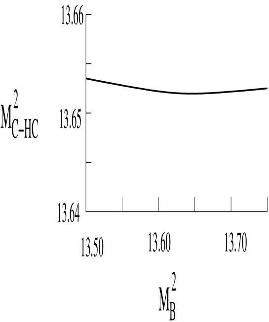
Figure 11: Mixed Charmonium-hybrid charmonium mass $\simeq$ 3.69 GeV

From this figure one sees that the minimum in $M^{2}_{C-HC}(M_{B}^{2})$ corresponds to the $\Psi^{\prime}(2S)$ state being 50% normal and 50% hybrid. The analysis for upsilon states was similar, with the $\Upsilon(3S)$ being 50% normal and 50% hybrid.

5 Heavy Quark State Production In p-p Collisions

There has been a great deal of interest in the production and polarization of heavy quark states in proton-proton collisions. In additition to the puzzles discussed above, the $J/\Psi,\Psi^{\prime}$ production anomaly[13], in which the charmonium production rate was larger than predicted for $J/\Psi$, and much larger for $\Psi^{\prime}$ than theoretical predictions in proton-proton (p-p) collisions has motivated p-p heavy quark state production experiment. In addition to being an important study of QCD, these experiments also could provide the basis for testing the production of Quark-Gluon Plasma (QGP) via a Relativistic Heavy Ion Collider (RHIC).

At the proton-proton (p-p) energies of the Fermilab, BNL-RHIC, or the Large Hadron Collider (LHC) the color octet dominates the color singlet model, which we now review.

5.1 Color Octet vs Color Singlet Heavy Quark State Production

The color octet model was shown to dominate the color singlet model[14, 15, 16]. We now discuss the Cho/Leibovich study[14, 17] which compared color octet to color singlet production. For the color singlet production they used the standard results of Ref[18] and others with $\alpha_{s}=g^{2}/(4\pi)$, where $g$ is the strong coupling constant $M=2M_{Q}$ and $q^{0}=\vec{q}^{2}/M$, with $\vec{q}$ the colliding particles momentum:

$$\sigma(gg\rightarrow Q\bar{Q}[^{1}S^{(1)}_{0}]) = \frac{\alpha^{2}_{s}M}{384\pi^{2}q^{0}s}\delta(1-M^{2}/s)\;,$$ (23)

The two color octet diagrams are shown in Fig. 12, with (a) representing quark-antiquark $\rightarrow$ gluon $\rightarrow$ color 8 quark-antiquark state $\Psi_{Q}$; and (b) reprenting gluon-gluon $\rightarrow\Psi_{Q}$.

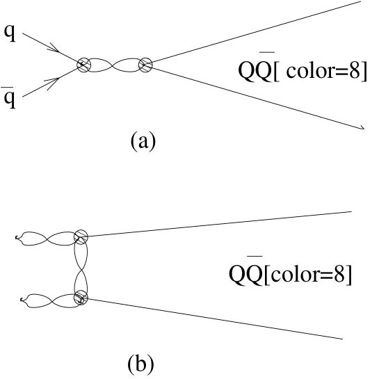
Figure 12: Color octet diagrams for (a) $q\bar{q}\rightarrow\Psi_{Q}$(8) and (b) $gg\rightarrow\Psi_{Q}$(8)

The results for the $p-\bar{p}\rightarrow J/\Psi$ theotetical transverse momentum differential cross section for the singlet and octet theories and CDF data[17] are shown in Fig. 13. Solid curve is color octet and dashed curve is color singlet production.

From this figure and references given above one sees that the color octet theory dominates. As we shall see when discussing the theory of production cross sections, there are a number of parameters that must be determined, and the diagrams shown in the figure above are not simple Feynman diagrams from which one derives the matrix elements needed to predict the cross sections.

This rather complicated theory which we discuss in the next subsection is used for p-p production of heavy quark states, which we discuss in the next subsection. It is also used in RHIC, AA production of heavy quark states, as is iscussed in the following section.

Transverse momentum diffenrential cross section for $p-\bar{p}\rightarrow J/\Psi$:

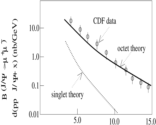
Figure 13: d$\sigma$(pp$\rightarrow$J/$\Psi$)

5.2 Proton-Proton Collisions and Production of $\Psi$ and $\Upsilon$ States

In this subsection we review the publication of Ref[19] on heavy quark state production in p-p collisions. We only consider unpolarized p-p collisions. The production cross sections are obtained from

$$\sigma_{pp\rightarrow\Phi(\lambda)} = \int_{a}^{1}\frac{dx}{x}f_{q}(x,2m)f_{\bar{q}}(a/x,2m)\sigma_{q\bar{q}\rightarrow\Phi(\lambda)}$$ (24)

$$+f_{g}(x,2m)f_{g}(a/x,2m)\sigma_{gg\rightarrow\Phi(\lambda)}\;,$$

where $a=4m^{2}/s$, with $m=1.5$ GeV for charmonium, and 5 GeV for bottomonium. $f_{g}(x,2m)$, $f_{q}(x,2m)$ are the gluonic and quark distribution functions evaluated at $Q=2m$.

For the quark and gluon cross sections, $\sigma_{q\bar{q}\rightarrow\Phi(\lambda)}$ and $\sigma_{gg\rightarrow\Phi(\lambda)}$ one needs the octet matrix elements derived from the diagrams shown in Fig.10 by Braaten and Chen[15]. The procedure of Nyyak and Smith[20] was followed in Ref[19]. The three octet matrix elements needed are $<O_{8}^{\Phi}(^{1}S_{0})>$, $<O_{8}^{\Phi}(^{3}S_{1})>$, and $<O_{8}^{\Phi}(^{3}P_{0})>$, with $\Phi$ either $J/\Psi$, $\Psi^{\prime}(2S)$, or $\Upsilon(nS)$. Since these matrix elements are not well known, Nyyak and Smith[20] use three scenerios:

$$1)<O_{8}^{\Phi}(^{1}S_{0})> = <O_{8}^{\Phi}(^{3}P_{0})>/m^{2}=.0087,$$

$$2)<O_{8}^{\Phi}(^{1}S_{0})> = .039{\rm\;and\;}<O_{8}^{\Phi}(^{3}P_{0})>=0,$$ (25)

$$3)<O_{8}^{\Phi}(^{1}S_{0})> = 0\;,$$ (26)

and $<O_{8}^{\Phi}(^{3}P_{0})>/m^{2}$=.01125, with $<O_{8}^{\Phi}(^{3}S_{1})>$=.0112 in all scenerios. All matrix elements have units GeV³. Note that these matrix elements are not used to obtain the wave functions of the heavy quark meson states.

Using[20] scenerio 2 the production cross sections[15, 20] for $\Phi$ for helicity $\lambda$ = 0 and 1 are

$$\sigma_{pp\rightarrow\Phi(\lambda=0)} = A_{\Phi}\int_{a}^{1}\frac{dx}{x}f_{g}(x,2m)f_{g}(a/x,2m)$$

$$\sigma_{pp\rightarrow\Phi(\lambda=1)} = A_{\Phi}\int_{a}^{1}\frac{dx}{x}[f_{g}(x,2m)f_{g}(a/x,2m)+0.613((f_{d}(x,2m)f_{\bar{d}}(a/x,2m)$$ (27)

$$+f_{u}(x,2m)f_{\bar{u}}(a/x,2m))]\;,$$

with $A_{\Phi}=\frac{5\pi^{3}\alpha_{s}^{2}}{288m^{3}s}<O_{8}^{\Phi}(^{1}S_{0})>$.

The main purpose of this work was to explore the effects of matrix elements for $\Psi^{\prime}(2S)$ and $\Upsilon(3S)$, comparing results with the hybrid model to the standard model. In the standard model the states are (nS) quark anti-quark states, and the ratios of the matrix elements for n greater than 1 is given by the squares of the wave functions. Note that the basis for the octet model being used is the nonrelatavistic QCD model[14, 15, 16], with a model potential for the quark anti-quark interaction giving bound states. A harmonic oscillator potential can be used to approximately give the energies of the first few states, which is what is needed in the present work. For the octet matrix elements the results of Refs.[14, 15, 16, 20] were used, as discussed above.

To approximate the ratios of matrix elements in a nonrelativistic quark model for these heavy quark meson states harmonic oscillator wave functions were used[21], with $\Phi(1S)=2Exp[-r/a_{o}]/a_{o}^{3/2}$, $\Phi(2S)=\Phi(1S)(1-r/a_{0})/2^{3/2}$, $\Phi(3S)=\Phi(1S)(1-2r/3a_{o}+2r^{2}/27a_{o}^{2})/3^{3/2}$. Defining N1= $\int|\Phi(2S)|^{2}$ divided by $\int|\Phi(1S)|^{2}$ for the 2S to 1S probability, and simillarly N2 for the 3S to 1S probability, we find N1=0.039, N2=0.0064, N3=N2/N1=.16. This is a very rough estimate. Therefore, we use $A_{\Psi^{\prime}(2S)}=0.039A_{J/\Psi(1S)}$, $A_{\Upsilon(2S)}=0.039A_{\Upsilon(1S)}$, and $A_{\Upsilon(3S)}=0.0064A_{\Upsilon(1S)}$ in the standard model.

On the other hand in the mixed hybrid study both $\Psi^{\prime}(2S)$ and $\Upsilon(3S)$ were found to be approximately 50% hybrids. In Ref[12] it was shown, using the external field method, that the octet to singlet matrix element was enhanced by a factor of $\pi^{2}$ compared to the standard model, as illustrated in Fig.14. For mixed hybrids an enhancement factor of 3.0 was used.

Figure 14: External field method for $\Psi^{\prime}(2S)$ and $\Upsilon(3S)$ states

For differential cross sections the rapidity variable, $y$, is used,

$$y(x) = \frac{1}{2}ln(\frac{E+p_{z}}{E-p_{z}}){\rm;\;with\;}E=\sqrt{M^{2}+p_{z}^{2}}$$

$$p_{z} = \frac{\sqrt{s}}{2}(x-\frac{a}{x})\;,$$ (28)

or

$$x(y) = 0.5\left[\frac{m}{s}(\exp{y}-\exp{(-y)})+\sqrt{(\frac{m}{s}(\exp{y}-\exp{(-y)}))^{2}+4a}\right]$$ (29)

For the unpolarized proton collisions we use a polynomial fit to the parton distributions of Ref.[22]. Because of the wide range of vaues, in order to obtain a good polynomial fit to the parton distributions we limit the range of rapidity to $-1.<y<1.$

For Q=3 GeV, with m=Charmonium mass = 1.5 GeV, from Eq(29), x has a range about 0.028 to 0.032, and a/x 0.008 to 0.015. In Ref[19] the following expressions were derived for the gluon (g), u and d quark, and anti-quark distribution functions using QTEQ6 for Q=3 GeV, fitting the range x=0.008 to .004, which is needed for $\sqrt{s}\simeq$ 200 to 500 GeV

$$f_{g}(x) \simeq 1334.21-67056.5x+887962.0x^{2}$$

$$f_{d}(x) \simeq 72.956-3281.1x+42247.6x^{2}$$

$$f_{u}(x) \simeq 82.33-3582.36x+45867.3x^{2}$$

$$f_{\bar{u}}(x) \simeq 55.98-2722.04x+35641.2x^{2}$$ (30)

$$f_{\bar{d}}(x) \simeq 57.44-2757.05x+36030.5x^{2}\;.$$

For Q=10 GeV, m=Bottomonium mass=5 GeV, from Eq(29), x has a range about 0.05 to 0.08, and a/x 0.03 to 0.05. We have derived the following expressions for the gluon (g), u and d quark, and antiquark distribution functions using QTEQ6 for Q=10 GeV, fitting the range x=0.03 to .08, which is needed for $\sqrt{s}$=38.8 GeV and 2.76 TeV.

$$f_{g}(x) \simeq 275.14-6167.6x+36871.3x^{2}$$

$$f_{d}(x) \simeq 26.96-527.14x+3119.13x^{2}$$

$$f_{u}(x) \simeq 32.92-604.38x+3530.1x^{2}$$

$$f_{\bar{u}}(x) \simeq 16.64-377.53x+2336.86x^{2}$$ (31)

$$f_{\bar{d}}(x) \simeq 17.81-390.64x+2392.46x^{2}\;.$$

The differential rapidity distribution for $\lambda=0$ is given by

$$\frac{d\sigma_{pp\rightarrow\Phi(\lambda=0)}}{dy} = A_{\Phi}\frac{1}{x(y)}f_{g}(x(y),2m)f_{g}(a/x(y),2m)\frac{dx}{dy}\;,$$ (32)

while for $\lambda$=1

$$\frac{d\sigma_{pp\rightarrow\Phi(\lambda=1)}}{dy} = A_{\Phi}\frac{1}{x(y)}[f_{g}(x(y),2m)f_{g}(a/x(y),2m)+0.613(f_{d}(x(y),2m)f_{\bar{d}}(a/x(y),2m)$$ (33)

$$+f_{u}(x(y),2m)f_{\bar{u}}(a/x(y),2m)]\frac{dx}{dy}\;.$$

5.2.1 Charmonium Production Via Unpolarized p-p Collisions at E=$\sqrt{s}$= 200 GeV at BNL-RHIC

Unpolarized p-p collisions for $\sqrt{s}=200GeV$ corresponding to BNL energy, using scenerio, with the nonperturbative matrix elements given above, $A_{\Phi}=\frac{5\pi^{3}\alpha_{s}^{2}}{288m^{3}s}<O_{8}^{\Phi}(^{1}S_{0})>$ =$7.9\times 10^{-4}$nb for $\Phi$=$J/\Psi$ and $2.13\times 10^{-5}$nb for $\Upsilon(1S)$ heavy quark states.

For $\sqrt{s}=200GeV$

$$x(y) = 0.5\left[\frac{m}{200}(\exp{y}-\exp{(-y)})+\sqrt{(\frac{m}{200}(\exp{y}-\exp{(-y)}))^{2}+4a}\right]$$

$$\frac{dx(y)}{dy} = \frac{M}{400}(\exp{y}+\exp{(-y)})\left[1.+\frac{\frac{M}{200}(\exp{y}-\exp{(-y)})}{\sqrt{(\frac{M}{200}(\exp{y}-\exp{(-y)}))^{2}+4a}}\right]\;.$$ (34)

Note that there was a typo error in Ref[19], with $\frac{M}{200}(\exp{y}+\exp{(-y)})$ instead of $\frac{M}{200}(\exp{y}-\exp{(-y)})$ in the numerator of Eq(5.2.1). Using Eqs(32,33,5.2.1), with the parton distribution functions given in Eq(5.2), we find d$\sigma$/dy for Q=3 GeV, $\lambda=0$ and $\lambda=1$ the results for $J/\Psi$ shown in Figure 15.

Figure 15: d$\sigma$/dy for Q=3 GeV, E=200 GeV unpolarized p-p collisions producing $J/\Psi$ with $\lambda=0$, $\lambda=1$

Note that the shape of d$\sigma$/dy is consistent with the BNL-RHIC-PHENIX detector rapidity distribution[23].

For $\Psi^{\prime}(2S)$ the results are shown in Figure 16 for both the standard model and the mixed hybrid theory.

Figure 16: d$\sigma$/dy for Q= 3 GeV, E=200 GeV unpolarized p-p collisions producing$\Psi^{\prime}(2S)$ with $\lambda=1$,$\lambda=0$

The results for d$\sigma$/dy shown in Figure 16 labeled $\Psi^{\prime}(2S)(a)$ are obtained by using for the standard nonperturbative matrix element=0.039 times the matrix elements for $J/\Psi$ production; while the results labeled $\Psi^{\prime}(2S)(b)$ are obtained by using the matrix element derived using the result that the $\Psi^{\prime}(2S)$ is approximately 50% a hybrid with the enhancement is at least a factor of $\pi$, as discussed above.

5.2.2 Upsilon Production Via Unpolarized p-p Collisions at E=$\sqrt{s}$= 38.8 GeV at Fermilab

In this subsection the cross sections calculated for for $\Upsilon(nS)$ production, with n= 1, 2, 3 at 38.8, which has been measured at Fermilab[24, 25], are reviewed.

For Q=10 GeV, using the parton distributions given in Eq(5.2) and Eqs(32,33) for helicity $\lambda=0$, $\lambda=1$, with $A_{\Upsilon}$ =$5.66\times 10^{-4}$nb and $a=6.64\times 10^{-2}$, one obtains $d\sigma/dy$ for $\Upsilon(nS)$ production.

The results for $\Upsilon(1S)$, $\Upsilon(2S)$ are shown in Figure 17, and for $\Upsilon(3S)$ in Figure 18.

Figure 17: d$\sigma$/dy for Q= 10 GeV, E=38.8 GeV unpolarized p-p collisions producing $\Upsilon(1S)$, $\Upsilon(2S)$ with $\lambda=0$, $\lambda=1$

Figure 18: d$\sigma$/dy for Q= 10 GeV, E=38.8 GeV unpolarized p-p collisions producing $\Upsilon(3S)$ with $\lambda=0$, $\lambda=1$. Results labeled a,b are for the standard, mixed hybrid theories.

It should be noted that the ratios of $d\sigma/dy$ for $\Psi^{\prime}(2S)$/$J/\Psi$, and $\Upsilon(3S)$/($\Upsilon(1S)$+$\Upsilon(2S)$) for the hybrid theory vs. the standard are our most significant results, as there are uncertainties in the absolute magnitudes and shapes of $d\sigma/dy$ on the scenerios, as well as the magnitudes of the matrix elements.

5.2.3 Polarized p-p collisions for E=200 GeV at BNL-RHIC

For polarized p-p collisions the equations for $\frac{d\sigma_{pp\rightarrow\Phi(\lambda=0)}}{dy}$ and $\frac{d\sigma_{pp\rightarrow\Phi(\lambda=1)}}{dy}$ are the same as Eqs(32,33) with the parton distribution functions $fg$ and $fq$ given in Eqs(5.2,5.2) replaced by $\Delta fg$ and $\Delta fq$, the parton distribution functions for longitudinally polarized p-p collisions. A fit to the parton distribution functions for polarized p-p collisions for Q=3 GeV obtained from CTEQ6[22] in the x range needed for $\sqrt{s}$=200 GeV is

$$\Delta f_{g}(x) \simeq 15.99-700.34x+13885.4x^{2}-97888.x^{3}$$

$$\Delta f_{d}(x) \simeq -5.378.+205.60x-4032.77x^{2}+28371.x^{3}$$

$$\Delta f_{u}(x) \simeq 8.44-292.19x+5675.16x^{2}-39722.x^{3}$$

$$\Delta f_{\bar{u}}(x) \simeq -1.447+64.67x-1268.24x^{2}+8878.32x^{3}$$ (35)

$$\Delta f_{\bar{d}}(x) = \Delta f_{\bar{u}}(x)\;,$$

and for Q=10 GeV, which we do not use in the present work, as the $\Upsilon(nS)$ are not resolved at BNL-RHIC,

$$\Delta f_{g}10(x) \simeq 28.98-1435.47x+29533.5x^{2}-211440.x^{3}$$

$$\Delta f_{d}10(x) \simeq -6.074+241.57x-4762.04x^{2}+33604.4x^{3}$$

$$\Delta f_{u}10(x) \simeq 9.88-348.632x+6729.49x^{2}-47058.x^{3}$$

$$\Delta f_{\bar{u}}10(x) \simeq -1.552+75.731x-1531.97x^{2}+10896.6x^{3}$$ (36)

$$\Delta f_{\bar{d}}10(x) = \Delta f_{\bar{u}}10(x)\;.$$

The differential rapidity distribution for polarized p-p collisions are

$$\frac{d\Delta\sigma_{pp\rightarrow\Phi(\lambda=0)}}{dy} = -A_{\Phi}\frac{1}{x(y)}\Delta f_{g}(x(y),2m)\Delta f_{g}(a/x(y),2m)\frac{dx}{dy}\;,$$ (37)

$$\frac{d\Delta\sigma_{pp\rightarrow\Phi(\lambda=1)}}{dy} = -A_{\Phi}\frac{1}{x}[\Delta f_{g}(x(y),2m)\Delta f_{g}(a/x(y),2m)-0.613(\Delta f_{d}(x(y),2m)$$ (38)

$$\Delta f_{\bar{d}}(a/x(y),2m)+\Delta f_{u}(x(y),2m)\Delta f_{\bar{u}}(a/x(y),2m)]\frac{dx}{dy}\;.$$

For polarized p-p collisions, Q=3 GeV, the results for d$\Delta\sigma$/dy for $J/\Psi$ production using the standard model are shown in Figure 19 while for $\Psi^{\prime}(2S)$ the results are shown in Figure 20. As above, the curves labelled $\Psi^{\prime}(2S)a$ and are the standard model results, while that labelled $\Psi^{\prime}(2S)b$ are the results for a mixed hybrid. The enhancement from active glue is once more quite evident. Since $\Upsilon(nS)$ states have not been resolved at BNL-RHIC, where polarized p-p collisions were measured, we do not calculate d$\Delta\sigma$/dy for $\Upsilon(nS)$ states.

Figure 19: d$\Delta\sigma$/dy for Q=3 GeV, E=200 GeV polarized p-p collisions producing $J/\Psi$, with $\lambda=0$, $\lambda=1$

Figure 20: d$\Delta\sigma$/dy for Q= 3 GeV, E=200 GeV polarized p-p collisions producing $\Psi^{\prime}(2S)$ with $\lambda=0$, $\lambda=1$

Once again, it is the ratios of $d\Delta\sigma/dy$ that are most significant, as there is uncertainty both the absolute magnitudes and shapes.

5.2.4 Ratios of Cross Sections for $\Psi$, $\Upsilon$ Production Via p-p Collisions

Because of problems with normalization we cannot compare our cross sections directly with experiment, but a comparison of ratios of cross sections with experiment is an excellent test of the theory used to estimate $\Psi^{\prime}(2S),J/\Psi(1)$ $\Psi$ and $\Upsilon$ production.

In this subsection the cross sections for $\Psi^{\prime}(2S),J/\Psi(1)$, $\Upsilon(nS)$, production, with n= 1, 2, 3 are calculated, and then the theory that $\Psi^{\prime}(2S),\Upsilon(3S)$ are hybrids is used to estimate the ratios of cross section. Since with scenerio 2 with $<O_{8}^{\Phi}(^{3}P_{0})>$=0, the $\lambda=0$ helicity dominates the cross section[20], the $\lambda=1$ terms were dropped. From Eq(5.2), for $\lambda=0$, the cross section is determined from

$$\sigma_{pp\rightarrow\Phi(\lambda=0)} = A_{\Phi}\int_{a}^{1}\frac{dx}{x}f_{g}(x,2m)f_{g}(a/x,2m)\;,$$ (39)

where

$$A_{\Phi} \propto \frac{1}{s}\;,$$ (40)

with $s=E^{2}$, as discussed above. The energy dependence of $\sigma_{pp\rightarrow\Phi(\lambda=0)}$ of Eq(39), given by Eq(40) will be compared to experiment in the next subsection.

As discussed ref[19] the estimated ratios for p-p production of $\Psi(2S)$ and $J/\Psi(1S)$ using the harmonic-oscillator wave functions for the standard model and a factor $\simeq\pi$ for the mixed hybrid theory are

$$\sigma(\Psi(2S))/\sigma(J/\Psi(1S))|_{standard} \simeq 0.039$$

$$\sigma(\Psi(2S))/\sigma(J/\Psi(1S))|_{hybrid} \simeq 0.122\;,$$ (41)

while the estimated $\Upsilon(2S),\Upsilon(3S)$ to $\Upsilon(1S)$ ratios are

$$\sigma(\Upsilon(2S))/\sigma(\Upsilon(1S))|_{standard} \simeq \sigma(\Upsilon(2S))/\sigma(\Upsilon(1S))|_{hybrid}\simeq 0.039$$

$$\sigma(\Upsilon(3S))/\sigma(\Upsilon(1S))|_{standard} \simeq .0064$$

$$\sigma(\Upsilon(3S))/\sigma(\Upsilon(1S))|_{hybrid} \simeq 0.0201\;.$$ (42)

From the recent measurements by the ALICE Collaboration[34] the $\Psi(2S)$ to $J/\Psi(1S)$ ratio is

$$\frac{\sigma_{\Psi(2S)}}{\sigma_{J/\Psi}}\simeq 0.170\pm 0.011(stat)\pm 0.013(syst)\;,$$ (43)

one can see from Eq(43) that the $\sigma_{\Psi(2S)}/\sigma_{J/\Psi}$ ratio is much larger than the standard model and is consistent with the mixed hybrid theory[12] within theoretical and expermental errors.

The $\Upsilon(2S),\Upsilon(3S)$ to $\Upsilon(1S)$ ratios are difficult for experiments to measure. These ratios at E= 7 TeV were recently measured by the ATLAS Collaboration[35]. The ratios of cross sections include the branching fractions, $BR(\Upsilon\rightarrow\mu^{+}\mu^{-})$, with the experimental results Because of the branching fractions, it is difficult to compare the ATLAS results to the theoretical cross section ratios given in Eq(5.2.4). However, the energy dependence of $\Upsilon$ cross section can be measured, as discussed in the next subsection.

5.2.5 Theoretical vs Experimental Energy Dependence of $\Upsilon$ Cross Sections

Note that $A_{\Phi}$ from Eq(40) has the property $A_{\Phi}(s)\propto 1/s$, so cross sections should also be $\propto 1/s$. Recently, LHCb measured experimental ratios at 7 and 8 TeV at forward rapidity for $\Upsilon(1S),\Upsilon(2S),\Upsilon(3S)$ production[36]. The theoretical and the experiment ratios are

$$(\sigma_{\Upsilon}(8TeV)/\sigma_{\Upsilon}(7TeV))_{theory} \simeq 1.306$$

$$(\sigma_{\Upsilon}(8TeV)/\sigma_{\Upsilon}(7TeV))_{experiment} \simeq 1.291\pm 0.005\;,$$ (44)

so the theoretical ratio for different energies is consistent with experiment within errors.

5.2.6 Conclusions of Ref[19]

The mixed hybrid theory for heavy quark states was used to predict that the cross sections for production of the charmonium $\Psi^{\prime}(2S)$ state in 200 GeV p-p collisions and bottomonium $\Upsilon(3S)$ states in 38.8 GeV p-p collisions are much larger than the standard model. Also the estimated ratio of cross sections for 2.76 TeV and 38.8 GeV experiments, and the prediction for the $\Upsilon(3S)$ production cross section is larger than the standard model, and closer to the experimental values.

Because of the importance of gluonic production in processes in a Quark Gluon Plasma, this could lead to a test of the creation of QGP in RHIC.

5.2.7 Upsilon Production In p-p Collisions For Forward Rapidities At LHC

In the work on p-p collisions producing heavy quark states reviewed above the rapidity was y=-1 to 1, while the present study is for y=2.5 to 4.0 at the LHC[26]. The differential rapidity distribution for Upsilon production with $\lambda=0$ (dominant for $\Upsilon(nS)$ production), as is given by

$$\frac{d\sigma_{pp\rightarrow\Phi(\lambda=0)}}{dy} = A_{\Upsilon}\frac{1}{x(y)}f_{g}(x(y),2m)f_{g}(a/x(y),2m)\frac{dx}{dy}\;,$$ (45)

with $x(y),\frac{dx(y)}{dy}$ defined in Eq(5.2.1) and $A_{\Upsilon}=1.12\times 10^{-7},1.73\times 10^{-8}$ nb, for $\sqrt{s}$ = 2.76, 7.0 TeV. $f_{g}$ is the gluonic distribution function given in Eq(5.2) for the energies at the LHC.

Using Eqs(45,5.2) and parameters given in Ref[19] we obtain the results for $\Upsilon(1S)$ and $\Upsilon(3S)$ production shown in Fig. 21 and Fig. 22 at 2.76 TeV and 7.0 TeV[27] in p-p collisions for $2.5\leq y\leq 4.0$. Although the units in Figs. 21, 22 are in pb, the actual magnitude is uncertain due to the normalization of the state. The overall magnitude and rapidity dependence of the differential rapidity distribution, however, provides satisfactory estimates at forward rapidities for LHC experiments.

Also, it is the ratios of cross sections, $\sigma(\Upsilon(2S))/\sigma(\Upsilon(1S))$ and $\sigma(\Upsilon(3S))/\sigma(\Upsilon(1S))$ which are most accurate, and are used to prove that the mixed hybrid theory for $\Upsilon(3S))$ is much better than the standard $b\bar{b}$ model. This is discussed in detail in the next section.

Figure 21: d$\sigma$/dy for pp collisions at $\sqrt{s}$ = 2.76 and 7.0 producing $\Upsilon(1S)$.

Figure 22: d$\sigma$/dy for pp collisions at $\sqrt{s}$ = 2.76 and 7.0 TeV producing $\Upsilon(3S)$.

5.2.8 $\Psi$ and $\Upsilon$ Production In pp Collisions at E=7.0 TeV

This is an extension of recent studies for $\Upsilon(nS)$ and $\Psi(1S,2S)$ production at the LHC in p-p collisions with E=7.0 GeV and the ALICE detector[29]. The differential rapidity cross section is the same as Eq(45) with $A_{\Upsilon}=1.73\times 10^{-8}$ nb for E= 7.0 TeV, and $A_{\Upsilon}\rightarrow A_{\Psi}=6.46\times 10^{-7}$. The gluonic distribution $f_{g}$ is the same as in Eq(5.2). The calculation of the production of $\Upsilon(3S)$ and $\Psi(2S)$ states is done with the mixed heavy hybrid theory[12].

Figure 23: d$\sigma$/dy for pp collisions at $\sqrt{s}$ = 7.0 TeV producing $\Upsilon(1S)$.

The differential rapidity cross sections for $\Upsilon(1S)$, $\Upsilon(2S)$ with the standard model are shown in Figs. 23, 24; and for $\Upsilon(3S)$ with the standard model and mixed hybrid theory are shown in Fig. 25.

Figure 24: d$\sigma$/dy for pp collisions at $\sqrt{s}$ = 7.0 TeV producing $\Upsilon(2S)$.

Figure 25: d$\sigma$/dy for pp collisions at $\sqrt{s}$ = 7.0 TeV producing $\Upsilon(3S)$ for usual and hybrid theories.

The differential rapidity cross sections for $J/\Psi(1S)$ and $\Psi(2S)$ are shown in Figures 26 and 27.

Figure 26: d$\sigma$/dy for pp collisions at $\sqrt{s}$ = 7.0 TeV producing $J/\Psi(1S)$.

Figure 27: d$\sigma$/dy for pp collisions at $\sqrt{s}$ = 7.0 TeV producing $\Psi(2S)$ for usual and hybrid theories.

For $\Upsilon(3S)$ and $\Psi(2S)$ the standard $q\bar{q}$ prediction is shown by dashed curves, while the prediction using the mixed hybrid theory[12] is shown with solid curves, with the difference explained in Ref[19].

5.2.9 $\Psi$ and $\Upsilon$ Production In p-p Collisions at E=8.0 TeV

This is an extension of the preceeding subsubsection for $\Upsilon(nS),n=1,2,3,$ and $J/\Psi(1S),\Psi(2S)$ production in p-p collisions with the ALICE detector at 7.0 TeV, with new predictions for p-p collisions at the LHC-ALICE with E=8.0 TeV[30]. The differential rapidity cross section is the same as Eq(45) with $A_{\Upsilon}=1.33\times 10^{-8}$ and $A_{\Upsilon}\rightarrow A_{\Psi}=4.95\times 10^{-7}$ for E= 8.0 TeV. The gluonic distribution $f_{g}(x(y),2m)$ for the range of $x$ needed for $E=8.0$ TeV is the same as Eq(5.2).

The calculation of the production of $\Upsilon(3S)$ and $\Psi(2S)$ states is done with the usual quark-antiquark model and the mixed heavy quark hybrid theory, as in the previous subsections.

The differential rapidity cross sections for $J/\Psi(1S)$ and $\Psi(2S)$ production for the standard model and the mixed hybrid theory are shown in Figure 28.

Figure 28: d$\sigma$/dy for p-p collisions at $\sqrt{s}$ = 8.0 TeV producing $J/\Psi(1S)$; and $\Psi(2S)$ for the standard model (dashed curve) and the mixed hybrid theory.

The differential rapidity cross sections for $\Upsilon(1S)$, $\Upsilon(2S)$, and $\Upsilon(3S)$ are shown in Figure 29.

Figure 29: d$\sigma$/dy for p-p collisions at $\sqrt{s}$ = 8.0 TeV for producing $\Upsilon(1S)$, $\Upsilon(2S)$, $\Upsilon(3S)$ (dashed curve) using the standard model; and $\Upsilon(3S)$ with the mixed hybrid theory.

5.2.10 $\Psi$ and $\Upsilon$ Production In p-p Collisions at E=13 TeV

Motivated by the LHC modification in 2015, this subsubsection is an extension of the preceeding subsubsections for p-p collisions at E=7.0, 8.0 TeV with predictions of $\Upsilon(nS),n=1,2,3,$ and $J/\Psi(1S),\Psi(2S)$ production in p-p collisions at 13 TeV[31]

The differential rapidity cross sections for $J/\Psi(1S)$ and $\Psi(2S)$ production for the standard model and the mixed hybrid theory for p-p collisions at E=13 TeV are shown in Figure 30.

Figure 30: d$\sigma$/dy for p-p collisions at $\sqrt{s}$ = 13.0 TeV producing $J/\Psi(1S)$; and $\Psi(2S)$ for the standard model (dashed curve) and the mixed hybrid theory.

Differential rapidity cross sections $\Upsilon$ production for p-p collisions at 13 TeV are shown in Figure 31.

Figure 31: d$\sigma$/dy for p-p collisions at $\sqrt{s}$ = 13.0 TeV producing $\Upsilon(1S)$, $\Upsilon(2S)$, and $\Upsilon(3S)$ for the standard model (dashed curve) and the mixed hybrid theory.

5.2.11 $\Psi$ and $\Upsilon$ Production In p-p Collisions at E=14 TeV

This subsubsection is an extension of the preceeding subsubsection for p-p collisions at E=13 TeV with predictions of $J/\Psi(1S),\Psi(2S),\Upsilon(1S),\Upsilon(2S),\Upsilon(3S)$ production via p-p collisions at 14 TeV, based on recent research [32]. Although the rapidity dependence of d$\sigma$/dy, shown in the figures for p-p collisions at 14 TeV, are similar to those at 13TeV, with the LHC energy will be increased to 14 TeV during the LHC’s second run period starting in 2015. This should be useful for comparison with experiments. The differential rapidity cross sections for $J/\Psi(1S)$ and $\Psi(2S)$ production for the standard model and the mixed hybrid theory are shown in Figure 32.

Figure 32: d$\sigma$/dy for p-p collisions at $\sqrt{s}$ = 14.0 TeV producing $J/\Psi(1S)$; and $\Psi(2S)$ for the standard model (dashed curve) and the mixed hybrid theory.

The differential rapidity cross sections for $\Upsilon(1S),\Upsilon(2S),\Upsilon(3)$ production for the standard model and the mixed hybrid theory are shown in Figure 33.

Figure 33: d$\sigma$/dy for p-p collisions at $\sqrt{s}$ = 14.0 TeV producing $\Upsilon(1S)$, $\Upsilon(2S)$, and $\Upsilon(3S)$ for the standard model (dashed curve) and the mixed hybrid theory.

6 Heavy-quark state production in A-A collisions at $\sqrt{s_{pp}}$=200 GeV

This section is a review of Ref[33]. The differential rapidity cross section for the production of a heavy quark state $\Phi$ with helicirkty $\lambda=0$ in the color octet model via A-A collisions is given by

$$\frac{d\sigma_{AA\rightarrow\Phi(\lambda=0)}}{dy} = R_{AA}N^{AA}_{bin}<\frac{d\sigma_{pp\rightarrow\Phi(\lambda=0)}}{dy}>\;,$$ (46)

where $R_{AA}$ is the nuclear modification factor, defined in Ref[38], which includes the dissociation factor after the state $\Phi$ is formed[39]. See Refs.[40],[41] for a discussion of “cold nuclear matter effects” and references to earlier experimental and theoretical publications. $N^{AA}_{bin}$ is the number of binary collisions in the A-A collision, and $<\frac{d\sigma_{pp\rightarrow\Phi(\lambda=0)}}{dy}>$ is the differential rapidity cross section for $\Phi$ production via nucleon-nucleon collisions in the nuclear medium. Note that $R^{E}_{AA}$, which we take as a constant, can be functions of rapidity. See Refs[42, 41] for a review and references to many publications.

Experimental studies show that for $\sqrt{s_{pp}}$ = 200 GeV $R_{AA}\simeq 0.5$ both for Cu-Cu[43, 44] and Au-Au[45, 46, 58]. The number of binary collisions are $N^{AA}_{bin}$=51.5 for Cu-Cu[59] and 258 for Au-Au. The differential rapidity cross section for p-p collisions in terms of $f_{g}$[22, 19], the gluon distribution function ($-0.8\leq y\leq 0.8$ for $\sqrt{s_{pp}}$ = 200 GeV with $f_{g}$ from Ref[19]), is

$$<\frac{d\sigma_{pp\rightarrow\Phi(\lambda=0)}}{dy}> = A_{\Phi}\frac{1}{\bar{x}(y)}f_{g}(\bar{x}(y),2m)f_{g}(a/\bar{x}(y),2m)\frac{dx}{dy}\;,$$ (47)

where, as is discussed above, $a=4m^{2}/s$; with $m=1.5$ GeV for charmonium, and 5 GeV for bottomonium, and $A_{\Phi}=\frac{5\pi^{3}\alpha_{s}^{2}}{288m^{3}s}<O_{8}^{\Phi}(^{1}S_{0})>$ [19]. For $\sqrt{s_{pp}}$ = 200 GeV $A_{\Phi}=7.9\times 10^{-4}$nb for $\Phi$=$J/\Psi$ and $2.13\times 10^{-5}$nb for $\Upsilon(1S)$; $a=2.25\times 10^{-4}$ for Charmonium and $2.5\times 10^{-3}$ for Bottomium.

The function $\bar{x}$, the effective parton x in a nucleus (A), is given in Refs[47, 48]:

$$\bar{x}(y) = x(y)(1+\frac{\xi_{g}^{2}(A^{1/3}-1)}{Q^{2}})$$

$$x(y) = 0.5\left[\frac{m}{\sqrt{s_{pp}}}(\exp{y}-\exp{(-y)})+\sqrt{(\frac{m}{\sqrt{s_{pp}}}(\exp{y}-\exp{(-y)}))^{2}+4a}\right]\;,$$ (48)

with[49] $\xi_{g}^{2}=.12GeV^{2}$. For $J/\Psi$ $Q^{2}=10GeV^{2}$, so $\bar{x}=1.058x$ for Au and $\bar{x}=1.036x$ for Cu, while for $\Upsilon(1S)$ $Q^{2}=100GeV^{2}$, so $\bar{x}=1.006x$ for Au and $\bar{x}=1.004x$ for Cu.

From this we find the differential rapidity cross sections as shown Figs. 34-41 for $J/\Psi,\Psi(2S)$ and $\Upsilon(1S),\Upsilon(2S),\Upsilon(3S)$ production via Cu-Cu and Au-Au collisions at RHIC (E=200 GeV), with $\Psi(2S),\Upsilon(3S)$ enhanced by $\pi^{2}/4$ as discussed above. The absolute magnitudes are uncertain, and the shapes and relative magnitudes are our main prediction.

Figure 34: d$\sigma$/dy for 2m=3 GeV, E=200 GeV Cu-Cu collisions producing $J/\Psi$ with $\lambda=0$

Figure 35: d$\sigma$/dy for 2m=3 GeV, E=200 GeV Au-Au collisions producing $J/\Psi$ with $\lambda=0$

Figure 36: d$\sigma$/dy for 2m=3 GeV, E=200 GeV Cu-Cu collisions producing $\Psi(2S)$ with $\lambda=0$. The dashed curve is for the standard $c\bar{c}$ model.

Figure 37: d$\sigma$/dy for 2m=3 GeV, E=200 GeV Au-Au collisions producing $\Psi(2S)$ with $\lambda=0$. The dashed curve is for the standard $c\bar{c}$ model.

Figure 38: d$\sigma$/dy for 2m=10 GeV, E=200 GeV Cu-Cu collisions producing $\Upsilon(1S)$ with $\lambda=0$

Figure 39: d$\sigma$/dy for 2m=10 GeV, E=200 GeV Au-Au collisions producing $\Upsilon(1S)$ with $\lambda=0$

Figure 40: d$\sigma$/dy for 2m=10 GeV, E=200 GeV Cu-Cu collisions producing $\Upsilon(2S),\Upsilon(3S)$ with $\lambda=0$. For $\Upsilon(3S)$ the dashed curve is for the standard $b\bar{b}$ model.

Figure 41: d$\sigma$/dy for 2m=10 GeV, E=200 GeV Au-Au collisions producing $\Upsilon(2S),\Upsilon(3S)$ with $\lambda=0$. For $\Upsilon(3S)$ the dashed curve is for the standard $b\bar{b}$ model.

6.1 Ratios of $\Psi^{\prime}(2S)$ to $J/\Psi$ cross sections for A-A collisions

As discussed above, for the standard (st), hybrid model(hy) one finds for p-p production of $\Psi^{\prime}(2S)$ and $J/\Psi$

$$\sigma(\Psi^{\prime}(2S))/\sigma(J/\Psi(1S))|_{st} \simeq 0.039$$

$$\sigma(\Psi^{\prime}(2S))/\sigma(J/\Psi(1S))|_{hy} \simeq 0.122\;,$$ (49)

while the PHENIX experimental result for the ratio[51] $\simeq 0.18\pm.04$. Therefore, the hybrid model is consistent with experiment, while the standard model ratio is too small.

The recent CMS/LHC result comparing Pb-Pb to p-p Upsilon production[50] found

$$[\frac{\Upsilon(2S)+\Upsilon(3S)}{\Upsilon(1S)}]_{Pb-Pb}/[\frac{\Upsilon(2S)+\Upsilon(3S)}{\Upsilon(1S)}]_{p-p} \simeq 0.31^{+.19}_{-.15}\pm.013(syst)\;,$$ (50)

while in the work discussed previously on $p-p$ collisions the ratio $\sigma(\Upsilon(3S))/\sigma(\Upsilon(1S))|_{p-p}$ of the standard $|b\bar{b}>$ model was $4/\pi^{2}\simeq 0.4$ of the hybrid model. This suggests a suppression factor for $\sigma(b\bar{b}(3S))/\sigma(b\bar{b}(1S))$, or $\sigma(c\bar{c}(2S)/\sigma(c\bar{c}(1S))$ of 0.31/.4 as these components travel through the QGP; or an additional factor of 0.78 for $\Psi^{\prime}(2S)$ to $J/\Psi$ production for $A-A$ vs $p-p$ collisions. Therefore from Eq(6.1) one obtains the estimate using the mixed hybrid theory for this ratio

$$\sigma(\Psi^{\prime}(2S))/\sigma(J/\Psi(1S))|_{A-A{\rm\;collisions}} \simeq 0.10$$ (51)

6.2 Ratios of $\Upsilon(2S)$ and $\Upsilon(3S)$ to $\Upsilon(1S)$ cross sections for Pb-Pb vs p-p collisions

As pointed out in Eq(5.2.4), $\sigma(\Upsilon(2S))/\sigma(\Upsilon(1S))|_{standard}\simeq\sigma(\Upsilon(2S))/\sigma(\Upsilon(1S))|_{hybrid}\simeq 0.039$, $\sigma(\Upsilon(3S))/\sigma(\Upsilon(1S))|_{standard}\simeq.0064$, Although the ratio $\sigma(\Upsilon(3S))/\sigma(\Upsilon(1S))$ is difficult to measure, as pointed out above, the ratios of cross sections for $\sigma(\Upsilon(2S))/\sigma(\Upsilon(1S))$ and $\sigma(\Upsilon(3S))/\sigma(\Upsilon(1S))$ for A-A vs p-p can be measured.

The recent CMS experiment’s main objective[52] is to test for $\Upsilon$ suppression in PbPb collisions, with estimates of the following quantities:

$$\frac{[\Upsilon(2S)/\Upsilon(1S)]_{PbPb}}{[\Upsilon(2S)/\Upsilon(1S)]_{pp}}$$

$$\frac{[\Upsilon(3S)/\Upsilon(1S)]_{PbPb}}{[\Upsilon(3S)/\Upsilon(1S)]_{pp}}\;.$$ (52)

The studies of A-A collisions for Bottomonium states, which cannot be carried out at RHIC but are an important part of the LHC CMS program, is expected to be carried out in future research.

6.3 Creation of the QGP via A-A collisions

A main goal of the study of heavy quark state production in A-A colisions is the detection of the Quark Gluon Plasma. The energy of the atomic nuclei must be large enough so just after the nuclei collide the temperature is that of the unverse about $10^{-5}$ seconds after the Big Bang, when the universe was too hot for protons or neutrons and consisted of quarks and gluons (the constituents of proton and nucleons)-the QGP. As Figure 42 illustrates, the emission of mixed hybrid mesons, the $\Psi(2S)$ and $\Upsilon(3S)$ as discussed above, with active gluons, could be a signal of the formation of the QGP.

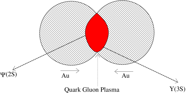
Figure 42: Au-Au collisions producing $\Psi(2S)$ and $\Upsilon(3S)$ from theQGP.

6.4 Conclusions for Heavy-quark state production in A-A collisions at $\sqrt{s_{pp}}$=200 GeV

The differential rapidity cross sections for $J/\Psi,\Psi(2S)$ and $\Upsilon(nS)(n=1,2,3)$ production via Cu-Cu and Au-Au collisions at RHIC (E=200 GeV) were calculated using $R_{AA}$, the nuclear modification factor, $N^{AA}_{bin}$ the binary collision number, and the gluon distribution functions. This should give some guidance for future RHIC experiments, although at the present time the $\Upsilon(nS)$ states cannot be resolved.

The ratio of the production of $\sigma(\Psi^{\prime}(2S))$, which in the mixed hybrid theory is 50% $c\bar{c}(2S)$ and 50% $c\bar{c}g(2S)$ with a $10\%$ uncertainty, to $J/\Psi(1S)$, which is the standard $c\bar{c}(1S)$, could be an important test of the production of the Quark-Gluon Plasma. Using the hybrid model and suppression factors from previous theoretical estimates and experiments on $\Upsilon(mS)$ state production at the LHC, the ratio of $\Psi^{\prime}(2S)$ to $J/\Psi(1S)$ production at RHIC via A-A collisions is estimated to be about $0.52\pm 0.05$. In future studies at BNL and the LHC-CERN the study of RHIC producing $\Psi^{\prime}(2S)$ and $\Upsilon(3S)$ mixed hybrid meson could be a method for determining the creation of the QGP.

6.5 $J/\Psi$ state production in Pb-Pb collisions at $\sqrt{s_{NN}}$=2.76 TeV

There have also been a number of experiments by the ALICE Collaboration on the production of $J/\Psi$ via Pb-Pb collisions at 2.76 TeV[60, 61, 62] which has measured $R_{AA}$ and other aspects of A-A collisions needed to establish the detection of the QGP. Since the present review is mainly focused on experimental tests of the mixed hybrid theory, with present detectors and also future LHC upgrades, we do not discuss these experimental publications in further detail.

7 Production of Charmonium and Upsilon States via Fragmentation

In the previous sections we reviewed the production of $c\bar{c}$ and $b\bar{b}$ states via p-p and A-A collisions. In this section we review the production of $|c\bar{q}>$ and $|b\bar{q}>$, with $q$ a light quark. Therefore the dominant octet processes illustrated in Figure 12, which produce $Q\bar{Q}$ states are not sufficient. To produce a $Q\bar{q}$ state, with $Q=c{\rm\;or\;}b$ and $q$ a light quark, one needs the quark fragmentation processes, which was introduced for the study of $Z^{0}$ (a weak gauge boson) decay[53]. This is illustrated in Figure 43.

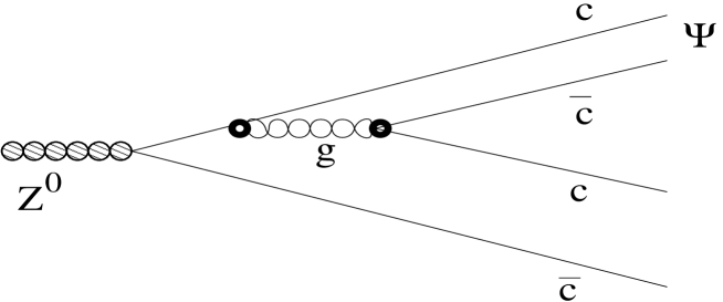
Figure 43: Quark fragmentation for $Z^{0}\rightarrow\Psi+c\bar{c}$

The fragmentation probability which is used in the production of D-mesons via p-p collisions discussed in the following subsection was calculated by Bratten $et.al.$[54]

Gluon fragmentation into heavy quarkonium calculated in Ref[55] is illustrated in Figure 44. Although it is important for some charmonium or bottonium state production, we do not use it in the present review.

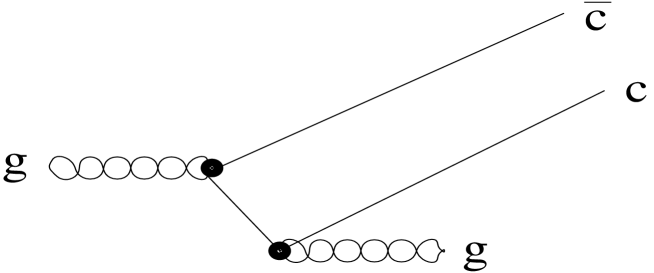
Figure 44: Gluon fragmentation into $c\bar{c}g$

7.1 D Production In p-p and d-Au Collisions

In this subsection the production of $D^{+}(c\bar{d}),D^{o}(c\bar{u})$ Charm mesons via unpolarized p-p and d-Au collisions at 200 GeV, based on recent research that has not yet been published[63], is discussed. The main new aspect of the present work is that while a gluon can produce a $c\bar{c}$ or $b\bar{b}$ state, it cannot directly produce a $c\bar{d}$. A fragmentation process converts a $c\bar{c}$ into a $c\bar{d}-d\bar{c}$, for example. We use the fragmentation probability, $D_{c\rightarrow c\bar{q}}$ of Bratten et. al.[54], illustrated in Figure 45.

Figure 45: Quark fragmentation for $Q^{*}\rightarrow(Q\bar{q})+q)$

7.1.1 Differential $pp\rightarrow DX$ cross section

Using what in Ref[20] is called scenerio 2, the production cross section with gluon dominance for DX is

$$\sigma_{pp\rightarrow Dx} = \int_{a}^{1}\frac{dx}{x}f_{g}(x,2m)f_{g}(a/x,2m)\sigma_{gg\rightarrow DX}\;,$$ (53)

with[54]

$$\sigma_{gg\rightarrow DX} = 2\sigma_{gg\rightarrow c\bar{c}}D_{c\rightarrow c\bar{q}}\;,$$ (54)

where $\sigma_{gg\rightarrow c\bar{c}}$ is similar to the charmonium production cross section in Ref[19] and $D_{c\rightarrow c\bar{q}}$ is the total fragmentation probability.

For $E=\sqrt{s}$=200 GeV the gluon distribution funtion is

$$f_{g}(y) = 1334.21-67056.5x(y)+887962.0x(y)^{2}$$ (55)

From Ref[54], using the light quark mass=(up quark mass+down quark mass)/2=3.5 Mev.

$$D_{c\rightarrow c\bar{q}} = 9.21\times 10^{5}\alpha_{s}^{2}|R(0)|^{2}/\pi\;,$$ (56)

in units of $(1/GeV^{3})$, with $\alpha_{s}=.26$. For a 1S state $|R(0)|^{2}=4/(a_{o})^{3}$. For a $c\bar{q}$ state, $(1/a_{o})=m_{q}\simeq 3.5$ MeV. Therefore,

$$|R(0)|^{2} \simeq 1.71\times 10^{-7}{\rm\;\;(GeV)^{3}}$$

$$D_{c\rightarrow c\bar{q}} \simeq 3.39\times 10^{-3}\;.$$ (57)

The calculation is similar to that in Ref[19].

$$\frac{d\sigma_{pp\rightarrow DX}}{dy} = Acc*f_{g}(x(y),2m)f_{g}(a/x(y),2m)\frac{dx(y)}{dy}\frac{1}{x(y)}D_{c\rightarrow c\bar{q}}\;,$$ (58)

with $y$ and $x(y)$ defined above and $Acc$ is the matrix element for charmonium production[19] with an effective mass $ms$=1.5 GeV

$$Acc = 7.9*10^{-4}nb\;.$$ (59)

From Eqs(58,59) one finds $\frac{d\sigma_{pp\rightarrow DX}}{dy}$ shown in Figure 44 after the next subsubsection.

7.1.2 Differential $dAu\rightarrow DX$ cross section

In this subsubsection we estimate the production of $D^{+},D^{0}$ from d-Au collisions, using the methods given in Ref.[33] for the estimate of production of $\Psi$ and $\Upsilon$ states via Cu-Cu and Au-Au collisions based on p-p collisions.

The differential rapidity cross section for D+X production via d-Au collisions is given by $\frac{d\sigma_{pp\rightarrow DX}}{dy}$ with modification described in Ref.[33] for Cu-Cu and Au-Au collisions:

$$\frac{d\sigma_{dAu\rightarrow DX}}{dy} = R_{dAu}N^{dAu}_{coll}\left(\frac{d\sigma_{pp\rightarrow DX}}{dy}\right)\;,$$ (60)

where $R_{dAu}$ is the nuclear-modification factor, $N^{dAu}_{coll}$ is the number of binary collisions, and $\left(\frac{d\sigma_{pp\rightarrow DX}}{dy}\right)$ is the differential rapidity cross section for $DX$ production via nucleon-nucleon collisions in the nuclear medium.

$\left(\frac{d\sigma_{pp\rightarrow DX}}{dy}\right)$ is given by Eq(58) with $x(y)$ replaced by the function $\bar{x}$ (see (Eq(6)), the effective parton x in the nucleus Au.

In Ref.[37] the quantities $R_{dAu}$ and $N^{dAu}_{coll}$ (called $R_{dA}$ and $<N_{coll}>$ in that article) were estimated from experiments on p+p and d+Au collisions. From that reference $R_{dAu}\simeq 1.0$ and $N^{dAu}_{coll}\simeq 10.0$.

From Eqs(58,60), one obtains the differential rapidity cross section for D+X production via dAu collisions. In Figure 46 $\frac{d\sigma_{pp\rightarrow DX}}{dy}$ and $\frac{d\sigma_{dAu\rightarrow DX}}{dy}$ are shown

Figure 46: $d\sigma/dy$ with E=200 GeV for (A) unpolarized p-p collisions and (B) d-Au collisions producing D+X

A number of experiments have measured $\sigma_{c\bar{c}}$ cross sections at $\sqrt{s_{pp}}$=200 GeV[56, 57, 46, 64]. Theoretical estimates of heavy quark state production via p-p collisions at RHIC and LHC energies were made almost two decades ago[65]. More recently estimates of $D$ production were made from data on d-Au collisions at $\sqrt{s_{NN}}$= 200 GeV[66]. Experimental measurements of $D^{+},D^{-},D^{0}$ production via p-p and d-Au collisions are expected in the future.

8 Sivers and Collins Fragmentation Functions

The E1039 Collaboration, see Ref[67] for the Letter of Intent, plans to carry out a Drell-Yan experiment with a polarized Proton target, with the main objective to measure the Sivers function[68]. This Letter of Intent has motivated this brief review of Sivers and Collins symetries and fragmentation functions.

A number of Deep Inelastic Scattering experiments[69, 70, 71] have measured non-zero values for the Sivers Function. See these references for references to earlier experiments. Another important function is the Collins fragmentation function[72], which describes the fragmentation of a transversly polarized quark into an unpolarized hadron, such as a pion. The Sivers and Collins functions are defined by the target assymmetry, $A(\phi,\phi_{S}$), in the scattering of an unpolarized lepton beam by a transversely polarized target[71]:

$$A(\phi,\phi_{S}) \simeq A_{C}(\phi,\phi_{S})sin(\phi+\phi_{S})+A_{S}(\phi,\phi_{S})sin(\phi-\phi_{S})\;,$$ (61)

where $A_{C},A_{S}$ are the Collins,Sivers functions with $\phi$ the azimuthal angle and $\phi_{S}$ the aximuthal angle with respect to the lepton beam.

8.1 Sivers Function

The Sivers term of the cross section for the production of hadrons using an unpolarized lepton beam on a transversely polarized target is[69]

$$\sigma_{S}(\phi,\phi_{S}) = \sigma_{UU}S_{T}(x)[2n(<sin(\phi-\phi_{S})>_{UT}\times sin(\phi-\phi_{S})+...]\;,$$ (62)

where $\phi$ and $\phi_{S}$ were defined above. $\sigma_{UU}$ is the $\phi$- independent part of the polarization-independent cross section; and $UT$ denotes the unpolarized beam with transverse target polarization w.r.t. the virtual photon direction. $S_{T}(x)$ is the Sivers Function with $x=-q^{2}/(2P\cdot q)$ and $P$ is the four-momentum of the target proton. As mentioned above, a number of Deep Inelastic Scattering experiments have measured $S_{T}(x)$ and obtained non-zero values. See, e.g., Ref[69] for a discussion of the Sivers Function in terms of experimental cross sections.

8.2 Collins Fragmentation Function

The definition of the Collins Function is similar to that of the Sivers Function in Eq(62[73]:

$$\sigma_{C}(\phi,\phi_{S}) \propto F_{UU}(1+A_{UT}\times sin(\phi+\phi_{S}))\;,$$ (63)

with $\phi$ and $\phi_{S}$ defined above, $F_{UU}$ the spin-averaged structure function, and $A_{UT}$ the asymmetry that can be calculated from quark distribution and fragmentation, which is now discussed briefly .

From Ref[74] the fragmentation function to produce a hadron, $h$ from a transversely polaried quarek in $e^{+}e^{-}$ annihilation is

$$D_{hq^{\uparrow}}(z,k_{T}^{2}) = D^{q}(z,k_{T}^{2})+H^{q}(z,k_{T}^{2})\frac{k\times k_{T}/k)\cdot s_{q}}{zM_{h}}\;,$$ (64)

where $M_{h}$ is the hadron mass, k is the quark momentum, $s_{q}$ is the quark spin vector, $k_{T}$ the hadron momentum transverse to k, and z the light-cone momentum fraction of h wrt the fragmenting quark. The Collins fragmentation function is $H^{q}$.

The calcultion of $D_{hq^{\uparrow}}$ is similar to the fragmentation function for D production in p-p collisions[63] discussed above. An estimate of the Collins Fragmentation Function is being carried out[75].

9 Brief Overview

The theoretical basis for production of heavy quark states via p-p collisions, using the standard model for $J/\Psi,\Upsilon(1S),\Upsilon(2S)$ states and a mixed hybrid theory for $\Psi(2S),\Upsilon(3S)$ using QCD and QCD Sum Rules has been established by comparison with many experiments. For detection of the Quark-Gluon plasma, a main objective of RHIC and an important objective for the LHC, production of heavy quark states via A-A collisions is required. This is much more complicated, but there has been a great deal of progress in both experiment and theory. The detection of the Quark-Gluon Plasma via A-A collisions is closer to realization with this improved theory.

Also, the theory of production of open charm and bottom meson via p-p and A-A collisions is now greatly improved using the theory of Fragmentation. Deep inelastic experiments for measuring the Sivers and Collins Fragmentation functionns are being carried out and are planned for the future.

Acknowledgements

Author D.D. acknowledges the facilities of Saha Institute of Nuclear Physics, Kolkata, India. Author L.S.K. acknowledges support from the P25 group at Los Alamos National laboratory.

References

- [1] D. Gross and F. Wilczek, Phys. Rev. Lett. 30, 1343 (1973)
- [2] S. Weinberg, Phys. Rev. Lett. 31, 494 (1973)
- [3] H. Fritzsch, M. Gell-Mann, and H. Leutwyler, Phys. Lett. bf 47B,365 (1973)
- [4] Ta-Pei Cheng and Ling-Fong Li, “Gauge theory of elementary particle physics”, Oxford Universityese Press (1984)
- [5] Edward V. Shuryak, Phys. Reports, 61, 71 (1980)
- [6] Leonard S Kisslinger, “Astrophysics and the Evolution of the universe”, World Scientific Publishing Co. (2014)
- [7] S. Chatrchyan (CMS Collaboration), Phys. Rev. D 78, 092007 (2014)
- [8] G. Add (ATLAS Collaboration) Phys. Rev. D 90, 052004 (2014)
- [9] Zhou Li-juan, Ma Wei-xing, Leonard S. Kisslinger, J. Mod. Phys. 3, 1172 (2012)
- [10] H. Vogel, Proceedings of 4th Flavor Physics and CP Violation Conference (FPCP’06) (2006)
- [11] M.A. Shifman, A.I. Vainstein and V.I. Zakharov, Nucl. Phys. B147, 385; Nucl. Phys. B147 448 (1979)
- [12] L.S. Kisslinger, Phys. Rev. D 79, 114026 (2009)
- [13] CDF Collaboration,arXiv:hep-ex/9412013; Phys. Rev. Lett. 79, 578 (1997)
- [14] P.L Cho and A.K. Leibovich, Phys. Rev. D 53, 150 (1996)
- [15] E. Braaten and Y-Q Chen, Phys. Rev. D 54, 3216 (1996)
- [16] E. Braaten and S. Fleming, Phys. Rev. Lett. 74, 3327 (1995)
- [17] P.L Cho and A.K. Leibovich, Phys. Rev. D 53, 6203 (1996)
- [18] R. Baier and R. Ruckl, Z. Phys. C 19, 251 (1983)
- [19] L.S. Kisslinger, M.X. Liu, and P. McGaughey, Phys. Rev. D 84, 114020 (2011).
- [20] G.C. Nayak and J. Smith, Phys. Rev. D 73, 014007 (2006)
- [21] E. Merzbacher, “Quantum Mechanics”, John Wiley and Sons (1970)
- [22] CTEQ6: hep.pa.msu.edu/cteq/public/cteq6.html
- [23] F. Cooper, M.X. Liu, and G.C. Nayak, Phys. Rev. Lett.93, 171801 (2004)
- [24] G. Moreno , Phys. Rev. D 43, 2815 (1991)
- [25] P. L. McGaughey , Phys. Rev. D 50, 3038 (1994)
- [26] Leonard S. Kisslinger and Debasish Das, Mod. Phys. Lett A 28, 1350067 (2013)
- [27] Leonard S. Kisslinger,MPLA-D-12-00057(2012)
- [28] R. Aaij et al. [LHCb Collaboration], Eur. Phys. J. C 72, 2025 (2012).
- [29] Leonard S. Kisslinger and Debasish Das, Mod. Phys. Lett A 28, 1350120 (2013)
- [30] Leonard S. Kisslinger and Debasish Das, Mod. Phys. Lett A 29, 1450082 (2014)
- [31] Leonard S. Kisslinger and Debasish Das, arXix:1501.03128; Int.J.Mod. Phys.E 24, 1550038 (2015)
- [32] Leonard S. Kisslinger and Debasish Das, in preperation (2015).
- [33] L.S. Kisslinger, M.X. Liu, and P. McGaughey, Phys. Rev. C 89,024914 (2014)
- [34] The ALICE Collaboration, Eur. Phys. J. C 74, 2974 (2014)
- [35] The ATLAS Collaboration, Phys. Rev. D 87, 052004 (2013)
- [36] The LHCb Collaboration, JHEP 1511, 103 (2015)
- [37] A. Adare , et. al., Phys. Rev. Lett. 112, 252301 (2014)
- [38] K. Adcox (PHENIX Collaboration) Phys. Rev. Lett. 88, 022301 (2002)
- [39] C. Adler (STAR Collaboration), Phys. Rev. Lett. 89, 202301 (2002)
- [40] R. Vogt, Phys. Rev. C 81, 044903 (2010)
- [41] Risha Sharma and Ivan Vitev, Phys. Rev. C 87, 044905 (2013)
- [42] A.D. Frawley, T. Ullrich, and R. Vogt, Phys Rep. 462, 125 (2008)
- [43] B.I. Abelev (STAR Collaboration), Phys. Rev. C 80, 041902 (2009)
- [44] A. Adare (PHENIX Collaboration) Phys. Rev. Lett. 101, 122301 (2008)
- [45] A. Adare (PHENIX Collaboration) Phys. Rev. Lett 98, 172301 (2007)
- [46] B.I. Abelev (STAR Collaboration) Phys. Rev. Lett. 98, 192301 (2007)
- [47] I. Vitev, T. Goldman, M.B. Johnson, and J.W. Qiu, Phys. Rev. D 74, 054010 (2006)
- [48] R. Sharma, I. Vitev, and B-W. Zhang, Phys. Rev. D 80, 054902 (2009)
- [49] J.W. Qiu and I. Vitev, Phys. Rev. Lett. 93, 262301 (2004)
- [50] The CMS Collaboration, Phys.Rev.Lett.107, 052302 (2011)
- [51] A. Adare et al (PHOENIX Collaboration), Phys. Rev. D 85, 092004 (2012)
- [52] S. Chatrchyan (CMS Collaboration) Phys. Rev. Lett. 109, 222301 (2012)
- [53] Eric Braaten, Kingman Cheung, and Tzu Chiang Yuan, Phys. Rev D 48, 4230 (1993)
- [54] Eric Bratten, Kingman Cheng, Sean Fleming, Tzu Yuan, Phys. Rev. D 51, 4819 (1995)
- [55] Eric Braaten and Tzu Chiang Yuan, Phys. Rev. Lett. 71, 1673 (1993)
- [56] A. Adare, et. al., PHENIX Collaboration, Phys. Rev. Lett. 97,252002 (2006)
- [57] S.S. Adler, , PHENIX Collaboration, Phys. Rev. D 76, 092002 (2007)
- [58] F. Karsch, D. Kharzeev and H. Satz, Phys. Lett. B 637, 75 (2006)
- [59] S. Baumgart (STAR), arXiv:0709.4223/nucl-ex
- [60] B. Abelev (ALICE Collaboration), Phys. Rev. Lett. 109, 072301 (2012)
- [61] Debasish Das (ALICE Collaboration), arXiv:1212.2704/nucl-ex (2012)
- [62] ALICE Collaboration, Phys. Lett. 743, 314 (2014)
- [63] Leonard S. Kisslinger, Miong X. Liu and Patrick McGaughey, arXiv:1507.07252 [hep-ph] (2015)
- [64] A. Adare , PHENIX Collaboration, Phy. Lett. B 670, 313 (2009)
- [65] R.V. Gavai, S. Gupta, P.L. McGaughey, E. Quack, P.V. Ruuskanen, R. Vogt and Xin-Nian Wang, Int. J. Mod. Phys. A 10, 2999 (1995)
- [66] J. Adams, , STAR Collaboration, Phys. Rev. Lett. 94, 062301 (2005)
- [67] https://www.fnal.gov/directorate/program_planning/ June2013PACPublic/P-1039_LOI_polarized_DY.pdf
- [68] Dennis Sivers, Phys. Rev. D 41, 83 (1990)
- [69] A. Airapetian et. al. (HERMES Collaboration), Phys. Rev. Lett. 103, 152002 (2009)
- [70] M. Alekseev et. al. (COMPASS Collaboration), Phys. Lett. B 673, 127 (2009)
- [71] X. Qian et. al. (JLAB Hall A Collaboration), Phys. Rev. Lett. 107, 072003 (2001)
- [72] J.C. Collins, Nucl. Phys. B 396, 161 (1993)
- [73] Zhong-Bo Kang, Alexi Prokudin, Peng Sun, and Feng Yuan, Phys. Rev. D 91, 071501 (2015)
- [74] Alessandro Bacchetta, Leonard P. Gamberg, Gary R. Goldstein, Asmita Mukherjee, Phys. Lett B 659, 234 (2008)
- [75] L.S. Kisslinger, in progress (2016)