The Far-Infrared-Radio Correlation in MS0451-03

Abstract

We present a multi-wavelength analysis of star-forming galaxies in the massive cluster MS0451.6-0305 at z $\sim$ 0.54 to shed new light on the evolution of the far-infrared-radio relationship in distant rich clusters. We have derived total infrared luminosities for a spectroscopically confirmed sample of cluster and field galaxies through an empirical relation based on $Spitzer$ MIPS 24 $\upmu$m photometry. The radio flux densities were measured from deep Very Large Array 1.4 GHz radio continuum observations. We find the ratio of far-infrared to radio luminosity for galaxies in an intermediate redshift cluster to be $q_{\rm FIR}$ = 1.80$\pm$0.15 with a dispersion of 0.53. Due to the large intrinsic dispersion, we do not find any observable change in this value with either redshift or environment. However, a higher percentage of galaxies in this cluster show an excess in their radio fluxes when compared to low redshift clusters ($27^{+23}_{-13}\%$ to $11\%$), suggestive of a cluster enhancement of radio-excess sources at this earlier epoch. In addition, the far-infrared-radio relationship for blue galaxies, where $q_{\rm FIR}$ = 2.01$\pm$0.14 with a dispersion of 0.35, is consistent with the predicted value from the field relationship, although these results are based on a sample from a single cluster.

1 Introduction

Radio continuum emission from normal star-forming galaxies can be a powerful tracer of recent star formation activity (Condon, 1992). The radio luminosities at 1.4 GHz are tightly correlated with the far-infrared luminosities for various galaxy types (e.g. van der Kruit, 1971; Helou et al., 1985; Condon et al., 1991) over a wide range of redshift (e.g. Garrett, 2002; Appleton et al., 2004; Sargent et al., 2010a; Jarvis et al., 2010; Ivison et al., 2010a).

The correlation is believed to be driven by the internal star formation rate. Radio emission from these galaxies are predominantly produced from the synchrotron emission of cosmic-ray electrons accelerated in supernova shocks. The infrared emission is due to ultraviolet light from young massive stars that is absorbed and re-radiated by dust (Condon, 1992). However, it is still unclear what maintains this strong correlation seen over such a wide range of galaxies (Murphy, 2009).

The relationship shows lower far-infrared to radio luminosity ratios in galaxy clusters than that found in the field (Andersen & Owen, 1995; Reddy & Yun, 2004) with much of the variation coming from a subset of objects with large deviations from the relationship (Miller & Owen, 2001). A number of different processes drive the evolution of galaxies in clusters such as gravitational interactions and ram pressure (see e.g., Boselli & Gavazzi, 2006, for a review), and result in transforming blue, star-forming galaxies into the ubiquitous red, quiescent galaxies that dominate cluster populations today. These physical processes have been invoked to explain the differences seen in the far-infrared-radio relationship as measured between the cluster and field (Murphy et al., 2009).

However, little work has been done at higher redshifts where we see an increase of star-forming galaxies (Butcher & Oemler, 1984), transitional galaxies like E+A (Barger et al., 1996), and AGN (Martini et al., 2009) in galaxy clusters. Despite studies looking at the multi-wavelength properties of galaxies in distant clusters (e.g. Best et al., 2002; Saintonge et al., 2008), no systematic study has been made of the far-infrared-radio relationship in these clusters, and so, the present work is an unique opportunity to explore part of parameter space in redshift and environment that has not previously been probed.

This work aims to measure the far-infrared-radio relation in the massive galaxy cluster MS0451.6-0305 (hereafter, MS0451-03) to test how this relationship changes at intermediate redshift between the field and a high-density cluster environment. The properties of the cluster are summarised as follows: MS0451-03 is a massive (M₂₀₀ $\sim$ 3$\times$10¹⁵ M_⊙), X-ray luminous (L${}_{\rm x}^{\rm bol}$=4$\times$10⁴⁵ erg s^-1), and large (R₂₀₀ $\sim$ 2.5 Mpc) cluster at $z$=0.538 (see Crawford et al., 2009, Table 1).

The paper is organised as follows. Section 2 presents the VLA 1.4 GHz radio continuum observations and provides our radio data reduction and analysis. Section 3 presents the $Spitzer$ MIPS observations along with the infrared (IR) photometry. Section 4 and Section 5 describe our sample selection procedure and methodology. Section 6 presents our results. Finally, Section 7 and Section 8 discuss and summarise our findings and then suggest some future work. Throughout this paper, we adopt $\rm H_{0}$ = 71 km s^-1 Mpc^-1, $\Omega_{\rm m}$ = 0.27 and $\Omega_{\rm DE}$ = 0.73.

2 VLA Observation & Data Reduction

2.1 VLA Observations

Very Large Array (VLA) observations at 1.4 GHz were retrieved from the National Radio Astronomy Observatory (NRAO) data archive. The data were all taken in wide field ”pseudo-continuum mode” which consists of 25 MHz bandwidth observations acquired at two intermediate frequencies (IFs) centred at 1364.9 MHz and 1435.1 MHz. Each IF consists of seven 3.125 MHz channels and provides both left and right circular polarisation. Flux and phase calibration were tracked using flux calibrators (0137+331 or 3C 48) and a phase calibrator (0503+020), respectively. The summary of each archival VLA 1.4 GHz radio continuum observation is provided as follows:

1. BnA-array data (hereafter, B-array) were obtained in June 9^th-10^th 2002, that have a sensitivity as reported in the observing log of $\sim$ 0.052 mJy beam^-1 with on source target durations worth a total observing time of 7.8 hours, where data were recorded every 10 s.

2. A-array data were obtained on February 5^th-6^th and 10^th-11^th 2006, that have a sensitivity as reported in the observing log of $\sim$ 0.04 mJy beam^-1 with on source target durations worth a total observing time of 12.8 hours, where data were recorded every 3.3 s.

2.2 VLA Data Reduction

The radio continuum data reduction and analysis were entirely carried out using the NRAO Astronomical Image Processing System ($\cal AIPS\/$) package (Greisen, 2003). Our data reduction followed the standard calibration procedures that include data inspection, exploring visibilities, flagging, phase and flux calibrations. For both B-array and A-array, removal of corrupted data and calibration were performed in a similar manner. The final calibration solutions were applied individually to the different epochs. We combined the two fully calibrated UV data sets and used wide field imaging techniques to image a large field of view beyond the primary beam. We put facets on all bright sources within one square degrees of the pointing centre to properly account for flux and diminish sidelobe contamination.

Unlike the reduction procedures of Berciano Alba et al. (2010) of this cluster for their studies of sub-mm emissions from galaxies, we treated the B-array observations as single epoch. No self-calibration was applied. The noise in our combined image was found to be comparable to previously reduced data in the literature. Furthermore, no convolutional artifacts were found around the point sources. The A-array observations were run during the upgrade of the VLA with a mix of EVLA with VLA antennas used during the observing period. As a result, we discarded data from all three EVLA antennas because they could not be calibrated with the VLA antennas.

The A-array data set has higher resolution and is thus quite sensitive to point sources and small structures. Additionally, it dominates the total integrated time on source. As a result, any mapping parameters for the final radio map are dictated by the A-array. Facets for wide field imaging were based on bright sources found by $\cal AIPS\/$ SETFC routine, resulting in 61 facets that were auto-generated for the targeted field coverage. Each facet was set to the same pixel scaling of 0.3” and 4096$\times$4096 pixels in size. For all fields, during the cleaning process, cleaned regions were limited to each bright source by putting a clean box around it. The final clean maps have a convolved beam size (HPBW) of 1.99”$\times$1.63” at a position angle of 0.56. The final flattened radio map was imaged within a field of view coverage of 0.75^∘$\times$0.75^∘ with a pixel scaling of 0.3” and has an RMS noise level of 11.98 $\upmu$Jy beam^-1 as measured using $\cal AIPS\/$ TVSTAT. We define our detection limit for this image as being 36 $\upmu$Jy, which is 3 times the RMS found in a single beam.

2.3 Radio Sources Extraction and Cataloguing

Our radio source catalogue was generated using the $\cal AIPS\/$ task SAD by running this routine in the signal-to-noise mode (S/N$\geq$3). The $\cal AIPS\/$ task RMSD was used to create an RMS noise map where calculation of the noise map was performed within a 30” diameter circular aperture corresponding to 100 neighbour pixels (see e.g., Morrison et al., 2010; Wold et al., 2012). Source classification and flux were assigned based on the method adopted by Owen & Morrison (2008) using the best-fit major axis value. For the resolved sources (i.e., sources that have lower-limit best-fit major axis greater than zero), the total flux densities are directly assigned to the sources while peak flux densities are equal to the total flux densities for the unresolved sources.

We re-measured the 1.4 GHz flux density of fifteen sources published in Wardlow et al. (2010) to verify the quality of our measurements. Within the estimated uncertainty range, we have found a very good consistency between the two measurements with a mean offset of 1.6 $\upmu$Jy and a dispersion of 5.5 $\upmu$Jy (i.e., within the RMS noise of our map).

3 Spitzer Observation & Photometry

3.1 Observations

A Multiband Imaging Photometer for $Spitzer$ (MIPS; Rieke et al., 2004) 24 $\upmu$m imaging mosaic for this field was retrieved from the $Spitzer$ Enhanced Imaging Products (SEIP) data archive. This high level product consists of a combination of multiple programs and has a field of view of $\sim$ 0.3^∘$\times$0.3^∘. The mean integration time of the MIPS 24 $\upmu$m super mosaic imaging is 1637 seconds per pixel. The MIPS 24 $\upmu$m data has a median pixel scaling of 2.45” and a mean FWHM of 5.9”. The RMS noise of the image was $\sim$ 26 $\upmu$Jy.

Additionally, $Spitzer$ super mosaics of the Infrared Array Camera (IRAC; Fazio et al., 2004) at 3.6 $\upmu$m, 4.5 $\upmu$m, 5.8 $\upmu$m, 8.0 $\upmu$m were also retrieved. IRAC observations were used for sample selection and matching. The IRAC images have a median pixel scaling of $\sim$ 1.2” and the image mean FWHM is 1.66”, 1.72”, 1.88”, and 1.98”, respectively. The RMS noise of the images were $\sim$ 10 $\upmu$Jy.

3.2 Far-Infrared Data at Longer Wavelength

No $Spitzer$ MIPS super mosaics imaging at 70, 160 $\upmu$m are available in the SEIP data archive for the cluster. However, $Spitzer$ MIPS imaging at 24, 70 and 160 $\upmu$m for the cluster are available in the Spitzer Heritage Archive (SHA) but they have shallower depth and smaller field than the 24 $\upmu$m images. Due to these limitations, none of the confirmed cluster sources were matched with our 24 $\upmu$m catalogue. We have examined data from the recently available Herschel observations in the field for this cluster which consists of both PACS/PACS Evolutionary Probe (PEP) (Lutz et al., 2011; Magnelli et al., 2013) and the SPIRE/Herschel Multi-tiered Extragalactic Survey (HerMES) (Oliver et al., 2012; Smith et al., 2012). The PACS data do not fully cover our field of view and we were only able to detect two sources in the SPIRE observations. As the Herschel data are not expected to significantly modify our results and due to the small number of sources with data, we did not attempt any further analysis using this data. The implications for only including 24 $\upmu$m observations are further discussed in §6.2.

3.3 Photometry

Optical coordinates (see §4) were used to perform aperture photometry on the $Spitzer$ observations. Aperture photometry was done using APEX (Makovoz & Marleau, 2005, $Spitzer$ MOPEX). The aperture size was set to a radius of 5.31” in the MIPS 24 $\upmu$m imaging, which is the optimal aperture size suggested for point sources based on the pixel sampling of the MIPS 24 $\upmu$m PSF. Clusters sources are expected to be essentially unresolved at this redshift in the MIPS 24 $\upmu$m data. We re-measured the MIPS 24 $\upmu$m flux density of the sources published in Wardlow et al. (2010) to verify the quality of our measurements. For 15 sources published in Wardlow et al. (2010), we have found a very good consistency between the two measurements with a mean offset of 16.8 $\upmu$Jy and a dispersion of 46 $\upmu$Jy.

4 Sample Selection

Our galaxy sample was drawn based on spectroscopic data of the cluster MS0451-03 (Moran et al., 2007; Crawford et al., 2011) and includes 350 cluster sources. Cluster membership was determined through a “shifting-gapper” analysis (see, Crawford et al., 2014) similar to Fadda et al. (1996) which determined membership through analysis of the radius-velocity diagram. Apart from the confirmed cluster galaxies, our sample also contains 1107 field galaxies that have secure spectroscopic redshift.

Photometry was performed on the MIPS 24 $\upmu$m image for all spectroscopic sources in our sample appearing in those images. Sources outside of the MIPS 24 $\upmu$m image were removed from our sample along with sources with flux densities detected at $<$ 3$\upsigma$ level. The final catalogue of sources with secure spectroscopic redshifts and IR photometry comprises 155 cluster galaxies and 479 field galaxies.

We matched the radio sources to this catalogue. A matching radius of 2” was used. Any unambiguous identifications were discarded from the final catalogue. We were able to securely match 12 out of 155 cluster member galaxies and 27 out of 479 field galaxies.

Our full sample of matched sources is presented in Table 1 for cluster galaxies and Table 2 for the field galaxies. The tables include ID, RA, DEC, redshift, radius, 1.4 GHz flux density and its uncertainty, radio luminosity, MIPS 24 $\upmu$m flux density and its uncertainty, and IR luminosities. As in Yun et al. (2001) and Reddy & Yun (2004), we have not a priori excluded AGN sources so our selection is a heterogeneous sample of star forming galaxies and AGN. The derivation of the intrinsic properties is presented in § 5.

5 Methods

5.1 The Radio Luminosity

We converted the integrated radio flux densities ($\rm S_{1.4\rm GHz}$) into rest frame radio luminosities ($\rm L_{1.4\rm GHz}$) using:

$$\rm L_{1.4GHz}(W\ Hz^{-1})=\left(\frac{4\pi[D_{L}(z)]^{2}}{(1+z)^{1-\alpha}}\right)\times S_{1.4\rm GHz}$$ (1)

where S_1.4GHz is the flux density at 1.4 GHz in Jy, and D${}_{L}(z)$ is the luminosity distance at the redshift of the sources. The $K$-correction 1/(1+z)^(1-α) consists of 1/(1 + z)^-α and 1/(1 + z) terms that are the “colour” and bandwidth correction, respectively (Morrison et al., 2003). The radio spectral index $\alpha$ is the power law slope of the synchrotron radiation, and is defined as S_ν$\sim$$\upnu^{-\alpha}$. We assumed $\alpha$ $\sim$ 0.8 for normal star-forming galaxies of Condon (1992).

5.2 The Infrared Luminosities

Since we do not have sufficient information to fit templates to individual galaxies, we used a simple recipe derived from Rieke et al. (2009) for converting between observed 24 $\upmu$m flux density and L_24μm based on the best-fit SFR calibration. This is based on Equation 10-14 and Table 1 from Rieke et al. (2009). The conversion is as follows:

$$L{(24\rm\upmu m,L_{\odot})}=\frac{\rm 10^{A(z)+B(z)\times(log(4\pi D_{L}^{2}\ f_{24,obs})-53)}}{7.8\times 10^{-10}};\\ {\rm for,}\ 6\times 10^{8}L_{\odot}\leq L_{24\rm\upmu m}\leq 1.3\times 10^{10}L_{\odot}$$ (2)

$$L{(24\rm\upmu m,L_{\odot})}=\left(\frac{\rm 10^{A(z)+B(z)\times(log(4\pi D_{L}^{2}\ f_{24,obs})-53)}}{7.8\times 10^{-10}\times(7.76\times 10^{-11})^{0.048}}\right)^{0.954};\\ {\rm if,}\ L_{24\rm\upmu m}>1.3\times 10^{10}L_{\odot}$$ (3)

where $D_{L}$ is the luminosity distance in cm and $f_{\rm 24,obs}$ is the flux density at 24 $\upmu$m in Jy. The coefficients A(z) and B(z) are redshift-dependent and can be obtained by interpolating the values in Table 1 of Rieke et al. (2009); or see values are provided in our Table A1 in the Appendix A.

In addition to L_24μm, we also calculate the IR luminosities L_TIR, L_60μm, and L_FIR to allow a comparison of our measurements to other works. We adopt the definition from Rieke et al. (2009) that L_TIR is the luminosity between L(TIR; 8–1000 $\upmu$m) and we adopt the definition of L_FIR from Helou et al. (1985) as L(FIR; 42–122 $\upmu$m). We provide the details of these transformations in Appendix A.

We also attempted to determine L_TIR based on fitting the spectral energy distribution (SED) using CIGALE (Noll et al., 2009). The photometric catalogues were fit to synthetic template spectra compiled from Maraston (2005) that incorporate the dust emission model of Dale & Helou (2002). The total infrared luminosities were then derived from the parameters of the best-fit model. Due to lacking suitable measurements in bandpasses that are redward of 24 $\upmu$m, the scarcity of data points, and the large parameter space of models, our measurements of the total IR luminosity L_TIR were poorly constrained. We thus limited any further analysis to the empirically determined L_TIR.

5.3 The IR to Radio Luminosity Ratio

We characterised the quantitative measure of the far-infrared-radio relation by calculating the median logarithmic ratio of IR and radio luminosity ($q$). The luminosity ratio was estimated using the commonly used equation of Helou et al. (1985) as follows:

$$q=\rm log\left(\frac{L}{3.75\times 10^{12}\ \rm W}\right)-log\left(\frac{L_{\rm 1.4GHz}}{\rm W\ Hz^{-1}}\right)$$ (4)

where L_1.4GHz is the rest frame radio luminosity calculated from Equation 1 in W Hz^-1. L is our infrared luminosity in W. The subscript of $q$ indicates which infrared luminosity is being used (i.e., q_TIR is for L_TIR). For calculating $q_{24}$, the constant used to normalise the infrared luminosity was $1.25\times 10^{13}$.

6 Results

Our primary aim is to compare the infrared-radio relationship in an intermediate redshift cluster to nearby clusters, and to do so, we will be comparing our results to the lower redshift measurements of Reddy & Yun (2004). As their results are reported in L_60μm and q_FIR within L(FIR; 42–122 $\upmu$m), we transform our L_24μm results into comparable bands. We report the luminosities for all the cluster sources in Table 1 and field sources in Table 2.

6.1 Far-Infrared-Radio Relation

The relationship between the rest frame radio luminosity at 1.4 GHz (L_1.4GHz) against the IR luminosity (L_60μm) is shown in Figure 1. The solid line indicates the formal linear least-square fit of the cluster galaxies of Reddy & Yun (2004) while the field relation from Yun et al. (2001) is drawn using the dashed line. Most of our cluster sources are consistent with these relationships. As indicated in the dash-dotted lines in Figure 1, our cluster galaxies IR luminosity and radio luminosity lower limits are log L_60μm = 10.21 and log L_1.4GHz = 22.6, respectively. For comparison, our lower limits are higher than the low redshift cluster galaxies (log L_60μm = 8.92, log L_1.4GHz = 20.47) of Reddy & Yun (2004).

We split our sample into blue cloud (BC) and red sequence (RS) galaxies following the definition in Crawford et al. (2011) for both cluster and field samples. In all Figures, red and blue colours indicate sources that have secure photometric measurements from our imaging data, while grey colour represents sources with unknown photometric classification. The number of sources that have secure photometric classification is 11 of 12 cluster sources and 13 of 27 field sources. For any values given for these populations, we only use sources with secure photometric measurements. For all other values reported in this paper, we calculate them based on the full cluster or field sample.

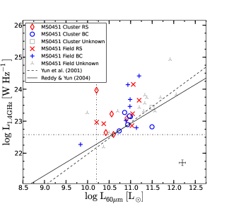
Figure 1: The 20 cm radio continuum luminosity (L_1.4GHz) against the IR luminosity (L_60μm). Red colour indicates red sequence (RS) galaxies while blue colour represents blue cloud (BC) galaxies. RS field galaxies are plotted in cross symbols, while BC field galaxies are drawn in plus symbols. Grey colour represents sources with unknown photometric classification. The solid and dashed lines indicate the formal linear least-square fit (log L_60μm = 8.92 luminosity cutoff) of the low redshift cluster galaxies from Reddy & Yun (2004) and field galaxies relation in Equation 4 of Yun et al. (2001). The error bars correspond to average 1$\upsigma$ errors.

In Figure 2, we present the far-IR luminosity (L_FIR) to radio luminosity ($\rm L_{1.4\rm GHz}$) ratio ($q_{\rm FIR}$) versus L_60μm. The solid gray line delineates our sample limiting magnitude. The mean $q_{\rm FIR}$ for the cluster population is $q_{\rm FIR}$ = 1.80$\pm$0.15 with a dispersion of 0.53, while field galaxies have $q_{\rm FIR}$ = 1.62$\pm$0.09 with a dispersion of 0.45. Our cluster value is consistent with Reddy & Yun (2004) value of $q_{\rm FIR}$ = 2.07$\pm$0.07 with a dispersion of 0.74. Our field value is lower, but due to the large intrinsic dispersion, we cannot firmly comment on its inconsistency with values found in similar works such as Yun et al. (2001) of $q_{\rm FIR}$ = 2.34$\pm$0.01 with a dispersion of 0.26. In addition to Reddy & Yun (2004) and Yun et al. (2001), our mean $q_{\rm FIR}$ values are comparable with other works (Andersen & Owen, 1995; Miller & Owen, 2001; Murphy et al., 2009; Garrett, 2002; Kovács et al., 2006; Sajina et al., 2008); see Table 4 for values from each of the surveys.

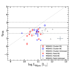
Figure 2: The logarithm of the far-IR luminosity to 1.4 GHz radio continuum luminosity ratio ($q_{\rm FIR}$) versus the IR luminosity (L_60μm). The nominal value of $q_{\rm FIR}$ for field galaxies ($q_{\rm FIR}$=2.34) is plotted in the solid black horizontal line. The criteria for both delineating the radio-excess ($q_{\rm FIR}$$\leq$1.64) and IR-excess ($q_{\rm FIR}$$\geq$3.04) are shown in the dashed lines. The error bars correspond to average 1$\upsigma$ errors. The solid gray line represents our sample limiting flux.

We also compare our other measurements to other works as well. For comparison, we found mean values of $q_{24}$ = 0.69$\pm$0.16 with a dispersion of 0.55 and $q_{\rm TIR}$ = 2.10$\pm$0.15 with a dispersion of 0.53 for cluster sources while $q_{24}$ = 0.52$\pm$0.09 with a dispersion of 0.46 and $q_{\rm TIR}$ = 1.92$\pm$0.09 with a dispersion of 0.45 for our field sources. A comparison of $q_{24}$ and $q_{\rm TIR}$ values in the field indicates that our values are consistent with previously published values of $q_{24}$ (Appleton et al., 2004; Murphy et al., 2006; Beswick et al., 2008; Ibar et al., 2008; Garn et al., 2009) and $q_{\rm TIR}$ (Murphy et al., 2009; Ivison et al., 2010a; Jarvis et al., 2010; Ivison et al., 2010b).

As for the low redshift environment, the field and cluster $q_{\rm FIR}$ are consistent, although with the large dispersions measured for our small sample, it is difficult to notice any significant differences. The field sample shows a strong bias with redshift (with more excess objects at higher redshift) and as such, we exclude it from further analysis. The q-value will be further discussed in §7.

In addition, Figure 2 shows that most sources lie within the adopted range defined as radio-excess ($q_{\rm FIR}$$\leq$1.64) and IR-excess ($q_{\rm FIR}$$\geq$3.04) by Yun et al. (2001) as shown in the dashed lines. A radio (IR) excess galaxy is defined to have at least five times greater radio (IR) flux than what is expected from the field galaxy at that redshift for a given far-IR luminosity. We find that the percentage of cluster galaxies that have radio-excess are $27^{+23}_{-13}\%$. The number of radio-excess cluster members is higher than the percentage found by Reddy & Yun (2004) ($11^{+1.7}_{-4.7}\%$) for low redshift clusters.

Out of the cluster population, 2 of 5 (40%) RS galaxies are radio-excess sources. In their sample, Reddy & Yun (2004) find 28% of cluster early type galaxies show a radio-excess and that all also display evidence of AGN activity. For the BC cluster galaxies, we find 1 of 6 (16%) radio-excess sources, which is consistent with the results of Miller & Owen (2001) and Reddy & Yun (2004). For these blue population, where $q_{\rm FIR}$ = 2.01$\pm$0.14 with a dispersion of 0.35, which is consistent with the field at low redshift and intermediate redshift.

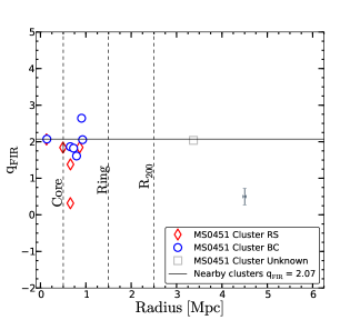
Figure 3: Plot of the galaxy projected radius against the far-IR to radio luminosity ratio $q_{\rm FIR}$. The mean value of $q_{\rm FIR}$ for low redshift cluster galaxies of Reddy & Yun (2004) is shown in the solid horizontal line ($q_{\rm FIR}$=2.07). Similar to Reddy & Yun (2004), the vertical dashed lines define the R_Core, R_Ring as the projected cluster-centric distance at R $\leq$ 0.5 and between [0.5, 1.5] Mpc, respectively. The error bars correspond to average 1$\upsigma$ errors.

In Figure 3, we plotted the far-IR and radio luminosity ratio ($q_{\rm FIR}$) as a function of the galaxy projected radius R in Mpc. In aiming to use radius as a proxy for local density, similar to Reddy & Yun (2004), we defined R_Core, R_Ring as the projected cluster-centric distance at R $\leq$ 0.5 Mpc and between [0.5, 1.5] Mpc, respectively. Miller & Owen (2001) and Reddy & Yun (2004) find a higher fraction of core galaxies that have a radio-excess, but we see no evidence of this in our sample drawn from one cluster.

Table 1: Properties of cluster galaxies that include the total IR luminosity (L_TIR) and rest frame radio luminosity (L_1.4GHz).

ID	RA	DEC	Redshift	$R$	S1.4	S1.4-err	log L1.4	S24	S24-err	log(L24μm)	log(L60μm)	log(LFIR)	log(LTIR)
	(Degree)	(Degree)		(Mpc)	($\upmu$Jy)	($\upmu$Jy)	(W Hz-1)	(mJy)	(mJy)	(L⊙)	(L⊙)	(L⊙)	(L⊙)
1081	73.514153	-2.988997	0.531	0.927	75.906	24.331	22.893	0.323	0.027	10.364	10.931	10.938	11.239
1093	73.521263	-2.994204	0.527	0.728	144.311	21.045	23.164	0.357	0.027	10.405	10.973	10.977	11.278
1118	73.518738	-3.003781	0.532	0.656	134.7	25.47	23.144	0.363	0.027	10.427	10.995	10.998	11.299
1143	73.516792	-2.990292	0.532	0.863	116.476	24.413	23.080	0.307	0.027	10.339	10.904	10.914	11.215
1158	73.520401	-3.000317	0.542	0.660	156.083	24.667	23.226	0.156	0.027	10.002	10.559	10.596	10.897
1178	73.523178	-2.988423	0.530	0.794	183.027	54.111	23.273	0.286	0.027	10.295	10.860	10.873	11.174
1489	73.534897	-3.054384	0.548	0.905	60.155	20.114	22.824	0.846	0.027	10.914	11.495	11.457	11.758
1726	73.549652	-3.044432	0.541	0.658	862.685	98.963	23.966	0.084	0.027	9.661	10.208	10.274	10.575
1811	73.550758	-3.016844	0.539	0.132	36.000	12.000	22.585	0.170	0.023	10.045	10.602	10.636	10.937
2143	73.558327	-3.033125	0.544	0.495	40.246	14.39	22.643	0.121	0.026	9.871	10.424	10.472	10.774
7240	73.551170	-3.016482	0.539	0.140	46.558	13.505	22.696	0.216	0.023	10.172	10.734	10.757	11.058
8110	73.396484	-3.020605	0.536	3.370	255.464	73.437	23.429	0.897	0.021	10.914	11.495	11.457	11.758

Table 2: Properties of field galaxies that include the total IR luminosity (L_TIR) and rest frame radio luminosity (L_1.4GHz).

ID	RA	DEC	Redshift	$R$	S1.4	S1.4-err	log L1.4	S24	S24-err	log(L24μm)	log(L60μm)	log(LFIR)	log(LTIR)
	(Degree)	(Degree)		(Mpc)	($\upmu$Jy)	($\upmu$Jy)	(W Hz-1)	(mJy)	(mJy)	(L⊙)	(L⊙)	(L⊙)	(L⊙)
1046	73.513374	-2.989720	0.578	0.930	1099.165	125.937	24.141	0.260	0.027	10.368	10.935	10.942	11.243
1743	73.547653	-3.042384	0.586	0.606	64.228	16.439	22.922	0.091	0.027	9.824	10.375	10.427	10.728
1937	73.550400	-3.057221	0.655	0.947	1530.335	260.189	24.414	0.314	0.027	10.621	11.195	11.181	11.482
2472	73.570877	-3.027037	0.617	0.639	307.426	28.24	23.654	0.359	0.026	10.622	11.196	11.182	11.483
2818	73.587166	-2.987284	0.239	1.153	114.59	31.547	22.273	0.317	0.029	9.299	9.836	9.931	10.232
2912	73.586548	-2.998683	0.725	1.018	79.373	25.822	23.233	0.193	0.030	10.475	11.044	11.043	11.344
3017	73.591164	-2.990986	0.489	1.187	109.072	34.843	22.967	0.110	0.036	9.664	10.211	10.276	10.577
3226	73.603012	-2.980324	0.725	1.541	656.767	39.495	24.150	0.198	0.040	10.491	11.060	11.058	11.359
3462	73.610458	-2.947674	0.728	2.141	220.184	38.439	23.680	0.172	0.039	10.418	10.986	10.989	11.290
3806	73.626404	-2.999176	0.332	1.883	210.369	38.786	22.860	1.336	0.034	10.461	11.030	11.030	11.331
3957	73.619141	-2.937129	0.323	2.450	192.012	58.31	22.795	1.741	0.032	10.562	11.134	11.125	11.426
5823	73.624580	-2.969661	0.447	2.084	153.757	41.791	23.023	0.472	0.033	10.326	10.891	10.902	11.203
6380	73.580307	-2.921304	0.619	2.286	245.952	45.472	23.561	0.453	0.013	10.750	11.327	11.302	11.603
6638	73.648750	-2.975052	0.447	2.526	390.0	50.734	23.427	0.834	0.021	10.625	11.199	11.185	11.486
7372	73.573524	-2.971213	0.777	1.199	113.395	31.084	23.460	0.149	0.027	10.415	10.982	10.986	11.287
8060	73.394081	-3.050711	0.491	3.513	213.045	73.092	23.261	0.074	0.022	9.450	9.992	10.074	10.375
8134	73.402657	-3.035359	0.715	3.258	312.974	74.698	23.814	0.329	0.023	10.753	11.330	11.306	11.607
8415	73.586739	-3.150578	0.505	3.199	224.847	63.553	23.313	0.240	0.013	10.138	10.699	10.725	11.026
8575	73.623688	-2.891933	0.900	3.326	2337.128	397.688	24.927	0.454	0.022	11.324	11.916	11.845	12.146
8578	73.655594	-2.971230	0.802	2.702	247.537	53.255	23.832	0.864	0.021	11.459	12.056	11.973	12.274
8581	73.659332	-2.969704	0.219	2.794	115.513	41.055	22.191	1.068	0.022	9.818	10.370	10.422	10.723
8583	73.648529	-2.962799	0.590	2.636	156.628	50.165	23.315	0.788	0.025	10.979	11.562	11.519	11.820
8608	73.670662	-2.991703	0.447	2.900	183.367	62.913	23.099	0.474	0.022	10.327	10.893	10.903	11.204
8631	73.664940	-3.052018	0.794	2.840	205.325	56.57	23.741	0.477	0.021	11.104	11.691	11.637	11.938
8642	73.693115	-3.053544	0.280	3.464	188.581	69.843	22.646	0.749	0.025	9.942	10.497	10.539	10.840
8773	73.578003	-2.830110	0.491	4.275	239.729	85.027	23.312	0.789	0.026	10.725	11.301	11.279	11.580
8813	73.656097	-2.904510	0.756	3.564	229.033	67.389	23.736	0.312	0.023	10.796	11.374	11.346	11.647

6.2 Potential Caveats

Before interpreting our findings, there are some caveats related to the derived luminosities which need to be considered.

6.2.1 Far-Infrared-Radio Relation: Presence of AGN

For comparison purposes and conformity to the previous work in the literature (Reddy & Yun, 2004), we do not a priori exclude AGN, but analyse both star-forming galaxies and AGN together. It has been established that faint radio populations are mostly found to be composed of star-forming galaxies and radio-quiet AGN (e.g. Jarvis & Rawlings, 2004). It is also acknowledged that there is generally a contribution to the net radio flux from an AGN which can affect the observed relationship. However, we do note that the optical spectra for our sources do not show evidence of AGN activity based on the lack of broad-line sources. We then followed the method of Stern et al. (2005) to check for AGN contamination using IRAC colour-colour plots which is shown in Figure 4. We particularly adopted the formulation in AB mag system by Messias et al. (2010) as shown in their Figure 4. We find no clusters sources that show any indication of being an AGN according to the classification as defined by Stern et al. (2005); Messias et al. (2010). The implications of AGN in our sample are further discussed in §7.

6.2.2 IR Luminosity Derived From 24 $\mu$m

Observations at 24 $\upmu$m may not be providing an unbiased estimator of the star formation since the peak of the IR SED tracing the cold dust component peaks between 60 $\upmu$m and 170 $\upmu$m (Pierini et al., 2003). Furthermore, 24 $\upmu$m data may be affected by dust heating from older stellar populations (Calzetti et al., 2010), although the 24 $\upmu$m flux is going to be dominated by the warm dust component.

In addition, there is an order a magnitude correction required to convert 24 $\upmu$m flux to total IR flux, which small scatter in the relationship can contribute large uncertainties. However, Dale et al. (2001) argued that 20-42 $\upmu$m is essentially a good tracer of the bulk of dust emission and hence can be a robust recent star formation indicator. Recent studies of the relationship in the field have also found consistent results between mid-infrared MIPS 24 $\upmu$m and MIPS 70 $\upmu$m results (e.g. Appleton et al., 2004; Beswick et al., 2008). In addition, Murphy et al. (2011) find that 24 $\upmu$m observations are a sufficient tracer of the total IR luminosity of galaxies for galaxies with L_24μm$<$10¹² L_⊙, which includes all of our cluster sample.

Galametz et al. (2013) combined Spitzer and Herschel data and noted that an inclusion of 24 $\upmu$m wavelength is essential in order to robustly derive the total IR luminosity for nearby star-forming galaxies. In addition, for luminous galaxies at z $<$ 1.3, measurement based on mid-IR is in agreement with those measured directly with Herschel, as already shown by Elbaz et al. (2011).

6.2.3 Small Sample Size

Given the fact that we have studied only one cluster containing a relatively small number of members, it is important to note that the current results may suffer from small sample size. In our sample, we did not detect the brightest cluster galaxy (which is obscured by a foreground galaxy) while Reddy & Yun (2004) have 4 cDs in their sample.

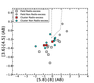
Figure 4: Plot of AGN indices. IRAC colour-colour diagnostic for AGN.

7 Discussions

Among the low redshift cluster studies, the far-infrared-radio relationship in rich cluster galaxies is characterised by a lower value of $q_{\rm FIR}$ as compared to the field that is indicative of an excess of radio emission. Cluster environmental effects are believed to drive these observations (Andersen & Owen, 1995; Rengarajan et al., 1997). Andersen & Owen (1995) postulated that the ISM of galaxies in rich clusters is being compressed via ram pressure as the galaxies move through the ICM resulting in greater radio emission. More recent work has further examined various models to shed some light on the causes of enhanced radio emission that seems globally present in cluster galaxies (Miller & Owen, 2001; Reddy & Yun, 2004; Murphy et al., 2009). The most common scenarios include thermal pressure compression by the ICM and the ram pressure stripping of ISM, which are both likely to augment the galactic magnetic field.

If we compare our results with the study of low redshift clusters by Reddy & Yun, 2004, we find the following: (1) the intermediate redshift cluster sample has a lower value of $q_{\rm FIR}$ = 1.80$\pm$0.15 with a dispersion of 0.53, but one that is consistent within the dispersion with the low redshift clusters where $q_{\rm FIR}$ = 2.07$\pm$0.07 with a dispersion of 0.74; (2) the fraction of radio-excess objects in clusters at intermediate redshifts is greater than in the low redshift ($27^{+23}_{-13}\%$ to $11\%$); (3) We find no preference for radio excess objects in the cluster core. However, we caution that any results from this work may suffer from the small sample size studied here.

Our measurement of $q_{\rm TIR}$ in the field at intermediate redshift is consistent with previous work (Murphy et al., 2009; Ivison et al., 2010a; Jarvis et al., 2010; Ivison et al., 2010b), and little or no evolution has been reported in the evolution of the $q_{\rm TIR}$ value in the field at these redshifts (e.g. Sargent et al., 2010a, b; Ivison et al., 2010b; Bourne et al., 2011). However, the significant increase in the scatter in the $q_{\rm FIR}$ value is inconsistent with these works as well as the scattered measured by Yun et al., 2001 at low redshift. The high scatter that we are measuring may be due to preferentially selecting radio bright objects especially at higher redshift. For this reason, we will focus on the observed fraction of radio-excess objects seen in the cluster and the behaviour of blue galaxies in the cluster.

In the intermediate redshift cluster, we observe a higher fraction of radio-excess galaxies as compared to lower redshift. Two thirds of the sources classified as radio-excess sources are red sequence galaxies. Reddy & Yun (2004) found that 9 of 13 excess sources at low redshift had AGN signatures and were early-type galaxies. From visual inspection of their spectra and analysis of their mid-infrared colours, our two red galaxies do not show broad emission lines or other telltale AGN signatures, but their large offset from the relationship may be indicative of nuclear activity. As can be seen in Figure 2, most of the blue galaxies appear normal and have a very small scatter in their $q_{\rm FIR}$ values. We find one blue galaxy showing a radio-excess.

In Figure 3, we do not see any strong radial trends against the $q_{\rm FIR}$ values. However, we notice that there is a significant scatter within the ring galaxies. Overall, inspection of the median $q_{\rm FIR}$ value indicates that the far-infrared-radio relation for cluster blue galaxies at $z$ $\sim$ 0.5 is similar to the cluster sample at low redshift.

At low redshift clusters, one interpretation of the presence of radio-excess within the virial radius can be the results of interstellar medium (ISM) stripped off via ram pressure exerted by infalling galaxies. We do not see any strong environmental effects in the value of $q_{\rm FIR}$ at these redshifts, although we do see a greater percentage of excess objects. It is possible that the quenching mechanism is different than it is at low redshift although a larger sample would be required to verify this. Follow-up observations of these excess objects found at intermediate redshift clusters would also help in exploring their properties.

However, we note the radio spectral index $\alpha$ depends on frequency and galaxy properties and thus using a single spectral index may also alter the value of $q$ (e.g. Bourne et al., 2011). However, the majority of work of this kind has been using the standard spectral index for normal star-forming galaxies; $\alpha$ $\sim$ 0.8 of Condon (1992). Recent results from the local infrared luminous galaxies of Murphy et al. (2013) found that the mid-infrared and radio properties of star-forming galaxies, particularly for those compact starburst galaxies, tend to have a flatter ($\alpha$ $\sim$ 0.5) spectral index. This may be a concern for galaxies in clusters as Crawford et al. (2006, 2011) find an increase in compact galaxies in clusters at these redshifts. The recently upgraded VLA correlator now makes it possible to measure the spectral index over a wide bandwidth within a single observation, so it will be a powerful tool for determining the IR-radio relation for large field and cluster samples in the future.

8 Conclusion

We have studied the far-infrared-radio relation in the massive galaxy cluster MS0451-03 and investigated, for the first time, how this relationship behaves at intermediate redshift between the field and a high-density cluster environment. We have constructed the far-infrared-radio relationship of star-forming galaxies using deep VLA and $Spitzer$ archival data. We have measured the rest frame radio luminosity at 1.4 GHz and the total IR luminosity ratios for both sample of confirmed MS0451-03 cluster and field galaxies.

We find that the far-infrared-radio relationship for distant cluster populations $(q_{\rm FIR}$ = 1.80$\pm$0.15 with a dispersion of 0.53) is in agreement with those measured in low redshift clusters ($q_{\rm FIR}$ = 2.07$\pm$0.07 with a dispersion of 0.74). We do find an evidence for a cluster enhancement of the radio excess sources with the value in MS0451-03 ($27^{+23}_{-13}\%$) being significantly higher than that in low redshift clusters ($11^{+1.7}_{-4.7}\%$). In addition, the far-infrared-radio relationship for blue galaxies, where $q_{\rm FIR}$ = 2.01$\pm$0.14 with a dispersion of 0.35, is consistent with the predicted value from the field relationship, although these results are based on a sample from a single cluster. We find one radio-excess galaxy among the blue star forming galaxies and two RS galaxies with radio-excess. Unlike low redshift galaxies, our galaxies do not show any evidence of AGN activity, but further observations will be needed to confirm the nature of these objects. We do not find any trends with radius for radio-excess populations within this one cluster.

In the future work, we will expand our sample of distant and rich clusters to further explore the relationship at intermediate redshift. The subsequent analysis of the extended sample shall provide higher statistics and will allow further confirmation of differences seen between low and intermediate redshift.

Appendix A Equations Used To Estimate IR Luminosities

Additional materials are provided in this Appendix which consists of empirical relations used to estimate IR luminosities and a table that contains various $q$-values in the literature (See Table 4).

A.1 IR Luminosities Inferred From Empirical Relations

A.1.1 Estimating total IR luminosity (L_TIR)

Measurement of IR luminosity can be made through an empirical relation via either a single IR band or a combination of many IR bands. The total IR luminosity for our sources was solely determined through the MIPS 24 $\upmu$m empirical relation.

Rieke et al. (2009) compute total IR luminosity (L_TIR) as described in Sanders et al. (2003); Sanders & Mirabel (1996). The luminosity estimator of Sanders & Mirabel (1996) is defined at $\lambda=8\mbox{--}1000\,\mu\mbox{m}$; L(TIR; 8–1000 $\upmu$m) and L_TIR is given by:

$$L_{\rm TIR}\ [L_{\odot}]\sim 4.93\times 10^{-22}(13.48{L}_{\nu}(12\mu\mbox{m})+5.16{L}_{\nu}(25\mu\mbox{m})$$

$$+2.58{L}_{\nu}(60\mu\mbox{m})+{L}_{\nu}(100\mu\mbox{m}))$$

where ${L}_{\nu}$ [$\mbox{erg\,s}^{-1}\mbox{Hz}^{-1}$] is defined as the luminosity per unit frequency at a frequency $\nu=c/\lambda$ where $c$ is the speed of light.

In this work, L_TIR was computed using the 24 $\upmu$m luminosity (L_24μm) via an empirical relation of Rieke et al. (2009); (see, Equation (A6) in Rieke et al., 2009), which is given by Equation 5.

$$\rm log\ L_{\rm TIR}=(1.445\pm 0.155)+(0.945\pm 0.016)\ log\ L_{24\rm\upmu m}$$ (5)

Furthermore, in order to be consistent throughout our calculations and comparisons, we also used other formulations of Rieke et al. (2009) to estimate the L_60μm and L_FIR. These transformations are presented in the next sections.

A.1.2 Inferring IR luminosity at 60 $\mu$m (L_60μm)

We computed the L_60μm using the following relation taken from Rieke et al. (2009); (see, Equation (A7) in Rieke et al., 2009), which is given by Equation 6.

$$\rm log(L_{\rm TIR})=(1.183\pm 0.101)+(0.920\pm 0.010)\ log(L_{60\rm\upmu m});$$

$$\rm Hence,\ log(L_{60\rm\upmu m})=\frac{log(L_{\rm TIR})-1.183}{0.920}$$ (6)

A.1.3 Inferring far-IR luminosity (L_FIR)

It is common to study the relationship between the IR and radio luminosity using the classical far-IR luminosity as defined by Helou et al. (1988) at $\lambda=42\mbox{--}122\,\mu\mbox{m}$. The far-IR luminosity L(FIR; 42–122 $\upmu$m) estimator is given by:

$$L_{\rm FIR}\ [L_{\odot}]\sim 3.29\times 10^{-22}\times\left(2.58{L}_{\nu}(60\mu\mbox{m})+{L}_{\nu}(100\mu\mbox{m})\right)$$

where ${L}_{\nu}$ [$\mbox{erg\,s}^{-1}\mbox{Hz}^{-1}$] is defined as the luminosity per unit frequency at a frequency $\nu=c/\lambda$ where $c$ is the speed of light.

In this work, we estimated the L_FIR based on the assumption that the global ratio of L_TIR, L(TIR; 8–1000 $\upmu$m), and L_FIR L(FIR; 42–122 $\upmu$m) luminosity is approximately 2 (see e.g., Bell, 2003), and see also in L_TIR defined as L(TIR; 3–1100 $\upmu$m) (see e.g., Dale et al., 2001; Dale & Helou, 2002). We have adopted the following relation as shown in Equation 7.

$$\rm L_{\rm TIR}/L_{\rm FIR}\sim 2;\ or\ L_{\rm FIR}\sim 0.5\times L_{\rm TIR}$$ (7)

Table 3: SFR(flux) fit coefficients A and B as a function of redshift for MIPS. $A(z)$ and $B(z)$ are to be used in Equation 2 and 3 as the intercept and slope of the relation of SFR on observed IR flux (see, Rieke et al., 2009).

$z$	$A_{24}$	$B_{24}$
0.0	0.417	1.032
0.2	0.502	1.169
0.4	0.528	1.272
0.6	0.573	1.270
0.8	0.445	1.381
1.0	0.358	1.565
1.2	0.505	1.745
1.4	0.623	1.845
1.6	0.391	1.716
1.8	0.072	1.642
2.0	0.013	1.639
2.2	0.029	1.646
2.4	0.053	1.684
2.6	0.162	1.738
2.8	0.281	1.768
3.0	0.371	1.782

Table 4: This table summarizes various range of the IR and radio luminosity ratios mean values found in the literature. A non-exhaustive list of paper is presented as per the following: reference, redshift, environment, value $q$₂₄, $q$_FIR and value of $q$_TIR along with the available either a dispersion or an error of the mean.

Reference	Redshift	Environment	Mean $q$24	Mean $q$FIR	Mean $q$TIR
This work	$\sim$0.54	Cluster	0.69$\pm$0.55	1.80$\pm$0.53; $\lambda$(42–122)	2.10$\pm$0.53; $\lambda$(8–1000)
Reddy & Yun (2004)	0.0120$<$z$<$0.025	Cluster	——–	2.07$\pm$0.74; $\lambda$(42–122)	——–
Yun et al. (2001)	$\leq$0.16	Field	——–	2.34$\pm$0.01; $\lambda$(42–122)	——–
Murphy et al. (2009)	$\sim$0.0036	Cluster	——–	2.10$\pm$0.25; $\lambda$(42–122)	——–
Rieke et al. (2009)	$\leq$0.088	Field	1.22$\pm$0.02	2.42$\pm$0.23; $\lambda$(42–122)	——–
Miller & Owen (2001)	0.016$<$z$<$0.033	Cluster	——–	2.30$\pm$0.20; $\lambda$(42–122)	——–
Andersen & Owen (1995)	$<<$0.2	Cluster	——–	2.27$\pm$0.20; $\lambda$(42–122)	——–
Younger et al. (2009)	1.5$<$z$<$3.0	Field	——–	2.23$\pm$0.04; $\lambda$(40–120)	——–
Sajina et al. (2008)	0.5$<$z$<$3.0	Field	——–	2.07$\pm$0.01; $\lambda$(40–120)	——–
Kovács et al. (2006)	1$<$z$<$3	Field	——–	2.07$\pm$0.09; $\lambda$(42–122)	——–
Garrett (2002)	$\leq$1.4	Field	——–	2.00; $\lambda$(40–120)	——–
Helou et al. (1985)	$\sim$0.0036	Field	——–	2.14$\pm$0.14; $\lambda$(42–122)	——–
Bourne et al. (2011)	0$<$z$<$2	Field	1.47$\pm$0.03	——–	2.66$\pm$0.12; $\lambda$(8–1000)
Sargent et al. (2010a)	0$<$z$<$5	Field	1.26$\pm$0.13	——–	2.57$\pm$0.13; $\lambda$(8–1000)
Sargent et al. (2010b)	0$<$z$<$2	Field	——–	——–	2.585$\pm$0.245; $\lambda$(8–1000)
Ivison et al. (2010a)	0$<$z$<$3	Field	——–	——–	2.41$\pm$0.20; $\lambda$(8–1000)
Ivison et al. (2010b)	0$<$z$<$2	Field	——–	——–	2.40$\pm$0.24; $\lambda$(8–1000)
Jarvis et al. (2010)	0$<$z$<$0.5	Field	——–	——–	2.40$\pm$0.12; $\lambda$(8–1000)
Murphy et al. (2009)	0.6$\leq$z$\leq$2.6	Field	——–	——–	2.41$\pm$0.30; $\lambda$(8–1000)
Bell (2003)	local	Field	——–	2.36$\pm$0.02; $\lambda$(42–122)	2.64$\pm$0.02; $\lambda$(8–1000)
Garn et al. (2009)	0$<$z$<$2	Field	0.92$\pm$0.10	——–	——–
Beswick et al. (2008)	0$<$z$<$1.2	Field	0.52$\pm$0.20	——–	——–
Ibar et al. (2008)	$\leq$3.5	Field	0.71$\pm$0.47	——–	——–
Boyle et al. (2007)	$\leq$2.15	Field	1.39$\pm$0.02	——–	——–
Murphy et al. (2006)	$\leq$0.002	Field	0.92$\pm$0.35	2.33$\pm$0.14; $\lambda$(42–122)	——–
Appleton et al. (2004)	$\leq$2	Field	0.94$\pm$0.23	——–	——–

References

- Andersen & Owen (1995) Andersen V., Owen F. N., 1995, AJ, 109, 1582
- Appleton et al. (2004) Appleton P. N., et al., 2004, ApJS, 154, 147
- Barger et al. (1996) Barger A. J., Aragon-Salamanca A., Ellis R. S., Couch W. J., Smail I., Sharples R. M., 1996, MNRAS, 279, 1
- Bell (2003) Bell E. F., 2003, ApJ, 586, 794
- Berciano Alba et al. (2010) Berciano Alba A., Koopmans L. V. E., Garrett M. A., Wucknitz O., Limousin M., 2010, A&A, 509, A54
- Best et al. (2002) Best P. N., van Dokkum P. G., Franx M., Röttgering H. J. A., 2002, MNRAS, 330, 17
- Beswick et al. (2008) Beswick R. J., Muxlow T. W. B., Thrall H., Richards A. M. S., Garrington S. T., 2008, MNRAS, 385, 1143
- Boselli & Gavazzi (2006) Boselli A., Gavazzi G., 2006, PASP, 118, 517
- Bourne et al. (2011) Bourne N., Dunne L., Ivison R. J., Maddox S. J., Dickinson M., Frayer D. T., 2011, MNRAS, 410, 1155
- Boyle et al. (2007) Boyle B. J., Cornwell T. J., Middelberg E., Norris R. P., Appleton P. N., Smail I., 2007, MNRAS, 376, 1182
- Butcher & Oemler (1984) Butcher H., Oemler Jr. A., 1984, ApJ, 285, 426
- Calzetti et al. (2010) Calzetti D., et al., 2010, ApJ, 714, 1256
- Condon (1992) Condon J. J., 1992, ARA&A, 30, 575
- Condon et al. (1991) Condon J. J., Anderson M. L., Helou G., 1991, ApJ, 376, 95
- Crawford et al. (2006) Crawford S. M., Bershady M. A., Glenn A. D., Hoessel J. G., 2006, ApJL, 636, L13
- Crawford et al. (2009) Crawford S. M., Bershady M. A., Hoessel J. G., 2009, ApJ, 690, 1158
- Crawford et al. (2014) Crawford S. M., Wirth G. D., Bershady M. A., 2014, ApJ, 786, 30
- Crawford et al. (2011) Crawford S. M., Wirth G. D., Bershady M. A., Hon K., 2011, ApJ, 741, 98
- Dale & Helou (2002) Dale D. A., Helou G., 2002, ApJ, 576, 159
- Dale et al. (2001) Dale D. A., Helou G., Contursi A., Silbermann N. A., Kolhatkar S., 2001, ApJ, 549, 215
- Elbaz et al. (2011) Elbaz D., et al., 2011, A&A, 533, A119
- Fadda et al. (1996) Fadda D., Girardi M., Giuricin G., Mardirossian F., Mezzetti M., 1996, ApJ, 473, 670
- Fazio et al. (2004) Fazio G. G., et al., 2004, ApJS, 154, 10
- Galametz et al. (2013) Galametz M., et al., 2013, MNRAS, 431, 1956
- Garn et al. (2009) Garn T., Green D. A., Riley J. M., Alexander P., 2009, MNRAS, 397, 1101
- Garrett (2002) Garrett M. A., 2002, A&A, 384, L19
- Gehrels (1986) Gehrels N., 1986, ApJ, 303, 336
- Greisen (2003) Greisen E. W., 2003, Information Handling in Astronomy - Historical Vistas, 285, 109
- Helou et al. (1988) Helou G., Khan I. R., Malek L., Boehmer L., 1988, ApJS, 68, 151
- Helou et al. (1985) Helou G., Soifer B. T., Rowan-Robinson M., 1985, ApJL, 298, L7
- Ibar et al. (2008) Ibar E., et al., 2008, MNRAS, 386, 953
- Ivison et al. (2010a) Ivison R. J., et al., 2010a, MNRAS, 402, 245
- Ivison et al. (2010b) Ivison R. J., et al., 2010b, A&A, 518, L31
- Jarvis & Rawlings (2004) Jarvis M. J., Rawlings S., 2004, NewAR, 48, 1173
- Jarvis et al. (2010) Jarvis M. J., et al., 2010, MNRAS, 409, 92
- Kovács et al. (2006) Kovács A., Chapman S. C., Dowell C. D., Blain A. W., Ivison R. J., Smail I., Phillips T. G., 2006, ApJ, 650, 592
- Lutz et al. (2011) Lutz D., et al., 2011, A&A, 532, A90
- Magnelli et al. (2013) Magnelli B., et al., 2013, A&A, 553, A132
- Makovoz & Marleau (2005) Makovoz D., Marleau F. R., 2005, PASP, 117, 1113
- Maraston (2005) Maraston C., 2005, MNRAS, 362, 799
- Martini et al. (2009) Martini P., Sivakoff G. R., Mulchaey J. S., 2009, ApJ, 701, 66
- Messias et al. (2010) Messias H., Afonso J., Hopkins A., Mobasher B., Dominici T., Alexander D. M., 2010, ApJ, 719, 790
- Miller & Owen (2001) Miller N. A., Owen F. N., 2001, AJ, 121, 1903
- Moran et al. (2007) Moran S. M., Ellis R. S., Treu T., Smith G. P., Rich R. M., Smail I., 2007, ApJ, 671, 1503
- Morrison et al. (2010) Morrison G. E., Owen F. N., Dickinson M., Ivison R. J., Ibar E., 2010, ApJS, 188, 178
- Morrison et al. (2003) Morrison G. E., Owen F. N., Ledlow M. J., Keel W. C., Hill J. M., Voges W., Herter T., 2003, ApJS, 146, 267
- Murphy (2009) Murphy E. J., 2009, ApJ, 706, 482
- Murphy et al. (2006) Murphy E. J., et al., 2006, ApJ, 638, 157
- Murphy et al. (2009) Murphy E. J., Chary R.-R., Alexander D. M., Dickinson M., Magnelli B., Morrison G., Pope A., Teplitz H. I., 2009, ApJ, 698, 1380
- Murphy et al. (2011) Murphy E. J., Chary R.-R., Dickinson M., Pope A., Frayer D. T., Lin L., 2011, ApJ, 732, 126
- Murphy et al. (2009) Murphy E. J., Kenney J. D. P., Helou G., Chung A., Howell J. H., 2009, ApJ, 694, 1435
- Murphy et al. (2013) Murphy E. J., Stierwalt S., Armus L., Condon J. J., Evans A. S., 2013, ApJ, 768, 2
- Noll et al. (2009) Noll S., Burgarella D., Giovannoli E., Buat V., Marcillac D., Muñoz-Mateos J. C., 2009, A&A, 507, 1793
- Oliver et al. (2012) Oliver S. J., et al., 2012, MNRAS, 424, 1614
- Owen & Morrison (2008) Owen F. N., Morrison G. E., 2008, AJ, 136, 1889
- Pierini et al. (2003) Pierini D., Popescu C. C., Tuffs R. J., Völk H. J., 2003, A&A, 409, 907
- Reddy & Yun (2004) Reddy N. A., Yun M. S., 2004, ApJ, 600, 695
- Rengarajan et al. (1997) Rengarajan T. N., Karnik A. D., Iyengar K. V. K., 1997, MNRAS, 290, 1
- Rieke et al. (2009) Rieke G. H., Alonso-Herrero A., Weiner B. J., Pérez-González P. G., Blaylock M., Donley J. L., Marcillac D., 2009, ApJ, 692, 556
- Rieke et al. (2004) Rieke G. H., et al., 2004, ApJS, 154, 25
- Saintonge et al. (2008) Saintonge A., Tran K.-V. H., Holden B. P., 2008, ApJL, 685, L113
- Sajina et al. (2008) Sajina A., et al., 2008, ApJ, 683, 659
- Sanders et al. (2003) Sanders D. B., Mazzarella J. M., Kim D.-C., Surace J. A., Soifer B. T., 2003, AJ, 126, 1607
- Sanders & Mirabel (1996) Sanders D. B., Mirabel I. F., 1996, ARA&A, 34, 749
- Sargent et al. (2010a) Sargent M. T., et al., 2010a, ApJS, 186, 341
- Sargent et al. (2010b) Sargent M. T., et al., 2010b, ApJL, 714, L190
- Smith et al. (2012) Smith A. J., et al., 2012, MNRAS, 419, 377
- Stern et al. (2005) Stern D., et al., 2005, ApJ, 631, 163
- van der Kruit (1971) van der Kruit P. C., 1971, A&A, 15, 110
- Wardlow et al. (2010) Wardlow J. L., et al., 2010, MNRAS, 401, 2299
- Wold et al. (2012) Wold I. G. B., Owen F. N., Wang W.-H., Barger A. J., Keenan R. C., 2012, ApJS, 202, 2
- Younger et al. (2009) Younger J. D., et al., 2009, MNRAS, 394, 1685
- Yun et al. (2001) Yun M. S., Reddy N. A., Condon J. J., 2001, ApJ, 554, 803