Simulating realistic disk galaxies with a novel sub-resolution ISM model

Abstract

We present results of cosmological simulations of disk galaxies carried out with the GADGET-3 TreePM+SPH code, where star formation and stellar feedback are described using our MUlti Phase Particle Integrator (MUPPI) model. This description is based on a simple multi-phase model of the interstellar medium at unresolved scales, where mass and energy flows among the components are explicitly followed by solving a system of ordinary differential equations. Thermal energy from SNe is injected into the local hot phase, so as to avoid that it is promptly radiated away. A kinetic feedback prescription generates the massive outflows needed to avoid the over-production of stars. We use two sets of zoomed-in initial conditions of isolated cosmological halos with masses $(2-3)\cdot 10^{12}$ M_⊙, both available at several resolution levels. In all cases we obtain spiral galaxies with small bulge-over-total stellar mass ratios ($B/T\sim 0.2$), extended stellar and gas disks, flat rotation curves and realistic values of stellar masses. Gas profiles are relatively flat, molecular gas is found to dominate at the centre of galaxies, with star formation rates following the observed Schmidt-Kennicutt relation. Stars kinematically belonging to the bulge form early, while disk stars show a clear inside-out formation pattern and mostly form after redshift $z=2$. However, the baryon conversion efficiencies in our simulations differ from the relation given by Moster et al. (2010) at a $3\sigma$ level, thus indicating that our stellar disks are still too massive for the Dark Matter halo in which they reside. Results are found to be remarkably stable against resolution. This further demonstrates the feasibility of carrying out simulations producing a realistic population of galaxies within representative cosmological volumes, at a relatively modest resolution.

1 Introduction

The study of galaxy formation in a cosmological framework represents since more than two decades a challenge for hydrodynamic simulations aimed at describing the evolution of cosmic structures. This is especially true when addressing the problem of formation of disk galaxies (e.g. Mayer et al., 2008, for a review; a short updated review of past and present efforts in this field is presented it in Section 2).

The recent history of numerical studies of the formation of galaxies demonstrated that the most crucial ingredient for a successful simulation of a disk-dominated galaxy is proper modelling of star formation and stellar feedback (hereafter SF&FB). This history can be schematically divided into three phases. In a first pioneeristic phase the simplest models of SF&FB, based on a Schmidt-like law for star formation and supernova (SN) feedback in the form of thermal energy resulted in a cooling catastrophe, with too many baryons condensing into galaxy and most angular momentum being lost. Galaxy disks, when present, were very compact and with exceedingly high rotation velocities. Kinetic feedback was found to improve the results by producing outflows and reducing overcooling.

During the first decade of 2000, much emphasis was given to the solution of the angular momentum problem. It was fully recognised that structure in the Inter-Stellar Medium (ISM) below the resolution limit achievable in cosmological simulations was crucial in determining the efficiency with which SN energy is able to heat the surrounding gas and produce massive outflows, in the form of fountains or prominent galaxy winds.

In this paper we will adopt a conservative definition of “sub-resolution physics”: every process that is not explicitly resolved in a simulation implementing only fundamental laws of physics is defined to be sub-resolution. We make no difference between models that combine in a simple way the resolved hydrodynamical properties of gas particles and models that provide an explicit treatment of the unresolved structure of the ISM. In this sense, any star-formation prescription is sub-resolution, since the formation of a single star is not explicitly resolved. This also applies to any form of energetic feedback, as long as individual SN blasts are not resolved since their free expansion phase (or as long as radiative transfer of light from massive stars is not tracked), and to chemical evolution of gas and stars.

Several approaches to model the sub-resolution behaviour of gas were proposed (see Section 2). These approaches provided significant improvements in the description of disk galaxy formation. In spite of these improvements, the Aquila comparison project showed that, when running many codes on the same set of initial conditions of an isolated “Milky Way” sized halo, no code was able to produce a completely realistic spiral galaxy with low bulge-over-total ($B/T$) stellar mass ratio and flat rotation curve. Moreover, different SF&FB prescriptions gave very different results.

A third phase is taking place at present: thanks to a careful tuning of models and the introduction of more refined forms of kinetic and “early” stellar feedback, several independent groups are now succeeding in better regulating overcooling and the loss of angular momentum. This was done by using several different approaches to SF&FB, that may be broadly grouped into two categories. One approach is based on reaching the highest numerical resolution affordable with the present generation of supercomputers, thus resolving higher gas densities and pushing the need of sub-resolution modelling from $\la$kpc toward $\la$10 pc scales. Other groups prefer to improve and refine their sub-resolution models so as to be able to work at resolutions in the range from $\sim$kpc to $\sim$100 pc. This latter approach mainly focuses on the modelling of feedback and, in some case, on refining the sub–resolution description of the ISM structure.

In this paper we follow the latter approach. In Murante et al. (2010) we proposed a model for SF&FB called MUlti Phase Particle Integrator (MUPPI). While being inspired to the analytic model of Monaco (2004a), it has several points of contact with the effective model of Springel & Hernquist (2003). In MUPPI, each gas particle eligible to host star formation is treated as a multi-phase portion of the ISM, made by cold and hot gas in thermal pressure equilibrium and a stellar reservoir. Mass and energy flows among the various phases are described by a suitable system of ordinary differential equations (ODE), and no assumption of self-regulation is made. For each gas particle, the system of ODE is solved at each time step, also taking into account the effect of the hydrodynamics. SN energy is distributed to the gas particles surrounding the star forming ones both in thermal and kinetic form.

In Murante et al. (2010) we tested a first version of MUPPI, which described primordial gas composition and thermal feedback only, on isolated galaxies and rotating halos. We showed that simulations naturally reproduce the Schmidt-Kennicutt relation, instead of imposing it in the model (see also Monaco et al., 2012), and the main properties of the ISM. In the absence of kinetic feedback, the model generated galactic fountains and weak galactic winds, but strong galactic outflows were absent. Our model was included in the Aquila comparison project Scannapieco et al. (2012), and shared virtues and weaknesses of several other SF&FB models tested in that paper.

In this work, we describe an updated version of MUPPI and test it on cosmological halos. We implemented a kinetic feedback scheme and included the description of chemical evolution developed by Tornatore et al. (2007a), with metal-dependent cooling described as in Wiersma et al. (2009). Here we present results of zoomed-in cosmological simulations of Milky-Way sized DM halos. We use two sets of initial conditions, one of which is the same used in the Aquila comparison project, at different numerical resolutions. As a main result, we will show that our simulations produce realistic, disk-dominated galaxies, with flat rotation curves, low galactic baryon fractions and low value of the bulge-to-total stellar mass ratio ($B/T$), in good agreement with the Tully-Fisher and the stellar mass - halo mass relations. Since we use one of the Aquarius halo, which has also been recently simulated by Aumer et al. (2013) and Marinacci et al. (2013), we can show how, two years after the “Aquila” comparison project, simulated galaxy properties from different groups, using different codes and SF&FB algorithms, agree now much better with each other. Finally, we demonstrate that our simulations shows very good convergence with resolution. In a companion paper (Goz et al. 2014) we will present an analysis of the properties of bars found in the simulations presented here, while a forthcoming paper (Monaco et al., in preparation) we will present a more detailed discussion of the implementation of SF&FB and the optimisation of the choice of the model parameters.

The plan of the paper is as follows. In Section 2 we provide an overview of the literature on cosmological simulations of disk galaxies. The numerical implementation of the updated MUPPI model is described in Section 3. The properties of the simulations presented in the paper are given in 4. Results are presented and commented in Section 5, including a discussion on the effect of resolution and on numerical convergence. Section 6 summarises the main conclusions of our analysis.

2 Overview of simulations of disk galaxy formation

In this section, we provide a concise review of the results presented in the literature concerning simulations of disk galaxies in a cosmological context. As mentioned in the Introduction, past attempts to simulate disk galaxies can be divided in three distinct phases.

2.1 Pioneeristic phase

Starting from a first generations of pioneering analyses (e.g. Evrard 1988; Hernquist 1989; Hernquist & Katz 1989; Barnes & Hernquist 1991; Hiotelis & Voglis 1991; Katz & Gunn 1991; Katz et al. 1992; Thomas & Couchman 1992; Cen & Ostriker 1993; Navarro & White 1994a; Steinmetz & Muller 1995; Mihos & Hernquist 1996; Walker et al. 1996; Navarro & Steinmetz 1997; Carraro et al. 1998; Steinmetz & Navarro 1999; Sommer-Larsen et al. 1999; Lia & Carraro 2000), simulating a realistic spiral galaxy in a cosmological DM halo has been recognised as a tough problem to solve. The basic reason for this is that radiative gas cooling at high redshift produces a runaway condensation in the central parts of newly forming Dark Matter (DM) halos, the so-called “cooling catastrophe” (Navarro & Benz 1991, Navarro & White 1994b). As a result, baryonic matter loses orbital angular momentum along with the central parts of the host DM haloes (see also D’Onghia et al., 2006), thereby producing by $z=0$ galaxies that are too concentrated, compact and rapidly spinning.

Early attempts to form realistic disk galaxies relied a simple prescription for forming stars within a hydrodynamical cosmological simulation (e.g. Steinmetz & Mueller 1994, Katz et al. 1996; hereafter “simple star formation model”). In this model, a dense cold gas particle forms stars at a rate depending on $\beta\rho_{g}/t_{dyn}$, the ratio between its density and dynamical time, times an efficiency $\beta$ that is a free parameter of the model. This is a three-dimensional relation analogous to the two-dimensional one of Schmidt and Kennicutt (Schmidt 1959,Kennicutt 1998), with the free parameter to be chosen so as to reproduce the observational relation, which is recovered when projecting gas density of a thin rotating disc.

In this scheme, some form of energetic feedback is needed to regulate star formation in galaxies. Since gas circulating inside a DM halo falls back to the galaxy in a few dynamical times, feedback must be violent enough to eject gas from the halos. The right amount of energy is required to allow a fraction of this expelled gas to fall back at low redshift. At the same time, this feedback needs not to be too violent when star formation takes place in galaxy discs, with a low velocity dispersion. Supernovae (SNe) were recognised as the most plausible candidates as a driver of such feedback. SNe can supply energy to surrounding gas particles in two different forms, kinetic and thermal. Whenever the internal structure of star-forming molecular clouds is not resolved, thermal energy feedback is not efficient. In fact, star formation takes place where gas reaches high density and, therefore, has short cooling time. As a consequence, energy given to the gas surrounding a star-forming region is promptly radiated away (see e.g. Katz et al. 1992). Kinetic energy is much more resilient to radiative losses, so an implementation of kinetic feedback can easily produce massive outflows (Navarro & Steinmetz, 2000). When some form of kinetic feedback was used, experiments succeeded in producing realistic disk galaxies, but failed to produce bulge-less late-type spirals (Abadi et al., 2003; Governato et al., 2004).

2.2 The importance of the ISM physics

Springel & Hernquist (2003) introduced a new, more refined model for describing the process of star formation (hereafter “effective model”). They treated gas particles eligible to form stars as a multi-phase medium, composed by a cold and a hot phase in thermal pressure equilibrium. The cold gas forms stars at a given efficiency. This model describes mass and energy flows between the phases with a system of ODE, with equilibrium solutions that depend on average density and pressure of the gas. These equilibrium solutions are used to predict the star formation rate of a given star-forming gas element. This effective model has the following features: (i) it assumes quiescent, self-regulated star formation; (ii) as a consequence, thermal energy from SNe only establishes the equilibrium temperature of the hot gas phase, and thus thermal feedback cannot drive massive outflows; (iii) a (three-dimensional) Schmidt-like relation is imposed, not obtained as a result of the model; (iv) kinetic feedback is implemented using a phenomenological prescription, that is added to the model; (v) in order to guarantee the onset of galactic winds, gas particles subject to kinetic feedback become non-collisional for some time, during which they do not interact with the surrounding gas.

This model aims at providing a realistic description of the physical properties of the ISM at scales well below the numerical resolution limit. Such physics is considered to be the cause of two phenomena, that are necessary ingredients for a successful description of observed late-type spirals: quenching of early star formation and expulsion of significant amount of gas mass from the high-redshift DM halos. Part of the expelled gas must fall back in DM halos at low redshifts, thus allowing late, quiescent, ongoing star formation. The inside-out growth of stellar disks is due to this mechanism.

The effective model by Springel & Hernquist (2003) was used by Robertson et al. (2004) to perform simulations of the formation of a disk galaxy, and by Nagamine et al. (2004) and Night et al. (2006) to study the formation of Lyman-break galaxies in cosmological volumes. Okamoto et al. (2005) used the same model to study various regimes of feedback for quiescent and starburst star formation, triggered by high gas densities or strong shocks. They claimed that the latter trigger leads to an improvement in the production of extended disks. While these numerical experiments provided an improvement in the description of galaxy formation in a cosmological context, they were still not able to produce a fully realistic late-time spiral galaxy. Apart from having too large bulge masses, the fraction of baryons in the resulting galaxies were still too high when compared to the observed relation between halo mass and stellar mass relation.

The implementation of kinetic feedback by Springel & Hernquist (2003), where a fraction of the SN energy budget is given to the outflow particle and wind velocity is assumed to be constant, is usually referred to as energy-driven kinetic feedback. As an alternative, Oppenheimer & Davé (2006) proposed an implementation of momentum-driven winds where, following Murray et al. (2005), the outflow is driven by radiation pressure of massive stars more than by SNe. In this model, the wind terminal velocity scales with the galaxy circular velocity, a behaviour supported by observations (e.g. Martin, 2005; Oppenheimer & Davé, 2006, and references therein). In the numerical implementation of momentum-driven outflows, square root of the gravitational potential or velocity dispersion of DM particles can be used as proxies of the galaxy circular velocity (e.g. Tescari et al., 2009; Okamoto et al., 2010; Oser et al., 2010; Tescari et al., 2011; Puchwein & Springel, 2013). Other variants of this models for galactic winds were presented by Choi & Nagamine (2011) and Barai et al. (2013), that also provided detailed comparisons of the prediction of different outflow models (see also Schaye et al., 2010a; Hirschmann et al., 2013b).

Governato et al. (2007) adopted a feedback model previously suggested by Gerritsen & Icke (1997) and Thacker & Couchman (2000). In this model SN thermal energy is assigned to the neighbouring gas particles; these particles are then not allowed to cool for a given amount of time, so as to mimic the effect of SNe blast waves. This prescription evolved into the blast-wave feedback recipe by Stinson et al. (2006). These authors claimed that, to successfully tackle the angular momentum problem in disk-galaxy formation, high numerical resolution is needed.

Booth et al. (2007) proposed a star formation model in which molecular clouds form through radiative cooling, and subsequently evolve ballistically and coagulate whenever colliding. SPH was used to describe the ambient hot gas, with the effect of thermal SNe feedback modelled using solutions of Sedov blasts. They called their model “sticky particles” and showed that it is able to reproduce a number of observed properties of the ISM in simulations of isolated disk galaxies. Kobayashi et al. (2007) adopted a simple SF model and pure thermal feedback, but included the effect of hypernovae, that release ten times the energy of a normal SN-II. They focused on studying the impact of hypernovae feedback on star formation history and enrichment of diffuse baryons, but did not provide results on the morphological properties of their simulated galaxies.

Schaye & Dalla Vecchia (2008) pointed out that, if gas in a galaxy disc obeys an effective equation of state, as in the effective model of Springel & Hernquist (2003), then it obeys a Schmidt-Kennicutt relation. Based on this, they argued that it is easy to control star formation without the need of making assumptions about the unresolved ISM. Dalla Vecchia & Schaye (2008) also suggested that outflowing gas particles should not be hydrodynamically decoupled, thus at variance with Springel & Hernquist 2003. These prescriptions were used to simulate cosmological volumes in the GIMIC (Crain et al., 2009) and in the OWLS (Schaye et al., 2010b) projects. Later on Dalla Vecchia & Schaye (2012) suggested that thermal energy should be distributed in a more selective way: imposing a minimum temperature at which each gas particle must be heated, cooling times become longer than the sound-crossing time, thereby allowing heated particles to expand and produce outflows before energy is radiated away.

Following Marri & White (2003), Scannapieco et al. (2009) revised the SPH scheme to prevent overcooling of a hot phase which is spatially coexisting with cold gas: in this prescription, the search of neighbours of a hot gas particle is limited to those particles whose entropy is within a given range of entropy. They used a simple star formation prescription: SN thermal energy distributed to hot gas is not immediately radiated away, because of its lower density. Cold gas particles cumulate SN energy until they can be promoted to become hot particles. They simulated eight DM halos taken from the Aquarius project (Springel et al., 2008), with a mass similar to that of the Milky Way halo. None of their simulated galaxies had a disk stellar mass larger than 20 per cent of the total stellar mass of the galaxy. However, they emphasised that the alignment of the angular momentum of gas accreting on the galaxy is quite important for the formation of stable disks.

Ceverino & Klypin (2009) studied the role of SNe feedback on the multiphase ISM by combining high resolution, small scale simulations of the ISM and cosmological simulations. Their simulations were based on the Adaptive-Mesh Refinement (AMR) ART code (Kravtsov et al., 1997). They first carried out parsec-scale simulations of portions of a disk galaxy, then used them to build a sub-resolution model for SF&FB  in cosmological simulations. As a result of their analysis, they claimed that very high resolution is needed in this approach, so that they had to stop their cosmological simulation at high redshift, $z=3$. Colín et al. (2010) also used the ART code to study the effect of varying the sub-resolution model parameters on simulated low-mass galaxy properties. They implemented a simple star formation model, but stopped the cooling of gas receiving energy from SNe. They found that galaxy properties are very sensitive to these parameters: even tuning them, they were not able to reproduce observed properties of low-mass galaxies.

Increasing resolution and using a high value for star formation density threshold in their blast-wave SN feedback model, Governato et al. (2010) succeeded in producing a bulgeless dwarf galaxy. This galaxy was analysed in detail by Brook et al. (2011) and Christensen et al. (2012). They also added a prescription to estimate the amount of molecular hydrogen formed in the simulation and linked the star formation to it. Christensen et al. (2014) studied, with the same prescription, the scaling laws of galactic bulges.

Stinson et al. (2010) simulated a set of nine galaxies, with halo masses ranging from $5\times 10^{11}$ to $2\times 10^{12}$ M_⊙, with blast-wave feedback but a lower density threshold for star formation. They successfully reproduced the Tully-Fisher relation, but reported that their simulated galaxies still are too centrally concentrated. Using a similar SF&FB scheme, Piontek & Steinmetz (2011) confirmed that this implementation of feedback is able to alleviate the angular momentum problem, while varying the numerical mass resolution over four order of magnitude does not impact on the angular momentum loss.

With the ERIS simulation, Guedes et al. (2011) successfully produced a Milky-Way-like galaxy, with an extended disk, a flat rotation curve and a $B/D$ ratio as low as $B/D=0.35$ in the i-band. They used the same SF&FB model of Stinson et al. (2006), and obtained this result by using very high numerical resolution and a high density threshold for star formation. Agertz et al. (2011) used the RAMSES Eulerian AMR code (Teyssier, 2002), with a simple star formation model. They also turned off cooling for gas receiving SNe energy. Using a low star formation efficiency, but also a low density threshold, they successfully reproduced several observed properties of Milky-Way like galaxies. However, their circular velocities usually show a large peak at small radii. This problem is alleviated in their simulations based on the lowest efficiency SF efficiency and lowest density. We note that their mass resolution was approximately four times worse than that of ERIS simulations. Sales et al. (2010) carried out simulations of cosmological volumes, instead of a zoom-in simulation of a single galaxy, and found that a high density threshold for SF is required to produce realistic disks.

Another direction of investigation concerns the description of other sources of energy feedback, in addition to SNe. The effect of Active Galactic Nuclei (AGN) feedback is usually considered not to be very important in the formation of disk galaxies. However, it was included by some groups (Di Matteo et al. 2003, Springel et al. 2005, Booth & Schaye 2009, Hirschmann et al. 2013a). Besides SNe and AGN, cosmic ray pressure could also represent an important and known source of feedback, that can help in driving massive galaxy winds. Attempts to implement cosmic rays feedback in cosmological simulations were presented, e.g., by Jubelgas et al. (2008), Wadepuhl & Springel (2011) and Uhlig et al. (2012). The latter two works focused on the relevance of cosmic rays feedback for satellite and small galaxies.

2.3 Towards realistic disk galaxy simulations

While progress was achieved in the ability to produce disk galaxies, no consensus still emerged neither on the nature of feedback required, nor on the details of its numerical implementation. In the “Aquila comparison project”, Scannapieco et al. (2012) presented a comparison among 12 different Lagrangian and Eulerian codes implementing different SF&FB prescriptions. An earlier version of MUPPI, not including chemical evolution and kinetic feedback, also took part of this comparison project. Nine of such models were implemented in the same TreePM+SPH code GADGET-3 (non-public evolution of the code GADGET-2, Springel et al. 2005). The conclusion of the comparison was that better agreement with observations, both in terms of fraction of halo mass in the galaxy and in terms of conservation of angular momentum, was obtained with SF&FB models that have more effective feedback. As a general result, all the simulated galaxies tended to be too massive, too compact and centrally concentrated. Also, the models that are most successful in producing a flat rotation curve had to resort to such a strong feedback that the disk component was destroyed or very thick. The results were presented at two different resolutions, and the numerical convergence was generally not particularly good. To cite the conclusion of the paper by Scannapieco et al. (2012) : “state-of-the-art simulations cannot yet uniquely predict the properties of the baryonic component of a galaxy, even when the assembly history of its host halo is fully specified.”

This work triggered a burst of efforts to improve the different models in the direction of resolving the discrepancies with observations.

Stinson et al. (2013a) used the same SF&FB model of Crain et al. (2009) and showed that, in their cosmological run, many disk galaxies with flat rotation curves and low baryon fractions were present, even if their resolution was low ($M_{DM}\approx 7\cdot 10^{7}$ M_⊙). Their model was included in the Aquila comparison project, and indeed their results were among the best, although with rather peaked rotation curves.

At smaller halo masses, Stinson et al. (2013b) obtained a realistic late-type galaxy, with a moderate mass resolution (mass of the dark matter particle $m_{DM}=1.1\times 10^{6}$ M_⊙) and using the simple SF model and the blastwave feedback. In this work they introduced a form of “early stellar feedback”, motivated by the expectation that the UV radiation of young stars can quench the star formation rate in cold molecular clouds. This concept was already introduced by Hopkins et al. (2011); the difference is that while Hopkins et al. (2011) used isolated idealised galaxy model, that allowed them to reach high resolutions and directly model the kinetic radiation pressure from young stars, Stinson et al. (2013b) modelled the same process as thermal feedback.

Aumer et al. (2013) simulated a subset of the halos from the Aquarius project, using an improved version of the model by Scannapieco et al. (2009). They added a non-decoupled kinetic feedback, along with feedback from radiation pressure of young massive stars, that was already experimented in Hopkins et al. (2011). Also their results improved considerably over those reported by the Aquila comparison project. With the above prescriptions, their model is able to produce realistic late-type spiral galaxies.

Vogelsberger et al. (2013) used the moving-mesh hydro code AREPO (Springel, 2010), with a modified version of the effective model. They performed cosmological simulations with various prescriptions of kinetic feedback; in one of them, the wind speed depends on the mass of the host DM halo, in line with Oppenheimer & Davé (2006) and Puchwein & Springel (2013). Their simulations included also AGN radiation feedback, i.e. the possibility of AGN radiation to destroy molecular clouds. They successfully matched a number of observational properties of the galaxy population, such as the Tully-Fisher relation and the stellar mass-halo mass relation. Unfortunately they did not discuss galaxy morphologies.

Marinacci et al. (2013) used AREPO and the same sub-resolution model of Vogelsberger et al. (2013) to simulated again the Aquarius set of initial conditions. Also in this case, they produced realistic late-type galaxies, with low $B/T$ ratios and low baryon fractions. To obtain this result they scaled their kinetic feedback with halo mass, similarly to the momentum-driven wind mechanism explained above, but increasing by a factor of three the standard value of $10^{51}$ erg associated to each SN explosion.

Hopkins et al. (2013) presented a series of simulations of individual galaxies, spanning a wide range of halo masses. They employed high resolution (up to $\approx 2.4\times 10^{4}$ M_⊙ in cosmological runs, for the DM particles), a simple SF model with a high density threshold ($n_{h}=100$ cm^-3), early stellar feedback both in the form of radiation pressure and photo-ionisation of molecular clouds. SN feedback was implemented as energy- or momentum-driven, depending on whether the shock of the supernova bubble is energy- or momentum- conserving at the resolved scales. They were able to achieve such high densities thanks to an extremely small gravitational softening length for baryonic particles. They predicted a relation between stellar mass and halo mass in good agreement with observational results, but provided no information on the morphology of galaxies.

Vogelsberger et al. (2014a) presented a large, well resolved cosmological simulation, dubbed “Illustris”, performed using the same SF&FB of Vogelsberger et al. (2013). The box size is 106.5 Mpc ($h=0.704$), simulated at several resolutions. At their highest resolution, the DM particle mass is $1.26\cdot 10^{6}$ M_⊙. The galaxy population was analyzed in Vogelsberger et al. (2014b), Genel et al. (2014) and Vogelsberger et al. (2014c). Several properties of simulated galaxies agree well with observations, including the morphological classifications and the shape of late-type galaxy rotation curves. Some residual tensions remain between their simulation results and low-redshift observations, e.g. in the TF relation, the baryon convertion efficiency relation, and the stellar mass function; Vogelsberger et al. (2014b) point out that some other properties, namely colours of intermediate-mass galaxies and age of dwarf ones, are still not in agreement with observations.

Cen (2014) studied the colour bi-modality of galaxies at low redshift ($z=0.62$) using a large cosmological simulation named “LAOZI”. They used the Eulerian AMR code ENZO (Bryan & Norman, 2000; Joung et al., 2009) with a simple star formation prescription. They took into account the amount of UV photons produced by young stars, with SN kinetic energy assigned to the 27 cells centred around the exploding star. Also in this case, no detailed morphological analysis of simulated galaxies was carried out.

Schaye et al. (2014) presented a suite of cosmological simulations, named “EAGLE”. The included sub-resolution physics is that described in Schaye et al. (2010b). Their larger simulation has a size of $100$ Mpc ($h=0.68$), a mass resolution of $9.7\cdot 10^{6}$ M_⊙ and a force resolution of $0.7$ kpc. They paid particular attention to the calibration of sub-resolution model parameters. These simulations reproduce a number of observational properties of galaxies, in particular the stellar mass function, though the authors state that gas and stellar metallicities of their dwarf galaxies are still too high.

In summary, different groups claim at present to be able to produce late-type spiral galaxies with properties similar to the observed ones. In general, some consensus emerges as for the need to significantly heat up or kick gas at early times through galactic winds, and to have efficient feedback to form disk galaxies (see Übler et al. (2014) for a recent work on this subject). On the other hand, no consensus has been reached on the source of the required feedback energy: are SNe alone sufficient to provide this energy, or do we need early stellar radiation, or AGN feedback, or cosmic ray feedback, or a combination of them? Moreover, a number of open questions, concerning technical points, have been raised and not yet fully solved. Is extremely high numerical resolution mandatory to simulate realistic disk galaxies? Do we need models with a high density threshold for the star forming gas? Is there a unique combination of threshold and star formation efficiency that allows us to simulate realistic disk galaxies? How important is the choice of hydrodynamic scheme on which simulations are based?

In the following, we present cosmological simulations of individual disk galaxies, carried out with GADGET3 including our sub-resolution model MUPPI. Our model describes the behaviour of the ISM at unresolved scales, but does not include early stellar feedback, high density threshold for star formation and AGN feedback. We will show that with this prescription we obtain late-type galaxies with properties in broad agreement with observation without the need of reaching extremely high resolution. A comparison with results from other groups, that simulated one of the halos we present here, shows that simulation results are quite close to each other, even if SF&FB models and hydro schemes are significantly different. In this sense, our results further demonstrate that possible avenues exist to produce realistic disk galaxies, relying on a relatively low resolution that can be afforded in large-scale simulations of representative volumes of the universe.

3 The sub-resolution model

In this Section, we describe the updated implementation of the MUPPI algorithm for star formation and stellar feedback. MUPPI is implemented within the TreePM+SPH GADGET3 code, which represents an evolution of the TreePM+SPH GADGET2 (Springel, 2005). Our version of GADGET-3 includes a uniform UV background from Haardt & Madau (2001), chemical evolution, metal cooling and kinetic feedback. A brief account of the original version of the algorithm, described in full detail in Murante et al. (2010), is given in Section 3.1, while the changes introduced in this work, in particular chemical evolution, metal cooling and kinetic feedback, are described in Sections 3.2 and 3.3.

3.1 The MUPPI algorithm

We assume that our simulations work at a typical force resolution in the range from 100 pc to 1 kpc, and at a mass resolution from from $10^{4}$ to $10^{7}$ M_⊙. In these conditions, the ISM of a star-forming region will have much structure at unresolved scales. The aim of our sub-grid model is to provide a description of this multi-phase gas which is accurate enough to represent in a realistic way the emergent effects of star formation and stellar feedback on resolved scales.

Following Monaco (2004b), we assume that each SPH particle that is eligible to host star formation (under a set of conditions that will be specified below) represents a multi-phase ISM that is composed by a hot, tenuous and pervasive gas phase and a cold phase that is fragmented into clouds with a low filling factor. These two phases are assumed to be in pressure equilibrium. A fraction of the cold phase, that we call molecular gas fraction, provides the reservoir for star formation. Spawning of collisionless star particles from the resulting stellar component of star-forming particles takes place according to a standard stochastic star formation algorithm (Katz et al., 1992; Springel & Hernquist, 2003). The hot phase is heated by the emerging energy from massive and dying stars and radiatively cools.

This setting is quantified as follows. Within each SPH particle of mass $M_{\rm P}$, the masses of the hot, cold and stellar components are $M_{\rm h}$, $M_{\rm c}$ and $M_{\star}$. If $n_{\rm h}$ and $n_{\rm c}$ are the particle number densities of the two gas phases, and $T_{\rm h}$ and $T_{\rm c}$ their respective temperatures, the condition of pressure equilibrium translates into:

$$n_{\rm h}\cdot T_{\rm h}=n_{\rm c}\cdot T_{\rm c}\,.$$ (1)

Here $T_{\rm c}$ should be considered as an effective temperature, that also takes into account the effect of kinetic pressure; this is left as a free parameter in the model.

Densities of cold and hot phases are computed starting from their filling factors: calling $F_{\rm h}$ the fraction of gas mass in the hot phase (the cold phase having a mass fraction of $F_{\rm c}=1-F_{\rm h}$), its filling factor $f_{\rm h}$ is:

$$f_{\rm h}=1-f_{\rm c}=\frac{1}{1+\frac{F_{\rm c}}{F_{\rm h}}\cdot\frac{\mu_{\rm h}}{\mu_{\rm c}}\cdot\frac{T_{\rm c}}{T_{\rm h}}}\,.$$ (2)

Then, if $\rho$ is the average gas density, for the two phases we have

$$n_{\rm h,c}=\rho F_{\rm h,c}/f_{\rm h,c}\mu_{\rm h,c}m_{p}\,,$$ (3)

$\mu_{h,c}$ being the corresponding molecular weights.

The molecular fraction is computed using the phenomenological relation by Blitz & Rosolowsky (2006) between the ratio of surface densities of molecular and atomic gas, and the estimated external pressure exerted on molecular clouds. Using the hydrodynamic pressure of the particle in place of the external pressure, we obtain a simple way to estimate the molecular fraction $f_{\rm mol}$:

$$f_{\rm mol}=\frac{1}{1+P_{0}/P}$$ (4)

A gas particle enters the multi-phase regime whenever its temperature drops below $10^{5}$ K and its density is higher than a threshold value $\rho_{\rm thr}$. The multi-phase system is initialised with all the mass in the “hot” component, $M_{\rm h}=M_{\rm P}$ and $T_{\rm h}=T_{\rm P}$, where $T_{\rm P}$ is the gas temperature. Its evolution is described by a system of four ordinary differential equations (see below), in which the variables are the masses of the three components, $M_{\rm h}$, $M_{\rm c}$ and $M_{\star}$, and the thermal energy of the hot phase $E_{\rm h}$. At each SPH time-step, this system is integrated with a Runge-Kutta integrator with adaptive time-steps. This means that the integration time-step is much shorter than the SPH one. To mimic the disruption of molecular clouds due to the activity of massive stars, and to limit the entrainment of the cold phase in a particle dominated (in volume) by the hot phase, a multi-phase cycle lasts at most a time $t_{\rm clock}$, that is set to be proportional to the dynamical time of the cold phase, $t_{\rm dyn}$; this quantity is defined below and used to compute the star formation rate. A particle exits the multi-phase regime also when its density becomes lower that $1/5$ of the entrance density threshold $\rho_{\rm th}$. Moreover, at low densities it can happen that the energy from SNe is not sufficient to sustain a hot phase. This results in a hot phase temperature that does not raise above $10^{5}$ K but remains very low. In this case the particle is forced to exit the multi-phase regime. A particle that has exited the multi-phase regime can enter it at the next time-step, if it meets the required conditions.

Matter flows among the three components as follows: cooling deposits hot gas into the cold phase; evaporation brings cold gas back to the hot phase; star formation moves mass from the cold gas to the stellar component; restoration moves mass from stars back to the hot phase. This is represented through the following system of differential equations:

$$\dot{M}_{\star} = \dot{M}_{\rm sf}-\dot{M}_{\rm re}$$ (5)

$$\dot{M}_{\rm c} = \dot{M}_{\rm cool}-\dot{M}_{\rm sf}-\dot{M}_{\rm ev}$$ (6)

$$\dot{M}_{\rm h} = -\dot{M}_{\rm cool}+\dot{M}_{\rm re}+\dot{M}_{\rm ev}$$ (7)

The various terms of the system (5-7) are computed as follows. The cooling flow $\dot{M}_{\rm cool}$ is

$$\dot{M}_{\rm cool}=\frac{M_{\rm h}}{t_{\rm cool}}\,.$$ (8)

This implies that cooling leads to the deposition of mass in the cold phase, at constant $T_{\rm h}$, and not to a decrease of $T_{\rm h}$. The cooling time is computed using hot phase density and temperature, $n_{\rm h}$ and $T_{\rm h}$, so that cooling times are relatively long whenever the hot phase has a low mass fraction and a high filling factor. The star formation rate is

$$\dot{M}_{\rm sf}=f_{\star}\cdot\frac{f_{\rm mol}\cdot M_{\rm c}}{t_{\rm dyn}}\,,$$ (9)

where the dynamical time of the cold gas phase is given by

$$t_{\rm dyn}=\sqrt{\frac{3\pi}{32G\rho_{\rm c}}}\ {\rm yr}\,.$$ (10)

As explained and commented in Murante et al. (2010), during each multi-phase cycle the dynamical time is computed as soon as 90 per cent of mass is accumulated in the cold phase, and is left constant for the rest of the cycle. Following Monaco (2004b), evaporation is assumed to be proportional to the star formation rate:

$$\dot{M}_{\rm ev}=f_{\rm ev}\cdot\dot{M}_{\rm sf}$$ (11)

In the absence of chemical evolution, the restoration term $\dot{M}_{\rm re}$ is computed in the Instantaneous Recycling Approximation (IRA):

$$\dot{M}_{\rm re}=f_{\rm re}\cdot\dot{M}_{\rm sf}\,,$$ (12)

otherwise the modelling of this mass (and metal) flow is performed by the chemical evolution code, as described in the next Section.

The fourth variable of the model is the thermal energy of the hot phase, $E_{\rm h}$. Its evolution is described as

$$\dot{E}_{\rm h}=\dot{E}_{\rm heat,local}-\dot{E}_{\rm cool}+\dot{E}_{\rm hydro}$$ (13)

The first heating term reads

$$\dot{E}_{\rm heat,local}=E_{\rm SN}\cdot f_{\rm fb,local}\cdot\frac{\dot{M}_{\rm sf}}{M_{\rm\star,SN}}\,.$$ (14)

and accounts for the contribution of SN energy from stars formed in the same multi-phase particle. Here $E_{\rm SN}$ is the energy supplied by a single supernova, and $M_{\rm\star,SN}$ the stellar mass associated to each SN event, while $f_{\rm fb,local}$ is the fraction of SN energy that is deposited in the hot phase of the particle itself. Consistently with the mass cooling flow, energy losses by cooling are expressed as

$$\dot{E}_{\rm cool}=\frac{E_{\rm h}}{t_{\rm cool}}\,.$$ (15)

The $\dot{E}_{\rm hydro}$ term takes into account the energy due to interactions with the neighbour particles. It is computed as the energy accumulated during the last hydrodynamical timestep, divided by the timestep itself. This energy accounts for the change in entropy given by SPH hydrodynamics, i.e. the $PdV$ work on the particle plus the effect of numerical viscosity, and for the SN energy coming from neighbouring particles.

Apart from the small fraction $f_{\rm fb,local}$ given to the star-forming particle itself, the energy budget from SNe is distributed in the form of thermal and kinetic energy. The thermal energy distributed to neighbours by each star-forming particle can be written as

$$\Delta E_{\rm heat,o}=E_{\rm SN}\cdot f_{\rm fb,out}\cdot\frac{\Delta M_{\star}}{M_{\rm\star,SN}}\,.$$ (16)

To mimic the blow-out of superbubbles along the least Resistance path (see Monaco, 2004b), each multi-phase particle distributes its thermal energy to particles that are within its SPH smoothing length and lie within a cone whose axis is aligned along the direction of minus the local density gradient, and whose semi-aperture angle is $\theta$. Energy contributions are weighted with the SPH kernel, but using the distance from the cone axis in place of the radial distance. This thermal feedback scheme is relatively effective even at high densities. In fact cooling has the effect of depositing hot gas into the cold phase, and cooling times are computed using density and temperature of the hot phase, so they are relatively long. The main effect of cooling is then to reduce the mass fraction of hot gas, while its temperature is kept high by SN feedback; when the particle is taken in isolation ($\dot{E}_{\rm hydro}=0$), energy injection from SNe and the relation between pressure and molecular fraction (Equation 4) create a runaway of star formation, until the molecular fraction saturates to unity. The particle can lower its pressure by expanding and performing $PdV$ work on other particles. Therefore, it is the hydrodynamic interaction with neighbouring particles that halts the runaway. This non-equilibrium dynamics is strong enough to avoid the formation of very cold and dense blobs. However, the effectiveness of thermal feedback is more limited when the contribution from metal lines is included.

At the end of the integration, we use the new state of the multi-phase system to recompute the entropy of the gas particle; the entropy change will thus include the effect of thermal energy from SNe. The entropy determines the internal energy and pressure of the particle, so this change will be self-consistently accounted for by the SPH hydrodynamical integrator.

As mentioned above, the creation of star particles is implemented with the stochastic algorithm described by Springel & Hernquist (2003). The probability of a gas particle to spawn a new star particle is proportional to the (virtual) stellar mass formed during the last hydrodynamical time-step. When a star particle is spawned, its mass is taken from $M_{\star}$; if this is not sufficient, the remaining mass is taken from the cold phase, or from the hot phase in the unlikely case the mass is still insufficient.

In summary, the parameters of the model are $T_{\rm c}$, $P_{0}$, $f_{\rm re}$ (when chemical evolution is not implemented), $f_{\rm ev}$, $f_{\star}$, $t_{\rm clock}$, $\rho_{\rm thr}$, $\theta$ and the energy fractions $f_{\rm fb,local}$ and $f_{\rm fb,out}$. Their values are given and commented in Murante et al. (2010), and have been slightly adjusted to the newest version including chemical evolution, taking values as reported in Table 1. As a remark on the density threshold $\rho_{\rm thr}$, we remind that it should not be confused with the star formation density threshold used, e.g., in the effective model of Springel & Hernquist (2003). In our model a gas particle can be in the multi-phase regime, but have very low star formation rate; this happens when the molecular fraction is low, due to low pressure. For example, if we consider the “star formation threshold” as the value of the numerical density of the cold phase where $f_{mol}=1/2$, taking reference values of $P_{0}/k_{B}=20000$ K cm^-3, $T_{c}=300$ K, in Eq. (4) we have $n_{c}T_{c}=P_{0}/k_{B}$, from which the threshold would be $n_{c}=66.6$ cm^-3. This high density is however modelled at the sub-resolution level, without the need of resolving it.

Table 1: Parameters of MUPPI. Column 1: Cold phase temperature (K). Column 2: Pressure at which $f_{\rm mol}=0.5$ (K cm^-3). Column 3: restoration fraction (now computed by the chemical evolution model). Column 4: evaporation fraction. Column 5: star formation efficiency (referred to the molecular gas). Column 6: duration of a multi-phase cycle in dynamical times. Column 7: density threshold for multi-phase particles (cm^-3). Column 8: Semi-aperture of the cone (degrees). Column 9: SN thermal energy given to local hot gas. Column 10: SN thermal energy given to neighbouring hot gas. Column 11: SN kinetic energy given to wind particles. Column 12: Probability for a gas particle to be converted in a wind particle. Parameters marked with $\star$ have been revised with respect to what reported by Murante et al. (2010).

$T_{\rm c}$	$P_{\rm 0}$	$f_{\rm re}$	$f_{\rm ev}$	$f_{\star}$	$t_{\rm clock}/t_{\rm dyn}$	$rho_{\rm thr}$	$\theta$	$f_{\rm fb,local}$	$f_{\rm fb.out}$	$f_{\rm fb,kin}$	$P_{\rm kin}$
300⋆	20000⋆	—⋆	0.1	0.02	1⋆	0.01	60	0.02	0.2⋆	0.6⋆	0.03⋆

3.2 Chemical evolution, metal cooling

We have merged MUPPI with the chemical evolution code originally presented by Tornatore et al. (2007b). In this code each star particle is treated as a Simple Stellar Population (SSP), whose evolution is followed starting from the time at which it has been spawned from a gas particle. Given a stellar Initial Mass Function (IMF), the mass of the SSP is varied in time following the death of stars, and accounting for stellar mass losses. We follow the production of several elements through SNII, SNIa and AGB stars. The enriched material is spread among the neighbouring gas particles with weights given by the SPH kernel. For each gas particle the code tracks the mass in $H$, $He$ and in several other chemical species, namely $C$, $Ca$, $O$, $N$, $Ne$, $Mg$, $S$, $Si$, $Fe$, plus that in generic other elements. When a star particle is spawned, its composition is taken as the one of the parent gas particle.

The code allows us to flexibly choose the stellar Initial Mass Function (IMF), the minimum stellar mass for SNII, metal yields, stellar lifetimes, and the elements to follow in detail. In this paper, stellar lifetimes are taken from Padovani & Matteucci (1993), we assume the IMF proposed by Kroupa et al. (1993), in the range 0.1-100 M$\odot$. This IMF is similar to that proposed by Chabrier (2003) ​in the same range. SNII are assumed to be originated by stars more massive than 8 M_⊙, while stars more massive than 40 M_⊙ are assumed to implode into black holes and not to contribute to chemical enrichment. Metal yields are taken from Woosley & Weaver (1995) for SNII, Thielemann et al. (2003) for SNIa and van den Hoek & Groenewegen (1997) for AGB stars. We follow the production of ten metal species, namely $C$, $Ca$, $O$, $N$, $Ne$, $Mg$, $S$, $Si$, $Fe$, plus $He$.

The implementation of the chemical evolution model by Tornatore et al. (2007b) follows the injection of energy from SNe along with mass ejection. In its integration with MUPPI we have decoupled the treatment of energy and mass. Energy injection is treated by MUPPI in the IRA as explained above, while the energy from SNIa is not implemented in the present version of the code. Mass restoration from dying stars is not treated in the IRA, as in Equation 12; the same mass flow $\dot{M}_{\rm re}$ is used to inject into the hot phase, at each SPH time-step, the mass (including metals) acquired from nearby star particles during the previous time-step. Because this mass is connected to dying stars, we assume that the energy necessary to keep it hot comes from the SN thermal energy budget. Finally, the parameter $M_{\rm\star,SN}$ is computed from the assumed IMF as the inverse of the number of stars more massive than 8 M_⊙ per unit mass of stars formed.

The contribution of metals to gas cooling is computed by following the procedure of Wiersma et al. (2009) (as in Planelles et al., 2013; Barai et al., 2013). The emissivity of an optically thin gas of a specified composition, under the influence of a uniform ionising background (from Haardt & Madau, 2001) is computed without assuming fixed (solar) abundance ratios of elements or collisional ionisation equilibrium.

3.3 Kinetic feedback

The original version of our SF&FB model included SN feedback only in the form of thermal energy. As illustrated in Monaco et al. (in prep), thermal feedback alone is able to efficiently suppress star formation when cooling is included for a gas of primordial compositions, although at the cost of creating a very hot circum-galactic halo. On the other hand, the efficiency of thermal feedback is much weaker when metal cooling is included, and much overcooling takes place. The reason for this is that thermal feedback can trigger fountain-like outflows of $\sim 50$ km s^-1, so that suppression of star formation for a Hubble time is obtained not by ejecting gas from the halo but by keeping it hot. This is no longer possible when cooling is boosted by a factor of 10 or more due to the higher metallicity. On the other hand, SNe inject both thermal and kinetic energy in the ISM, so it is natural to expect an emergence of energy at the $\sim$kpc scale both in thermal and in kinetic form.

To implement a kinetic feedback scheme, we broadly follow the scheme by Springel & Hernquist (2003), but with several differences to make it compatible with the thermal feedback scheme. When a particle exits a multi-phase cycle, we assign it a probability $P_{\rm kin}$ to become a “wind” particle. For some time $t_{\rm wind}$, such particles can receive kinetic energy from neighbouring multi-phase particles. Because outflows are driven by SNII exploding after the destruction of the molecular cloud, this time is set equal to the stellar lifetime of an 8 M_⊙ star, $t_{8}$, minus the duration $t_{\rm clock}$ of the past multi-phase cycle:

$$t_{\rm wind}=t_{8}-t_{\rm clock}\,.$$ (17)

However, the wind phase stops earlier than $t_{\rm wind}$ whenever the particle achieves low density, set to $0.3\rho_{\rm thr}$. For each star-forming particle, the available kinetic energy budget is

$$E_{\rm kin}=f_{\rm fb,kin}E_{\rm SN}\,.$$ (18)

This energy is distributed from multi-phase particles to wind particles with the same scheme of thermal energy: eligible wind particles are those within the SPH kernel and within a cone of semi-aperture $\theta$, anti-aligned with the density gradient, with relative contribution weighted by the distance from the cone axis. These particles receive “velocity kicks” as follows. For each wind particle we compute the energy contributions from all kicking particles and the energy-weighted average vector from kicking particles to the wind one. Then the kinetic energy of the wind particle is increased and the increase in velocity is in the direction defined above. The emergence of the wind, presumably due to the blow-out of an SN-driven super-bubble, takes place at scales that are still smaller than the ones that are typically resolved. Therefore, in order to avoid hydrodynamical coupling at $\sim$kpc scale, the wind particle is decoupled from the surrounding gas as long as it receives kinetic energy. However, we have verified that, when the hydrodynamical decoupling is not implemented, the resulting galaxy has very similar properties compared to the one obtained with decoupled winds; gas discs are slightly more perturbed, but this perturbation does not propagate into an appreciable thickening of the stellar disc.

In our prescription, the free parameters are $P_{\rm kin}$ and $f_{\rm fb,kin}$. Our tests suggest for them the values of 0.03 and 0.6, respectively, as specified in Table 1. At variance with other kinetic wind prescriptions, neither wind mass-load nor wind velocity are fixed. Nevertheless, typical values of these quantities can be estimated as follows. In a time interval $\Delta t$, the gas mass that will be uploaded in wind reads

$$\Delta M_{\rm wind}=P_{\rm kin}N_{\rm gas}\frac{\Delta t}{\langle t_{\rm dyn}\rangle}{\langle m_{\rm gas}\rangle}\,,$$ (19)

where$M_{\rm gas}$ is the mass of gas in multi-phase in a given region, $N_{\rm gas}=M_{\rm gas}/{\langle m_{\rm gas}\rangle}$ is the total number of multi-phase gas particles within the same region, $\langle t_{\rm dyn}\rangle$ the average dynamical time of the cold phase, and $\langle m_{\rm gas}\rangle$ the average gas particle mass (our particle have can have variable mass). The mass load can then be cast in the form

$$\dot{M}_{\rm wind}=P_{\rm kin}{1\over<t_{\rm dyn}>}N_{\rm gas}<m_{\rm gas}>=P_{\rm kin}\frac{M_{\rm gas}}{<t_{\rm dyn}>}$$ (20)

As such, it depends on the cold phase density, and then on pressure through $\langle t_{\rm dyn}\rangle$. Since in one time step, using Eq. 9, we have

$$\Delta M_{*}=f_{\rm cold}f_{\rm mol}f_{*}{M_{\rm gas}\over\langle t_{\rm dyn}\rangle}\Delta t$$ (21)

where we defined $f_{\rm cold}=M_{c}/M_{\rm gas}$, from the definition of mass load factor $\eta=\dot{M_{\rm wind}}/\dot{M_{\rm sfr}}$ we obtain

$$\eta={P_{\rm kin}\over f_{\rm cold}f_{\rm mol}f_{*}}$$ (22)

With our choice of parameters, we obtain $\eta\simeq 1.5$.

Conversely, the mass-weighted average wind velocity at the end of the wind phase is

$$<v_{\rm wind}>=2(\frac{<e_{\rm kin}>}{P_{\rm kin}M_{\rm gas}})^{1/2}\,,$$ (23)

where $e_{\rm kin}$ is the mass-weighted kinetic energy deposited in the gas mass $M_{\rm gas}$ in one dynamical time. Similarly, defining $v_{\rm SN}^{2}=E_{\rm SN}/M_{*,SN}$ it is easy to show that

$$v^{2}_{\rm wind}={f_{\rm fb,kin}\over\eta}v_{\rm SN}^{2}$$ (24)

With the chosen parameters, we obtain $v^{2}_{\rm wind}\simeq 600$ km s^-1. Note that, since these values depend on $\langle t_{\rm dyn}\rangle$, that varies depending on the local gas properties, the exact values of the mass load and wind velocity will also depend on such local properties. We will present a detailed analysis of our feedback model in a forthcoming paper (Monaco et. al., in preparation).

4 Simulations

In this work, we simulated two sets of cosmological zoomed-in halos. The standard zoom-in technique consists in isolating the object of interest in a low resolution, usually DM only simulation, at redshift $z=0$. Particles are then traced back to their Lagrangian coordinates. The region occupied by these particles, the “Lagrangian” region of the forming halo, is then resampled at higher resolution and with the addition of gas particles, taking care of conserving both amplitudes and phases of the original Fourier-space linear density. The refined Lagrangian region is chosen to include, at the final redshift, a volume that is larger than the virial radius of the selected halo, in order to avoid that lower-resolution particles affect the evolution of the halo. The resolution is degraded at larger and larger distances from the Lagrangian region of interest. This technique allows to greatly increase the resolution in the chosen halo, while correctly describing the effect of the large-scale tidal field. As a side note, we remark that the evolution of a resimulated object changes when resolution is varied: in fact, power added at small scales modifies the halo’s accretion history, e.g. the timing of the mergers and the distribution of the angular momentum.

The two sets of initial conditions describe the evolution of two isolated halos with mass in the range $\sim(1-2)\cdot 10^{12}$ $h^{-1}$ M_⊙, both having a quiet merging history since $z\sim 2$. Due to the lack of recent major mergers, these halos are expected to host an $M_{*}$ disk galaxy at $z=0$. In both cases initial conditions are available at several resolutions. The first set of initial conditions, called GA in this paper, has been presented in Stoehr et al. (2002). The second set, called AqC in this paper, has been presented by Springel et al. (2008) and used, among other papers, in the Aquila comparison project (Scannapieco et al., 2012). We refer to the original papers for more details on the construction of the two sets of initial conditions.

We used three different resolutions for the GA set and two for the AqC set. Table 2 shows mass and force resolutions used for our simulations, together with the virial mass and radius . Virial masses and radii are quite stable against resolution; there is a slight increase in virial mass in the GA set, going from our intermediate to our highest resolution. Our chosen ICs span a factor of 87 in mass for the GA set and a factor of 8 for the AqC set. Force softening was chosen to be constant in physical coordinates since $z=6$, while it is comoving with Hubble expansion at higher redshift. We scaled the softening of the GA set with the cubic root of the mass resolution. For the AqC5 and AqC6 simulations we used the same softenings as for GA2 and GA1, respectively.

For comparison, our highest mass resolution is the same used by Marinacci et al. (2013) and Aumer et al. (2013) for the AqC5 halo. Our intermediate mass resolution is a factor $\approx 5$ better than the resolution used by Vogelsberger et al. (2013). Comparing with the Eris simulation presented in Guedes et al. (2011), resolution in the GA2 and AqC5 simulations are coarser by a factor 21.4 in mass and by a factor 3.9 in gravitational softening.

The GA set used a $\Lambda$CDM cosmology with $\Omega_{m}=0.3$,$\Omega_{\Lambda}=0.7$, $\Omega_{baryon}=0.043$ and $H_{0}=70$ km s^-1. Also AqC was run with a $\Lambda$CDM cosmology, but with $\Omega_{m}=0.25$,$\Omega_{\Lambda}=0.75$, $\Omega_{baryon}=0.04$ and $H_{0}=73$ km s^-1.

Table 2: Basic characteristics of the different runs Column 1: simulation name; Column 2: mass of the DM particles; Column 3: initial mass of the gas particles; Column 4: Plummer-equivalent softening length for gravitational force. Column 5: Virial mass of the DM halo at $z=0$; Column 6: Virial radius of the DM halo at $z=0$; Column 7: number of DM particles within the virial radius at $z=0$; Column 8: number of gas particles within the virial radius at $z=0$; Column 9: number of star particles within the virial radius at $z=0$; Masses are expressed in units of h^-1M_⊙ and softening lengths in units of h^-1 kpc.

Simulation	$M_{\rm DM}$	$M_{\rm gas}$	$\epsilon_{\rm Pl}$	$M_{\rm Vir}$	$R_{\rm Vir}$	$N_{\rm DM}$	$N_{\rm gas}$	$N_{\rm star}$
GA0	$1.4\cdot 10^{8}$	$2.6\cdot 10^{7}$	1.4	$2.28\cdot 10^{12}$	212.72	13998	5873	24021
GA1	$1.5\cdot 10^{7}$	$2.8\cdot 10^{6}$	0.65	$2.30\cdot 10^{12}$	212.56	133066	68130	178626
GA2	$1.6\cdot 10^{6}$	$3.0\cdot 10^{5}$	0.325	$2.20\cdot 10^{12}$	209.89	1214958	534567	1429204
AqC6	$1.3\cdot 10^{7}$	$4.8\cdot 10^{6}$	0.65	$1.21\cdot 10^{12}$	169.03	87933	40362	123307
AqC5	$1.6\cdot 10^{6}$	$3.0\cdot 10^{5}$	0.325	$1.16\cdot 10^{12}$	166.75	687003	276881	898777

5 Results

In this Section, we first present results obtained from the highest resolution GA2 and AqC5 halos at $z=0$. The evolution of galaxies with redshift is discussed in Section 5.3, while the effect of resolution is presented in Section 5.4.

5.1 Galaxy Morphology

In Figure 1, we show face-on and edge-on maps of gas and stellar density for the GA2 simulation. We rotate the coordinate system so that its z-axis is aligned with the vector of angular momentum of star and cold or multi-phase gas particles within 8 kpc from the position of the minimum of the gravitational potential, and centered on it. This is the reference system with respect to which all of our analyses have been performed. The presence of an extended disk is evident in both gas and stellar components. The gas disk shows a complex spiral pattern and is warped in the outer regions. A spiral pattern is visible also in the outer part of the stellar disk. At the centre, a bar is visible both in the gas and in the stellar component. A full analysis of the bar features in our simulated galaxies is presented in the companion paper by Goz et al. (2014).The absence of a prominent bulge is already clear at a first glance of the stellar maps.

In Figure 2 we show the same maps for the simulation AqC5. The appearance of the galaxy is similar to that of GA2, though here the disk is smaller, the warp in the gas disk is less evident and the distribution of stars shows even clearer spiral pattern and bar.

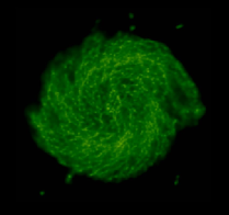
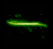
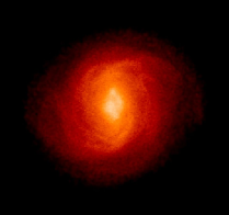
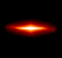
Figure 1: Projected gas (upper panels) and stellar (lower panels) density for the GA2 simulation. The z-axis of the coordinate system is aligned with the angular momentum vector of gas and stars enclosed within 8 kpc from the position of the minimum of the gravitational potential. Left panels show face-on densities, right column shows edge-on densities. Box size is $57$ kpc.

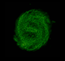
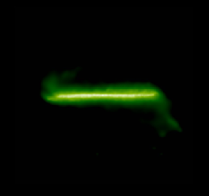
Figure 2: The same as in Fig. 1, but for the AqC5 simulation. Box size is $57$ kpc.

To quantify the kinematics of a galaxy it is customary to consider the distribution of orbit circularities of the star particles. The circularity $\epsilon$ of an orbit is defined as the ratio of the specific angular momentum in the direction perpendicular to the disk, on the specific angular momentum of a reference circular orbit: $\epsilon=J_{z}/J_{\rm circ}$. Scannapieco et al. (2009) computed the latter quantity as $J_{\rm circ}=r\cdot v_{c}(r)=r\sqrt{(}GM(<r)/r),$ where r is the distance of each star from the centre and $v_{c}(r)$ the circular velocity at that position. Abadi et al. (2003) instead define $J_{\rm circ}=J(E)$, where $J(E)$ is the maximum specific angular momentum allowed given the specific binding energy $E$ of each star; in this way $\epsilon<1.$

In Figure 3, we show the histograms of circularities of all star particles within $R_{\rm vir}/10$ for our GA2 and AqC5 simulations, using both methods outlined above.

We will use the second method in the rest of the present work, but show the results for both of them in this Figure to facilitate comparison with other works in literature that use the first one. The visual impression given by Figures 1 and 2 is confirmed by these distributions: at redshift $z=0$ both histograms show a prominent peak at $\epsilon\sim 1$, where stars rotating on a disk are expected to lie. The bulge component, corresponding to the peak at $\epsilon\sim 0$, is quite small in both cases, somewhat larger for GA2 than for AqC5. We estimate $B/T$, the ratio of bulge over stellar mass within $R_{\rm gal}$, by simply counting the counter-rotating stars and doubling their mass, under the hypothesis that the bulge is supported by velocity dispersion and thus has an equal amount of co- and counter-rotating stars. This kinematical condition selects both halo and bulge stars. Since our definition is based on the sign of the quantity $J_{z}/J_{\rm circ}$, it does not depend on the method used to evaluate the circularity distributions. The resulting ratios are $B/T=0.20$ for GA2 and $B/T=0.23$ for AqC5. As a matter of fact, Scannapieco et al. (2010) analysed a synthetic image of a simulated spiral galaxy with standard data analysis tools and showed that the definition of $B/T$ based on all counter-rotating stars overestimates what would be measured by an observer.

Even if the peak at $\epsilon\sim 0$ is higher for GA2, the total counter-rotating stellar mass is larger for AqC5. This is due to the larger stellar halo component of GA2, also visible in Figure 1.

In Figure 4, we show the rotation curves of GA2 and AqC5 at redshift $z=0$. We show the total rotation curve, and the contribution of DM, gas and stars separately for both simulations. Both galaxies have a remarkably flat rotation curve, reaching their maxima at 11.3 (AqC5) and 11.7 (GA2) kpc, after which they gently decline. The maximum rotation velocities are 270 and 299 km/s respectively, about 20 per cent higher than their circular velocities at the virial radius (and, incidentally, 20 per cent higher than the rotation velocity of the Milky Way at the solar radius, consistent with e.g. Papastergis et al. 2011).

From the visual appearance, from the shape of the rotation curves and from the distribution of circularities, it is clear that both simulated galaxies are disk-like and with a modest central mass concentration. This finding is at variance with respect to our earlier results published within the Aquila Comparison project (Scannapieco et al., 2012). The inclusion of metal-dependent gas cooling and, more important, the inclusion of kinetic feedback are the reason for this improvement.

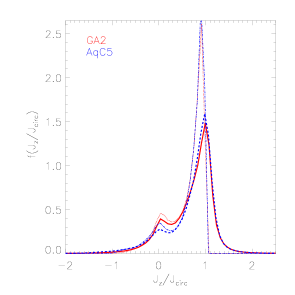
Figure 3: Distribution $f(\epsilon)/d\epsilon$ of the circularity parameter for the GA2 (red continuous and dotted lines) and AqC5 (blue dashed and dash-dotted lines) simulations at $z=0$, for the stellar component, as a function of the circularity $\epsilon=J_{z}/J_{\rm circ}$. Thick (continuous and dashed) lines show circularity evaluated as in Scannapieco et al (2009). Dotted and dash-dotted thin lines, as in Abadi et al. (2003). Distributions are normalized so that $\int f(\epsilon)d\epsilon=1$

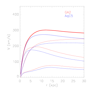
Figure 4: Rotation curves for the GA2 (red) and AqC5 (blue) simulations. Thick lines show the total curve, thin dashed lines show the contribution of the DM, thin dotted lines that of the gas, and thin dotted-dashed lines that of the stellar component.

Table 3: Basic characteristics of the different runs, done with MUPPI-std. Column 1: Simulation name; Column 2: Galaxy radius (kpc), set to $1/10$ of the virial radius; Column 3: Disk scale radius $R_{d}$ (kpc), obtained using and exponential fit fo the surface density profile of stars (See Figure 7) ; Column 4: B/T ratio inside the galaxy radius; Column 5: mass fraction associated to stars having circularity $\epsilon>0.8$ ; $\epsilon$ is calculated using the method of Scannapieco et al (2009), while we report in parenthesis the values obtained using the method by Abadi et al. (2003); Column 6: Total galaxy stellar mass, inside the galaxy radius (M_⊙); Column 7: Stellar mass in the bulge component inside the galaxy radius (M_⊙); Column 8: Stellar mass in the disk component inside the galaxy radius (M_⊙); Column 9: Stellar mass within the virial radius (M_⊙); Column 10: Cold gas mass (M_⊙); Column 11: Baryon fraction within virial radius; Column 12: Fraction of total baryon mass in the galaxy; Column 13: Ratio between the specific angular momentum of stars and cold gas within the galaxy radius and the specific angular momentum of the dark matter within the virial radius. The virial radius is defined as the radius of a sphere centered on the most bound particle of the halo, and encompassing and overdensity $\delta=200$ with respect to the critical density. The bulge mass is defined as twice the mass of counter-rotating stars, those having $j_{z}/j_{\rm circ}<0$ in Figure 3 and within 5 kpc from the galaxy center.

Simulation	$R_{\rm gal}$	$R_{d}$	$B/T$	$f(\epsilon>0.8)$	$M_{\star}$	$M_{\rm*,bulge}$	$M_{\rm*,disk}$	$M_{\rm*,vir}$	$M_{\rm cold}$	$f_{\rm b,vir}$	$f_{gal}$	$f_{J}$
GA0	30.39	1.98	0.30	0.24 (0.30)	$1.78\cdot 10^{11}$	$5.37\cdot 10^{10}$	$1.25\cdot 10^{11}$	$2.11\cdot 10^{11}$	$7.17\cdot 10^{9}$	0.13	0.06	0.28
GA1	30.37	3.93	0.22	0.47 (0.30)	$1.35\cdot 10^{11}$	$2.91\cdot 10^{10}$	$1.06\cdot 10^{11}$	$1.59\cdot 10^{11}$	$1.95\cdot 10^{11}$	0.11	0.049	0.56
GA2	29.98	4.45	0.20	0.51 (0.45)	$1.11\cdot 10^{11}$	$2.26\cdot 10^{10}$	$8.83\cdot 10^{10}$	$1.31\cdot 10^{11}$	$3.49\cdot 10^{10}$	0.10	0.043	0.54
AQ-C-6	24.15	4.08	0.24	0.51 (0.46)	$8.26\cdot 10^{10}$	$2.01\cdot 10^{10}$	$6.25\cdot 10^{10}$	$0.85\cdot 10^{11}$	$1.97\cdot 10^{9}$	0.11	0.057	1.18
AQ-C-5	23.82	3.42	0.23	0.55 (0.54)	$7.32\cdot 10^{10}$	$1.67\cdot 10^{10}$	$5.66\cdot 10^{10}$	$0.77\cdot 10^{11}$	$2.04\cdot 10^{10}$	0.10	0.054	0.92

In Table 3, we list the main characteristics of the simulated galaxies at $z=0$. Here the disk scale radius $R_{d}$ is estimated by fitting an exponential profiles to the stellar surface density from 4 to 12 kpc. Stellar masses are reported within $R_{\rm gal}=R_{\rm Vir}/10$, while cold gas includes multi-phase gas particles and single-phase ones with temperature lower than $10^{5}$ K. We also report the ratio of specific angular momenta of baryons in the disk (stars and cold gas) over that of the DM within the virial radius. We use all stars and cold gas within our galactic radius to evaluate such a ratio. This is a rough way to estimate the amount of loss of angular momentum suffered by “galaxy” particles: in case of perfect conservation, we would expect the specific angular momentum of these particles (condensed in the central region within $R_{\rm gal}$) to be the same as that of the dark matter halo (within $R_{\rm vir}$), so a value near unity is a sign of modest loss of angular momentum. Because we include all stars in the computation, we do expect to find some angular momentum loss. From Table 3, we note the following characteristics:

• Both halos host massive disk galaxies. The total stellar mass in the GA2 simulation is $1.02\cdot 10^{11}$ M_⊙, while it is $M_{\star}=6.77\cdot 10^{10}$ M_⊙ for AqC5. As such, and as also witnessed by their circular velocities, these galaxies are more massive than the Milky Way.

• The cold gas mass, that is assumed to be in the disk, is 28 per cent (GA2) and 26 per cent (AqC5) of the total disk mass, a value which is higher by a factor $2-3$ than for the Milky Way.

• Our feedback scheme is efficient in expelling baryons from the halo. For GA2, the baryon fraction within the virial radius is 10 per cent, compared to the cosmic 14.3 per cent, while the baryon mass of the galaxy (stars and cold gas) is 4.3 per cent of the total halo mass. These values are not far from those estimated for disk galaxies like the Milky Way. For AqC5 the baryon fraction within the virial radius is again 10 per cent, compared to the cosmic value of 16 per cent, and the fraction of galaxy mass to total mass is 5.4 per cent.

• The specific angular momentum of galactic baryons (cold gas and stars) in GA2 is 54 per cent of the specific angular momentum of the DM within the virial radius. In the AqC5 simulation, this fraction exceeds 1. This shows that in our simulations, baryons in the galaxy retain a fair share of their initial angular momentum. Thanks to our feedback scheme, we are thus able to prevent an excessive angular momentum loss, thereby allowing the formation of extended gaseous and stellar disks.

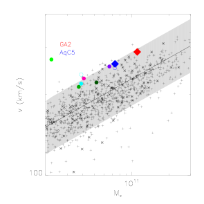
Figure 5: Tully-Fisher relation for our two simulated galaxies, GA2 (red diamond) and AqC5 (blue diamond). Galaxy mass is the stellar mass inside $R_{\rm gal}$; velocities are estimated from the circular velocity profile at $2.2R_{d}$. The line is the fit to observations of disk galaxies done by Dutton et al.(2011). The grey area shows an interval of 0.1 dex around the fit. Plus symbols are data points from Courteau et al. (2007), diamonds from Verheijen (2001) and asterixes from Pizagno et al. (2007). We also show for reference the position in the plot of AqC5 from Marinacci et al. (2013), where we took $V$ as the circular velocity at 2.2 times their quoted disk radius from their Figure 18 (purple circle); and the position of ERIS simulation, using their quoted $V_{\rm peak}$ (open cyan circle) and the circular velocity at 2.2 times their quoted i-band disk scale lenght, from their Figure 1 (filled cyan circle). The magenta circle shows the position of AqC5 simulated by Aumer et al. (courtesy of M. Aumer and C. Scannapieco). Green filled circles show the position in the diagram of AqC5 simulations G3-TO, G3-CS and R-AGN from Scannapieco et al. 2012 (light green: G3-CS; medium green: G3-TO; dark green: R-AGN). For these, circular velocity is evaluated at the radius containing half of the galaxy stellar mass; blue empty circle refer to our AqC5 simulations, when using the same definition of circular velocity.

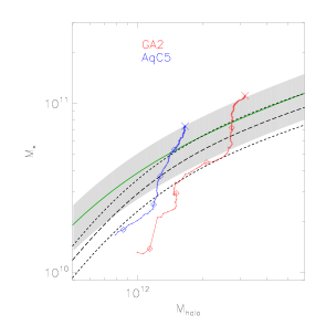
Figure 6: Evolution of the relation between stellar mass and halo mass ratio of GA2 (red) and AqC5 (blue). Crosses correspond to results at $z=0$, with the lines (with plus signs) showing the corresponding evolutions. Diamonds show redshifts $z=2$,$1.5$,$1.0$,$0.5$. The continuous green line shows the fit to the star formation efficiency of DM halos obtained by Guo et al. (2010) with the abundance matching technique. The grey area is an interval of 0.2 dex around it. The dashed black lines is the same fit, as given by Moster et al. (2010), while the dotted lines show an interval of 1$\sigma$ on the normalisation of the fit.

Figures 5 and 6 show the stellar Tully-Fisher relation and the stellar mass vs halo mass relation for our two simulations. Galaxy mass is the stellar mass inside $R_{\rm gal}$; velocities are taken from the circular velocity profile, at $2.2R_{d}$. As for the Tully-Fisher relation, we also plot the fit to observations of disk galaxies presented Dutton et al. (2011); in grey, we plot an interval $\pm 0.1$ dex around the fit for reference, and we overplot observations from Verheijen (2001),Pizagno et al. (2007) and Courteau et al. (2007). Symbols represent the position of our simulated galaxies in the plot. As in Dutton et al. (2011) we used the circular velocity at 2.2 times the disk radius of our galaxies (see Table 3).

For reference we also show the position in the same plot of AqC5 simulated by Marinacci et al. (2013), by Guedes et al. (2011) and by Aumer et al. (2013). We also show the position of three among the AqC5 simulations performed in Scannapieco et al. (2012), namely models G3-TO, G3-CS and R-AGN. Both our simulated galaxies tend to lie on the high side of the range allowed by observational results. We note that this is a common trend in recent simulated disk galaxies. This could be related to some remaining limitations shared in all SF&FB models used, or to the way in which simulations are compared to observations. Our simulated AqC5 galaxy has a stellar mass in good agreement with the finding of Marinacci et al. (2013), but higher than that found by other groups. In Table 3, we report the mass fraction of stars having a circularity larger than $\epsilon=0.8$; this quantity can be considered as a rough estimate of the prominence of the “thin” disk. Our higher resolution runs have fractions $f=0.51$ for GA2 and $f=0.55$ for AqC5, showing that the disk component of our simulations is significantly more important than that of most runs showed in the Aquila comparison project, and similar to that reported e.g. by Aumer et al. (2013), $f(\epsilon)=0.55$. On the other hand, our low-redshift SFR, shown in Figure 12, lies on the high side of the values shown e.g. in Aumer et al. (2013) for the same halo mass range. This suggests that the stellar mass excess we found could be due to late-time gas infall and its conversion in stars. Taken together, these data suggests that, with the parameter values used in this paper, our feedback scheme could be still slightly inefficient, either in quenching star formation at low redshift, or in expelling a sufficient amount of gas from haloes at higher redshift. But we have not yet performed a full sampling of the parameter space of our model, a task that would require the use of a much more extended set of ICs.

Figure 6 shows the relation between stellar mass in the galaxy and virial mass of the DM haloes. The green solid line shows the estimate obtained by Guo et al. (2010) using the abundance matching technique. Following Marinacci et al. (2013), the grey area marks an interval of $\pm$0.2 dex around it. Black dashed line gives the relation obtained by Moster et al. (2010), with dotted lines corresponding to their 1$\sigma$ error on the normalisation. Symbols represent the position of our galaxies on this plot, while the lines give the evolution in time of the baryon formation efficiency during the simulations. Again, we tend to lie on the high side of the allowed range of stellar masses. Both the position in the Tully-Fisher relation and that in the stellar vs halo mass suggest that our simulated galaxies still are slightly too massive, given the DM halo in which they reside. As for the baryon conversion efficiency, we follow the definition provided by Guedes et al. (2011): $\eta=(M_{*}/M_{\rm vir})\,(\Omega_{m}/\Omega_{\rm baryon})$. We obtain $\eta=0.25$ for GA2 and $\eta=0.29$ for AqC5. Guedes et al. (2011) quote $\eta=0.23$ for Eris, but they defined their $M_{\rm vir}$ as the mass contained in a sphere having an overdensity of $\sim 93$ times the critical density, while we use $\delta_{200}$ (using their definition we would get 0.20 for GA2 and 0.26 for AqC5). Moreover, their halo mass is smaller than ours, with $M_{\rm eris,93}=7.9\cdot 10^{11}$ M_⊙. Aumer et al. (2013) also simulated AqC5 and found a significantly lower barion conversion efficiency, $\eta=0.15$. In fact, while their simulation stays within $1\sigma$ from the fit by Moster et al. (2010), our runs are within $3\sigma$ (2.79 and 2.75 for GA2 and AqC5 respectively). Note however that the exact relation describing the mass dependence of the baryon conversion efficiency also depends on the chosen cosmology; for instance, the cosmological model used by Guo et al. (2010) is the same as for the Aquila series of simulations, and at the half mass scale of our runs, it gives a significantly higher stellar mass. As for the Tully-Fisher relation, this indicates that our predicted stellar mass are still slightly too high.

5.2 ISM properties and the Schmidt-Kennicutt relation

In Figure 7 we show the surface density profiles of various baryonic components, namely stars, total cold gas, atomic, molecular, and hot gas, for the GA2 and AqC5 simulations (left and right panel, respectively). Both galaxies exhibit an exponential profile for the stellar surface density, with some excess in the centre due to the small bulge component and a break in the external part, which is more evident for GA2. The black lines show exponential fits to the stellar density profiles, performed in the range from 4 to 12 kpc, so as to exclude both the bulge region and the external regions where the exponential profile breaks. The resulting scale radii $R_{d}$, reported in Table 3, are $R_{d}=4.45$ kpc for GA2 and $R_{d}=3.42$ kpc for AqC5. The hot gas profile, that includes both particles hotter than $10^{5}$ K and the hot component of multi-phase particles, is rather flat around values of about (1–3) M_⊙ pc^-2, thus describing a pervasive hot corona. Cold gas shows a rather flat profile within $\sim 10$ kpc. For both galaxies it shows a central concentration followed by a minimum at $\sim 3-4$ kpc. Gas densities are rather flat, with values of $\sim 20-30$ M_⊙ pc^-2, then dropping beyond 12-15 kpc. The gas fraction is then a strong function of radius, though we do not see a transition to gas-dominated disks. Atomic gas dominates the external regions and flattens to values of 10 M_⊙ pc^-2 (see Monaco et al., 2012), while molecular gas dominates in the inner regions. We verified that the flatness of the profiles is typical of the feedback scheme adopted in our simulations and for the chosen values of the model parameters.

Figure 8 shows further properties of the ISM, namely pressure $P/k_{B}$, hot phase mass-weighted temperature $T_{\rm h}$ and average cold gas temperature $T$. As for the latter, it is computed by considering only cold ($T<10^{5}$K) and multi-phase gas particles, and weighted the contribution of the multi-phase particles using their cold gas mass. Despite of the flatness of gas profiles, $P/k_{B}$ and $T_{\rm h}$ have exponential profiles steeper than those of the gas density, with a slight drop at the centre where the bar dominates. This is due to the stronger gravity of the stellar disc. Hot phase temperature raises from $2\cdot 10^{6}$ K to $10^{7}$ K towards the centre. The average temperature of disk particles drops with a steeper slope in the outer regions, ranging from $2\cdot 10^{5}$ K to $\sim 10^{4}$ K at the disk edge. These values correspond to sound speeds from 40 km/s to 10 km/s. Given the multi-phase nature of these gas particle, it is not obvious to decide to which observed phase these temperatures should be compared with. A sensible choice would be to compare these thermal velocities with the velocity dispersion of the warm component visible in 21 cm observations. In fact, these should correspond to the average between cold and molecular phase on the one side, and hot phase heated by SNe on the other side. As shown by Tamburro et al. (2009), HI velocities at the centre of galaxies can raise to $\sim$20 km/s. Using stacking techniques on data on 21cm observations, Ianjamasimanana et al. (2012) robustly identified cold and warm components in 21 cm emission lines, obtaining for the warm component velocity dispersions from 10 to 24 km/s. These are lower by almost a factor of two with respect to our velocities. Our gas disks are thus likely too warm and thick, and this may be a result of the entrainment of cold gas by the hot phase. On the other hand, in the companion paper by Goz et al. (2014) we show that stellar velocity dispersion in disks is in line with observational estimates, so the relative thickness of gas disc does not propagate to stellar disks. As a final warning, we will discuss in Section 5.4 how disk thickness is strongly influenced by numerical two-body heating. This indicates that a conservative (i.e. not aggressive) choice of the softening is recommendable to reproduce disks with the correct vertical scale height.

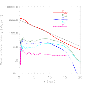
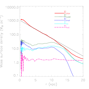
Figure 7: Surface density profiles for the GA2 (left panel) and AqC5 (right panel) simulations, at redshift $z=0$. Red solid line is the stellar profile, gray dotted line the cold gas profile, blue dashed line the molecular hydrogen profile, cyan dotted-dashed line the neutral hydrogen profile, pink triple dotted-dashed line the hot gas profile. The black solid line is the exponential fit to the stellar surface density profile within the (4–12) kpc radial range.

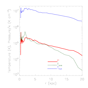
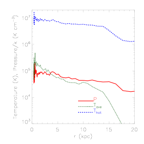
Figure 8: Properties of the ISM in the GA2 (left panel) and AqC5 (right panel) simulations, at redshift $z=0$. In each panel, red continuous line shows the pressure profile; grey dotted line the average cold gas temperature profile; blue dashed line the hot gas temperature profile. The average cold gas temperature is computed using only cold ($T<10^{5}$K) and multi-phase gas particles, and it is weighted using the cold gas mass. Hot gas temperature is mass-weighted.

Figure 9 shows the standard Schmidt-Kennicutt (SK) relation, gas total surface density versus SFR surface density, for our simulated galaxies, again at redshift $z=0$. As discussed in Monaco et al. (2012), we do not impose the SK relation to our star formation prescription, but obtain it as a natural prediction of our model. Contours show observational results from the THINGS galaxies by Bigiel et al. (2008); lines refer to the two simulations. Because gas surface density profile is flat, points tend to cluster at large values of surface densities. Simulations stay well within the observational relation. As also pointed out in Monaco et al. (2012), the simulated relation tends to have a slope of 1.4, which is somewhat steeper than that of $1-1.2$ found for the THINGS galaxies. Furthermore, the external regions of simulated galaxies tend to assume relatively low values of $\Sigma_{\rm sfr}$.

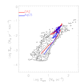
Figure 9: Schmidt-Kennicut relation for the GA2 (red) and AqC5 (blue) simulations. Contours show observational results from THINGS (Bigiel et al. 2008).

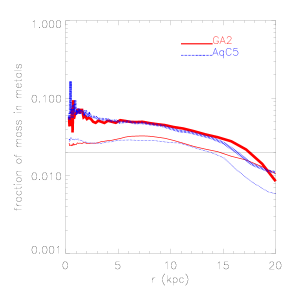
Figure 10: Metallicity profiles for our GA2 (red continuous and dashed lines) and AqC5 (blue dotted and dotted-dashed lines) simulations at $z=0$. Thick and thin lines refer to gas metallicity and stellar total metallicity, respectively. The horizontal thin line is the solar value of the metallicity.

Figure 10 shows the total metallicity profiles for our simulated galaxies, both for the stellar (thin lines) and for the gas (thick lines) component. We used both cold and hot gas for the latter profile. These profiles are very similar for the two galaxies. Stellar metallicity profiles are rather flat in the inner 10 kpc, with values of about $1.5Z_{\odot}$. On the contrary, gas metallicities profiles, that can be more directly compared with observations, get values of $\sim(3-4)Z_{\odot}$ at the center and have gradients of $\sim 0.02$ dex/kpc. These values are relatively flat if compared to the Milky Way ($\sim 0.06$ dex/kpc, e.g. Mott et al., 2013, and references therein) but are similar to those of M31 (Matteucci & Spitoni, 2014, and references therein). The tendency of simulations to produce relatively flat abundance profiles was already noticed by Kobayashi & Nakasato (2011) and Pilkington et al. (2012).

Finally, Figure 11 shows the volume density profile for the stellar, gaseous and DM components. The black line denotes a power law of slope $-1$. In both simulated galaxies, stars dominate over the DM at small radii, $r<3$ kpc. The depletion of gas in the inner 10 kpc, due to both star formation and feedback, produces the sharp decrease of the corresponding density profile. We note that, in the inner 3 kpc, the profile of the DM is shallower than the $-1$ slope predicted by Navarro et al. (1996). This flattening could be due to baryonic processes, e.g the SNe feedback, as suggested also recently e.g. by Governato et al. (2012), Pontzen & Governato (2013) and Zolotov et al. (2012) who carried out simulations at significantly higher resolution. In fact, as a caveat, we remind that our resolution is formally just sufficient to resolve the scales where a flatter DM density profiles is detected.

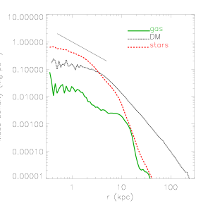
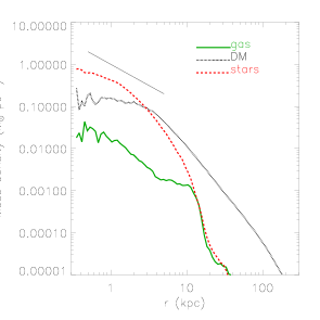
Figure 11: Density profiles of various components for GA2 (left panel) and AqC5 (right panel) simulations, at $z=0$. Green solid lines show the gas profile, grey dotted lines the DM ones, red dashed lines the stellar ones. The black lines marks the slope $\rho\propto r^{-1}$.

5.3 Evolution

As a first diagnostic of the evolution of our simulated galaxies, we show in Figure 12 the corresponding star formation rates. Here we only plot the SFR relative to star particles which lie inside the galaxy radius $R_{\rm gal}$ at redshift $z=0$. Both simulations have higher star formation rates at higher redshift, as expected. They show a roughly bimodal distribution with a first, relatively narrow peak and a further broad component. GA2 has a more peaky SFR and a substained rate of about 15 M_⊙ yr^-1 between redshift 0.85 and 0.25 (corresponding to a cosmic time of 5 and 8 Gyr respectively), then followed by a slow decline. AqC5 shows a similar behaviour of its SFR, but slightly anticipated. The SFRs at redshift $z=0$ is of about 9 (GA2) and 5 (AqC5) M_⊙ yr^-1. These values are slightly larger than that measured for the Milky Way ($[2-5]$ M_⊙ pc^-2; see e.g. Robitaille & Whitney 2010), but these galaxies are slightly more massive than our Galaxy as well. Using the analytic fit of the main sequence of local star-forming galaxies proposed by Schiminovich et al. (2007), the expected SFRs would be 4.7 (GA2) and 3.6 (AqC5) M_⊙ yr^-1, so these galaxies are well within the rather broad main sequence, though both of them are on the high-SFR side.

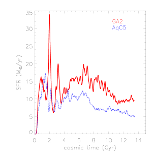
Figure 12: Star formation rates as a function of cosmic time, for simulations AqC5 (blue dotted line) and GA2 (red continuous line). We plot the SFR relative to star particles which lie inside the galaxy radius $R_{\rm gal}$ at redshift $z=0$.

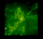
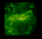
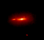
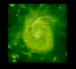
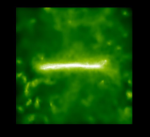
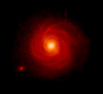
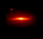
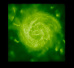
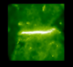
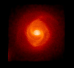
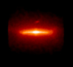
Figure 13: From left to right columns: face-on and edge-on projected gas densities, face-on and edge-on stellar densities for the GA2 simulation, at redshifts $z=2.48$, $2.02$, $1.50$, $1.01$ and $0.49$ (from top to bottom panels). The z-axis of the coordinate system is aligned with the angular momentum vector of the gas enclosed in the inner 8 physical kpc (at all redshifts). Box size is $57$ physical kpc

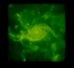
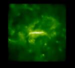
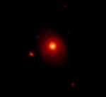
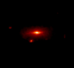
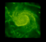
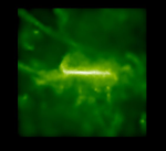
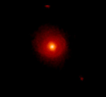
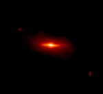
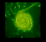
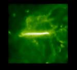
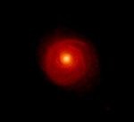
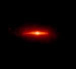
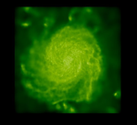
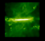
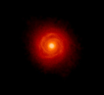
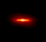
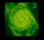
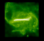
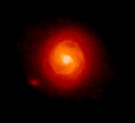
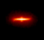
Figure 14: The same as in Figure 13 but for the AqC5 galaxy simulation.

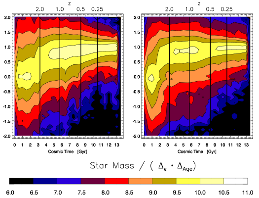
Figure 15: Maps of circularity vs formation time of star particles that at $z=0$ belong to AqC5 (left panel) and GA2 (right panel). Each pixel of the map represents the average star formation in the corresponding interval of circularity. Formation time is binned in intervals of $\Delta t=0.5$ Gyr and circularity in intervals of $0.1$.

Figures 13 and 14 show the density of gas and stars of our simulated galaxies, in face-on and edge-on projections, at redshifts $z=2.48$, $2.02$, $1.50$, $1.01$ and $0.49$. We always align the z-axis of our coordinate systems to the angular momentum vector, evaluated in the inner 8 kpc. In both cases, the inside-out formation of the disk is evident. At the highest redshift, no disk is visible in the GA2 simulation, while an ongoing major merger appears at $z=2.02$. Another minor merger is perturbing the disc at $z=1.50$. Then the accretion history becomes more quiet, with the disk growing in size until the present time. The evolution of AqC5 does not show major merger events, and is overall more quiet. The accretion pattern of the gas of both galaxies is quite complex, with filamentary structures directly feeding the disk. As shown by Murante et al. (2012), gas accreting along these filaments undergoes a significant thermal processing by stellar feedback before it can reach the disc, thereby determining the relative amounts of accreted gas in cold and in warm flows.

Figure 15 shows 2D histograms of circularities and cosmic time of formation of the star particles belonging to the two galaxies at $z=0$. Colours correspond to stellar mass densities in bins of given circularity and age. The corresponding histograms of circularity and radius are shown and commented in Goz et al. (2014). For both simulations, most stars belonging to the bulge and halo components (circularity values around zero) form at high redshift, before $z\approx 2$, corresponding to the first phase of star formation in Figure 12. Stars that belong to the disc component (circularity values around unity) form at lower redshift. These maps illustrate that the formation history of these spiral galaxies can be broadly divided into two events: the formation of bulge and halo components and the formation of the disc, separated by a relatively quiet period. This scenario is in line with the double infall scenario of Chiappini et al. (1997) for the formation of the Milky Way. A similar result was obtained by Cook et al. (2009), who used a cosmological Semi-Analitical Model of galaxy formation and modelled a two-phases formation of disk galaxies. Note that the force resolution of our simulations does not allow us to safely investigate the fine structure of the disk, like separating disk stars into a thin and a thick component. Therefore, a more detailed comparison with the result of galactic archeology models is not feasible at this stage.

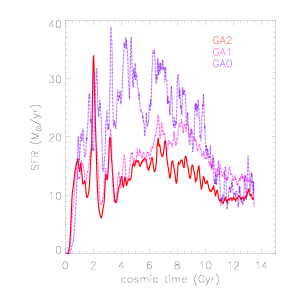
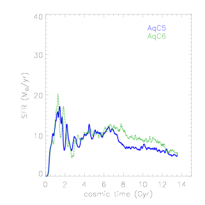
Figure 16: Star formation rate as a function of the cosmic time for GA (left panel) and Aq (right panel) simulations at various resolutions. As for the GA series, purple dashed line refers to GA0, pink dotted line to GA1 and red solid line to GA2. In the right panel we show AqC6 (green dotted line) and AqC5 (blue solid line).

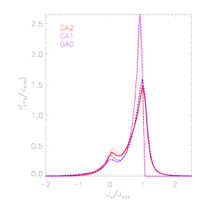
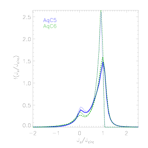
Figure 17: Effect of resolution on the circularity histograms. In the left panel we show the fraction of stellar mass as a function of the circularity for GA0 (purple dotted line), GA1 (pink dashed line) and GA2 (red solid line). In the right panel we show the same for AqC6 (green dotted line) and AqC5 (blue solid line).

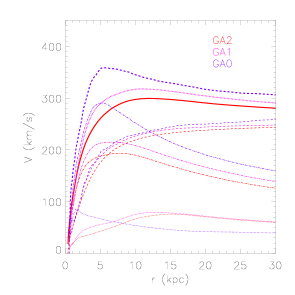
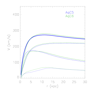
Figure 18: Effect of resolution on the velocity rotation curve. In the left panel we show the velocity rotation curve for simulations GA0 (violet dotted line), GA1 (pink dashed line) and GA2 (red solid line). In the right panel we show the same for AqC6 (green dotted line) and AqC5 (blue solid line).

5.4 Effect of resolution

In this section, we show how our main results change by varying the mass resolution by a factor $\approx 10$ in the Aq series, and by a factor up to $\approx 100$ in the GA series.

The multi-phase model for star formation and feedback that we implemented depends the physical properties of the gas in the simulation. These properties will in general depend on resolution. As a consequence, the resulting feedback efficiency will in turn show a degree of resolution dependence. This was already discussed in M10, based on simulations of idealised spiral galaxies. In cosmological simulations, increasing the resolution does not only imply resolving smaller masses and scales. Initial conditions themselves change as the resolution varies, since more small-scale power is added. Therefore, an exact convergence when resolution is changed is not expected. We also point out that our sub-resolution model has a range of validity, outside which its results are not necessarily reliable. In fact, to properly represent the average density and temperature of gas, we cannot use force resolution that is much larger than the disk height. Because the temperature of the disc is relatively high, a force resolution of several 100 pc is sufficient to properly represent density and pressure. However, when softening increases to $>1$ kpc, density and pressure in a gaseous disk are no longer resolved. As a consequence, we find that the feedback is less efficient. On the other hand, the physical motivation of the model breaks down when the resolution is so accurate to properly resolve single molecular clouds. In this case, a different physical approach is required and additional physical processes must be modelled in order to appropriately describe, at these scales, star formation and SNe feedback.

This said, it is quite remarkable that the results of our model are relatively insensitive to force and mass resolution. In Figure 16 we show the star formation rate as a function of the cosmic time for the GA and Aq simulation series. As in Figure 12, we use only stars within the galactic radius to evaluate the SFR. The GA0 simulation, our lower resolution case, has a remarkably different SFR from GA1 and GA2. On the other hand, GA1 and GA2 produce very similar SFRs for the first seven Gyrs; later, GA1 shows a SFR that is higher by $\approx 40$ per cent at worst, at 9 Gyr, and by less than $30$ per cent at the final epoch. AqC6 and AqC5 show a much better convergence in the SFR, that is almost equal at the end, and differ by less than $\approx 30$ per cent between $t=7$ and $t=12$ Gyr. This is likely to be an effect of the quieter merger history of this halo. We note in general that the SFR is higher when resolution is decreased. In fact, when higher densities and pressures are resolved, feedback is more effective. The effect of enhanced feedback efficiency at higher resolution is to over-compensate the increased amount of available gas, thus resulting in a lower star formation.

In Figure 17 we compare the circularity histograms of our simulated galaxies at $z=0$. The resolution convergence of the GA and Aq galaxies is striking. Only the lowest resolution GA0 shows a very different circularity distribution, with no disk component. Based on this test, we can conclude that already at the resolution of the GA1 simulation, our model is able to produce realistic disk galaxies. From Table 3, it is clear that almost all galaxy properties are very similar between the two resolutions (GA1/AqC6 and GA2/AqC5), with the Aq serie showing better convergence. In particular, the mass of the disk, bulge and gas in these two simulations do not differ by more than $\sim 20$ per cent, while the halo baryon fraction and the fraction of baryons in the galaxy stays within $15$ per cent. The bulge mass of the GA series changes more, but this difference is due to the different action of the stellar bar, which forms at different epochs. In fact, changing the resolution also the timing of mergers and fly-bys may change, thereby changing the epoch of formation of a tidally triggered bar.

In Figure 18 we compare the rotation curves of the two simulation sets, at different resolutions. Also in this case, the Aq series show results that are almost independent of resolution. GA0 shows the largest difference with respect to the other GA curves, with a too strong mass concentration at the centre. GA1 and GA2 show rotation curves that never differ by more than $10$ per cent: at the peak, the difference between the two curves is about $20$ km s^-1, while it decreases to $10$ km s^-1 at 30 kpc.

Given the stability of stellar masses and rotation curves with resolution (except for the case of GA0), also the positions of our simulated galaxies in the Tully-Fisher plot and in the stellar vs. halo mass results to be quite insensitive to numerical resolution.

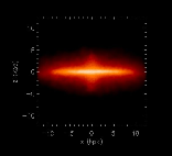
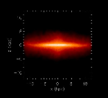
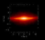
Figure 19: Edge-on view of gas density maps for different values of the Plummer-equivalent gravitational softening: $\epsilon_{Pl}=0.1$, $0.3$, $0.65,1.3$ kpc/h (from left to right panels).

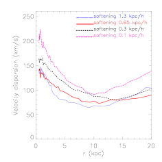
Figure 20: Stellar velocity dispersions along the vertical direction for simulated GA1 galaxies when the softening is changed from $0.1$ to $1.3$ h^-1 kpc, all the other details of the simulation being kept fixed.

Finally, we studied the dependence of our result on the force resolution. To this aim, we repeated the GA1 simulation by changing only the softening scale for the gravitational force. We used $\epsilon_{Pl}=0.1$, $0.3$, $0.65$ (our standard value) and $1.3$ kpc/h (runs sA, sB, sC, SD), for high resolution DM, gas and star particles. In Figure 19 we show edge-on stellar density maps of the corresponding four simulations. Quite remarkably, our reference force resolution sC gives the best defined disk structure. A larger softening produces a well defined disk, but its scale length is significantly smaller. Decreasing the softening has the effect of heating up the disk, due to increased numerical heating. The disk structure is almost lost at our smaller softening value. A more quantitative description of this trend is given in Figure 20, where we show radial profiles of velocity dispersions of stars in the vertical direction. These dispersions are computed as the root means square of the $z$-components of stellar velocities in the galaxy reference frame. In the companion paper by Goz et al. (2014) we show that, due to the existence of broad tails in the velocity distribution, this quantity overestimates the velocity dispersion of disk stars. It is presented here not to quantify the thickness of the disk, but to show how this quantity changes with the softening. There is a clear trend of increasing velocity dispersion with decreasing softening, and this illustrates well how the thickness of the stellar disk is affected by numerical effects, most importantly by 2-body heating. The difference among our reference choice of 0.65 kpc/h and a softening twice as large is relatively small ($\sim$20 per cent), thus indicating that only some residual numerical heating is present at our standard force resolution.

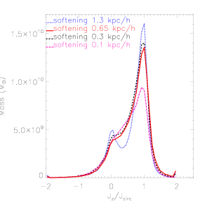
Figure 21: Effect of changing the softening, at fixed mass resolution, on the circularity histograms. We show the stellar mass as a function of the circularity for GA1 simulations when we use a Plummer-equivalent softening length $\epsilon_{Pl}=0.1$ (dotted-dashed magenta line), $0.3$ (dashed black line), $0.65$ (continuous red line), $1.3$ (dotted blue line) kpc/h.

This visual impression is quantitatively confirmed by the analysis of the stellar circularities, shown in Figure 21. The simulation run with our reference value for the softening, and that run with about one half of such a value, have similar circularity histograms with a well defined disk component and a small bulge. The smallest softening produces a drastic change in galaxy properties, with a strong decrease in the disk component. We therefore caution about the use of an aggressive softening in simulations of galaxy formation: numerical heating can damage the disk structure to an amount that exceeds the advantage of a higher force resolution.

6 Conclusions

In this paper we presented results of simulations of disk galaxies, carried out with the GADGET-3 code where we implemented our sub-resolution model for star formation and feedback MUPPI (MUlti Phase Particle Integrator). In our model, differential equations describing the evolution a multi-phase system, that describes the ISM at unresolved scales, are integrated for each multi-phase gas particle. Because cooling times are computed using the density of the local hot phase, thermal energy from SNe is not quickly radiated away. Moreover, no assumption of self-regulation of the multi-phase system is made. As a result, with MUPPI gas particles can hydrodynamically respond to the injection of thermal energy from SNe. With respect to the first version of the code described in Murante et al. (2012), we included the chemical evolution model by Tornatore et al. (2007a), metal cooling as in Wiersma et al. (2009), and a prescription for kinetic feedback.

Our simulations started from zoomed-in cosmological initial conditions of two DM haloes, GA and AqC, at different resolutions. The AqC halo was also simulated by several other groups (e.g. Scannapieco et al., 2009, 2012; Aumer et al., 2013; Marinacci et al., 2013). In our highest resolution run, we use a Plummer-equivalent softening of $\epsilon_{\rm Pl}=0.325$ h^-1 kpc (fixed in physical coordinates since $z=6$), of the same order of magnitude of a typical galaxy disk scale height; our simulation can therefore be described as “moderate resolution” ones.

Our main results can be summarised as follows.

• We obtain disk galaxies with a bulge-over-total stellar mass kinematic ratio $B/T\approx 0.2$, typical of late-type galaxies. The rotation curves are gently rising for 1-2 disk scale radii, and then remain flat. Our simulated galaxies lie within the scatter of the observed Tully-Fisher relation, although on the high side of the allowed range of stellar masses. Our baryon conversion efficiencies are consistently slightly too large, being however within $3\sigma$ from the Moster et al. (2010) relation, and in better agreement with that of Guo et al. (2010) (based on the same cosmology used for AqC5). The fraction of stellar mass in the central galaxy over the total halo mass is of the order of 5 per cent, with a baryon fraction within the virial radius of $0.1$. Stellar density profiles are exponential, with a scale radius of $4.45$ kpc (GA2) and $3.45$ kpc (AqC5). Therefore we consider our simulated galaxies to be “realistic”.

• Our model also provides predictions for several sub-resolution ISM properties: e.g., the amount of molecular gas, and of hot and cold gas. The profiles of such quantities, as well as the total surface density profile of the gas, are rather flat within the inner 10 kpc. Also metallicity profiles are relatively flat. Our disks are gas-rich: the mass of gas is about 30 per cent of the total baryonic disk mass. We obtain a good fit to the observed Schmidt-Kennicutt relation, that is not imposed in the star formation model.

• The evolution of our simulated galaxies is similar to that reported by other authors (e.g. Marinacci et al., 2013; Aumer et al., 2013). The bulge component forms first, while the disk starts to form after $z=2$ and begins to dominate at $z\sim 1$, showing a clear inside-out formation. The star formation rate peaks at a cosmic time of about 2 Gyr, then has a minimum and reaches a new maximum and a mildly decreasing rate. At $z=0$ it reaches values of of 5-10 M_⊙ yr^-1, well within the main sequence of star-forming galaxies. The overall behaviour of bulge formation followed by a minimum of the SFR history and then by the gradual formation of the disc is in line with the two-infall model for the formation of the Milky Way (Chiappini et al., 1997; Cook et al., 2009).

• Our results are rather stable as resolution is decreased by a factor of eight. In particular, morphology-related quantities, such as rotation curves and circularity histograms, vary by less than 10 per cent. Also the SFR varies approximately by the same amount. At lower resolutions, convergence is lost.We note that reducing the softening by a factor six (at fixed mass resolution) induces effects related to numerical heating, thereby severely changing the disk properties. Also, doubling the softening parameter results in a thicker and less extended disk and increases the bulge mass.

It is interesting to compare our results for the AqC5 case with the works by Scannapieco et al. (2009), Scannapieco et al. (2012), Aumer et al. (2013) and Marinacci et al. (2013), who simulated the same halo starting from the same initial conditions. Scannapieco et al. (2009) found that their simulated AqC5 was bulge-dominated: they reported a disk-over-total stellar fraction of 0.21. In the Aquila comparison project (Scannapieco et al., 2012), using the same IC, several group obtained a wide range of galactic properties. An earlier version of MUPPI was included in the comparison and also produced a bulge-dominated galaxy at redshift $z=0$. Aumer et al. (2013) further developed the SF&FB model of Scannapieco et al. (2009) by including kinetic feedback and the effect of radiation pressure by young massive stars. With these implementations, they obtained a disk-dominated galaxy with a flat rotation curve. The circularity diagram that they reported is very similar to that shown here in Fig. 3 However, the baryon conversion efficiency of our simulation is higher than that obtained by Aumer et al. (2013). With the present choice of feedback parameters, the agreement between our results and theirs does not extend to the stellar mass, and, as a consequence, to the position of the AqC5 simulations on the Tully-Fisher relation.

Using AREPO (Springel, 2010), Marinacci et al. (2013) showed a similar result on their simulated AqC5. In their case, the bulge component is slightly more prominent than in our simulations, but also their simulation produced a galaxy which is clearly disk-like and has a dimension similar to what we obtain: their disk scale-length is $R_{d}=3.11$ kpc and the disk mass is $6.07\cdot 10^{10}$ M_⊙, while our AqC5 has $R_{d}=3.42$ kpc and a disk mass of $5.66\cdot 10^{10}$ M_⊙. The agreement between results obtained in this work and those presented in Marinacci et al. (2013) extends to the position on the simulated galaxy in the TF relation and in the stellar vs halo mass one, the shape and normalisation of the rotation curve, and the stability with the resolution. It is worth noticing that the SF&FB models of the three works are quite different, and Marinacci et al. (2013) one also includes black hole feedback.

It is worth pointing out that our results have been obtained at moderate resolution, without resorting to early stellar feedback, to a high threshold for star formation or to a delayed cooling. The ERIS simulation (Guedes et al., 2011) also has realistic properties, in the sense defined above. However, their mass resolution is more than 200 times better than ours for the AqC6 case, that is already “realistic”. Therefore, the possibility of obtaining realistic disk galaxies at moderate resolution and the remarkable numerical convergence of our results open the perspective of simulating large volumes of the universe, containing a representative population of galaxies, with a high, but affordable, computational cost. This is the natural prosecution of the current work and will be the subject of forthcoming papers. At the same time, we must be aware that our simulations still tend to produce stellar disks that are still somewhat too massive. This suggests that we may need to introduce in our simulations other feedback sources which are able to further regulate star formation. In this respect, AGN feedback resulting from gas accretion onto super-massive BHs appears as an obvious missing ingredient.

The agreement of results presented here with those obtained, using the same IC, by other groups, is promising. It is interesting that now, several different models are able to produce realistic disk galaxies, and to obtain, using the same initial condition, very similar results. SF&FBprescriptions share the ability to suppress star formation at high redshift, and favour late-time, high angular momentum gas accretion (see e.g. Übler et al. (2014)). On the other hand, this also means that we are still unable to precisely state which “micro-physical” mechanisms are relevant in galaxy formation and responsible for producing simulated properties in agreement with observations. In fact, the various SF&FB prescriptions used in literarature are not simply different ways to implement the same unresolved processes, but include significantly different combinations and implementations of sub-resolution physics.

However, modern simulations of galaxy formation start being predictive enough that future observations, for instance on the circumgalactic medium, will possibly be able to distinguish among them and, indirectly, tell us what physical processes are needed to form galaxy disks and what other processes are not necessarily involved.

As a final remark, we want to stress again that it is currently not possible to simulate observational properties of galaxies, embedded in a cosmological context, from first physical principles. Therefore, there is no a-priori reason to prefer any sub-resolution prescription upon any other, or a given value for a model parameter, e.g. the density threshold for the onset of star formation. Sub-resolution models can only be judged on the basis of being physically motivated and falsifiable through a detailed comparison with observational data of ever-increasing quality. Codesto solo oggi possiamo dirti, cio’ che non siamo, cio’ che non vogliamo. (Montale, 1923).

References

- Abadi et al. (2003) Abadi, M. G., Navarro, J. F., Steinmetz, M., & Eke, V. R. 2003, ApJ, 597, 21, astro-ph/0212282
- Agertz et al. (2011) Agertz, O., Teyssier, R., & Moore, B. 2011, MNRAS, 410, 1391, 1004.0005
- Aumer et al. (2013) Aumer, M., White, S. D. M., Naab, T., & Scannapieco, C. 2013, MNRAS, 434, 3142, 1304.1559
- Barai et al. (2013) Barai, P. et al. 2013, MNRAS, 430, 3213, 1210.3582
- Barnes & Hernquist (1991) Barnes, J. E., & Hernquist, L. E. 1991, ApJ, 370, L65
- Bigiel et al. (2008) Bigiel, F., Leroy, A., Walter, F., Brinks, E., de Blok, W. J. G., Madore, B., & Thornley, M. D. 2008, AJ, 136, 2846, 0810.2541
- Blitz & Rosolowsky (2006) Blitz, L., & Rosolowsky, E. 2006, ApJ, 650, 933, arXiv:astro-ph/0605035
- Booth & Schaye (2009) Booth, C. M., & Schaye, J. 2009, MNRAS, 398, 53, 0904.2572
- Booth et al. (2007) Booth, C. M., Theuns, T., & Okamoto, T. 2007, MNRAS, 376, 1588, arXiv:astro-ph/0701877
- Brook et al. (2011) Brook, C. B. et al. 2011, MNRAS, 415, 1051, 1010.1004
- Bryan & Norman (2000) Bryan, G. L., & Norman, M. L. 2000, Institute for Mathematics and Its Applications, 117, 165
- Carraro et al. (1998) Carraro, G., Lia, C., & Chiosi, C. 1998, MNRAS, 297, 1021, astro-ph/9712307
- Cen (2014) Cen, R. 2014, ApJ, 781, 38, 1311.5916
- Cen & Ostriker (1993) Cen, R., & Ostriker, J. P. 1993, ApJ, 417, 415
- Ceverino & Klypin (2009) Ceverino, D., & Klypin, A. 2009, ApJ, 695, 292, 0712.3285
- Chabrier (2003) Chabrier, G. 2003, PASP, 115, 763, astro-ph/0304382
- Chiappini et al. (1997) Chiappini, C., Matteucci, F., & Gratton, R. 1997, ApJ, 477, 765, astro-ph/9609199
- Choi & Nagamine (2011) Choi, J.-H., & Nagamine, K. 2011, MNRAS, 410, 2579, 1001.3525
- Christensen et al. (2012) Christensen, C., Quinn, T., Governato, F., Stilp, A., Shen, S., & Wadsley, J. 2012, MNRAS, 425, 3058, 1205.5567
- Christensen et al. (2014) Christensen, C. R., Brooks, A. M., Fisher, D. B., Governato, F., McCleary, J., Quinn, T. R., Shen, S., & Wadsley, J. 2014, MNRAS, 1402.2702
- Colín et al. (2010) Colín, P., Avila-Reese, V., Vázquez-Semadeni, E., Valenzuela, O., & Ceverino, D. 2010, ApJ, 713, 535, 0912.4298
- Cook et al. (2009) Cook, M., Lapi, A., & Granato, G. L. 2009, MNRAS, 397, 534, 0903.2390
- Courteau et al. (2007) Courteau, S., Dutton, A. A., van den Bosch, F. C., MacArthur, L. A., Dekel, A., McIntosh, D. H., & Dale, D. A. 2007, ApJ, 671, 203, 0708.0422
- Crain et al. (2009) Crain, R. A. et al. 2009, MNRAS, 399, 1773, 0906.4350
- Dalla Vecchia & Schaye (2008) Dalla Vecchia, C., & Schaye, J. 2008, MNRAS, 387, 1431, arXiv:0801.2770
- Dalla Vecchia & Schaye (2012) ——. 2012, MNRAS, 426, 140, 1203.5667
- Di Matteo et al. (2003) Di Matteo, T., Croft, R. A. C., Springel, V., & Hernquist, L. 2003, ApJ, 593, 56, astro-ph/0301586
- D’Onghia et al. (2006) D’Onghia, E., Burkert, A., Murante, G., & Khochfar, S. 2006, MNRAS, 372, 1525, arXiv:astro-ph/0602005
- Dutton et al. (2011) Dutton, A. A. et al. 2011, MNRAS, 416, 322, 1012.5859
- Evrard (1988) Evrard, A. E. 1988, MNRAS, 235, 911
- Genel et al. (2014) Genel, S. et al. 2014, ArXiv e-prints, 1405.3749
- Gerritsen & Icke (1997) Gerritsen, J. P. E., & Icke, V. 1997, A&A, 325, 972
- Governato et al. (2010) Governato, F. et al. 2010, Nature, 463, 203, 0911.2237
- Governato et al. (2004) ——. 2004, ApJ, 607, 688, astro-ph/0207044
- Governato et al. (2007) Governato, F., Willman, B., Mayer, L., Brooks, A., Stinson, G., Valenzuela, O., Wadsley, J., & Quinn, T. 2007, MNRAS, 374, 1479, arXiv:astro-ph/0602351
- Governato et al. (2012) Governato, F. et al. 2012, MNRAS, 422, 1231, 1202.0554
- Guedes et al. (2011) Guedes, J., Callegari, S., Madau, P., & Mayer, L. 2011, ApJ, 742, 76, 1103.6030
- Guo et al. (2010) Guo, Q., White, S., Li, C., & Boylan-Kolchin, M. 2010, MNRAS, 404, 1111, 0909.4305
- Haardt & Madau (2001) Haardt, F., & Madau, P. 2001, in Clusters of Galaxies and the High Redshift Universe Observed in X-rays, ed. D. M. Neumann & J. T. V. Tran, astro-ph/0106018
- Hernquist (1989) Hernquist, L. 1989, Nature, 340, 687
- Hernquist & Katz (1989) Hernquist, L., & Katz, N. 1989, ApJS, 70, 419
- Hiotelis & Voglis (1991) Hiotelis, N., & Voglis, N. 1991, A&A, 243, 333
- Hirschmann et al. (2013a) Hirschmann, M., Dolag, K., Saro, A., Borgani, S., & Burkert, A. 2013a, ArXiv e-prints, 1308.0333
- Hirschmann et al. (2013b) Hirschmann, M. et al. 2013b, MNRAS, 436, 2929, 1309.2946
- Hopkins et al. (2013) Hopkins, P. F., Keres, D., Onorbe, J., Faucher-Giguere, C.-A., Quataert, E., Murray, N., & Bullock, J. S. 2013, ArXiv e-prints, 1311.2073
- Hopkins et al. (2011) Hopkins, P. F., Quataert, E., & Murray, N. 2011, MNRAS, 417, 950, 1101.4940
- Ianjamasimanana et al. (2012) Ianjamasimanana, R., de Blok, W. J. G., Walter, F., & Heald, G. H. 2012, AJ, 144, 96, 1207.5041
- Joung et al. (2009) Joung, M. R., Cen, R., & Bryan, G. L. 2009, ApJ, 692, L1, 0805.3150
- Jubelgas et al. (2008) Jubelgas, M., Springel, V., Enßlin, T., & Pfrommer, C. 2008, A&A, 481, 33, astro-ph/0603485
- Katz & Gunn (1991) Katz, N., & Gunn, J. E. 1991, ApJ, 377, 365
- Katz et al. (1992) Katz, N., Hernquist, L., & Weinberg, D. H. 1992, ApJ, 399, L109
- Katz et al. (1996) Katz, N., Weinberg, D. H., & Hernquist, L. 1996, ApJS, 105, 19, arXiv:astro-ph/9509107
- Kennicutt (1998) Kennicutt, Jr., R. C. 1998, ApJ, 498, 541, arXiv:astro-ph/9712213
- Kobayashi & Nakasato (2011) Kobayashi, C., & Nakasato, N. 2011, ApJ, 729, 16, 1012.5144
- Kobayashi et al. (2007) Kobayashi, C., Springel, V., & White, S. D. M. 2007, MNRAS, 376, 1465, astro-ph/0604107
- Kravtsov et al. (1997) Kravtsov, A. V., Klypin, A. A., & Khokhlov, A. M. 1997, ApJS, 111, 73, astro-ph/9701195
- Kroupa et al. (1993) Kroupa, P., Tout, C. A., & Gilmore, G. 1993, MNRAS, 262, 545
- Lia & Carraro (2000) Lia, C., & Carraro, G. 2000, MNRAS, 314, 145, astro-ph/9912098
- Marinacci et al. (2013) Marinacci, F., Pakmor, R., & Springel, V. 2013, MNRAS, 1305.5360
- Marri & White (2003) Marri, S., & White, S. D. M. 2003, MNRAS, 345, 561, astro-ph/0207448
- Martin (2005) Martin, C. L. 2005, ApJ, 621, 227, astro-ph/0410247
- Matteucci & Spitoni (2014) Matteucci, F., & Spitoni, E. 2014, ArXiv e-prints, 1406.0615
- Mayer et al. (2008) Mayer, L., Governato, F., & Kaufmann, T. 2008, Advanced Science Letters, 1, 7, 0801.3845
- Mihos & Hernquist (1996) Mihos, J. C., & Hernquist, L. 1996, ApJ, 464, 641, astro-ph/9512099
- Monaco (2004a) Monaco, P. 2004a, MNRAS, 352, 181, arXiv:astro-ph/0404245
- Monaco (2004b) ——. 2004b, MNRAS, 352, 181, astro-ph/0404245
- Monaco et al. (2012) Monaco, P., Murante, G., Borgani, S., & Dolag, K. 2012, MNRAS, 421, 2485, 1109.0484
- Montale (1923) Montale, E. 1923, in Ossi di seppia, ed. P. Gobetti
- Moster et al. (2010) Moster, B. P., Somerville, R. S., Maulbetsch, C., van den Bosch, F. C., Macciò, A. V., Naab, T., & Oser, L. 2010, ApJ, 710, 903, 0903.4682
- Mott et al. (2013) Mott, A., Spitoni, E., & Matteucci, F. 2013, MNRAS, 435, 2918, 1308.1549
- Murante et al. (2012) Murante, G., Calabrese, M., De Lucia, G., Monaco, P., Borgani, S., & Dolag, K. 2012, ApJ, 749, L34, 1202.5212
- Murante et al. (2010) Murante, G., Monaco, P., Giovalli, M., Borgani, S., & Diaferio, A. 2010, MNRAS, 405, 1491, 1002.4122
- Murray et al. (2005) Murray, N., Quataert, E., & Thompson, T. A. 2005, ApJ, 618, 569, astro-ph/0406070
- Nagamine et al. (2004) Nagamine, K., Springel, V., Hernquist, L., & Machacek, M. 2004, MNRAS, 350, 385, astro-ph/0311295
- Navarro & Benz (1991) Navarro, J. F., & Benz, W. 1991, ApJ, 380, 320
- Navarro et al. (1996) Navarro, J. F., Frenk, C. S., & White, S. D. M. 1996, ApJ, 462, 563, arXiv:astro-ph/9508025
- Navarro & Steinmetz (1997) Navarro, J. F., & Steinmetz, M. 1997, ApJ, 478, 13, astro-ph/9605043
- Navarro & Steinmetz (2000) ——. 2000, ApJ, 538, 477, astro-ph/0001003
- Navarro & White (1994a) Navarro, J. F., & White, S. D. M. 1994a, MNRAS, 267, 401
- Navarro & White (1994b) ——. 1994b, MNRAS, 267, 401
- Night et al. (2006) Night, C., Nagamine, K., Springel, V., & Hernquist, L. 2006, MNRAS, 366, 705, astro-ph/0503631
- Okamoto et al. (2005) Okamoto, T., Eke, V. R., Frenk, C. S., & Jenkins, A. 2005, MNRAS, 363, 1299, astro-ph/0503676
- Okamoto et al. (2010) Okamoto, T., Frenk, C. S., Jenkins, A., & Theuns, T. 2010, MNRAS, 406, 208, 0909.0265
- Oppenheimer & Davé (2006) Oppenheimer, B. D., & Davé, R. 2006, MNRAS, 373, 1265, astro-ph/0605651
- Oser et al. (2010) Oser, L., Ostriker, J. P., Naab, T., Johansson, P. H., & Burkert, A. 2010, ApJ, 725, 2312, 1010.1381
- Padovani & Matteucci (1993) Padovani, P., & Matteucci, F. 1993, ApJ, 416, 26
- Papastergis et al. (2011) Papastergis, E., Martin, A. M., Giovanelli, R., & Haynes, M. P. 2011, ApJ, 739, 38, 1106.0710
- Pilkington et al. (2012) Pilkington, K. et al. 2012, MNRAS, 425, 969, 1205.4796
- Piontek & Steinmetz (2011) Piontek, F., & Steinmetz, M. 2011, MNRAS, 410, 2625, 0909.4156
- Pizagno et al. (2007) Pizagno, J. et al. 2007, AJ, 134, 945, astro-ph/0608472
- Planelles et al. (2013) Planelles, S., Borgani, S., Dolag, K., Ettori, S., Fabjan, D., Murante, G., & Tornatore, L. 2013, MNRAS, 431, 1487, 1209.5058
- Pontzen & Governato (2013) Pontzen, A., & Governato, F. 2013, MNRAS, 430, 121, 1210.1849
- Puchwein & Springel (2013) Puchwein, E., & Springel, V. 2013, MNRAS, 428, 2966, 1205.2694
- Robertson et al. (2004) Robertson, B., Yoshida, N., Springel, V., & Hernquist, L. 2004, ApJ, 606, 32, astro-ph/0401252
- Robitaille & Whitney (2010) Robitaille, T. P., & Whitney, B. A. 2010, ApJ, 710, L11, 1001.3672
- Sales et al. (2010) Sales, L. V., Navarro, J. F., Schaye, J., Dalla Vecchia, C., Springel, V., & Booth, C. M. 2010, MNRAS, 409, 1541, 1004.5386
- Scannapieco et al. (2010) Scannapieco, C., Gadotti, D. A., Jonsson, P., & White, S. D. M. 2010, MNRAS, 407, L41, 1001.4890
- Scannapieco et al. (2012) Scannapieco, C. et al. 2012, MNRAS, 423, 1726, 1112.0315
- Scannapieco et al. (2009) Scannapieco, C., White, S. D. M., Springel, V., & Tissera, P. B. 2009, MNRAS, 396, 696, 0812.0976
- Schaye et al. (2014) Schaye, J. et al. 2014, ArXiv e-prints, 1407.7040