Gravitational leptogenesis, C, CP and strong equivalence

Abstract

The origin of matter-antimatter asymmetry is one of the most important outstanding problems at the interface of particle physics and cosmology. Gravitational leptogenesis (baryogenesis) provides a possible mechanism through explicit couplings of spacetime curvature to appropriate lepton (or baryon) currents. In this paper, the idea that these strong equivalence principle violating interactions could be generated automatically through quantum loop effects in curved spacetime is explored, focusing on the realisation of the discrete symmetries C, CP and CPT which must be broken to induce matter-antimatter asymmetry. The related issue of quantum corrections to the dispersion relation for neutrino propagation in curved spacetime is considered within a fully covariant framework.

1 Introduction

The origin of matter-antimatter asymmetry in the universe remains one of the outstanding problems at the interface of particle physics and cosmology. In recent years, fresh impetus has been given to this issue by the development of models where gravity plays a key role in the symmetry breaking dynamics.

The motivation for looking at gravitational leptogenesis arises from a critical analysis of the Sakharov conditions Sakharov for the generation of matter-antimatter asymmetry in cosmology. These require models of lepto/baryogenesis to contain (i) a mechanism for lepton/baryon number violation,  (ii) C and CP violation,  (iii) non-equilibrium dynamics. Subsequently, it was realised that in a gravitational field, the final criterion may be replaced by an effective violation of CPT symmetry Cohen:1987vi . Models with C and CP-violating gravitational couplings introduced by hand in a more or less well-motivated way have also been proposed to address the second Sakharov condition (see e.g. ref.Lambiase:2013haa for a review). An important example is the interaction $\partial_{\mu}RJ^{\mu}$, where $J^{\mu}$ is the lepton current, introduced in the model of ref.Davoudiasl:2004gf . Here, the time derivative of the Ricci scalar, $\dot{R}$, may act as a chemical potential for lepton number, inducing a lepton-antilepton asymmetry at non-zero temperature.

On the other hand, it is known that in quantum field theory in curved spacetime, quantum loop effects induce effective violations of the strong equivalence principle in the sense that the corresponding effective Lagrangian contains interaction terms which depend explicitly on the curvature, such as $R_{\mu\nu\rho\sigma}F^{\mu\nu}F^{\rho\sigma}$ or $R_{\mu\nu}\bar{\psi}\gamma^{\mu}D^{\nu}\psi$  Drummond:1979pp ; Ohkuwa:1980jx . The question naturally arises whether we can use this mechanism of radiatively-induced strong equivalence violation to automatically generate curvature interactions relevant for leptogenesis. Moreover, a better understanding of the mechanism – especially of the role of the discrete symmetries C, P and T and the key combinations CP and CPT – should provide a guide to the properties of BSM models necessary for gravitational leptogenesis to work. The purpose of this paper is to develop a better theoretical understanding of these fundamental issues.

We should be clear to distinguish two interpretations of “symmetry breaking” in this context. First there is the question of whether the full terms arising in the effective Lagrangian, including the curvature, are invariant under the symmetries of the original theory; in particular, whether discrete symmetries present at tree level may be violated by quantum loop effects. For example, we may ask whether an interaction of the form $\partial_{\mu}R\bar{\psi}\gamma^{\mu}\psi$, which is CP odd, can arise from a CP-conserving tree-level action. We refer to this as “anomalous symmetry breaking”. For this, we require a careful discussion of the realisation of discrete symmetries in a spinor theory in curved spacetime.

However, at a given point in spacetime where the background curvature takes a fixed value, the effective Lagrangian resembles the Lorentz and CPT-violating actions proposed by Kostelecky and collaborators Colladay:1998fq , with the background field curvature playing the role of coupling constants for potentially C, CP or CPT-violating operators. For example, the Lorentz-violating Dirac action contains a term $a_{\mu}\bar{\psi}\gamma^{\mu}\psi$ where the coupling constant $a_{\mu}$ multiplies an operator which is CPT odd. It follows that in a fixed background, the radiatively-induced curvature interactions may effectively violate these discrete symmetries, giving rise to phenomenological effects comparable to those in explicit Lorentz-violating theories. We will refer to this as “environmental symmetry breaking” to emphasise the distinction.

Although we are primarily motivated by possible applications to leptogenesis, the paper is also concerned with more general theoretical issues related to quantum loop effects in spinor field theories in curved spacetime, especially gravitational effects on neutrino propagation. In fact, these are closely related since any gravity-induced change in the neutrino dispersion relation which distinguishes between left and right-handed fermions would induce a matter-antimatter asymmetry.

The paper is organised as follows. In section 2, we present a fully covariant derivation of the dispersion relation for Dirac fermions propagating in curved spacetime, in the framework of the eikonal approximation. Establishing and understanding this requires a careful treatment of the role of local inertial frames and the spin connection, so we begin with an extended discussion of the geometry of spinors in curved spacetime. This discussion sharpens our critique of a number of proposals in the literature, in particular the suggestion in refs.Singh:2003sp ; Mukhopadhyay:2005gb ; Debnath:2005wk that leptogenesis can arise simply through the coupling of neutrinos to the spin connection in the tree-level Dirac action.

Section 3 contains our main analysis of the effective violation of the strong equivalence principle by quantum loops in the case of neutrinos in the standard model. We determine the one-loop effective Lagrangian, emphasising the importance of using a complete basis of hermitian operators, by matching coefficients with explicit Feynman diagram calculations in a weak background field. This generalises earlier work on neutrino propagation in curved spacetime by Ohkuwa Ohkuwa:1980jx .

We then analyse in some detail the discrete symmetry properties of the operators arising in the effective Lagrangian. We verify that in this model, only CP even operators arise, respecting the symmetries of the original tree-level action. There is no evidence, even in curved spacetime, for an anomalous violation of C, CP or CPT symmetry at the quantum loop level. In particular, a CP-violating interaction $\partial_{\mu}R~{}\overline{\nu}_{R}\gamma^{\mu}\nu_{L}$ of the type required by the Davoudiasl et al. model of leptogenesis Davoudiasl:2004gf does not arise through radiative corrections in the CP-conserving sector of the standard model. We conclude that such curvature interactions would only arise in theories in which some CP violation is already present in the original Lagrangian.

Applications of strong equivalence violating curvature interactions in gravitational leptogenesis generally rely either on identifying an interaction as analogous to a chemical potential for lepton number or inferring a splitting in energy levels for particles and antiparticles through dispersion relations. With this motivation, in section 4 we study in some detail the dispersion relations arising from the operators which appear in the effective Lagrangian of section 3, also including the CP-violating operator described above. The occurrence of a hierarchy of scales when curvature interactions are present requires some generalisation of the eikonal approximation discussed in section 2. This also allows us to determine the quantum loop corrections to the neutrino dispersion relation in the standard model, verifying the result of Ohkuwa:1980jx that the low-frequency phase velocity for massless neutrinos is superluminal for backgrounds satisfying the null-energy condition.

Finally, in section 5, we summarise our conclusions and discuss the implication of the theoretical issues raised in our work to models which attempt to generate matter-antimatter asymmetry through gravitational leptogenesis.

2 Inertial Frames and Spinors

2.1 Spinor Formalism in Curved Spacetime

In this section we give a brief review of the main elements of the spinor formalism in curved spacetime we need in the paper (see Bir ; Free for a more complete account). In a general background, Lorentz transformations can only be realised locally in the tangent plane at each spacetime point. This is achieved by introducing an orthonormal basis $\{e_{\mu}^{(a)}\}$ satisfying

$$\eta_{ab}=e_{(a)}^{\mu}e_{(b)}^{\nu}g_{\mu\nu}.$$ (1)

Here, Greek indices label coordinate basis components and Latin indices label the different vierbein basis vectors $a=0,1,2,3$. Lorentz transformations are defined as any transformation of the vierbein

$$e^{\mu}_{(a)}(x)\rightarrow e^{\prime\mu}_{(a)}(x)=\tensor{\Lambda(x)}{{}_{a}^{b}}e^{\mu}_{(b)}(x),$$ (2)

with

$$\Lambda(x)=\exp\left(-\frac{1}{2}\Omega_{ab}(x)M^{ab}\right)$$ (3)

which preserves the relation (1), where $M^{ab}$ form a basis for the fundamental representation of the Lorentz algebra. Thus the vierbein provides a rectangular frame on which one can perform local boosts and rotations.

Now that we have formulated Lorentz transformations, we can introduce particles in the spin-1/2 representation of the Lorentz group. Since the Lorentz transformations are local, this necessitates the introduction of a gauge connection or spin-connection $\omega_{\mu}$ in the spinor representation of the Lorentz algebra

$$\omega_{\mu}=\omega_{\mu}^{ab}\sigma_{ab},$$ (4)

where $\sigma^{ab}=\frac{i}{2}[\gamma^{a},\gamma^{b}]$. The covariant derivative is then defined by

$$D_{\mu}\psi=\left(\partial_{\mu}-\frac{i}{4}\omega_{\mu}^{ab}\sigma_{ab}\right)\psi,$$ (5)

which transforms in the same way as $\psi$ under SO(1,3) transformations:

$$\psi(x)\rightarrow\exp\left(-\frac{i}{2}\Omega_{ab}(x)\sigma^{ab}\right)\psi(x)\equiv D[\Lambda(x)]\psi(x),$$ (6)

provided that the spin connection transforms as

$$\omega^{\mu}_{ab}\rightarrow\tensor{\Lambda}{{}_{a}^{c}}\tensor{\Lambda}{{}_{b}^{d}}\omega^{\mu}_{cd}+\tensor{\Lambda}{{}_{a}^{c}}\partial_{\mu}\Lambda_{bc}$$ (7)

Defining $\gamma^{\mu}=e^{\mu}_{(a)}\gamma^{a}$, one can construct a Lorentz invariant Dirac action

$$\mathcal{L}=\bar{\psi}\left(i\gamma^{\mu}D_{\mu}-m\right)\psi.$$ (8)

One can find a relation between the spin-connection $\omega^{ab}_{\mu}$, vierbein and Christoffel symbols in the following way. Consider a vector $X$. We have that

$$\nabla X =\left(\nabla_{\mu}X^{\nu}\right)dx^{\mu}\otimes\partial_{\nu}$$ (9)

$$=\left(\partial_{\mu}X^{\nu}+\Gamma^{\nu}_{\lambda\mu}X^{\lambda}\right)dx^{\mu}\otimes\partial_{\nu}.$$ (10)

We can also write the derivative in the vierbein basis $\nabla X=\left(\nabla_{\mu}X^{a}\right)dx^{\mu}\otimes e_{(a)}$, which after a little algebra leads to the relation

$$\nabla X=\left(\partial_{\mu}X^{\nu}+e^{\nu}_{(a)}\partial_{\mu}e^{(a)}_{\lambda}X^{\lambda}+e^{\nu}_{(a)}e^{(b)}_{\lambda}\tensor{(\omega_{\mu})}{{}^{a}_{b}}X^{\lambda}\right)dx^{\mu}\otimes\partial_{\nu}.$$ (11)

In order for the expressions (10) and (11) to agree, we must have

$$\tensor{\left(\omega_{\mu}\right)}{{}^{a}_{b}}=e^{(a)}_{\nu}\left(\partial_{\mu}e_{(b)}^{\nu}+\Gamma^{\nu}_{\sigma\mu}e^{\sigma}_{(b)}\right).$$ (12)

With regard to notation, we will use $D_{\mu}$ to denote the derivative which is both a $GL_{4}(\mathbb{R})$ and $SO(1,3)$ tensor. Its action on the vierbein is defined by

$$D_{\mu}e_{\nu}^{(a)}=\partial_{\mu}e^{(a)}_{\nu}-\Gamma_{\nu\mu}^{\sigma}e_{\sigma}^{(a)}-\tensor{(\omega_{\mu})}{{}^{a}_{b}}e^{(b)}_{\nu},$$ (13)

so that (12) is equivalent to the condition

$$D_{\mu}e_{\nu}^{(a)}=0.$$ (14)

We will use $\nabla_{\mu}e_{\nu}^{a}$ to denote the derivative which is a $GL_{4}(\mathbb{R})$ tensor, but not a $SO(1,3)$ tensor:

$$\nabla_{\mu}e^{\nu}_{(a)}=\partial_{\mu}e^{\nu}_{(a)}+\Gamma^{\nu}_{\sigma\mu}e^{\sigma}_{(a)},$$ (15)

This allows the relation (12) to be written in a more compact form as

$$\tensor{\left(\omega_{\mu}\right)}{{}^{a}_{b}}=e^{(a)}_{\nu}\nabla_{\mu}e_{(b)}^{\nu}.$$ (16)

In the next section we introduce the concept of a non-accelerating vierbein frame, and use this together with the relation (16) to show how the spin connection must vanish at the origin of such a frame and hence that the Dirac equation satisfies the strong equivalence principle.

2.2 Inertial Frames

In flat space, the Cartesian tetrad has constant components along any curve, and thus defines an inertial tetrad throughout spacetime. In curved space, an “inertial” tetrad can only be defined in the neighbourhood of a specific reference point corresponding to the inertial observer. The covariant generalisation of “constant components” along a curve is parallel transport.

We construct an inertial frame about a given point $p$ as follows. Choose any orthonormal tetrad $\{e_{(a)}^{\mu}(p)\}$ at $p$ and define the vierbein in the neighbourhood of $p$ by parallel transport of the vierbein along every curve emanating from $p$ (see figure 1). It is now easy to see that the spin connection must vanish at $p$. Pick any coordinate chart $x^{\mu}$ in the neighbourhood of the point $p$, and let $V^{\mu}$ be the tangent vector of any curve through $p$. Then we have

$$V^{\mu}\omega_{\mu}^{cd}=e^{(c)}_{\nu}V^{\mu}\nabla_{\mu}e^{(d)\nu},$$ (17)

but the parallel transport condition means that $V^{\mu}\nabla_{\mu}e^{(d)}=0$ at $p$ and since $V_{\mu}$ is arbitrary it follows that $\omega_{\mu}$ vanishes at $p$. The existence of a local inertial frame is guaranteed by the assumption that the spacetime is Riemannian, the mathematical realisation of the weak equivalence principle.

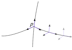
Figure 1: The vierbein is defined in the neighbourhood of $p$ by parallel transport along all curves emanating from $p$.

The physical interpretation is that parallel transport ensures the vierbein, which may be thought of as a set of measuring rods, is not accelerating as it approaches $p$. For a given direction specified by a curve through $p$ with tangent vector $V^{\mu}$ , one can define an acceleration 4-vector $a^{\mu}_{(a)}$ for each vierbein component

$$V\cdot\nabla e^{(a)}_{\mu}=a_{\mu}^{(a)}.$$ (18)

It is then easy to see that our prescription simply imposes the condition that the 4-acceleration of any measuring rod is zero in all directions approaching $p$. Put another way, it means that only observers whose “measuring rods” are accelerating will measure the spin connection at $p$.

Another way to understand the parallel transport condition is to set up Riemann normal coordinates centered on $p$. In these coordinates $\Gamma_{\mu}^{\sigma\rho}(p)=0$ and so the condition $\nabla e^{(a)}(p)=0$ is simply

$$\partial_{\mu}e^{(a)}(p)=0.$$ (19)

In other words, observers with inertial coordinates perceive the inertial vierbein to have constant components in an infinitesimal neighbourhood of $p$. It is now easy to see that for an inertial tetrad the Dirac equation satisfies

$$\mathcal{L}=\bar{\psi}\left(i\not{D}-m\right)\psi\rightarrow\bar{\psi}\left(i\not{\partial}-m\right)\psi,$$ (20)

at $p$. This satisfies the strong equivalence principle, viz. it reduces to its special relativistic form in an inertial frame. As we have seen, this corresponds to the requirement that the curved space Lagrangian involves only the connection, with no explicit curvature terms. We will see how this is affected by quantum corrections later in the paper.

We should also mention that one can define an inertial vierbein along a curve $\gamma$ associated to a geodesic observer with tangent vector $u^{\mu}$ by choosing $e^{(0)}=u$ (with the normalisation $u^{2}=1$) and defining $e^{(i)}$ in the neighborhood by parallel transport along spacelike geodesics normal to $\gamma$. This fixes the SO(1,3) gauge in the normal convex neighbourhood of $\gamma$. One can then define an inertial set of coordinates $x^{\hat{\mu}}$ around $\gamma$ in which the Christoffel symbols vanish along $\gamma$, i.e. $\Gamma_{\hat{\mu}\hat{\nu}}^{\hat{\rho}}(\gamma)=0$. Physically this corresponds to a freely falling observer carrying a gyroscopic set of measuring rods. The full mathematical formulation of this concept is Fermi normal coordinates as discussed at length in Poisson:2011nh .

2.3 Particle Propagation and the Dirac Equation

In curved spacetime, familiar Minkowski space concepts such as particle momenta and trajectories, spin states and dispersion relations are no longer directly applicable and their generalisation requires a subtle and careful analysis of the Dirac equation and its relation to the underlying geometry. Our starting point is the Dirac equation in curved spacetime

$$\left(i\not{D}-m\right)\psi=0.$$ (21)

In flat space, particles are identified with plane waves, but the curved space Dirac equation will not in general admit such solutions. However, in a kinematical regime where the curvature scale is relatively long compared to the wavelength, we can find solutions which locally resemble plane waves and thus exhibit particle-like properties.

To construct these quasi-plane wave solutions, we use an eikonal approach familiar from geometric optics in curved space MTW ; Schneider . These solutions are characterised by a wavelength $\lambda=1/|\underline{k}|\ll L$ where $k_{\mu}$ is the wave-vector and $L$ is the scale over which the amplitude varies (see figure 2).

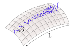
Figure 2: An illustration of the eikonal approximation. The wavelength $\lambda$ is much less than typical curvature scales $L$, so that solutions locally resemble plane waves.

Two other scales enter the analysis – the Compton wavelength of the Dirac particle $\lambda_{c}=1/m$ and the curvature scale $1/\sqrt{\cal{R}}$, where ${\cal{R}}$ represents the size of a typical curvature tensor component. We need to decide from the outset how these relate to the hierarchy of scales $\lambda,L$. Since in the flat-space limit we want to recover the standard dispersion relation $k^{2}-m^{2}=0$, we should clearly take $\lambda_{c}\ll L$. We also identify $1/\sqrt{\cal{R}}$ with $L$, since it is the background gravitational field that determines the scale over which the amplitude of the quasi-plane waves will vary. If we were to take the curvature scale $1/\sqrt{\cal{R}}$ comparable to $\lambda_{c}$ or $\lambda$, the solutions would no longer resemble plane waves and we would lose any interpretation in terms of particle states carrying definite momenta.

In the eikonal approximation, we split the solutions into a rapidly-varying phase $\Theta(x)$ and a slowly-varying amplitude ${\cal A}^{(s)}$ ($s$ = 1,2) multiplying basis spinors $u^{(s)}$ (or $v^{(s)}$ for the corresponding antiparticle solutions), i.e.

$$\psi(x)={\cal A}^{(s)}(x)u^{(s)}(x)e^{-i\Theta(x)/\epsilon},$$ (22)

where

$${\cal A}^{(s)}(x)=a^{(s)}(x)-ib^{(s)}(x)\epsilon-c^{(s)}(x)\epsilon^{2}+\ldots$$ (23)

The book-keeping parameter $\epsilon$ (MTW ; Schneider ), which is finally set to 1, identifies the order of the associated quantities in powers of the parameter $\lambda/L$. We then solve the equation order by order in an expansion in powers of $\epsilon$. To implement the condition $\lambda_{c}\ll L$ automatically, we should also take the mass $m\rightarrow m/\epsilon$ in the Dirac equation (21).

The simplest way to derive the key results, and to compare with previous analyses of the Maxwell equation and photon propagation Shore:2003jx , is to square the Dirac equation and consider the wave equation

$$\left(D^{2}+\frac{m^{2}}{\epsilon^{2}}-\frac{1}{4}R\right)\psi=0$$ (24)

Notice that the Ricci scalar arises from the identity

$$\left[D_{\mu},D_{\nu}\right]\psi=\frac{1}{4}R_{\mu\nu\rho\sigma}\gamma^{\rho}\gamma^{\sigma}\psi$$ (25)

and gamma matrix manipulations. Now insert the eikonal ansatz (22),(23) into (24) and identify $k_{\mu}=\partial_{\mu}\Theta$ as the wave-vector, which is orthogonal to the wavefronts of constant phase $\Theta$. Collecting terms of the same order in $\epsilon$, we find a solution by satisfying the following equations sequentially for $k^{2}$, $a^{(s)}$ and $b^{(s)}$:

$$O(1/\epsilon^{2}): \left(k^{2}-m^{2}\right)a\cdot u=0$$ (26)

$$O(1/\epsilon): -\left[2k\cdot D+\left(D\cdot k\right)\right]a\cdot u+\left(k^{2}-m^{2}\right)b\cdot u=0$$ (27)

$$O(1): \left(D^{2}-\frac{1}{4}R\right)a\cdot u-\left[2k\cdot D+\left(D\cdot k\right)\right]b\cdot u+\left(k^{2}-m^{2}\right)c\cdot u=0,$$ (28)

where $a\cdot u$ is a shorthand for $a^{(s)}u^{(s)}$ with no sum on $s$. Equation (26) recovers the expected dispersion relation

$$k^{2}-m^{2}=0.$$ (29)

To understand the geometric significance of the second equation, consider the congruence defined by the tangent vectors $\hat{k}^{\mu}=g^{\mu\nu}k_{\nu}/m$. These curves, which are timelike geodesics, are identified as the particle trajectories in curved space. The geodesic property follows immediately from (29) by taking a covariant derivative, and using the identity $\nabla_{[\mu}k_{\nu]}=0$, giving the geodesic equation

$$k^{\mu}\nabla_{\mu}k^{\nu}=0.$$ (30)

Defining $\Omega_{\mu\nu}=\nabla_{\mu}\hat{k}_{\nu}$, we may identify the optical scalars $\theta$ (expansion), $\sigma$ (shear) and $\omega$ (twist) of the congruence as

$$\Omega_{\mu\nu}=\frac{1}{3}\theta P_{\mu\nu}+{\sigma}_{\mu\nu}+{\omega}_{\mu\nu},$$ (31)

where we define the projection operator for the hypersurfaces of constant phase by

$$P_{\mu\nu}=g_{\mu\nu}-\hat{k}_{\mu}\hat{k}_{\nu},$$ (32)

and where

$$\theta =\tensor{\Omega}{{}^{\mu}_{\mu}},$$ (33)

$${\sigma}_{\mu\nu} =\Omega_{(\mu\nu)}-\frac{1}{3}\theta P_{\mu\nu},$$ (34)

$$\omega_{\mu\nu} =\Omega_{[\mu\nu]}.$$ (35)

The congruence is twist-free (and therefore surface-forming) by virtue of the fact that $k_{\mu}$ is a gradient, so $\nabla_{[\mu}k_{\nu]}=0$. The divergence measures the rate of expansion of the congruence, $\omega$ measures the tendency of the congruence to twist and the shear $\sigma$ corresponds to geodesics moving apart in one direction and together in the orthogonal direction, whilst preserving the cross-sectional area.

Given $k^{2}=m^{2}$, it follows that the $O(1/\epsilon)$ equation (27) becomes

$$\left[2k\cdot D+\left(D\cdot k\right)\right]a^{(s)}u^{(s)}=0.$$ (36)

If we choose a solution in which the basis spinors $u^{(s)}$ are paralelly transported:

$$k\cdot Du^{(s)}=0,$$ (37)

the equation (36) becomes

$$\hat{k}\cdot Da^{(s)}=-\frac{1}{2}\theta a^{(s)},$$ (38)

which shows that at leading order the amplitude is governed geometrically by the expansion rate of the geodesic congruence. The $O(1)$ equation (28) then determines the sub-leading amplitude correction $b^{(s)}$ in terms of $a^{(s)}$, and so on.

So far, our results are independent of a particular choice of frame. Now, choose a particular timelike geodesic $\gamma$ within the congruence and imagine a co-moving observer freely-falling with the particle along this trajectory, measuring the evolution of its spin polarization. The observer is equipped with an inertial vierbein, where we identify the timelike vierbein component $e^{\mu}_{(0)}$ with $\hat{k}^{\mu}$ and demand that the spatial vierbein vectors $e^{\mu}_{(i)}$ are parallel transported in the neighbourhood of $\gamma$. In this inertial frame the connection vanishes along the trajectory,

$$\omega^{\mu}_{ab}|_{\gamma}=0$$ (39)

Equations (37), (38) then simplify and we have

$$k^{\mu}\partial_{\mu}u^{(s)}|_{\gamma}=0$$ (40)

showing that in this inertial frame the basis spinors are constant along the trajectory, while the amplitude satisfies

$$k^{\mu}\partial_{\mu}a^{(s)}|_{\gamma}=-\frac{1}{2}\theta a^{(s)}$$ (41)

Several key points need to be emphasised here:

1. in the eikonal approximation, we recover a particle interpretation even in curved space, with Dirac particles propagating along timelike geodesics;

2. the connection does not appear in the dispersion relation which, within the eikonal approximation, is identical to its flat space form consistent with the weak and strong equivalence principles;

3. the spin polarisation is parallel propagated along the trajectory, and is constant viewed in an inertial frame;

4. the wave amplitude (particle density) is governed by the expansion optical scalar $\theta$ of the associated geodesic congruence;

5. the curvature only affects the amplitude, not the dispersion relation, and only at higher order in the eikonal approximation as given by (28).

While this reveals the essential physics, and allows an easy comparison with photon propagation, a more rigorous treatment demands that we solve the Dirac equation itself in this framework rather than just the associated wave equation (24). This was first carried out by Audretsch Audretsch:1981wf and we present a simplified version of his analysis here.

Acting with the Dirac operator on the eikonal ansatz (42) and collecting terms of the same order in $\epsilon$ as before, this time we find

$$O(1/\epsilon): \qquad\left(\not{k}-m\right)a\cdot u=0$$ (42)

$$O(1): \qquad\not{D}a\cdot u-\left(\not{k}-m\right)b\cdot u=0$$ (43)

$$O(\epsilon): \qquad\not{D}b\cdot u-\left(\not{k}-m\right)c\cdot u=0$$ (44)

The first equation is now an algebraic matrix equation and the existence of a non-trivial solution requires

$$\det\left(\not{k}-m\right)=0$$ (45)

from which we recover the original dispersion relation $k^{2}-m^{2}=0$. Taking the hermitian conjugate of (42), we see from left multiplying (43) by $\bar{u}^{(s)}$ that

$$\bar{u}^{(s)}\not{D}\left(a^{(s)}u^{(s)}\right)=0$$ (46)

As before we want to choose basis spinors $u^{(s)}$ which satisfy the normalisation

$$\bar{u}^{(r)}\gamma^{\mu}u^{(s)}=\hat{k}^{\mu}\delta^{rs}$$ (47)

and the parallel propagation property

$$\hat{k}^{\mu}D_{\mu}u^{(s)}=0.$$ (48)

One possible choice is

$$u^{(1)}=\left(\frac{E+m}{2m}\right)^{1/2}\left(\begin{array}[]{c}1\\ \\ 0\\ \\ \frac{k^{(3)}}{E+m}\\ \\ \frac{k^{(1)}+ik^{(2)}}{E+m}\end{array}\right),\qquad u^{(2)}=\left(\frac{E+m}{2m}\right)^{1/2}\left(\begin{array}[]{c}0\\ \\ 1\\ \\ \frac{k^{(1)}-ik^{(2)}}{E+m}\\ \\ -\frac{k^{(3)}}{E+m}\end{array}\right),$$ (49)

with

$$E=k^{\mu}e^{(0)}_{\mu},\qquad k^{(i)}=k^{\mu}e^{(i)}_{\mu}.$$ (50)

Taking a covariant derivative of (47) gives

$$\bar{u}^{(r)}\not{D}u^{(s)}=\frac{1}{2}\theta\delta^{rs},$$ (51)

so that expanding (46) as

$$\bar{u}^{(r)}\gamma^{\mu}u^{(s)}D_{\mu}a^{(s)}+a^{(s)}\bar{u}^{(r)}\not{D}u^{(s)}=0$$ (52)

and substituting (47) and (51) gives the evolution of the amplitude as before:

$$k^{\mu}D_{\mu}a^{(s)}=-\frac{1}{2}\theta a^{(s)}.$$ (53)

Finally, we should perhaps emphasise that while this shows that the dispersion relation is independent of the spin connection in the free Dirac Lagrangian, it does not mean that the gravitational field has no influence the dynamics of the fermion’s spin. Indeed, Audretsch Audretsch:1981wf has analysed the propagation of the fermion current $\bar{\psi}\gamma^{\mu}\psi$ in more detail, using a Gordon decomposition into a ‘convection current’ $-i\bar{\psi}\overleftrightarrow{D^{\mu}}\psi$ and a ‘spin magnetisation current’ $(\bar{\psi}\sigma^{\mu\nu}\psi)_{;\nu}$. At leading order in the eikonal expansion, the convection current follows the timelike geodesic defined by $\hat{k}^{\mu}$ (at higher order there are tidal curvature corrections), while the spin motion is defined by parallel propagation.

2.4 Dispersion Relations and Covariance

This analysis allows us to understand better a number of proposals in the literature aimed at exploiting a background gravitational field to induce baryo/leptogenesis through modified dispersion relations.

In a series of papers, Mukhopadhay and others Singh:2003sp ; Mukhopadhyay:2005gb ; Debnath:2005wk have looked for consequences of rewriting the Dirac Lagrangian in the suggestive form

$$\mathcal{L} =\bar{\psi}\left(i\not{D}-m\right)\psi$$ (54)

$$=\bar{\psi}\left(i\gamma^{a}\partial_{a}-m\right)\psi+B_{a}\bar{\psi}\gamma^{a}\gamma^{5}\psi$$ (55)

in a vierbein frame, where

$$B^{d}=\epsilon^{abcd}\left(\omega_{bc}\right)_{a},$$ (56)

and where $\left(\omega_{bc}\right)_{a}=e_{(a)}^{\mu}\left(\omega_{bc}\right)_{\mu}$ is the projection of the spin connection onto the vierbein basis. Since $\bar{\psi}\gamma^{a}\gamma^{5}\psi$ is the spin current, it appears that in a frame where $B_{a}$ is constant, this term acts as a chemical potential which in a theory of neutrinos would induce a particle-antiparticle asymmetry. To establish this, it is claimed Singh:2003sp ; Mukhopadhyay:2005gb ; Debnath:2005wk ; Lambiase:2006md ; Lambiase:2011by ; Lambiase:2013haa that the dispersion relation can be obtained from (55) by considering plane wave solutions of the form $\exp(ip\cdot x)$ giving rise to

$$(p^{a}\pm B^{a})^{2}=m^{2}$$ (57)

for the left and right-handed particles respectively.

However, as we have seen, the true dispersion relations are established in covariant form $p^{2}=m^{2}$. In contrast, equation (57) is not covariant, since $B_{a}$ does not transform as a tensor under the SO(1,3) Lorentz transformations $e_{(a)}\rightarrow\tensor{\Lambda}{{}_{a}^{b}}e_{(b)}$, but rather as

$$B^{a}\rightarrow\tensor{\Lambda}{{}^{a}_{b}}B^{b}+\tensor{\Lambda}{{}^{a}_{b}}\tensor{\Lambda}{{}^{c}_{d}}\varepsilon^{bgdf}\partial_{f}\Lambda_{cg}$$ (58)

Another way to see $B^{a}$ is not an SO(1,3) tensor is to note that we can always make it vanish at a point by $p$ by choosing an inertial vierbein there. Since tensors are either always zero at a point or never zero there, it cannot be a Lorentz tensor.

We conclude, therefore, that equation (57) is not a valid dispersion relation and has no consequence for gravitational leptogenesis. More generally, any leptogenesis model which requires the non-vanishing of the spin connection (e.g. treating $B_{a}$ as a chemical potential), depends on working in a non-inertial, accelerating vierbein where $B_{a}\neq 0$. But this is giving information purely on the nature of the acceleration, not revealing the intrinsic covariant physics. While in some situations it is appropriate to consider non-inertial observers, for cosmological applications the appropriate frame in which to measure lepton density is that of an inertial comoving observer. Thus the free Dirac Lagrangian in curved spacetime does not give rise to gravitational leptogenesis.

We should point out, however, that our conclusions apply to Riemannian spacetimes, where the weak equivalence principle holds and the connection vanishes in local inertial frames. Non-Riemannian geometry, spacetimes with torsion, or string backgrounds with additional antisymmetric and dilaton background fields in addition to the metric Ellis:2013gca may still present interesting generalisations of the picture presented in the last section.

3 Radiatively Induced SEP violation

We now turn to the main topic of this paper, radiatively induced strong equivalence breaking and the realisation of discrete symmetries. Once again, our main focus is on potential applications to gravitational leptogenesis. We are therefore especially interested in the automatic generation by quantum loop effects of operators such as $\partial_{\mu}R\bar{\psi}\gamma^{\mu}\psi$ introduced by hand in the model of Davoudiasl et al. Davoudiasl:2004gf as a C and CP-violating source of matter-antimatter symmetry.

The essential physics behind this effective violation of the strong equivalence principle is readily understood. At the quantum loop level, a particle no longer propagates as a point-like object but is screened by the virtual cloud of particles appearing in its self-energy Feynman diagram Drummond:1979pp ; Ohkuwa:1980jx ; Hollowood:2010bd ; Hollowood:2011yh . As a result, it acquires an effective size characterised by the Compton wavelength of the virtual particles, causing it to experience gravitational tidal forces through its coupling to the background curvature. Particle propagation at the quantum loop level is therefore described by a mean field $\psi$ whose dynamics are described by the effective action $\Gamma$, which gives rise to the quantum-corrected equations of motion

$$\frac{\delta\Gamma}{\delta\bar{\psi}}=0.$$ (59)

As discussed above, many models of gravitational leptogenesis consider interactions of neutrinos with background curvature Davoudiasl:2004gf ; Lambiase:2006md ; Lambiase:2011by ; Lambiase:2013haa . It is therefore interesting to perform a thorough investigation of the effective action for neutrinos propagating in a gravitational background. In this section, we examine the effect of quantum loops on the neutrino dispersion relation, and give a careful discussion of C, P and CP symmetries of the 1-loop effective action.

Since we are interested in the propagation of neutrinos, we consider processes of the form shown in figure 3.

sunset (140,60) i o $\nu$i $\nu$o fermion,tension=2i,v1 fermion,tension=2v2,o photon,label=$Z,,W$,left,tension=0.4v1,v2 fermion,label=$\nu,,e^{-}$v1,v2 the end.Ωend.Ωendinput;

Figure 3: Neutrino Self Energies

The relevant parts of the SM lagrangian, with massless neutrinos, are:

$$\mathcal{L}_{EW}=\sqrt{-g}\Big{[} -\frac{1}{4}g^{\mu\rho}g^{\nu\sigma}\left(2W^{-}_{\mu\nu}W^{+}_{\rho\sigma}+Z_{\mu\nu}Z_{\rho\sigma}\right)$$

$$+g^{\mu\nu}\left(M_{W}^{2}W_{\mu}^{-}W^{+}_{\nu}+\frac{1}{2}M_{Z}^{2}Z_{\mu}Z_{\nu}\right)$$

$$+\bar{e}\left(i{\gamma}\cdot D-m_{e}\right)e+\bar{\nu}_{R}i\gamma\cdot D\nu_{L}$$

$$\frac{g}{\sqrt{2}}\left(\bar{\nu}_{R}\gamma\cdot W^{+}e_{L}+\mbox{h.c}\right)-\frac{g}{2\cos\theta_{W}}\bar{\nu}_{R}\gamma\cdot Z\nu_{L}\Big{]},$$ (60)

where

$$\cos^{2}\theta_{W}=\frac{g^{2}}{g^{\prime 2}+g^{2}},\qquad m_{W}=\cos\theta_{W}m_{Z}$$ (61)

and $g$ and $g^{\prime}$ are SU(2) and U(1) gauge couplings respectively and $W_{\mu\nu}$, $Z_{\mu\nu}$ are the $W$ and $Z$ field strengths. Since there are no infrared divergences in the relevant Feynman diagrams and the electron mass contributes only at $O(m_{e}/m_{W})$, it has no qualitative effect on our analysis and may be neglected.

3.1 Hermiticity

Since we are interested in the free propagation of neutrinos, we need only consider those parts of the effective action quadratic in the mean neutrino field, so that the equations of motion are linear in $\nu$. We construct the effective action for operators up to third order in derivatives by demanding that it is consistent with general covariance and local Lorentz invariance. This is achieved by constructing all possible neutrino bilinears from the contraction of curvature tensors $R,R_{\mu\nu}$ etc. with gamma matrices and neutrino spinors up to the required number of derivatives. Up to third order in derivatives the following set of operators covers all possible combinations:

$$\partial_{\mu}R\bar{\nu}_{R}\gamma^{\mu}\nu_{L},\quad R\bar{\nu}_{R}\not{D}\nu_{L},\quad R_{\mu\nu}\bar{\nu}_{R}\gamma^{\mu}D^{\nu}\nu_{L},\quad\bar{\nu}_{R}D^{2}\not{D}\nu_{L},\quad\bar{\nu}_{R}\not{D}D^{2}\nu_{L},\quad\bar{\nu}_{R}D_{\mu}\not{D}D^{\mu}\nu_{L},$$ (62)

where

$$\nu_{L}=\frac{1-\gamma_{5}}{2}\nu,\qquad\bar{\nu}_{R}=\bar{\nu}\frac{1+\gamma_{5}}{2}.$$ (63)

One might think that it is possible to construct operators from the Riemann tensor $R_{\mu\nu\rho\sigma}$. However the only possible combinations up to third order in derivatives are of the form

$$R_{\mu\nu\rho\sigma}\bar{\nu}_{R}\gamma^{\mu}\gamma^{\nu}\gamma^{\rho}D^{\sigma}\nu_{L},$$ (64)

and so on, since they must involve only an odd number of gamma matrices, but using the Dirac algebra, and in particular the identities $R_{\mu[\nu\rho\sigma]}=0$ and

$$\gamma^{\mu}\gamma^{\nu}\gamma^{\lambda}=g^{\mu\nu}\gamma^{\lambda}+g^{\nu\lambda}\gamma^{\mu}-g^{\mu\lambda}\gamma^{\nu}-i\varepsilon^{\sigma\mu\nu\lambda}\gamma_{\sigma}\gamma_{5},$$ (65)

it is straighforward to show that these reduce to linear combinations of the operators in (62). Finally using the identity

$$\left[D_{\mu},D_{\nu}\right]\nu_{L}=\frac{1}{4}R_{\mu\nu\rho\sigma}\gamma^{\rho}\gamma^{\sigma}\nu_{L}$$ (66)

it can be shown that the final two terms in (62) give a contribution to the action which is a linear combination of other operators:

$$\int d^{4}x\sqrt{-g}\left(\bar{\nu}_{R}D_{\mu}\not{D}D^{\mu}\nu_{L}\right) =\int d^{4}x\sqrt{-g}\left[\frac{1}{2}R^{\mu\nu}\bar{\nu}_{R}\gamma_{\mu}D_{\nu}\nu_{L}+\frac{1}{4}\partial_{\mu}R\bar{\nu}_{R}\gamma^{\mu}\nu_{L}+\bar{\nu}_{R}D^{2}\not{D}\nu_{L}\right]$$ (67)

$$\int d^{4}x\sqrt{-g}\left(\bar{\nu}_{R}\not{D}D^{2}\nu_{L}\right) =\int d^{4}x\sqrt{-g}\left[\frac{1}{4}\partial_{\mu}R\bar{\nu}_{R}\gamma^{\mu}\nu_{L}+\bar{\nu}_{R}D^{2}\not{D}\nu_{L}\right]$$ (68)

In summary then, the list of linearly independent bilinears reduces to

$$\partial_{\mu}R\bar{\nu}_{R}\gamma^{\mu}\nu_{L},\quad R\bar{\nu}_{R}\not{D}\nu_{L},\quad R_{\mu\nu}\bar{\nu}_{R}\gamma^{\mu}D^{\nu}\nu_{L},\quad\bar{\nu}_{R}iD^{2}\not{D}\nu_{L},$$ (69)

and so the most general form of the effective action is

$$\Gamma=\int d^{4}x\sqrt{-g(x)}\Bigg{[} \bar{\nu}_{R}i\not{D}\nu_{L}+\alpha_{1}\partial_{\mu}R\bar{\nu}_{R}\gamma^{\mu}\nu_{L}+\alpha_{2}iR\bar{\nu}_{R}\not{D}\nu_{L}+\alpha_{3}\bar{\nu}_{R}R_{\mu\nu}\gamma^{\mu}iD^{\nu}\nu_{L}+\alpha_{4}\bar{\nu}_{R}iD^{2}\not{D}\nu_{L}\Bigg{]},$$ (70)

where the $\alpha_{i}$ can in general be complex. In order to respect the hermiticity of the full electroweak theory, we must demand that the effective action is hermitian and impose

$$\Gamma^{\dagger}=\Gamma.$$ (71)

At this point our analysis improves on that of Ohkuwa Ohkuwa:1980jx who did not impose the requirement of hermiticity in constructing the effective action. The first operator in (69) is hermitian but the remaining operators are not. They have the following hermiticity properties:

$$\int d^{4}x\sqrt{-g}\left(R\bar{\nu}_{R}i\not{D}\nu_{L}\right)^{\dagger} =\int d^{4}x\sqrt{-g}\left[R\bar{\nu}_{R}i\not{D}\nu_{L}+i\partial_{\mu}R\bar{\nu}_{R}\gamma^{\mu}\nu_{L}\right],$$ (72)

$$\int d^{4}x\sqrt{-g}\left(R_{\mu\nu}\bar{\nu}_{R}\gamma^{\mu}iD^{\nu}\nu_{L}\right)^{\dagger} =\int d^{4}x\sqrt{-g}\left[R_{\mu\nu}\bar{\nu}_{R}\gamma^{\mu}iD^{\nu}\nu_{L}+\frac{1}{2}i\partial_{\mu}R\bar{\nu}_{R}\gamma^{\mu}\nu_{L}\right],$$ (73)

$$\int d^{4}x\sqrt{-g}\left(\bar{\nu}_{R}iD^{2}\not{D}\nu_{L}\right)^{\dagger} =\int d^{4}x\sqrt{-g}\left[\bar{\nu}_{R}iD^{2}\not{D}\nu_{L}+\frac{1}{4}i\partial_{\mu}R\bar{\nu}_{R}\gamma^{\mu}\nu_{L}\right],$$ (74)

We now use these properties and impose the condition (71) to get relations among the $\alpha_{i}$. We find that all the coefficients are all real, with the exception of $\alpha_{1}$, whose imaginary part must satisfy

$$\mbox{Im}(\alpha_{1})=\frac{1}{2}\alpha_{2}+\frac{1}{4}\alpha_{3}+\frac{1}{8}\alpha_{4}.$$ (75)

Hence with a suitable redefinition of the effective coefficients the most general form of the effective action is

$$\Gamma=\int d^{n}x\sqrt{-g(x)}\Bigg{[}\bar{\nu}_{R}i\not{D}\nu_{L} +ia\bar{\nu}_{R}\left(2R_{\mu\nu}\gamma^{\mu}D^{\nu}+\frac{1}{2}\partial_{\mu}R\gamma^{\mu}\right)\nu_{L}$$

$$+b\partial_{\mu}R\bar{\nu}_{R}\gamma^{\mu}\nu_{L}$$

$$+ic\bar{\nu}_{R}\left(2R\not{D}+\partial_{\mu}R\gamma^{\mu}\right)\nu_{L}$$

$$+id\bar{\nu}_{R}\left(2D^{2}\not{D}+\frac{1}{4}\partial_{\mu}R\gamma^{\mu}\right)\nu_{L}\Bigg{]}.$$ (76)

The operators

$$S_{a}= \int d^{n}x\sqrt{-g(x)}~{}i\bar{\nu}_{R}\left[2R_{\mu\nu}\gamma^{\mu}D^{\nu}+\frac{1}{2}\partial_{\mu}R\gamma^{\mu}\right]\nu_{L}$$ (77)

$$S_{b}= \int d^{n}x\sqrt{-g(x)}~{}\partial_{\mu}R\bar{\nu}_{R}\gamma^{\mu}\nu_{L}$$ (78)

$$S_{c}= \int d^{n}x\sqrt{-g(x)}~{}i\bar{\nu}_{R}\left[2R\not{D}+\partial_{\mu}R\gamma^{\mu}\right]\nu_{L}$$ (79)

$$S_{d}= \int d^{n}x\sqrt{-g(x)}~{}i\bar{\nu}_{R}\left[2D^{2}\not{D}+\frac{1}{4}\partial_{\mu}R\gamma^{\mu}\right]\nu_{L}$$ (80)

which appear in $\Gamma$, therefore form a complete set of linearly independent hermitian operators up to third order in derivatives.

3.2 Discrete Symmetries

Since the discrete spacetime symmetries P and T single out particular directions in spacetime, we assume the existence of a vector basis with a timelike vector $e^{(0)}$ and spacelike vectors $e^{(i)}$ which define spatial and temporal directions at each point $x$ in the manifold. We can then define P and T transformations locally at each point $x$ by:

$$P: \qquad\mathcal{P}e^{(a)}(x)\mathcal{P}^{-1}=(-)^{a}e^{(a)}(x),\qquad\mathcal{P}\nu(x)\mathcal{P}^{-1}=\gamma^{0}\nu(x),$$ (81)

$$T: \qquad\mathcal{T}e^{(a)}(x)\mathcal{T}^{-1}=-(-)^{a}e^{(a)}(x),\qquad\mathcal{T}\nu(x)\mathcal{T}^{-1}=B\nu(x),$$ (82)

$$C: \qquad\mathcal{C}\nu(x)\mathcal{C}^{-1}=C\left(\bar{\nu}\right)^{T}(x),$$ (83)

where the notion $(-)^{a}$ is a shorthand defined by

$$(-)^{0}=1,\qquad(-)^{i}=-1,\qquad i=1,2,3.$$ (84)

The matrices satisfy $B^{\dagger}\gamma^{a*}B=(-1)^{a}\gamma^{a}$ and $B^{\dagger}B=1$, $C\gamma^{\mu}C^{-1}=-\gamma^{\mu}$ and $C^{T}=-C$, and $\mathcal{T}$ complex conjugates any complex numbers. This has the consequence that tensor quantities $T^{a_{1}\ldots a_{m}}$ transform as

$$T^{a_{1}\ldots a_{m}}(x)\mapsto\left(\pm 1\right)^{m}(-)^{a_{1}}\cdots(-)^{a_{m}}T^{a_{1}\ldots a_{m}}(x)$$ (85)

where the plus and minus sign correspond to P and T respectively. In particular, since we want $D_{\mu}\psi$ to transform like $\partial_{\mu}\psi$ under $P$ and $T$, it is easy to check that identifying the vector basis above with the vierbein ensures the connection part

$$\Gamma_{c}~{}\psi=-\frac{i}{4}\omega_{c}^{ab}\sigma_{ab}\psi,$$ (86)

(and hence $D_{\mu}\psi$) transforms like $\partial_{\mu}\psi$ under P and T.

Notice that the arguments of the operators do not transoform as $(t,\vec{x})\rightarrow(t,-\vec{x})$, under P etc. as they do in flat space. The reason is that in flat space, the object $x^{\mu}$ is playing the role of a vector (rather than a coordinate) so that $(t,\vec{x})\rightarrow(t,-\vec{x})$ should be thought of as an action on the tangent plane, rather than on coordinates. With an understanding of this subtlety, the generalisation to curved space is immediate, and one sees that P and T are only well-defined as actions on vectors in the tangent plane. For example, in the case of a scalar field, the object $\partial^{\mu}\phi(x)$ should be thought of as a vector in the tangent plane at $x$, which transforms according to (85).

We summarise the C, P, CP and CPT properties of the effective operators in a table below. A full derivation of these results can be found in appendix B:

	$\int d^{4}x\sqrt{-g}~{}\bar{\nu}_{R}i\not{D}\nu_{L}$	$S_{a,c,d}$	$S_{b}$
P	$L\leftrightarrow R$	$L\leftrightarrow R$	$L\leftrightarrow R$
T	+1	$+1$	$-1$
C	$L\leftrightarrow R$	$L\leftrightarrow R$	$-\left(L\leftrightarrow R\right)$
CP	$+1$	$+1$	$-1$
CPT	$+1$	$+1$	$+1$

We see that with the exception of $L_{b}=\partial_{\mu}R\bar{\nu}_{R}\gamma^{\mu}\nu_{L}$ (which importantly is CP odd) all the operators respect the CP, T and CPT symmetries of the tree-level EW Lagrangian. It is thus of great interest to investigate the possibility that the CP violating operator $L_{b}$ is radiatively generated by quantum loop effects. This is particularly pertinent in light of the suggestion by Davoudiasl et al. Davoudiasl:2004gf that effectively generated C and CP-violating operators such as

$${L}_{int}\sim\partial_{\mu}R\bar{\psi}\gamma^{\mu}\psi,$$ (87)

give a chemical potential of the form $\mu\sim\dot{R}$ resulting in a gravitationally induced lepton or baryon asymmetry.

3.3 Matching

We now calculate the coefficients of the curvature terms in the effective action by matching with explicit weak-field Feynman diagram calculations. Since the effective couplings are independent of the choice of geometry, we are free to perform the matching on the most convenient background, providing it is of sufficient generality to distinguish the various terms in the action. The matching is greatly simplified by choosing a conformally flat metric

$$g_{\mu\nu}=K\eta_{\mu\nu},$$ (88)

and conformally rescaled fields

$$e=K^{-(n-1)/4}\tilde{e},\quad Z_{\mu}=K^{-(n-4)/4}\tilde{Z}_{\mu},$$ (89)

and similarly for the other fields. In terms of the conformally rescaled fields, the Lagrangian becomes

$$\mathcal{L}_{EW}= \mathcal{L}_{Maxwell}+\eta^{\mu\nu}K\left(M_{W}^{2}\tilde{W}_{\mu}^{-}\tilde{W}^{+}_{\nu}+\frac{1}{2}M_{Z}^{2}\tilde{Z}_{\mu}\tilde{Z}_{\nu}\right)$$

$$+\bar{\tilde{e}}i\not{\partial}\tilde{e}+\bar{\tilde{\nu}}_{R}i\gamma\not{\partial}\tilde{\nu}_{L}$$

$$+\frac{g}{\sqrt{2}}K^{-(n-4)/4}\left(\bar{\tilde{\nu}}_{R}\not{\tilde{W}}^{+}\tilde{e}_{L}+\mbox{h.c}\right)-\frac{g}{2\cos\theta_{W}}K^{-(n-4)/4}\bar{\tilde{\nu}}_{R}\not{\tilde{Z}}\tilde{\nu}_{L},$$ (90)

where

$$\mathcal{L}_{Maxwell}=\eta^{\mu\rho}\eta^{\nu\sigma}\Bigg{[} -\frac{1}{4}\tilde{Z}_{\mu\nu}\tilde{Z}_{\rho\sigma}$$

$$+\frac{(n-4)}{8}K^{-1}\left(\partial_{\mu}K\cdot\tilde{Z}_{\nu}-\partial_{\nu}K\cdot\tilde{Z}_{\mu}\right)\tilde{Z}_{\rho\sigma}$$

$$-\frac{(n-4)^{2}}{64}K^{-2}\left(\partial_{\mu}K\cdot\tilde{Z}_{\nu}-\partial_{\nu}K\cdot\tilde{Z}_{\mu}\right)\left(\partial_{\rho}K\cdot\tilde{Z}_{\sigma}-\partial_{\sigma}K\cdot\tilde{Z}_{\rho}\right)$$

$$+(\mbox{similar term for $\tilde{W}^{\pm}$})\Bigg{]},$$ (91)

with $\tilde{Z}_{\mu\nu}=\partial_{\mu}\tilde{Z}_{\nu}-\partial_{\mu}\tilde{Z}_{\nu}$. We match by considering

$$K=1+h,$$ (92)

and demanding that the full and effective theories give the same amplitudes at linear order in the classical graviton $h$. There are 3 diagrams linear in $h$ shown in figure 4

graviton3 (100,70) i o g $p$i $p^{\prime}$o $q$g fermion,tension=2i,v1 fermion,tension=2v1,v2 fermion,tension=2v2,o photon,left,tension=0.4v1,v3 photon,right,tension=0.4v2,v3 dashes,tension=0.4v3,g the end.Ωend.Ωendinput;

(a)

graviton1 (100,70) i o g1,g2,g3,g4 fermion,tension=2i,v1 fermion,tension=2v1,v2 fermion,tension=2v2,o photon,left,tension=0.4v1,v2 dashes,tension=0v2,g3 the end.Ωend.Ωendinput;

(b)

graviton2 (100,70) i o g1,g2,g3,g4 fermion,tension=2i,v1 fermion,tension=2v1,v2 fermion,tension=2v2,o photon,left,tension=0.4v1,v2 dashes,tension=0v1,g2 the end.Ωend.Ωendinput;

(c)

Figure 4: Graviton diagrams. The dashed line denotes momentum space contribution from classical graviton. The internal lines denote either $W$ and $e$ or $Z$ and $\nu$.

We use $p^{\mu}$ and $p^{\prime\mu}$ to denote the incoming and outgoing neutrino momenta, and $q^{\mu}=p^{\mu}-p^{\prime\mu}$ to label the graviton momentum. The first of these gives an amplitude of the form

$$i\mathcal{M}_{1}= \left(i{M^{2}}\right)(-ig_{0})^{2}\int\frac{d^{n}k}{(2\pi)^{n}}\frac{i}{(p-k)^{2}-M^{2}}\frac{i\gamma_{\mu}\not{k}\gamma^{\mu}}{k^{2}}\frac{i}{(p-k-q)^{2}-M^{2}}$$

$$= \frac{ig_{0}^{2}}{(4\pi)^{2}M^{2}}\left(\frac{1}{2}\not{q}M^{2}-\not{p}M^{2}+\frac{1}{6}q^{2}\not{q}+\frac{1}{6}p^{2}\not{q}-\frac{2}{9}p\cdot q\not{q}-\frac{5}{18}q^{2}\not{p}+\frac{1}{3}p\cdot q\not{p}-\frac{1}{3}p^{2}\not{p}\right)$$

$$+\mathcal{O}\left(\frac{p^{5}}{M^{4}}\right)$$ (93)

The second diagram gives

$$i\mathcal{M}_{2}=\left(ie\frac{(n-4)}{4}h\right)(-ie)\int\frac{d^{n}k}{(2\pi)^{n}}\frac{i}{(k-p)^{2}-M^{2}}\frac{i\gamma_{\mu}\not{k}\gamma^{\mu}}{k^{2}}~{}~{}\stackrel{{\scriptstyle n\rightarrow 4}}{{=}}~{}~{}i\frac{g_{0}^{2}}{2(4\pi)^{2}}\not{p},$$ (94)

where the $(n-4)$ conformal factor from the graviton vertex combines with the UV divergence of the self energy diagram to produce a finite result. The third diagram is the same as this, but with $p\rightarrow p-q$:

$$i\mathcal{M}_{3}=i\frac{g^{2}_{0}}{2(4\pi)^{2}}\left(\not{p}-\not{q}\right).$$ (95)

When we sum the three diagrams, the terms linear in momentum cancel so there is no finite field renormalization of the free Dirac operator in the effective Lagrangian.

$$\mathcal{M}_{tot}=\frac{g_{0}^{2}}{3(4\pi)^{2}M^{2}}\left(\frac{1}{2}q^{2}\not{q}+\frac{1}{2}p^{2}\not{q}-\frac{2}{3}p\cdot q\not{q}-\frac{5}{6}q^{2}\not{p}+p\cdot q\not{p}-p^{2}\not{p}\right)$$ (96)

We now insert the appropriate couplings and count this amplitude twice for the different particle species in the loop, one with $g_{0}=g/\sqrt{2}$, $M=m_{W}$ and the other with $g_{0}=g/(2\cos\theta_{W})$, $M=m_{Z}$. Using the result $m_{W}^{2}=\cos^{2}\theta_{W}m_{Z}^{2}$ the full amplitude can be written in terms of the SU(2) coupling $g$ and the $W$-boson mass as

$$\mathcal{M}=\frac{1}{4}\frac{g^{2}}{(4\pi)^{2}m_{W}^{2}}\left[\left(-p^{2}+p\cdot q-\frac{5}{6}q^{2}\right)\not{p}+\left(\frac{1}{2}p^{2}-\frac{2}{3}p\cdot q+\frac{1}{2}q^{2}\right)\not{q}\right].$$ (97)

Poles and The Maxwell Term

One might worry that the vertex proportional to $(n-4)$ in the Maxwell term (91) gives a finite contribution to the amplitude for the first diagram in figure 4 due to poles in the loop integral. However, we now show this contribution vanishes. We prove this for the $Z$-boson, with the $W$ following in exactly the same way. The relevant interaction is

$$\mathcal{L}_{int} =\frac{(n-4)}{8}K^{-1}\left(\partial_{\rho}K\cdot\tilde{Z}_{\lambda}-\partial_{\lambda}K\cdot\tilde{Z}_{\rho}\right)\tilde{Z}^{\rho\lambda}$$ (98)

$$=\frac{(n-4)}{4}\partial_{\rho}h\tilde{Z}_{\lambda}\left[\partial^{\rho}\tilde{Z}^{\lambda}-\partial^{\lambda}\tilde{Z}^{\rho}\right],$$ (99)

The amplitude for $\mathcal{L}_{int}$ is given by

$$i\mathcal{M}_{pole}= \frac{(n-4)}{4}\left(-\frac{ig}{2\cos\theta_{W}}\right)^{2}\times$$ (100)

$$\int\frac{d^{n}k}{(2\pi)^{n}}\Bigg{[}\left[q\cdot(p-k-q)-q\cdot(p-k)\right]D_{\mu\lambda}(p-k)\tensor{D}{{}^{\lambda}_{\sigma}}(p-k-q)$$

$$\qquad-q^{\rho}(p-k-q)^{\lambda}D_{\mu\lambda}(p-k)D_{\rho\sigma}(p-k-q)$$

$$\qquad+q^{\rho}(p-k)^{\lambda}D_{\mu\rho}(p-k)D_{\lambda\sigma}(p-k-q)\Bigg{]}\gamma^{\mu}\frac{i\not{k}}{k^{2}}\gamma^{\sigma},$$ (101)

where $D_{\mu\nu}(p)$ is the $\tilde{Z}$ propagator:

$$D_{\mu\nu}(q)=\frac{i\eta_{\mu\nu}}{q^{2}-m_{Z}^{2}}.$$ (102)

Inserting (102), the amplitude reduces to

$$i\mathcal{M}_{pole}=\frac{(n-4)}{16\cos^{2}\theta_{W}}g^{2}\int\frac{d^{n}q}{(2\pi)} \Bigg{[}q_{\mu}(p-k)_{\sigma}-q^{2}\eta_{\mu\sigma}-q_{\sigma}(p-k-q)_{\mu}\Bigg{]}$$

$$\times\frac{i}{(p-k)^{2}-m_{Z}^{2}}\gamma^{\mu}\frac{i\not{k}}{k^{2}}\gamma^{\sigma}\frac{i}{(p-k-q)^{2}-m_{Z}^{2}}$$ (103)

Only terms in the momentum integral which produce a pole in $(n-4)$ will contribute. These come from the highest powers of loop momenta. Retaining only those terms we get

$$i\mathcal{M}_{pole}= \frac{(n-4)}{16\cos^{2}\theta_{W}}g^{2}\int\frac{d^{n}q}{(2\pi)}\left[k_{\mu}q_{\sigma}-k_{\sigma}q_{\mu}\right]\frac{i}{(p-k)^{2}-m_{Z}^{2}}\gamma^{\mu}\frac{i\not{k}}{k^{2}}\gamma^{\sigma}\frac{i}{(p-k-q)^{2}-m_{Z}^{2}}$$

$$+O(n-4),$$ (104)

but

$$\left[k_{\mu}q_{\sigma}-k_{\sigma}q_{\mu}\right]\gamma^{\mu}\not{k}\gamma^{\sigma}=0,$$ (105)

and so the momentum integral vanishes, verifying our claim that there is no contribution in the $n\rightarrow 4$ limit from the Maxwell term.

One can in fact verify the general form of this amplitude (97) as follows. The amplitude for the above process is given by

$$\mathcal{M}(p,q)=\bra{\nu(p)}S\ket{h(q),\nu(p^{\prime})}.$$ (106)

It follows from the unitarity of the scattering matrix that

$$\mathcal{M}^{*}(p,q)=\bra{h(q),\nu(p^{\prime})}S\ket{\nu(p)}\equiv M(p-q,-q),$$ (107)

where in the last equality we used the fact this amplitude describes an incoming neutrino of momentum $p^{\prime}=p-q$ and incoming graviton of momentum $q$. If we write

$$\mathcal{M}(p,q)=\left(\alpha p^{2}+\beta p\cdot q+\gamma q^{2}\right)\not{p}+\left(\delta p^{2}+\varepsilon p\cdot q+\phi q^{2}\right)\not{q}$$ (108)

the relation $\mathcal{M}^{*}(p,q)=M(p-q,-q)$ in (107) implies the following relations amongst the coefficients in (108)

$$\beta =-\alpha,$$ (109)

$$\delta =-\frac{1}{2}\alpha,$$ (110)

$$\phi =\frac{1}{4}\alpha-\frac{1}{2}\gamma-\frac{1}{2}\varepsilon.$$ (111)

and it is easily checked that the corresponding values in (97) satisfy these relations.

We now compute the contribution from the graviton vertex in the effective action.

effective (70,55) i o g fermion,tension=1i,v fermion,tension=1v,o dashes,tension=0v,g v the end.Ωend.Ωendinput;

Figure 5: The effective graviton vertex.

In order to do this we must expand the various neutrino-curvature operators to linear order in $h$ in terms of the tilde fields. Using the relation

$$R_{\mu\nu}=-\partial_{\mu}\partial_{\nu}h-\frac{1}{2}\eta_{\mu\nu}\partial^{2}h+O(h^{2}),$$ (112)

we find the following results

$$\bar{\nu}_{R}R_{\mu\nu}\gamma^{\mu}D^{\nu}\nu_{L}= -\bar{\tilde{\nu}}_{R}\left[\partial_{\mu}\partial_{\nu}h\gamma^{\mu}\partial^{\nu}+\frac{1}{2}(\partial^{2}h)\not{\partial}\right]\tilde{\nu}_{L},$$

$$\partial_{\mu}R\bar{\nu}_{R}\gamma^{\mu}\nu_{L}= -3\bar{\tilde{\nu}}_{R}\partial^{2}\not{\partial}h\tilde{\nu}_{L},$$

$$R\bar{\nu}_{R}\not{D}\nu_{L}:= -3\partial^{2}h\bar{\tilde{\nu}}_{R}\gamma\cdot\partial\tilde{\nu}_{L},$$

$$\sqrt{-g}\bar{\nu}_{R}D^{2}\not{D}\nu_{L}= \Bigg{\{}\bar{\tilde{\nu}}_{R}\left[-h\partial^{2}+\partial_{\mu}h\partial^{\mu}-\frac{i}{2}\sigma_{ab}\partial^{b}h\partial^{a}\right]\not{\partial}\tilde{\nu}_{L}+\bar{\tilde{\nu}}_{R}\partial^{2}\left[-\frac{1}{2}h\not{\partial}+\frac{3}{4}\not{\partial}h\right]\tilde{\nu}_{L}$$

$$+\frac{5}{4}h\bar{\tilde{\nu}}_{R}\partial^{2}\not{\partial}\tilde{\nu}_{L}-\frac{3}{4}\bar{\tilde{\nu}}_{R}\partial^{2}\not{\partial}(h\tilde{\nu}_{L})\Bigg{\}}.$$ (113)

The final result for $L_{d}$ is more complicated than the others since there is an $O(h)$ contribution from the spin connection. A careful derivation can be found in appendix A.

Using these expressions we can use the effective action (76) to calculate the total momentum space contribution for the effective vertex as

$$\mathcal{M}_{eff}=\left(2dp^{2}-2dp\cdot q+\left[a+6c+\frac{5}{2}d\right]q^{2}\right)\not{p}+\left(-dp^{2}+2ap\cdot q+\left[3ib-\frac{3}{2}a-3c-\frac{3}{4}d\right]q^{2}\right)\not{q}$$ (114)

The full amplitude has no imaginary part and so $b=0$. The remaining effective coefficients are given by solving 6 equations in the remaining 3 unknowns $a,c,d$ given by comparing (114) with (97). In fact, the hermiticity constraints mean that the number of independent equations is actually 3 rather than 6, due to the inter-relations (109) – (111) amongst the effective couplings. The equations are solved by

$$a=-\frac{1}{12}\frac{g^{2}}{(4\pi)^{2}m_{W}^{2}},\qquad c=\frac{1}{32}\frac{g^{2}}{(4\pi)^{2}m_{W}^{2}},\qquad d=-\frac{1}{8}\frac{g^{2}}{(4\pi)^{2}m_{W}^{2}},$$ (115)

thus completing our calculation of the effective action to $O(g^{2})$. In so doing we have verified the validity of the form of the effective action, and explicitly calculated the strength of these strong equivalence violating curvature couplings. In the following section we discuss the physical interpretation of this violation and look at its implications for the nature of neutrino propagation.

Discrete Symmetries Revisited

The lack of an imaginary part of the loop amplitude means that $L_{b}$ (which is CP odd) finds no support. As a result, the only remaining operators are $L_{a},L_{c}$ and $L_{d}$, which respect the tree-level symmetries CP and CPT of the tree-level action. The final form of $\Gamma$ is given by:

$$\Gamma=\int d^{4}x\sqrt{-g(x)}\Bigg{[} \bar{\nu}_{L}i\not{D}\nu_{L}-\frac{1}{12}\frac{g^{2}}{(4\pi)^{2}m_{W}^{2}}\bar{\nu}_{R}i\left(2R_{\mu\nu}\gamma^{\mu}D^{\nu}+\frac{1}{2}\partial_{\mu}R\gamma^{\mu}\right)\nu_{L}$$

$$+\frac{1}{32}\frac{g^{2}}{(4\pi)^{2}m_{W}^{2}}\bar{\nu}_{R}i\left(2R\not{D}+\partial_{\mu}R\gamma^{\mu}\right)\nu_{L}$$

$$-\frac{1}{8}\frac{g^{2}}{(4\pi)^{2}m_{W}^{2}}\bar{\nu}_{R}i\left(2D^{2}\not{D}+\frac{1}{4}\partial_{\mu}R\gamma^{\mu}\right)\nu_{L}\Bigg{]}.$$ (116)

We infer from this that even though it is possible to construct hermitian operators which would break them, the discrete symmetries C and CP are not anomalously broken by the strong equivalence violating interactions generated by quantum loops. It therefore appears that to induce the C and CP-violating curvature couplings required for gravitational leptogenesis, there must already be a source of symmetry violation in the original tree-level theory.

Moreover, the analysis above shows how it may be misleading to consider a single symmetry-violating curvature interaction in isolation, since only when the complete set of hermitian operators is considered is it possible to determine the coefficients in the effective action and assess whether the discrete symmetries are conserved or broken.

4 Dispersion Relations, Neutrino Propagation and Leptogenesis Models

In this section we return to the analysis of dispersion relations introduced in section 2 and show how the eikonal approximation is modified in the presence of various strong equivalence violating curvature interactions. We discuss both those generated in the effective action arising from quantum loop effects and the CP-violating interactions introduced by hand in the leptogenesis model of ref.Davoudiasl:2004gf .

4.1 Gravitational effects on neutrino propagation

We begin with a discussion of the propagation of massless neutrinos in the standard model, based on the effective action above. We show how the gravitational tidal forces encoded in the low-energy effective action result in superluminal neutrino propagation.

First, we note that since

$$\not{D}\nu_{L}=0+O(g^{2}),$$ (117)

the terms

$$diD^{2}\not{D}\nu_{L},\qquad cR\not{D}\nu_{L},$$ (118)

only affect the equations of motion at $O(g^{4})$. As a result, the $O(g^{2})$ equation of motion is

$$\left[i\not{D}+2aiR_{\mu\nu}\gamma^{\mu}D^{\nu}+i\tilde{b}\not{\partial}R\right]\nu_{L}=0$$ (119)

where the factor $\tilde{b}$ can be determined from $\Gamma$ by collecting like terms:

$$\tilde{b}=-\frac{1}{24}\frac{g^{2}}{(4\pi)^{2}m_{W}^{2}}$$ (120)

We now insert the eikonal ansatz

$$\nu_{L}=\left(a^{(s)}-i\epsilon b^{(s)}-\epsilon^{2}c^{(s)}+\ldots\right)u^{(s)}e^{-i\Theta/\epsilon},$$ (121)

which gives

$$O(1/\epsilon):\qquad \left(g_{\mu\nu}+2aR_{\mu\nu}\right)\gamma^{\mu}k^{\nu}a\cdot u=0$$ (122)

$$O(1):\qquad \left(g_{\mu\nu}+2aR_{\mu\nu}\right)\gamma^{\mu}D^{\nu}a\cdot u+i\tilde{b}\gamma^{\mu}\partial_{\mu}Ra\cdot u+\left(g_{\mu\nu}+2aR_{\mu\nu}\right)\gamma^{\mu}k^{\nu}b\cdot u=0,$$ (123)

where, as usual, the wave-vector is $k_{\mu}=\partial_{\mu}\Theta$. The leading order term gives the quantum corrected dispersion relation. To $O(g^{2})$, we find

$$k^{2}+4aR_{\mu\nu}k^{\mu}k^{\nu}=0,$$ (124)

which is elegantly rewritten in terms of an effective metric $G_{\mu\nu}=g_{\mu\nu}+4aR_{\mu\nu}$, since then we have simply

$$G_{\mu\nu}k^{\mu}k^{\nu}=0\ .$$ (125)

This ‘bimetric’ interpretation has previously been developed in the context of photon propagation in curved spacetime in, e.g. Drummond:1979pp ; Shore:2003jx .

To deduce the evolution of the amplitude, it is more convenient to use the method described in section 2 of squaring the Dirac equation and analysing the resulting wave equation. Including the curvature terms, this gives:

$$O(1/\epsilon^{2}): \left(G_{\mu\nu}k^{\mu}k^{\nu}\right)~{}a\cdot u=0$$ (126)

$$O(1/\epsilon): \left[G_{\mu\nu}k^{\mu}D^{\nu}+\frac{1}{2}D^{\mu}(G_{\mu\nu}k^{\nu})-a\frac{i}{4}k^{\mu}D^{\nu}R_{\mu\nu\lambda\rho}\sigma^{\lambda\rho}+\tilde{b}k^{\mu}D_{\mu}R\right]a\cdot u~{}~{}~{}~{}$$

$$-\left(G_{\mu\nu}k^{\mu}k^{\nu}\right)~{}b\cdot u=0$$ (127)

where the $b\cdot u$ term in (127) vanishes when the dispersion relation equation is applied (see (28)). The $O(1)$ term is readily derived and describes higher order variations of the amplitude.

The first two terms in (127) are a straightforward generalisation of the earlier result that the amplitude evolves along the trajectory according to the expansion of the geodesic congruence. Apart from the occurrence of the effective metric $G_{\mu\nu}$, the significant difference here is that due to the Ricci curvature term in the equation of motion, the amplitude evolution now involves the uncontracted tensor $\Omega_{\mu\nu}=D_{\mu}k_{\nu}$, so that both the expansion and shear are involved. There are additional contributions from the Ricci term depending on the spin-curvature interaction, and also from the variation of the Ricci scalar along the trajectory.

In this case, therefore, the eikonal approach gives a clear solution describing a quasi-plane wave with both an amplitude modulation over a length scale $L\sim 1/\sqrt{R}\gg\lambda$ and a phase modulation over a similar scale. The dispersion relation is therefore modified as in (124) with a consequent change in the phase velocity.

It is interesting to evaluate this explicitly for a cosmological spacetime. First, for any background satisfying the Einstein equations, note that the dispersion relation at $O(g^{2})$ can be written in terms of the background matter energy-momentum tensor as

$$k^{2}+4aT_{\mu\nu}k^{\mu}k^{\nu}=0\ .$$ (128)

It follows that for any background satisying the null energy condition $T_{\mu\nu}k^{\mu}k^{\nu}>0$, the wave-vector is timelike, $k^{2}>0$. Notice however that this implies the phase velocity $v_{\rm ph}=k^{0}/|\textbf{k}|$ (with components defined in the vierbein frame) is superluminal.

Expanding the dispersion relation (124) in components, we find in general

$$k^{0}=|\textbf{k}|\left[1-2a\left(R_{00}+2R_{0i}\frac{k^{i}}{|\textbf{k}|}+R_{ij}\frac{k^{i}k^{j}}{|\textbf{k}|^{2}}\right)\right]\ .$$ (129)

So in a FRW universe with energy density $\rho$ and pressure $p$ we find, restoring all factors, that the neutrino phase velocity is

$$v_{\rm ph}/c=1+\frac{2}{3}\frac{g_{1}^{2}}{(4\pi)^{2}m_{W}^{2}}\frac{\hbar}{c^{3}}\frac{8\pi G}{c^{4}}\left(p+c^{2}\rho\right)\ .$$ (130)

This confirms the result first obtained by Ohkuwa Ohkuwa:1980jx that the neutrino velocity derived from the effective Lagrangian (76) is superluminal.

Note, however, that although we have reproduced the same result as Ohkuwa, it was far from obvious that this would be the case when the matching was imposed with the complete form of the effective action with all the hermitian operators included, since in the original work Ohkuwa:1980jx only the coefficient of the $L_{a}$ operator was considered. Moreover, by carrying out a fully covariant eikonal analysis of the propagation equation for neutrinos, we were able to determine not just the quantum correction to the dispersion relation but also the evolution of the amplitude along the neutrino trajectory, revealing its dependence on the operator $L_{\tilde{b}}$.

Notice also that since the dispersion relation above is derived from a low-energy effective action (recall that the Lagrangian (76) is a derivative expansion, valid for energies below the $W$ mass), this gives the phase velocity in the low-frequency limit. A full calculation, especially determining the high-frequency limit of the phase velocity as required for discussions of causality, would require the generalisation to spinors of the formalism developed in refs.Shore:2007um ; Hollowood:2007ku ; Hollowood:2008kq to study the full frequency-dependence of the refractive index for photon propagation in curved spacetimes.

4.2 CP-violating interactions and leptogenesis

In our construction of the effective Lagrangian 76, we found that the CP-violating coupling $L_{b}=\partial_{\mu}R\bar{\psi}\gamma^{\mu}\psi$ did not appear if we started from a CP-conserving fundamental theory. However, by including CP-violating couplings, e.g. from neutrino flavour mixing, in the original theory we could easily induce such terms in $L_{\rm eff}$. As explained earlier, this term is of particular interest in gravitational leptogenesis. In a background with a time-dependent Ricci scalar, a coupling $\frac{1}{M^{2}}\partial_{\mu}RJ^{\mu}$, where $J^{\mu}$ is a lepton number current, resembles a chemical potential $\mu\sim\dot{R}$ term which in a conventional flat space thermodynamic analysis would produce a matter-antimatter asymmetry. This model, where $L_{b}$ is simply added by hand to the tree-level action with $M$ being an arbitrary mass scale, has been studied in refs.Davoudiasl:2004gf .

It is therefore interesting to examine the propagation equations for fermions in a theory with a term of type $L_{b}$ in the Dirac Lagrangian and to see how the CP violation and any matter-antimatter asymmetry is manifested in the dispersion relation.

In this case, therefore, we start from the Lagrangian

$$\mathcal{L}=\bar{\psi}(i\not{D}-m+b\not{\partial}R)\psi=0\ ,$$ (131)

where in general $b$ is an arbitrary coupling of dimension $1/M^{2}$. Note the all-important factor of $i$ difference from the $\tilde{b}$ term in the case above (compare (119)).

As we now show, the appropriate way to solve the propagation equations here is to generalise the conventional eikonal ansatz to

$$\psi(x)=\left(a^{(s)}(x)-ib^{(s)}(x)\epsilon+\ldots\right)u^{(s)}(x)e^{-\frac{i}{\epsilon}\left(\Theta(x)+\epsilon\alpha(x)+\ldots\right)}\ ,$$ (132)

where we also allow the phase itself to have corrections which are sub-leading in the counting parameter $\epsilon$. Substituting this ansatz into the Dirac equation (131) and setting $k_{\mu}=\partial_{\mu}\Theta$ as usual, we find

$$\frac{1}{\epsilon}(\not{k}-m)a.u+(\not{D}\alpha+b\not{R})a.u+i\left(\not{D}a.u-(\not{k}-m)b.u\right)=0\ .$$ (133)

The natural solution is to take

$${\rm det}(\not{k}-m)=0$$ (134)

leading to

$$k^{2}-m^{2}=0\ ,$$ (135)

together with $\alpha=-bR$, which removes the real part of the $O(1)$ term. That is, we absorb the whole curvature correction into the phase. In fact, this is immediately apparent from the Lagrangian, since we can remove the $L_{b}$ term by a change of variable $\psi\rightarrow e^{ibR}\psi$. In turn, this simply reflects the fact that $L_{b}$ involves the fermion number current, corresponding to the global symmetry $\psi\rightarrow e^{i\theta}\psi$.

To find the amplitude variation, it is most convenient to use the squared Dirac equation. At $O(1/\epsilon^{2})$ this reproduces the dispersion relation above while at $O(1/\epsilon)$ we have simply

$$\left(k\cdot D+\frac{1}{2}D\cdot k\right)a\cdot u=0\ .$$ (136)

The full solution is therefore

$$\psi(x)=a^{(s)}u^{(s)}e^{-i(\Theta(x)-bR(x))}\ .$$ (137)

This is to be interpreted as a phase modulation of the plane-wave solution of the free Dirac equation. It is still important that the scale (in space or time) over which the frequency or wavelength changes, which is set by the curvature, is much less than the fundamental frequency so that we are still considering quasi-plane waves admitting an approximate particle interpretation. The wave-vector $K_{\mu}$ for the quasi-plane wave, including the corrections, is defined as the derivative of the entire phase, i.e. $K_{\mu}=k_{\mu}-b\partial_{\mu}R$, and satisfies the modified dispersion relation (from 135)

$$(K_{\mu}+b\partial_{\mu}R)^{2}-m^{2}=0\ .$$ (138)

At leading order, the amplitude satisfies the evolution equation (136), so in terms of the true wave-vector $K^{\mu}$ it propagates as usual according to the expansion scalar of the congruence defined as the integral curves of $K^{\mu}+b\partial^{\mu}R$.

Unlike the previous cases we have considered, where it was sufficient simply to look at the particle solutions, because we are dealing here with a $C$ odd correction term in the Lagrangian we find a different dispersion relation for the antiparticles. It is clear that the antiparticle solution (with the spinor $v^{(s)}$) simply involves reversing the sign of the curvature term in the phase and in the dispersion relation, so that the relations for particles/anti-particles are

$$(K_{\mu}\pm b\partial_{\mu}R)^{2}-m^{2}=0,$$ (139)

respectively.

This different phase modulation in the quasi-plane waves representing the particle and antiparticle solutions opens the door to using the Lagrangian (131) as a source of matter-antimatter asymmetry in realistic models of leptogenesis. As seen above, it is clearly closely related to the original motivation for introducing the $L_{b}$ correction as an effective chemical potential for lepton number.

5 Discussion

In this paper, we have studied a number of fundamental theoretical issues related to gravitational leptogenesis. In particular, we have investigated whether the C, CP and CPT-violating operators necessary to satisfy (or circumvent) the Sakharov conditions may be generated at the quantum loop level through the mechanism of radiatively induced strong equivalence principle breaking.

The effective action for standard model neutrinos in curved spacetime was constructed by careful matching of perturbative Feynman amplitudes in a weak background field to operators in an effective Lagrangian, emphasising the need to consider a complete set of hermitian operators to ensure consistency. The first aim was to look for any sign of “anomalous symmetry breaking”, i.e. whether any operators were induced at the quantum level which did not respect the discrete symmetries of the original classical Lagrangian. In fact, we found no evidence for this – in particular, CP violating operators of the form $\partial_{\mu}R\bar{\psi}\gamma^{\mu}\psi$, as required in the leptogenesis model of refs.Davoudiasl:2004gf , were shown not to be generated in a theory with a CP conserving tree-level Lagrangian. It appears that if such interactions are to arise in an effective Lagrangian, the underlying theory must already contain the seeds of symmetry violation, e.g. in the form of explicit CP-violating coupling constants.

Radiatively-induced strong equivalence breaking interactions may nevertheless be important for leptogenesis through what we termed “environmental symmetry breaking”. In a fixed background, the curvature acts as a, possibly space or time-dependent, coupling to a fermion bilinear operator which need not share the symmetry of the combined term in the effective Lagrangian. For example, while the full operator $\partial_{\mu}R\bar{\psi}\gamma^{\mu}\psi$ respects CPT, the fermion bilinear $\bar{\psi}\gamma^{0}\psi$ itself is both CP and CPT odd, so in a spatially homogeneous and isotropic background with a time-varying Ricci curvature $\dot{R}\neq 0$, effective CPT-varying physical effects with matter-antimatter asymmetry will arise.

The way these curvature interactions produce matter-antimatter asymmetry is usually presented either, as in ref.Davoudiasl:2004gf , by identifying the curvature as analogous to a chemical potential for lepton number in conventional flat space thermodynamics, or by inferring a splitting in energy levels for particles and antiparticles from a curvature-modified dispersion relation.

This motivated us to perform a detailed analysis of dispersion relations for fermion theories in the presence of strong equivalence breaking curvature couplings, whether introduced at tree level or arising through quantum loops. We emphasised the importance of a fully-covariant description and the relation to physics in a local inertial frame was highlighted; in particular, it was shown that in a Riemannian background the spin connection plays no role in the dispersion relation, contrary to some claims in the literature Singh:2003sp ; Mukhopadhyay:2005gb ; Debnath:2005wk . Our analysis was carried out in the framework of the eikonal approximation, which clarifies how to incorporate the hierarchy of scales characteristic of leptogenesis models.

Two models were considered in detail. In the case of neutrino propagation in the standard model, it was possible to show that the quantum loop effects do modify the leading eikonal term in the dispersion relation. Using our complete effective Lagrangian, we were able to confirm an earlier result due to Ohkuwa that the low-frequency phase velocity for massless neutrinos is superluminal in a gravitational background satisfying the null energy condition. Assuming causality is respected, which requires the high-frequency limit of the phase velocity to be $c$, this implies that the Kramers-Kronig relation is violated for fermionic Green functions in curved spacetime, as has previously been demonstrated for photon propagation in QED Shore:2007um ; Hollowood:2007ku ; Hollowood:2008kq .

Finally, we investigated a model where the curvature couples directly to a lepton number current through the CP-violating interaction $\partial_{\mu}RJ^{\mu}$. Here, we saw how a generalisation of the usual eikonal expansion shows that particle propagation is described by phase-modulated quasi-plane waves in which the phase is modified by the Ricci scalar in the opposite way for particles and antiparticles. In principle, therefore, this provides a mechanism for gravitational leptogenesis.

Acknowledgements:

We are grateful to the U.K. Science and Technology Facilities Council (STFC) for support under grants ST/J00040X/1, ST/L000369/1 and ST/K50237. We would like to thank G. Aarts, J. Ellis, T. Hollowood, N. Mavromatos and S. Sarkar for useful discussions.

Appendix A Gravitational weak field expansion

We derive the $O(h)$ expansion of the operator $\sqrt{-g}\bar{\nu}_{R}D^{2}\not{D}\nu_{L}$. Firstly we substitute for $\tilde{\nu}$ to get

$$\sqrt{-g}\bar{\nu}_{R}D^{2}\not{D}\nu_{L}=\sqrt{-g}\bar{\tilde{\nu}}_{R}D^{2}\not{D}\tilde{\nu}_{L}-\frac{3}{4}h\bar{\tilde{\nu}}_{R}\partial^{2}\not{\partial}\tilde{\nu}_{L}-\frac{3}{4}\bar{\tilde{\nu}}_{R}\partial^{2}\not{\partial}(h\tilde{\nu}_{L})$$ (140)

Next we expand $\sqrt{-g}=1+2h$

$$\sqrt{-g}\bar{\nu}_{R}D^{2}\not{D}\nu_{L}=\bar{\tilde{\nu}}_{R}D^{2}\not{D}\tilde{\nu}_{L}+\frac{5}{4}h\bar{\tilde{\nu}}_{R}\partial^{2}\not{\partial}\tilde{\nu}_{L}-\frac{3}{4}\bar{\tilde{\nu}}_{R}\partial^{2}\not{\partial}(h\tilde{\nu})_{L}$$ (141)

Then we expand the first term as

$$\sqrt{-g}\bar{\tilde{\nu}}_{R}D^{2}\not{D}\tilde{\nu}_{L}=\bar{\tilde{\nu}}_{R}\left[(1-h)\eta^{\mu\nu}\partial_{\mu}\partial_{\nu}+\partial_{\mu}h\partial^{\mu}-\frac{i}{2}\sigma_{ab}\partial^{b}h\partial^{a}\right]\left[\eta^{a\nu}\gamma_{a}\partial_{\nu}-\frac{1}{2}h\gamma_{a}\partial^{a}+\frac{n-1}{4}\not{\partial}h\right]\tilde{\nu}_{L}$$ (142)

Keeping only the linear $h$ term we get,

$$\sqrt{-g}\bar{\tilde{\nu}}_{R}D^{2}\not{D}\tilde{\nu}_{L}=\bar{\tilde{\nu}}_{R}\left[-h\eta^{\mu\nu}\partial_{\mu}\partial_{\nu}+\partial_{\mu}h\partial^{\mu}-\frac{i}{2}\sigma_{ab}\partial^{b}h\partial^{a}\right]\not{\partial}\tilde{\nu}_{L}+\bar{\tilde{\nu}}_{R}\partial^{2}\left[-\frac{1}{2}h\gamma_{a}\partial^{a}+\frac{n-1}{4}\not{\partial}h\right]\tilde{\nu}_{L}$$ (143)

Putting this together we find

$$L_{d}=id\sqrt{-g}\bar{\nu}_{R}D^{2}\not{D}\nu_{L}=id\Bigg{\{} \bar{\tilde{\nu}}_{R}\left[-h\partial^{2}+\partial_{\mu}h\partial^{\mu}-\frac{i}{2}\sigma_{ab}\partial^{b}h\partial^{a}\right]\not{\partial}\tilde{\nu}_{L}$$

$$+\bar{\tilde{\nu}}_{R}\partial^{2}\left[-\frac{1}{2}h\not{\partial}+\frac{n-1}{4}\not{\partial}h\right]\tilde{\nu}_{L}$$

$$+\frac{5}{4}h\bar{\tilde{\nu}}_{R}\partial^{2}\not{\partial}\tilde{\nu}_{L}-\frac{3}{4}\bar{\tilde{\nu}}_{R}\partial^{2}\not{\partial}(h\tilde{\nu}_{L})\Bigg{\}}$$ (144)

Appendix B Discrete symmetries

In this appendix, we evaluate the transformations under C, P and T symmetries of the operators appearing in the effective action. Note that we omit any total derivatives in the equations shown below since they do not contribute to the action.

Charge Conjugation

In what follows we make liberal use of the identity

$$\mathcal{C}\Gamma_{\mu}^{T}\mathcal{C}=\Gamma_{\mu},$$ (145)

as well as integration by parts and the property $C^{T}=-C$. We begin with the operator $L_{a}$ which transforms under C as follows:

$$\mathcal{C}i\bar{\nu}_{R}\left[2R_{\mu\nu}\gamma^{\mu}D^{\nu}+\frac{1}{2}\partial_{\mu}R\gamma^{\mu}\right]\nu_{L}\mathcal{C}^{-1} =\left(-\nu^{T}C^{-1}\right)i\left[2R_{\mu\nu}\gamma^{\mu}D^{\nu}+\frac{1}{2}\partial_{\mu}R\gamma^{\mu}\right]\frac{1-\gamma_{5}}{2}C\left(\bar{\nu}\right)^{T}$$

$$=\bar{\nu}iC\frac{1-\gamma_{5}^{T}}{2}\left[2R_{\mu\nu}\left(\overleftarrow{D}^{\nu}\right)^{T}+\frac{1}{2}\partial_{\mu}R\right]\left(\gamma^{\mu}\right)^{T}C^{-1}\nu$$

$$=-\bar{\nu}i\frac{1-\gamma_{5}}{2}\left[2R_{\mu\nu}\overleftarrow{D}^{\nu}+\frac{1}{2}\partial_{\mu}R\right]\gamma^{\mu}\nu$$

$$=\bar{\nu}i\frac{1-\gamma_{5}}{2}\left[2R_{\mu\nu}D^{\nu}+2\left(\nabla^{\mu}R_{\mu\nu}\right)-\frac{1}{2}\partial_{\mu}R\right]\gamma^{\mu}\nu$$

$$=\bar{\nu}i\left[2R_{\mu\nu}D^{\nu}+\frac{1}{2}\partial_{\mu}R\right]\gamma^{\mu}\frac{1+\gamma_{5}}{2}\nu$$

$$=\bar{\nu}_{L}i\left[2R_{\mu\nu}D^{\nu}+\frac{1}{2}\partial_{\mu}R\right]\gamma^{\mu}\nu_{R}\ .$$ (146)

The steps for the operator $L_{c}$ are identical and the operator $L_{d}$ follows in much the same way, with the additional use of the identity (68). For the operator $L_{b}$ we have

$$\mathcal{C}\left(\partial_{\mu}R\bar{\nu}_{R}\gamma^{\mu}\nu_{L}\right)\mathcal{C}^{-1} =\partial_{\mu}R\left(-\nu^{T}C^{-1}\right)\gamma^{\mu}\frac{1-\gamma_{5}}{2}C\left(\bar{\nu}\right)^{T}$$

$$=\partial_{\mu}R\bar{\nu}C^{T}\frac{1-\gamma_{5}^{T}}{2}\left(\gamma^{\mu}\right)^{T}\left(C^{-1}\right)^{T}\nu$$

$$=\partial_{\mu}R\bar{\nu}C\frac{1-\gamma_{5}^{T}}{2}\nu\left(\gamma^{\mu}\right)^{T}C^{-1}$$

$$=\partial_{\mu}R\bar{\nu}C\frac{1-\gamma_{5}^{T}}{2}C^{-1}C\left(\gamma^{\mu}\right)^{T}C^{-1}\nu$$

$$=-\partial_{\mu}R\bar{\nu}\frac{1-\gamma_{5}}{2}\gamma^{\mu}\nu$$

$$=-\partial_{\mu}R\bar{\nu}_{L}\gamma^{\mu}\nu_{R}\ .$$ (147)

This establishes the C transformation properties of the operators in the effective action.

Parity

As an example we look at the parity transformation of $L_{a}$. We have, using $\mathcal{P}\nu\mathcal{P}^{-1}=\gamma^{0}\nu$:

$$\mathcal{P}i\bar{\nu}_{R}\left[2R_{\mu\nu}\gamma^{\mu}D^{\nu}+\frac{1}{2}\partial_{\mu}R\gamma^{\mu}\right]\nu_{L}\mathcal{P}^{-1}$$

$$=\bar{\nu}i\left[2(-)_{\mu}(-)_{\nu}R_{\mu\nu}(-)^{\nu}D^{\nu}+\frac{1}{2}(-)_{\mu}\partial_{\mu}R\right](-)^{\mu}\gamma^{\mu}\frac{1+\gamma_{5}}{2}\nu$$

$$=\bar{\nu}i\left[2R_{\mu\nu}D^{\nu}+\frac{1}{2}\partial_{\mu}R\right]\gamma^{\mu}\frac{1+\gamma_{5}}{2}\nu$$

$$=\bar{\nu}_{L}i\left[2R_{\mu\nu}\gamma^{\mu}D^{\nu}+\frac{1}{2}\partial_{\mu}R\gamma^{\mu}\right]\nu_{R}\ .$$ (148)

where we used the result $\Gamma^{\mu}\gamma^{0}=(-)^{\mu}\gamma^{0}\Gamma^{\mu}$ to commute the $\gamma^{0}$ to the left. The operators $L_{c}$ and $L_{d}$ follow in a similar way. Next we look at $L_{b}$:

$$\mathcal{P}\left(\partial_{\mu}R\bar{\nu}_{R}\gamma^{\mu}\nu_{L}\right)\mathcal{P}^{-1} =(-)_{\mu}\partial_{\mu}R\nu^{\dagger}\gamma^{\mu}\frac{1-\gamma_{5}}{2}\gamma^{0}\nu$$

$$=\partial_{\mu}R\bar{\nu}\gamma^{\mu}\frac{1+\gamma_{5}}{2}\nu$$

$$=\partial_{\mu}R\bar{\nu}_{L}\gamma^{\mu}\nu_{R}\ .$$ (149)

Time Reversal

Using $B^{\dagger}\Gamma^{\mu*}B=(-)^{\mu}\Gamma^{\mu}$ we find

$$\mathcal{T}i\bar{\nu}_{R}\left[2R_{\mu\nu}\gamma^{\mu}D^{\nu}+\frac{1}{2}\partial_{\mu}R\gamma^{\mu}\right]\nu_{L}\mathcal{T}^{-1}$$ (150)

$$=\bar{\nu}\left[2(-)_{\mu}(-)_{\nu}R_{\mu\nu}(-)^{\nu}D^{\nu}+\frac{1}{2}(-)_{\mu}\partial_{\mu}R\right](-)^{\mu}\gamma^{\mu}\frac{1-\gamma_{5}}{2}\nu$$ (151)

$$=\bar{\nu}\left[2R_{\mu\nu}D^{\nu}+\frac{1}{2}\partial_{\mu}R\right]\gamma^{\mu}\frac{1-\gamma_{5}}{2}\nu$$ (152)

$$=\bar{\nu}_{R}\left[2R_{\mu\nu}\gamma^{\mu}D^{\nu}+\frac{1}{2}\partial_{\mu}R\gamma^{\mu}\right]\nu_{L}\ .$$ (153)

with the results for $L_{c}$ and $L_{d}$ following in a similar fashion. For $L_{b}$ we have

$$\mathcal{T}\left(\partial_{\mu}R\bar{\nu}_{R}\gamma^{\mu}\nu_{L}\right)\mathcal{T}^{-1} =-(-)_{\mu}\partial_{\mu}R\nu^{\dagger}B^{\dagger}\gamma^{0*}\gamma^{\mu*}\frac{1-\gamma_{5}^{*}}{2}B\nu$$

$$=-\partial_{\mu}R\bar{\nu}\gamma^{\mu}\frac{1-\gamma_{5}}{2}\nu$$

$$=-\partial_{\mu}R\bar{\nu}_{R}\gamma^{\mu}\nu_{L}.$$ (154)

References

- (1) A. Sakharov, Pisma Zh. Eksp. Teor. Fiz. 5, 32 (1967), reprinted in E. W. Kolb and M. S. Turner (eds.), The Early Universe, Addison-Wesley, Reading, Massachusetts, 1988.
- (2) A. G. Cohen and D. B. Kaplan, Phys. Lett. B 199 (1987) 251.
- (3) G. Lambiase, S. Mohanty and A. R. Prasanna, Int. J. Mod. Phys. D 22 (2013) 1330030 [arXiv:1310.8459 [hep-ph]].
- (4) H. Davoudiasl, R. Kitano, G. D. Kribs, H. Murayama and P. J. Steinhardt, Phys. Rev. Lett. 93 (2004) 201301 [hep-ph/0403019].
- (5) I. T. Drummond and S. J. Hathrell, Phys. Rev. D 22 (1980) 343.
- (6) Y. Ohkuwa, Prog. Theor. Phys. 65 (1981) 1058.
- (7) D. Colladay and V. A. Kostelecky, Phys. Rev. D 58 (1998) 116002 [hep-ph/9809521].
- (8) V. A. Kuzmin, V. A. Rubakov and M. E. Shaposhnikov, Phys. Lett. B 155 (1985) 36.
- (9) P. Singh and B. Mukhopadhyay, Mod. Phys. Lett. A 18 (2003) 779.
- (10) B. Mukhopadhyay, Mod. Phys. Lett. A 20 (2005) 2145 [astro-ph/0505460].
- (11) U. Debnath, B. Mukhopadhyay and N. Dadhich, Mod. Phys. Lett. A 21 (2006) 399 [hep-ph/0510351].
- (12) N. D. Birrel and P. C. W. Davies, Quantum Fields in Curved Space, Cambridge University Press, 1982.
- (13) D. Z. Freedman and A. Van Proeyen, Supergravity, Cambridge University Press, 2012.
- (14) E. Poisson, A. Pound and I. Vega, Living Rev. Rel. 14 (2011) 7 [arXiv:1102.0529 [gr-qc]].
- (15) C. W. Misner, K. S. Thorne and J. A. Wheeler, Gravitation, Freeman, San Francisco, 1973.
- (16) P. Schneider, J. Ehlers and E. E. Falco, Gravitational Lenses, Springer-Verlag, Berlin, 1992.
- (17) G. M. Shore, “Causality and superluminal light,” in “Time and Matter: Proceedings of the International Colloquium on the Science of Time”, Venice 2002, I. I. Bigi and M. Faessler (eds.), World Scientific, Singapore, 2006. gr-qc/0302116.
- (18) J. Audretsch, J. Phys. A 14 (1981) 411.
- (19) G. Lambiase and S. Mohanty, JCAP 0712 (2007) 008 [astro-ph/0611905].
- (20) G. Lambiase and S. Mohanty, Phys. Rev. D 84 (2011) 023509 [arXiv:1107.1213 [hep-ph]].
- (21) J. Ellis, N. E. Mavromatos and S. Sarkar, Phys. Lett. B 725 (2013) 407 [arXiv:1304.5433 [gr-qc]].
- (22) T. J. Hollowood and G. M. Shore, Phys. Lett. B 691 (2010) 279 [arXiv:1006.0145 [hep-th]].
- (23) T. J. Hollowood and G. M. Shore, JHEP 1202 (2012) 120 [arXiv:1111.3174 [hep-th]].
- (24) G. M. Shore, Nucl. Phys. B 778 (2007) 219 [hep-th/0701185].
- (25) T. J. Hollowood and G. M. Shore, Nucl. Phys. B 795 (2008) 138 [arXiv:0707.2303 [hep-th]].
- (26) T. J. Hollowood and G. M. Shore, JHEP 0812 (2008) 091 [arXiv:0806.1019 [hep-th]].