Stretched String with Self-Interaction at High Resolution:
Spatial Sizes and Saturation

Abstract

We model the (holographic) QCD Pomeron as a long and stretched (fixed impact parameter) transverse quantum string in flat $D_{\perp}=3$ dimensions. After discretizing the string in $N$ string bits, we analyze its length, mass and spatial distribution for large $N$ or low-x ($x=1/N$), and away from its Hagedorn point. The string bit distribution shows sizable asymmetries in the transverse plane that may translate to azimuthal asymmetries in primordial particle production in the Pomeron kinematics, and the flow moments in minimum bias $pp$ and $pA$ events. At moderately low-x and relatively small string self-interactions $g_{s}\approx\alpha_{s}$ (the gauge coupling), a pre-saturation phase is identified whereby the string transverse area undergoes a sharp transition from a large diffusive growth to a small fixed size area set by few string lengths $l_{s}$. For lower values of $x$ the transverse string bit density is shown to increase as $1/x$ before saturating at the Bekenstein bound of one bit per Planck area with the Planck length $l_{P}/l_{s}\approx\alpha_{s}^{2/3}$. We argue that the effects of the AdS₅ curvature on the interacting string maybe estimated using an effective transverse dimension between the interacting string bits. The result is a smoother transition with a transverse string bit density increasing as $1/x^{0.31}$.

I introduction

Hadron-hadron collisions at high energies but soft momentum transfer are dominated by soft Pomeron exchange, an effective $0^{++}$ exchange corresponding to the highest Regge trajectory with intercept $\alpha_{P}(0)-1\approx 0.08$ Donnachie and Landshoff (1992). Reggeon exchanges with spin-isospin quantum numbers have smaller intercepts and are therefore sub-leading Gribov and Lipatov (1972); Gribov (2003). The growth of the total hadron-hadron cross-section with the rapidity interval $\chi={\rm ln}(s/s_{0})$ is described phenomenologically in the context of Reggeon field theory. In QCD the re-summation of the soft collinear Bremmstralung contributions through the BFKL ladders yield a hard Pomeron with a perturbatively small intercept and zero slope Kuraev et al. (1976); Lipatov (1976); Sterman (1999); Fadin et al. (1975); Balitsky and Lipatov (1978).

Soft Pomerons are altogether non-perturbative. Duality arguments put forth by Veneziano Veneziano (1968) suggest that the soft Pomeron is a closed string exchange in the t-channel, with a string world-sheet made of planar diagrams like fish-nets Greensite (1985). The quantum theory of planar diagrams in the double limit of strong coupling and large number of colors is tractable in supersymmetric theories using the holographic principle Maldacena (1998). Many descriptions of the soft Pomeron in holographic duals to QCD have been suggested recently without supersymmetry Rho et al. (1999); Janik and Peschanski (2000); Janik (2001); Polchinski and Strassler (2002); Polchinski and Susskind (2001); Polchinski and Strassler (2003); Brower et al. (2007, 2009, 2010, 2011); Hatta et al. (2008a, b); Albacete et al. (2008, 2009); Basar et al. (2012); Stoffers and Zahed (2013a); Stoffers and Zahed (2012); Stoffers and Zahed (2013b); Qian and Zahed (2012); Shuryak and Zahed (2014). A simple version is a stringy exchange in AdS₅ with a wall with $D_{\perp}=3$ dimensions, that reproduces a number of features of diffractive scattering, production and low-x DIS.

The Pomeron as a string exchange in holography can be thought as a chain of closed but confined gluons, some sort of non-perturbative Weizacker-Williams field tying two colorless dipoles separated by a large rapidity interval $\chi$. In this spirit, lepton on proton scattering in DIS at low-x can be described through a holographic string exchange with the identification $\chi\approx{\rm ln}(1/x)$. In the proton rest frame, the leptonic dipole of size $1/Q$ acts as a small probe dipole scattering off the larger dipole composing the proton at a fixed impact parameter $b$. DIS experiments are always averaged over this impact parameter when measuring gluonic densities in structure functions. However, the dominant contribution in the averaging stems from large $b$ Stoffers and Zahed (2013a); Stoffers and Zahed (2012); Stoffers and Zahed (2013b). More exclusive experiments could be done in future electron-Ion-Colliders to unravel the impact parameter dependence at low-x as well.

Low-x physics translates to a large $N=1/x$ resolution of the holographic string as we detail below. This is achieved for long strings by discretizing the transverse Polyakov scalar action in $N$ string bits and initially ignoring the stringy interactions (free string) and the curvature of AdS₅. String bits have been identified with wee (gluonic) partons by Thorn Bergman and Thorn (1997); Karliner et al. (1988). The slow logarithmic growth of the free string transverse area translates to an anomalously large transverse string bit density at low-x. Repulsive string interactions can cause the transverse density to conform with the maximum Bekenstein bound for a black-hole as argued by Susskind for wee gravitons Polchinski and Susskind (2001); Susskind and Griffin (1994); Susskind (1995). However, such a growth appears to be at odd with the Froissart bound Froissart (1961).

A high string bit density at low-x points towards a liquid of string bits, a priori resolving the string. However, the underlying presence of the string is still paramount to maintain the (Gribov) diffusion of the string bits in the transverse plane. Recall that the diffusion constant ${\bf D}=l_{s}^{2}/2$ is dimensionfull and ties with the squared string length. Also, a highly resolved string provides an optimal desccription of low-x saturation in QCD as wee partons reaching the Bekenstein bound Bekenstein (1973, 1972, 1974); Hawking (1974, 1975); Cornalba et al. (2010a, b); Cornalba and Costa (2008). In this work we will show that the bound is reached in two stages in flat $D_{\perp}=3$. First a dilute pre-saturation stage where the string transverse area undergoes a first order transition from a large diffusive growth to a small but fixed size set by the string scale for relatively weak string self-interactions. Second a dense saturation stage at very low-x whereby the transverse string bit density saturates the Bekenstein bound of one bit per transverse Planck area. To assess the role of the AdS curvature on our results we suggest the use of an effective transverse dimension for the string bit interactions. The result is a smoothening of the transition to the Bekenstein bound.

Our pre-saturation condition is overall consistent with the saturation condition following from the stringy dipole-dipole cross section analysis derived by Stoffers and one of us Stoffers and Zahed (2013a); Stoffers and Zahed (2012); Stoffers and Zahed (2013b). In some ways, our stringy description of saturation can be regarded as the dual of the weak coupling description of gluon saturation in QCD based on the color glass condensate McLerran (2002); Tapia Takaki (2010); Iancu and Venugopalan (2003); Iancu et al. (2002); Navelet and Peschanski (2002); Iancu (2001); Levin (2001); McLerran and Venugopalan (1994); Gelis et al. (2010); Marquet et al. (2005); Iancu and Mueller (2004); Iancu (2009); Gelis (2013) and is variant in the impact parameter space Tribedy and Venugopalan (2012); Tribedy and Venugopalan (2011a, b). The exponential rise of the string density of states with its mass provides the most efficient way of scrambling information and reaching the Bekenstein bound and thus the saturation point as we will show below.

This paper consists of a number of new results: 1/ A detailed numerical spatial shape analysis of an open and free string in flat $D_{\perp}=3$ dimensions for increasing resolution; 2/ A variational analysis of the effects of two-body interactions on the string shape as a function of the resolution; 3/ A contraction of the string to a black-hole-like configuration under attraction and an expansion of the string shape under repulsion; 4/ A physical interpretation of the contracted string at high resolution with saturation in DIS dipole-dipole scattering in curved $D_{\perp}(\lambda)<3$; 5/ A prompt transverse azimuthal asymmetry in dipole-dipole scattering.

In section 2 we detail the discretized version of the transverse scalar string in flat $D_{\perp}$ dimensions. We analyze numerically its geometrical distributions for different resolutions. Self-string interactions both attractive and repulsive are introduced and discussed in the mean-field approximation in section 3. Using a Gaussian variational approach we re-assess the geometrical properties of the transverse string at various resolution in section 4. Detailed numerical sampling of the string using the variational analysis are given in section 5. At low-x a pre-saturation stage with fixed and small string geometry, followed by saturation when the Bekenstein bound is reached are discussed in section 6. Details about the azimuthal deformation of the string distribution are given in section 7 in terms of standard flow moments in the diffusive and pre-saturation phases. Our conclusions are in section 8.

II Discretized Free Transverse String

Scattering of dipoles in the pomeron kinematics with a large rapidity interval $\chi={\ln}(s/s_{0})$ and fixed impact parameter $b$ is dominated by a closed t-channel string exchange. In leading order in $\chi$, the exchange amplitude can be shown to be that of a free transverse string at fixed Unruh temperature $T=a/2\pi$ with the mean world-sheet acceleration $a=\chi/b$ Basar et al. (2012); Stoffers and Zahed (2013a); Stoffers and Zahed (2012); Stoffers and Zahed (2013b); Qian and Zahed (2014). For long strings the Unruh temperature is low. These strings will be referred to as cold strings. With this in mind, the free transverse string with fixed end-points in flat $D_{\perp}$ dimensions is characterized by

$$S_{\perp}=\frac{\sigma_{T}}{2}\int d\tau\int_{0}^{\pi}d\sigma\ \ \left[\left(\dot{x}_{\perp}\right)^{2}+\left({x^{\prime}}_{\perp}\right)^{2}\right]$$ (2.0.1)

with the end-point condition

$$x_{\perp}^{i}(\sigma=0,\tau)=0\ \ \ \ \ \ x_{\perp}^{i}(\sigma=\pi,\tau)=\mathbb{b}^{i}$$ (2.0.2)

The string tension is $\sigma_{T}=1/(2\pi\alpha^{\prime})$ with $\alpha^{\prime}=l_{s}^{2}$. For simplicity, we will set $2l_{s}\equiv 1$ throughout and restore it by inspection when needed. The purpose of the present work is to show how the concept of saturation at low-x emerges from the string description and identify its key parameters in QCD through holography. We will also study the general geometrical structure of the transverse string, in particular its spatial size and deformation in the cold or pomeron regime both for a free and interacting string. Initial geometrical string deformations maybe the source of large prompt azimuthal deformations in the inelastic channels and for high multiplicity events.

The transverse free string (2.0.1) can be thought as a collection of $N$ string bits connected by identical strings Karliner et al. (1988); Bergman and Thorn (1997) and discretized as follows

$$\mathcal{L}_{\perp}=\frac{1}{N}\sum_{k=0}^{N}\left(\dot{x}_{\perp}^{i}(k)\right)^{2}-\frac{1}{N}\sum_{k=1}^{N}\left(\frac{x_{\perp}^{i}(k)-x_{\perp}^{i}(k-1)}{\frac{\pi}{N}}\right)^{2}$$ (2.0.3)

with $S_{\perp}=\int d\tau{\cal L}_{\perp}$. For $N\rightarrow\infty$ the (2.0.1) is recovered. Using the mode decompostion for the amplitudes $x_{\perp}^{i}$

$$x_{\perp}^{i}(k,\tau)=\mathbb{b}^{i}\frac{k}{N}+\sum_{n=1}^{N-1}X_{n}^{i}(\tau)\sin\left(\frac{nk}{N}\pi\right)\ \ \ \ \ \ \ \ \ (k=0,1,\cdots,N)$$ (2.0.4)

and their conjugate momenta

$$p_{\perp}^{i}(k,\tau)=\frac{\partial\mathcal{L}}{\partial\dot{x}_{\perp}^{i}}=\frac{2}{N}\dot{x}_{\perp}^{i}=\frac{2}{N}\sum_{n=1}^{N-1}\dot{X}_{n}^{i}(\tau)\sin\left(\frac{nk}{N}\pi\right)\equiv\frac{2}{N}\sum_{n=1}^{N-1}P_{n}^{i}(\tau)\sin\left(\frac{nk}{N}\pi\right)$$ (2.0.5)

allow us to write the Hamiltonian

$$\mathcal{H}_{\perp} = \frac{N}{4}\sum_{k=0}^{N}\left(p^{i}_{k}\right)^{2}+\frac{1}{N}\sum_{k=1}^{N}\left(\frac{x^{i}_{k}-x^{i}_{k-1}}{\frac{\pi}{N}}\right)^{2}$$ (2.0.6)

$$= \frac{1}{2}\sum_{n=1}^{N-1}\left(P_{n}^{i}(\tau)P_{n}^{i}(\tau)+\Omega_{n}^{2}{X}_{n}^{i}(\tau){X}_{n}^{i}(\tau)\right)+\frac{b^{2}}{\pi^{2}}$$

with free harmonic oscillators of frequencies

$$\Omega_{n}=\frac{2N}{\pi}\sin\left(\frac{n\pi}{2N}\right)$$ (2.0.7)

Each oscillator in (2.0.6) carries a small mass $m_{N}=2/N$ and a large compressibility $k_{N}=4/(\pi^{2}m_{N})$. The ground state of this dangling N-string bit Hamiltonian is a product of Gaussians Karliner et al. (1988)

$$\Psi[X]=\prod_{n,i}\Psi(X_{n}^{i})=\prod_{n,i}\left(\frac{\Omega_{n}}{\pi}\right)^{\frac{1}{4}}\exp\left[-\frac{\Omega_{n}}{2}(X_{n}^{i})^{2}\right]$$ (2.0.8)

leading to the ground state energy

$$\left<\mathcal{H}_{\perp}\right>=\frac{D_{\perp}}{2}\sum_{n=1}^{N-1}\Omega_{n}+\frac{b^{2}}{\pi^{2}}=\frac{D_{\perp}}{2}\frac{N}{\pi}\left[\cot\left(\frac{\pi}{4N}\right)-1\right]+\frac{b^{2}}{\pi^{2}}$$ (2.0.9)

The string transverse squared size is

$$R_{\perp}^{2}=\frac{1}{N}\sum_{k=0}^{N}\left<\left(x_{k}^{i}-\mathbb{b}^{i}\frac{k}{N}\right)^{2}\right>\\ =\frac{D_{\perp}}{4}\sum_{n=1}^{N-1}\frac{1}{\Omega_{n}}$$

while its transverse squared mass is

$$M_{\perp}^{2}=\frac{1}{2}\left<\mathcal{H}_{\perp}\right>=\frac{D_{\perp}}{4}\sum_{n=1}^{N-1}\Omega_{n}+\frac{b^{2}}{2\pi^{2}}=\frac{D_{\perp}}{4}\frac{N}{\pi}\left[\cot\left(\frac{\pi}{4N}\right)-1\right]+\frac{b^{2}}{2\pi^{2}}$$ (2.0.10)

We note that back to the continuum $\Omega_{n}\rightarrow n$ with the ground state wave functions

$$\Psi(X_{n}^{i})=\left(\frac{n}{\pi}\right)^{\frac{1}{4}}\exp\left[-\frac{n}{2}(X_{n}^{i})^{2}\right]$$ (2.0.11)

so that

$$\left<\mathcal{H}_{\perp}\right>\approx\frac{2D_{\perp}}{\pi^{2}}N^{2}+\frac{b^{2}}{\pi^{2}}$$ (2.0.12)

The transverse squared radius of the string diverges logarithmically

$$R_{\perp}^{2}\approx\frac{D_{\perp}}{4}\ln(N)$$ (2.0.13)

while its effectve squared mass diverges quadratically

$$M_{\perp}^{2}\approx\frac{D_{\perp}}{\pi^{2}}N^{2}+\frac{b^{2}}{2\pi^{2}}$$ (2.0.14)

with the number $N$ of string bits.

A simple interpretation of $N$ in relation to the holographic Pomeron follows from the diffusive equation for the tachyonic mode of the closed string exchange in Stoffers and Zahed (2013a),

$$\left(\partial_{\chi}-\frac{D_{\perp}}{12}\right)\mathbb{K}=\frac{\alpha^{\prime}}{2}\Delta_{\perp}^{2}\mathbb{K}\equiv\frac{1}{8}\Delta_{\perp}^{2}\mathbb{K}$$ (2.0.15)

where $\mathbb{K}$ is the quantum propagator for long closed strings in flat $D_{\perp}+2$ space. The last equality follows after setting $2l_{s}=1$ in our current conventions. Thus the transverse diffusive size of the Pomeron is

$$R_{\perp}^{2}=\frac{{D_{\perp}}}{4}\chi\equiv\frac{D_{\perp}}{4}\ln\left(\frac{Q^{2}}{s_{0}}\left(\frac{1}{x}-1\right)\right)$$ (2.0.16)

where the last equality uses the DIS kinematics  Stoffers and Zahed (2013a). Thus, the identification

$$R_{\perp}^{2}\approx\frac{{D_{\perp}}}{4}\ln\left(\frac{1}{x}\right)$$ (2.0.17)

for small $x$, which leads to

$$N\equiv\frac{1}{x}$$ (2.0.18)

as the string resolution as suggested earlier. The curvature of AdS₅ causes the leading Pomeron intercept $D_{\perp}/12\rightarrow D_{\perp}(\lambda)/12$ in leading order in $\lambda=g_{YM}^{2}N_{c}$ with $D_{\perp}(\lambda)<3$ Stoffers and Zahed (2013a); Stoffers and Zahed (2012); Stoffers and Zahed (2013b). The string diffusion is reduced to a diffusion in a smaller effective dimension. We will return to this point below.

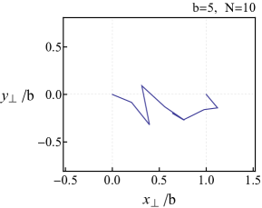
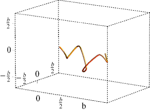
Figure 1: Free transverse string shape at a resolution $x=1/10$ and $b=5$.

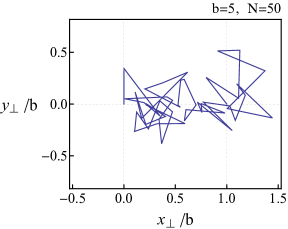
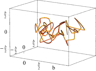
Figure 2: Free transverse string shape at a resolution of $x=1/50$ and $b=5$.

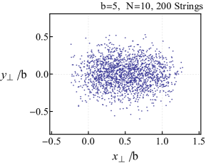
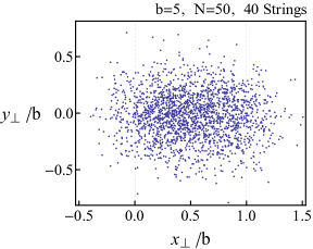
Figure 3: Transverse string bit distributions: at $x=1/10$ sampling 200 strings (${\bf Left}$) and at $x=1/50$ sampling 40 strings (${\bf Right}$).

In its ground state, each of the discretized string bit coordinates $X_{n}^{i}$ is normally distributed with probability $|\Psi(X_{n}^{i})|^{2}$. This gives rise to a random walk of the string bits along the chain in the transverse direction with fixed end-points. This is also true for the continuum. In Fig. 1 and Fig. 2 we show the string shape for a fixed distance ${\bf b}=5$ for two distinct resolutions $N=10$ and $N=50$ respectively. The left figure is the string projected in the transverse plane, while the right figure is the string in $D_{\perp}=3$ dimensions. Fig. 3 (left) show the string bits in the transverse plane for an ensemble of 200 strings at a resolution of $N=10$ with fixed $b=5$. Fig. 3 (right) shows the same for 40 strings at a higher resolution $N=50$.

III Self-interacting string in the Mean-Field Approximation

Attractive string self-interaction will cause the string to shrink transversely, while repulsive self-interactions will cause the transverse string to grow outward, in a way pushing the string bits out. While string bits are held by confinement which is harmonic in our discretized case, self-string interactions are not well-known. We now postulate that for a sufficiently high resolution or large $N$ we may average the inter-bit interactions in the string using two-body self-interactions

$$V=-\frac{g^{2}}{2}\sum_{k\neq k^{\prime}}\int\frac{d^{D_{\perp}+1}p}{(2\pi)^{D_{\perp}+1}}\,\frac{M(\vec{x}_{k})M(\vec{y}_{k})}{p^{2}+m^{2}}\exp\left(i\vec{p}\cdot(\vec{x}_{k}-\vec{y}_{k})\right)$$ (3.0.1)

where $M(\vec{x}_{k})$ is the mass of the discrete point at $\vec{x}_{k}$. Here $m$ is a finite mass in units of the string length that characterizes the range of the interaction. Most of our numerical analyses to follow will be for $m=0$. Results at finite $m$ may be mapped on $m=0$ through a pertinent re-scaling of the bare coupling $g\rightarrow g(m)$. Note that the static interaction involves the virtual exchange in $D_{\perp}+1$ as the holographic set up is in $D_{\perp}+2$. The effect of the curvature of AdS₅ will be assessed phenomenologically below.

In holographic QCD $m$ is typically the mass of the graviton in bulk which is dual to the glueball mass on the boundary. In the large number of colors limit, the value of $m$ is large. However, for a finite number of colors and flavors mixing between the glueballs and the flavor scalars lead to a much lighter $m$ Kalaydzhyan and Shuryak (2014); Liu and Zahed (2014a, b). Also, in a dense but cold gluon medium the glueball mass maybe lighter. In our case we will consider $m$ a parameter that could be re-absorbed by redefining $g$. Throughout we will discuss in detail the attractive self-interactions or $g^{2}>0$. The repulsive case and results will only be quoted. Note that our analysis of the string ground state is quantum so that self-interactions do not result in a string collapse thanks to the quantum uncertainty principle.

For large $N$, the bit coordinates $x_{k}$ and $x_{k^{\prime}}$ are approximately independent. They are normally distributed with a probability distribution

$$\rho(\vec{x}_{k})=\left(\frac{1}{\Sigma_{k}\sqrt{2\pi}}\right)^{D_{\perp}}\exp\left(-\frac{(\vec{x}_{k}-\vec{b}\frac{k}{N})^{2}}{2\Sigma_{k}^{2}}\right)$$ (3.0.2)

The squared variance is

$$\Sigma_{k}^{2}=\sum_{n=1}^{N-1}\frac{\sin^{2}\left(\frac{nk}{N}\pi\right)}{2\omega_{n}}\approx\sum_{n=1}^{N-1}\frac{1}{4\omega_{n}}=\frac{R_{\perp}^{2}}{D_{\perp}}$$ (3.0.3)

We note that the normal frequencies $\omega_{n}$ differ from the free frequencies $\Omega_{n}$. They are defined variationally below. (3.0.1) is a highly simplified two-body interaction as higher-order many-body interactions are also possible. We just note that $g\approx 1/N_{c}$ justifying the dominance of the two-body interactions.

Using (3.0.2) we may define the bit mass distribution on the string in the mean-field type approximation as

$$M(\vec{x}_{k})\approx\frac{M_{\perp}}{N+1}\rho(\vec{x}_{k})$$ (3.0.4)

Inserting (3.0.2-3.0.4) into (3.0.1) yield

$$V=-\frac{g^{2}}{2}\sum_{k\neq k^{\prime}}\left(\frac{M_{\perp}}{N+1}\right)^{2}\int\frac{d^{D_{\perp}+1}p}{(2\pi)^{D_{\perp}+1}}\,\,\rho(\vec{x}_{k})\rho(\vec{y}_{k^{\prime}})\frac{e^{i\vec{p}\cdot\left(\vec{x}_{k}-\vec{y}_{k}\right)}}{p^{2}+m^{2}}$$ (3.0.5)

In the large $N$ limit, we may average (3.0.5) over $x_{k}$ and $y_{k}$ to obtain in the mean-field approximation

$$\overline{V} \equiv -\frac{g^{2}}{2}\sum_{k\neq k^{\prime}}\left(\frac{M_{\perp}}{N+1}\right)^{2}\int d^{D_{\perp}}x_{k}\int d^{D_{\perp}}y_{k}\int\frac{d^{D_{\perp}+1}p}{(2\pi)^{D_{\perp}+1}}\,\,\rho(\vec{x}_{k})\rho(\vec{y}_{k^{\prime}})\frac{e^{i\vec{p}\cdot\left(\vec{x}_{k}-\vec{y}_{k}\right)}}{p^{2}+m^{2}}$$ (3.0.6)

$$= -\frac{g^{2}}{2}\sum_{k\neq k^{\prime}}\left(\frac{M_{\perp}}{N+1}\right)^{2}\int\frac{d^{D_{\perp}+1}p}{(2\pi)^{D_{\perp}+1}}\,\,\frac{1}{p^{2}+m^{2}}\exp\left[-\frac{p^{2}}{2}\left(\Sigma_{k}^{2}+\Sigma_{k^{\prime}}^{2}\right)+i\vec{p}\cdot\vec{b}\frac{(k-k^{\prime})}{N}\right]$$

Thus

$$\overline{V} \approx -\frac{g^{2}}{2}M_{\perp}^{2}\int\frac{d^{D_{\perp}+1}p}{(2\pi)^{D_{\perp}+1}}\,\,\frac{1}{p^{2}+m^{2}}\int_{0}^{1}dk\int_{0}^{1}dk^{\prime}\exp\left[-p^{2}\frac{R_{\perp}^{2}}{D_{\perp}}+i\vec{p}\cdot\vec{b}(k-k^{\prime})\right]$$ (3.0.7)

$$= -\frac{g^{2}}{2}M_{\perp}^{2}\int\frac{d^{D_{\perp}+1}p}{(2\pi)^{D_{\perp}+1}}\,\,\frac{1}{p^{2}+m^{2}}\exp\left(-p^{2}\frac{R_{\perp}^{2}}{D_{\perp}}\right)\frac{4\sin^{2}\left(\frac{\vec{p}\cdot\vec{b}}{2}\right)}{\left(\vec{p}\cdot\vec{b}\right)^{2}}$$

For $m=0$ and $\vec{b}\rightarrow 0$, (3.0.5) simplifies

$$\overline{V}\approx-{\bf C}(D_{\perp})\,g^{2}\,\frac{M^{2}_{\perp}}{R_{\perp}^{D_{\perp}-1}}$$ (3.0.8)

with ${\bf C}\equiv(1/\sqrt{16\pi D_{\perp}})\left(D_{\perp}/4\pi\right)^{\frac{D_{\perp}}{2}}\Gamma(D_{\perp}/2-1/2)/\Gamma(D_{\perp}/2+1/2)$. In this limit, the self-interactions between the string bits reduce to a Newtonian potential acting as a mean-field approximation. The Newtonian constant is identified as $G_{N}=g^{2}D_{\perp}^{(D_{\perp}-1)/2}/(8\pi)$ through the bottom-up holographic setting in $D_{\perp}+2$ dimensions Stoffers and Zahed (2013a). Thus,

$$g^{2}=8\pi D_{\perp}^{\frac{1-D_{\perp}}{2}}\,l_{P}^{D\perp}=8\pi D_{\perp}^{\frac{1-D_{\perp}}{2}}\,g_{s}^{2}l_{s}^{D_{\perp}}\equiv 2^{3-D_{\perp}}\pi D_{\perp}^{\frac{1-D_{\perp}}{2}}\,g_{s}^{2}$$ (3.0.9)

where in the last equality we reset $2l_{s}\equiv 1$ as per our current conventions. Recall that the curvature effects of AdS₅, which we are ignoring so far, amounts to an effective $D_{\perp}\rightarrow D_{\perp}(\lambda)$ in leading order on the transverse string propagator as we noted earlier. This observation will be used below to estimate the curvature corrections to the current analysis.

IV Variational Analysis

For small perturbative interactions, we can modify the transverse Hamiltonian through

$$\mathcal{H}_{\perp}=2M_{\perp}^{2}+2M_{\perp}\delta(2M_{\perp})\equiv 2M_{\perp}^{2}+2M_{\perp}\,\overline{V}$$ (4.0.1)

$\mathcal{H}_{\perp}$ in Eq. 4.0.1 is difficult to analyze analytically in the presence of $\overline{V}$. We follow Thorn and Ogerman Bergman and Thorn (1997) and analyze it variationally by using a trial Gaussian distribution for each string bit

$$\Psi(X_{n}^{i})=\left(\frac{\omega_{n}}{\pi}\right)^{\frac{1}{4}}\exp\left[-\frac{\omega_{n}}{2}(X_{n}^{i})^{2}\right]$$ (4.0.2)

where the set of normal modes $\omega_{n}$ will be defined below by minimizing the energy of the string in the presence of $V$. In terms of (4.0.2) the scalar part is

$$\mathcal{H}_{\perp}^{0}=\frac{D_{\perp}}{4}\sum_{n=1}^{N-1}\left(\omega_{n}+\frac{\Omega_{n}^{2}}{\omega_{n}}\right)+\frac{b^{2}}{\pi^{2}}$$ (4.0.3)

and reduces to (2.0.10) when $\omega_{n}=\Omega_{n}$ for $V=0$. The effective mass of the string is

$$M_{\perp}^{2}[\omega_{n}]=\frac{1}{2}\mathcal{H}_{\perp}^{0}=\frac{D_{\perp}}{8}\sum_{n=1}^{N-1}\left(\omega_{n}+\frac{\Omega_{n}^{2}}{\omega_{n}}\right)+\frac{b^{2}}{2\pi^{2}}$$ (4.0.4)

The squared effective transverse radius is

$$R_{\perp}^{2}[\omega_{n}]=\frac{1}{N}\sum_{k=0}^{N}\left<\left(x_{k}^{i}-\mathbb{b}^{i}\frac{k}{N}\right)^{2}\right>=\frac{D_{\perp}}{4}\sum_{n=1}^{N-1}\frac{1}{\omega_{n}}$$ (4.0.5)

With our conventions the total string energy is $E[\omega_{n}]=2M_{\perp}^{2}+2M_{\perp}\overline{V}$ depends on the set of variational parameters $\omega_{n}$ which are fixed through the minimum

$$\frac{\delta E}{\delta\omega_{n}} = \frac{\delta M_{\perp}^{2}}{\delta\omega_{n}}\left[2-\frac{3g^{2}}{2}M_{\perp}\int\frac{d^{D_{\perp}+1}p}{(2\pi)^{D_{\perp}+1}}\,\,\frac{1}{p^{2}+m^{2}}\exp\left(-p^{2}\frac{R_{\perp}^{2}}{D_{\perp}}\right)\frac{4\sin^{2}\left(\frac{\vec{p}\cdot{b}}{2}\right)}{\left(\vec{p}\cdot\vec{b}\right)^{2}}\right]$$ (4.0.6)

$$+\frac{1}{D_{\perp}}\frac{\delta R_{\perp}^{2}}{\delta\omega_{n}}g^{2}M_{\perp}^{3}\int\frac{d^{D_{\perp}+1}p}{(2\pi)^{D_{\perp}+1}}\,\,\frac{p^{2}}{p^{2}+m^{2}}\exp\left(-p^{2}\frac{R_{\perp}^{2}}{D_{\perp}}\right)\frac{4\sin^{2}\left(\frac{\vec{p}\cdot{b}}{2}\right)}{\left(\vec{p}\cdot\vec{b}\right)^{2}}=0$$

The mass and size variations can be made explicit

$$\frac{\delta M_{\perp}^{2}}{\delta\omega_{n}}=\frac{D_{\perp}}{8}\left(1-\frac{\Omega_{n}^{2}}{\omega_{n}^{2}}\right)\ \ \ \ \ \ \ \ \ \ \frac{1}{D_{\perp}}\frac{\delta R_{\perp}^{2}}{\delta\omega_{n}}=-\frac{1}{4\omega_{n}^{2}}$$ (4.0.7)

Inserting (4.0.7) into (4.0.6) and rearranging yield

$$\omega_{n}^{2}=\Omega_{n}^{2}+\frac{\frac{g^{2}M_{\perp}^{3}}{D_{\perp}}\int\frac{d^{D_{\perp}+1}p}{(2\pi)^{D_{\perp}+1}}\,\,\frac{p^{2}}{p^{2}+m^{2}}\exp\left(-p^{2}\frac{R_{\perp}^{2}}{D_{\perp}}\right)\frac{4\sin^{2}\left(\frac{\vec{p}\cdot{b}}{2}\right)}{\left(\vec{p}\cdot\vec{b}\right)^{2}}}{1-\frac{3g^{2}}{4}M_{\perp}\int\frac{d^{D_{\perp}+1}p}{(2\pi)^{D_{\perp}+1}}\,\,\frac{1}{p^{2}+m^{2}}\exp\left(-p^{2}\frac{R_{\perp}^{2}}{D_{\perp}}\right)\frac{4\sin^{2}\left(\frac{\vec{p}\cdot{b}}{2}\right)}{\left(\vec{p}\cdot\vec{b}\right)^{2}}}$$ (4.0.8)

where both $M^{2}_{\perp}[\omega_{n}]$ and $R_{\perp}^{2}[\omega_{n}]$ depend on the variational parameters through (4.0.4-4.0.5). (4.0.8) define a highly non-linear set of equations for the variational parameters $\omega_{n}$ defining the Gaussian ansatz (4.0.2). The generic solution is of the form $\omega_{n}=\sqrt{\Omega_{n}^{2}+\eta^{2}}$ with

$$\eta^{2}=\frac{\frac{g^{2}M_{\perp}^{3}}{D_{\perp}}\int_{0}^{\infty}dp\int_{0}^{\pi}d\phi\,\,\left(\sin\phi\right)^{D_{\perp}-1}\frac{p^{D_{\perp}+2}}{p^{2}+m^{2}}\exp\left(-p^{2}\frac{R_{\perp}^{2}}{D_{\perp}}\right)\frac{4\sin^{2}\left(\frac{pb\cos\phi}{2}\right)}{p^{2}b^{2}\cos^{2}\phi}}{2^{D_{\perp}}\pi^{\frac{D_{\perp}+2}{2}}\Gamma(\frac{D_{\perp}}{2})-\frac{3g^{2}}{4}M_{\perp}\int_{0}^{\infty}dp\int_{0}^{\pi}d\phi\,\,\left(\sin\phi\right)^{D_{\perp}-1}\frac{p^{D_{\perp}}}{p^{2}+m^{2}}\exp\left(-p^{2}\frac{R_{\perp}^{2}}{D_{\perp}}\right)\frac{4\sin^{2}\left(\frac{pb\cos\phi}{2}\right)}{p^{2}b^{2}\cos^{2}\phi}}$$ (4.0.9)

to be determined numerically. Note that for $b=0$, (4.0.9) simplifies as

$$\eta^{2}=\frac{M_{\perp}^{2}}{R_{\perp}^{2}}\frac{\frac{1}{2}\frac{g^{2}M_{\perp}}{R_{\perp}^{D_{\perp}-1}}\exp\left(\frac{m^{2}R_{\perp}^{2}}{D_{\perp}}\right)\Gamma\left(\frac{3+D_{\perp}}{2}\right)\left(\frac{m^{2}R_{\perp}^{2}}{D_{\perp}}\right)^{\frac{D_{\perp}+1}{2}}\Gamma\left(-\frac{1+D_{\perp}}{2},\frac{m^{2}R^{2}}{D_{\perp}}\right)}{2^{D_{\perp}}\pi^{\frac{D_{\perp}+1}{2}}\left(D_{\perp}\right)^{\frac{1-D_{\perp}}{2}}\Gamma(\frac{D_{\perp}+1}{2})-\frac{3}{8}\frac{g^{2}M_{\perp}}{R_{\perp}^{D_{\perp}-1}}\exp\left(\frac{m^{2}R_{\perp}^{2}}{D_{\perp}}\right)\Gamma\left(\frac{1+D_{\perp}}{2}\right)\left(\frac{m^{2}R_{\perp}^{2}}{D_{\perp}}\right)^{\frac{D_{\perp}-1}{2}}\Gamma\left(-\frac{D_{\perp}-1}{2},\frac{m^{2}R^{2}}{D_{\perp}}\right)}$$

(4.0.10)

For $m=0$, Eq. 4.0.10 further simplifies as

$$\eta^{2}=\frac{M_{\perp}^{2}}{R_{\perp}^{2}}\frac{\frac{1}{2}\frac{g^{2}M_{\perp}}{R_{\perp}^{D_{\perp}-1}}}{2^{D_{\perp}}\pi^{\frac{D_{\perp}+1}{2}}\left(D_{\perp}\right)^{\frac{1-D_{\perp}}{2}}-\frac{3}{4(D_{\perp}-1)}\frac{g^{2}M_{\perp}}{R_{\perp}^{D_{\perp}-1}}}$$ (4.0.11)

Note that for $b\neq 0$, (4.0.9) simplifies as

$$\eta^{2}=\frac{M_{\perp}^{2}}{b^{2}}\frac{\frac{4}{D_{\perp}}\frac{g^{2}M_{\perp}}{b^{D_{\perp}-1}}{\bf I}[0]}{2^{D_{\perp}}\pi^{\frac{D_{\perp}+2}{2}}\Gamma(\frac{D_{\perp}+1}{2})-3\frac{g^{2}M_{\perp}}{b^{D_{\perp}-1}}{\bf I}[2]}$$ (4.0.12)

where

$${\bf I}[a]\equiv\int_{0}^{\infty}dx\int_{0}^{\pi}d\phi\,\,\left(\sin\phi\right)^{D_{\perp}-3}\tan^{2}\phi\,\,\frac{x^{D_{\perp}-a}}{x^{2}+m^{2}b^{2}}\exp\left(-\frac{x^{2}}{D_{\perp}}\frac{R_{\perp}^{2}}{b^{2}}\right)\sin^{2}\left(\frac{x\cos\phi}{2}\right)$$ (4.0.13)

The repulsion will cause the string bits to expand. A rerun of the precedent arguments yields now $\omega_{n}=\sqrt{\Omega_{n}^{2}-\eta^{2}}$ with

$$\eta^{2}=\frac{M_{\perp}^{2}}{b^{2}}\frac{\frac{4}{D_{\perp}}\frac{\tilde{g}^{2}M_{\perp}}{b^{D_{\perp}-1}}{\bf I}[0]}{2^{D_{\perp}}\pi^{\frac{D_{\perp}+2}{2}}\Gamma(\frac{D_{\perp}+1}{2})+3\frac{\tilde{g}^{2}M_{\perp}}{b^{D_{\perp}-1}}{\bf I}[2]}$$ (4.0.14)

The variational analysis will be now carried numerically for both the attractive and repulsive string interaction in the mean-field approximation.

V Numerical Results

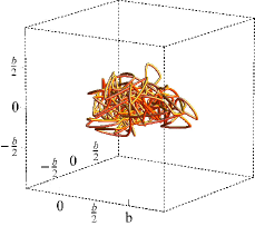
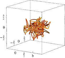
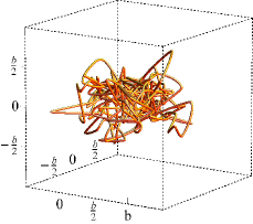
Figure 4: Attractive interaction: $g=0.3$ ($\mathbb{Left}$).    No interaction: $g=\tilde{g}=0$ ($\mathbb{Center}$).    Repulsive interaction: $\tilde{g}=0.3$ ($\mathbb{Right}$).

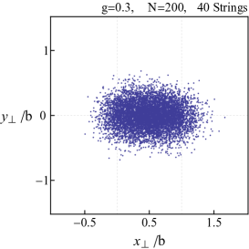
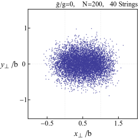
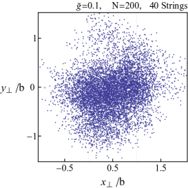
Figure 5: Attractive interaction: $g=0.3$ ($\mathbb{Left}$).    No interaction: $g=\tilde{g}=0$ ($\mathbb{Center}$).    Repulsive interaction: $\tilde{g}=0.1$ ($\mathbb{Right}$).

The Gaussian variation ansatz (4.0.2) can be used to define a variational probability distribution $|\Psi(X_{n}^{i})|^{2}$ for the string amplitudes $X_{n}^{i}$ in the normal mode decomposition (10.0.4). Each string bit undergoes a Gaussian random walk which is free for $g=0$ but constrained by the interaction through $\omega_{n}$ for $g\neq 0$. In Fig. 4 we show the spatial geometry of our discretized strings in $D_{\perp}=3$ with a resolution $N=200$ for the attractive interaction $g=0.3$, no interaction and repulsive interaction $\tilde{g}=0.3$. The string is stretched with $b=5$. In Fig. 5 we show the transverse distribution of the string bits for an ensemble consisting of 40 stretched strings. The string bits are the dots and we have left out the string connection for a better visualization. The resolution is $N=1/x=200$. The attractive configurations are denser along $b$, while the repulsive configurations are spread out of $b$.

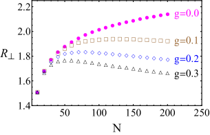
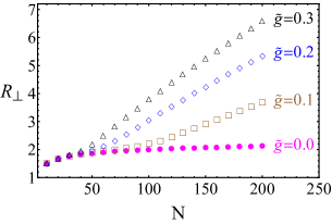
Figure 6: Attractive interaction: $g=0.1,0.2,0.3$ ($\mathbb{Left}$).    Repulsive interaction: $\tilde{g}=0.1,0.2,0.3$ ($\mathbb{Right}$).

In Fig. 6 we show the growth of the transverse radius as measured by (4.0.5) versus the resolution $N$ for different strengths of the attractive forces (left) and repulsive forces (right). For comparison, we also show the full length of the string

$$L\equiv\sum_{k=1}^{N}\sqrt{\left(x_{k}^{i}-x_{k-1}^{i}\right)^{2}}$$ (5.0.1)

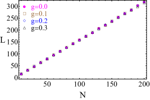
Figure 7: Attractive interaction: $g=0.1,0.2,0.3$ ($\mathbb{Left}$).    Repulsive interaction: $\tilde{g}=0.1,0.2,0.3$ ($\mathbb{Right}$).

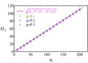
Figure 8: Solid line is the analytical result in (2.0.14). Numeric datas are for attractive interaction: $g=0.1,0.2,0.3$ ($\mathbb{Left}$) and repulsive interaction: $\tilde{g}=0.1,0.2,0.3$ ($\mathbb{Right}$).

The analogue change of the total length of the string with the resolution as defined in (5.0.1) and the mass of the string as defined in (4.0.4) are also shown in Fig. 7 and Fig. 8. While the length and mass scale linearly with $N$ whatever the interaction, the transverse size of the string bit distribution shows sensitivity to $N$. For $g=\tilde{g}=0$ the transverse radius grows logarithmically as expected. As the attraction is switched on, the transverse radius asymptotes a constant about the string length. In contrast, as the repulsion is switched on, the transverse radius asymptotes a linear rise with the resolution as also noted in Bergman and Thorn (1997) in their non-relativistic string bit models with a variety of repulsive string interactions of different ranges. This supports our earlier earlier observation that at large resolution $N$ the mean-field approximation is generic.

We note that all attractive string self-interactions result in transverse area that are less than or equal to the Froissart bound. In contrast, all repulsive string self-interactions result in a transverse area that upsets the Froissart bound at asymptotic $N$ or asymptotically low-x. Thus our observation that saturation of the Bekenstein bound by the the string bits or wee gluons, follows from weakly attractive string-self interactions in conformity with the Froissart bound. We also note that our treatment of the interaction assumes weak self-interactions, or the smallness of the ratio

$$\frac{2M_{\perp}\overline{V}}{\mathcal{H}_{\perp}^{0}}=\frac{\overline{V}[g]}{M_{\perp}[g]}$$ (5.0.2)

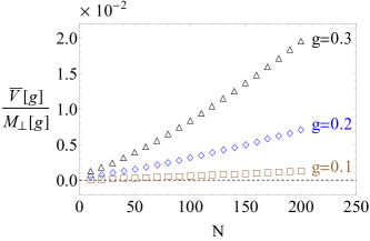
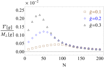
Figure 9: Attractive interaction: $g=0.1,0.2,0.3$ ($\mathbb{Left}$).    Repulsive interaction: $\tilde{g}=0.1,0.2,0.3$ ($\mathbb{Right}$).

We show in Fig. 9 that this is indeed the case.

VI Saturation

At low-x or large $N$ and $b=0$, the transverse string density is high ${\bf n}_{\perp}(0,N)\approx N/R_{\perp}^{D_{\perp}}$ as $R_{\perp}$ shrinks under the effect of attractive self-interactions. For $0<g<0.3$ our numerical results yield $1.2<R_{\perp}<1.6$ in units where $2l_{s}=1$, i.e. $2.4<R_{\perp}/l_{s}<3.2$. To understand the effects of the self-interaction on the string size configuration, we re-write schematically the squared mass $E=2M_{\perp}^{2}+2M_{\perp}V$ of the self-interacting string in terms of $N$ and $R_{\perp}$ dropping all numerical factors

$$E\approx N^{2}\frac{1}{R_{\perp}^{2}}+N^{2}\frac{R_{\perp}^{2}}{D^{2}_{\perp}{{\rm ln}^{2}N}}-N^{2}\frac{g^{2}N}{R_{\perp}^{D_{\perp}-1}}$$ (6.0.1)

The first contribution in (6.0.1) follows from the kinetic contribution in (2.0.6) using the estimate $N^{2}p_{i}^{2}$ and the uncertainty principle $p_{i}\approx 1/R_{\perp}$. The second contribution in (6.0.1) follows from the harmonic potential in (6.0.1) using the estimate $N^{2}(\Delta x_{i})^{2}$ with typically $\Delta x_{i}\approx R_{\perp}/(D_{\perp}{\rm ln}N)$ in the diffusive regime. The third contribution in (6.0.1) is the potential contribution $2M_{\perp}\,\overline{V}$ to the squared mass after using $M_{\perp}\approx N$. Note that for $g=0$ the minimum of (6.0.1) yields the diffusive result $R^{2}_{\perp}\approx D_{\perp}{{\rm ln}N}$ whatever $D_{\perp}$. For finite $g$, the minimum of (6.0.1) depends on the dimensionality $D_{\perp}$. A similar relation to (6.0.1) was found to hold for classical strings at hi high temperature by Damour and Veneziano Damour and Veneziano (2000) using different arguments.

VI.1 Flat Space: $D_{\perp}=3$

For our case $D_{\perp}=3$ so the minimum of (6.0.1) occurs for

$$R_{\perp}\approx\left(1-g^{2}N\right)^{1/4}\,\sqrt{{\rm ln}N}$$ (6.1.2)

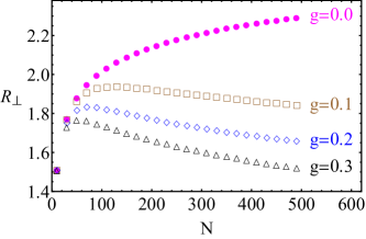
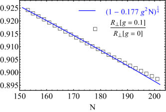
Figure 10: $R_{\perp}[g]$ for $g=0.1,0.2,0.3$ $(\mathbb{Left})$.      $R_{\perp}[g=0.1]/R_{\perp}[g=0]$ for large $N$ $(\mathbb{Right})$.

For a relatively small attraction $g^{2}N\approx 1$, $R_{\perp}$ in (6.1.2) undergoes a numerical change from an increasingly large and diffusive string to a small and fixed size string of about few string lengths. Fig. 10 (left) shows that for $g=0.1$ the transverse size flattens out at about $R_{\perp}\sim 1.85\equiv 3.7l_{s}\approx 0.3$ fm in the range $200<N<600$. For fixed $b$ the transverse area is ellipsoidal with a transverse bit density

$${\bf n}_{\perp}(b,N)\approx\frac{N}{b\left(2R_{\perp}\right)^{D_{\perp}-1}}\equiv\frac{N}{N_{c}}\frac{1}{g^{2}l_{s}^{D_{\perp}}}\frac{g^{2}N_{c}}{\frac{b}{l_{s}}\left(2\frac{R_{\perp}}{l_{s}}\right)^{D_{\perp}-1}}$$ (6.1.3)

The critical resolution $x_{c}=1/N_{c}$ at which this change takes place can be read from Fig. 10 (right)

$$x_{c}=\frac{1}{N_{c}}\approx 0.1^{2}\times 0.177=1.77\times 10^{-3}$$ (6.1.4)

for $g=0.1$ with $D_{\perp}=3$ and $b=5\equiv 10\,l_{s}\approx 1$ fm. We identify the onset $x\approx x_{c}$ as the pre-saturation phase of the string at high resolution whereby its transverse area contracts to the string scale under weak self-attraction. However, the transverse string bit density is still dilute at this resolution since

$${\bf n}_{\perp}(5,x)\approx\frac{x_{c}}{x}\frac{1}{\frac{\pi}{3}l_{p}^{3}}\frac{1}{10\times\left(4\times 1.85\right)^{2}\times 0.177}=\frac{x_{c}}{x}\frac{0.01}{l_{p}^{3}}\equiv\frac{x_{s}}{x}\frac{1}{l_{p}^{3}}$$ (6.1.5)

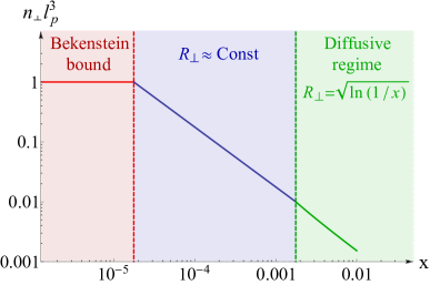
Figure 11: Saturation (red), pre-saturation (blue) and diffusive (green) regimes for a transverse string with decreasing resolution in $D_{\perp}=3$. See text.

or $n_{\perp}(5,x_{c})\approx 0.01/l_{P}^{3}$. Recall that the Planck length $l_{P}^{D_{\perp}}=g_{s}^{2}l_{s}^{D_{\perp}}$ and that $g^{2}=(\pi/3)g_{s}^{2}$ from (3.0.9). At the saturation point or $x\equiv x_{s}=0.01x_{c}\approx 10^{-5}$ the transverse density saturates the Bekenstein bound of one bit per transverse Planck area or $n_{\perp}(5,x_{s})\approx 1/l_{P}^{3}$. We identify this point with the saturation scale or black hole regime. A schematic rendering of the pre-saturation and saturation phases in the low-x regime for $b=5$ are shown in Fig. 11.

VI.2 Curved Space: $D_{\perp}(\lambda)<3$

An exact spatial analysis of the transverse string in curved AdS₅ space is beyond the scope of this work. In this section we will attempt to give simple estimates of the effects of the curvature of AdS₅ on some of our previous results. For that we first note that an aspect of the curved geometry on the Pomeron is to cause the string transverse degrees of freedom to effectively feel a reduced transverse spatial dimension  Stoffers and Zahed (2013a); Stoffers and Zahed (2012); Stoffers and Zahed (2013b); Shuryak and Zahed (2014)

$$D_{\perp}\rightarrow D_{\perp}(\lambda)=D_{\perp}\left(1-\frac{3(D_{\perp}-1)^{2}}{2D_{\perp}\sqrt{\lambda}}+{\cal O}\left(\frac{1}{\lambda}\right)\right)$$ (6.2.6)

with $\lambda=g^{2}_{YM}N_{c}$. Indeed, (6.2.6) causes the Pomeron intercept to move from $D_{\perp}/12=0.25$ to $D_{\perp}(\lambda\approx 40)\approx 0.17$ closer to the empirical interceptt of $0.08$ Donnachie and Landshoff (1992). A phenomenological way to implement this effect is to add warping factors on the oscillators in (2.0.1) as we detail in the Appendix and repeat the numerical analysis. A simpler estimate follows from the substitution (6.2.6) in the interacting part of our variational analysis. Indeed, the schematic estimate (6.0.1) shows that the first contribution reflects on the uncertainty principle which probes short distances and thus is not sensitive to the curvature of AdS₅. The second diffusive contribution is sensitive through $D_{\perp}$ but will turn out to be subleading as we will show below. The third contribution is long ranged and senses the curvature of AdS₅. Thus

$$E\rightarrow N^{2}\frac{1}{R_{\perp}^{2}}+N^{2}\frac{R_{\perp}^{2}}{D_{\perp}^{2}(\lambda)\,{{\rm ln}^{2}N}}-N^{2}\frac{g^{2}N}{R_{\perp}^{D_{\perp}(\lambda)-1}}$$ (6.2.7)

For very small values of $g$ the first two contributions in (6.2.7) are dominant and the string transverse size grows diffusively. The minimization of the first two dominant contributions in this regime yields $R^{2}_{\perp}\approx D_{\perp}(\lambda)\,{\rm ln}N$. This is consistent with the growth of the Pomeron in curved AdS₅ noted in Stoffers and Zahed (2013a); Stoffers and Zahed (2012); Stoffers and Zahed (2013b); Shuryak and Zahed (2014). However, for

$$g^{2}>\frac{1}{N}\left(\ln N\right)^{\frac{D_{\perp}(\lambda)-3}{2}}$$ (6.2.8)

the string size shrinks and the transverse string size follows from balancing the first term with the last term due to the interaction. The balance between the self-interaction and the uncertainty principle, yields a continuously decreasing transverse string size

$$R_{\perp}\approx\left(\frac{1}{g^{2}N}\right)^{\frac{2\sqrt{\lambda}}{3(D_{\perp}-1)^{2}}}$$ (6.2.9)

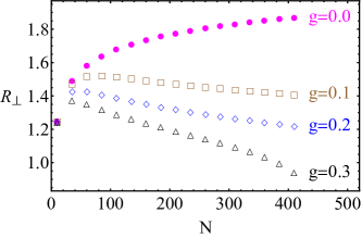
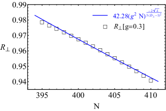
Figure 12: $R_{\perp}[g]$ for $g=0.1,0.2,0.3$ $(\mathbb{Left})$.            $R_{\perp}[g=0.3]$ and Eq. 6.2.9 $(\mathbb{Right})$.

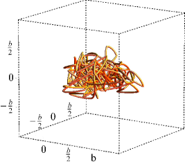
Figure 13: 3D configuration of the string with $N=200$ and $g=0.3$ using $D_{\perp}(\lambda)$ in the interaction. See text.

in units of the string length. A typical configuration of the string with $N=200$ using the string interaction (3.0.5-3.0.7) with the effective substitution $D_{\perp}\rightarrow D_{\perp}(\lambda)$ is displayed in Fig. 13. For $\lambda=40$, $D_{\perp}=3$ and $g=0.3$, the scaling regime (6.2.9) is observed to take place for our string samplings for $N_{c}\approx 400$ as shown in Fig. 12. As before, we identify the critical resolution $x_{c}=1/N_{c}\approx 0.0025$ with the onset of the scaling regime (6.2.9).

The transverse density for fixed impact parameter $b$ is now

$${\bf n}_{\perp}(b,x=1/N)\approx\frac{N}{b\left(2R_{\perp}\right)^{{D_{\perp}}-1}}\approx\left({\frac{(0.3)^{2}\times 400}{x/x_{c}}}\right)^{\frac{2\sqrt{\lambda}}{3(D_{\perp}-1)}+1}\left(\frac{l_{s}}{b}\right)\left(\frac{1}{2\times 42.28}\right)^{D_{\perp}-1}\,\frac{1}{l_{p}^{{D_{\perp}}}}$$ (6.2.10)

For a typical impact parameter of $b=5l_{s}$, it saturates the Bekenstein bound for $x\equiv x_{s}\approx 0.6x_{c}$ ($1/x_{s}=N_{s}\approx 633$)

$${\bf n}_{\perp}(5,x_{s}\approx 0.0016)\approx\frac{1}{l_{p}^{{D_{\perp}}}}$$ (6.2.11)

In Fig. 14 we give a schematic rendering of the diffusive (green, pre-saturation (blue) and saturation (red) regimes foliowing from the effective $D_{\perp}\rightarrow D_{\perp}(\lambda)$ substitution.

VI.3 Stringy Saturation

In flat $D_{\perp}=3$ the transverse string size distribution remains diffusive or logarithmic in $N$ for small self-attractive interactions in the range $0<g^{2}N<1$. However for $g^{2}N\approx 1-1/{\rm ln}^{2}N$ the transverse string size shrinks to a fixed size comparable to the string length. The change sets in at weak coupling with $g^{2}\approx 1/N$, for which the transverse density at $b=0$ is now

$${\bf n}_{\perp}(0,x=1/N)\approx\frac{N}{R_{\perp}^{D_{\perp}}}\rightarrow{(g^{2}N)}\frac{1}{l_{p}^{D_{\perp}}}$$ (6.3.12)

after restoring the string length. The first transition occurs in a very narrow range of $g$ and thus appears to be first order by our analysis in (6.0.1-6.1.2). It is a pre-saturation transition where the string size shrinks away from its diffusive growth and remains about fixed at a relatively dilute transverse string bit density. At much higher resolution or low-x a saturation transition takes place when the transverse string bit distribution reaches the Bekenstein bound of one string bit per Planck scale. This maybe intuitively understood by noting that low-x follows from large boosts a situation analogous to falling matter on a black-hole. For completeness, we note that self-repulsive strings increase in sizes following the substitution $g^{2}\rightarrow-g^{2}$ in (6.3.12).

Using the estimates for the AdS curvature through the substitution (6.2.6) yields

$${\bf n}_{\perp}(0,x=1/N)\approx\frac{N}{R_{\perp}^{{D_{\perp}}}}\longrightarrow\left(g^{2}N\right)^{\frac{2\sqrt{\lambda}D_{\perp}}{3(D_{\perp}-1)^{2}}}\frac{1}{l_{p}^{D_{\perp}}}$$ (6.3.13)

instead of (6.3.12). (6.3.13) reaches more smoothly the Bekenstein bound as the string self-interaction satisfies $g^{2}N\approx 1$. Alternatively, the effective density using the effective dimension $D_{\perp}(\lambda)$

$$\tilde{\bf n}_{\perp}(0,x=1/N)\approx\frac{N}{R_{\perp}^{{D_{\perp}}(\lambda)}}\rightarrow\left({g^{2}N}\right)^{\frac{2\sqrt{\lambda}D_{\perp}(\lambda)}{3(D_{\perp}-1)^{2}}+\frac{D_{\perp}(\lambda)}{D_{\perp}}}\,\left(\frac{1}{x}\right)^{\frac{3(D_{\perp}-1)^{2}}{2D_{\perp}\sqrt{\lambda}}}\,\frac{1}{l_{p}^{{D_{\perp}}(\lambda)}}$$ (6.3.14)

is seen to increase beyond the Bekenstein bound as the string self-interaction reaches $g^{2}N\approx 1$. There is no black-hole to saturate in fractional dimension.

VI.4 Relation to Saturation in DIS

The present observations on stringy saturation are consistent with the arguments presented in Stoffers and Zahed (2013a); Stoffers and Zahed (2012); Stoffers and Zahed (2013b) whereby the stringy but eikonalized dipole-dipole cross section was found to saturate in the impact parameter space when $g_{s}^{2}l_{s}^{D_{\perp}}n_{\perp}\equiv l_{P}^{D_{\perp}}n_{\perp}\approx 1$ (see their Eq. 47). Although the relationship between the string coupling and the gauge coupling depends on the holographic extension of QCD used, for the generic model of AdS₅ with a wall $g_{s}\approx C\,g^{2}_{YM}/4\pi\equiv C\,\alpha_{s}$ ($C=1$ for AdS₅ without a wall). Our numerical analysis puts $g_{s}\approx 0.1-0.3$.

The 3-dimensional density $n_{\perp}$ was physically interpreted in Stoffers and Zahed (2013a); Stoffers and Zahed (2012); Stoffers and Zahed (2013b) as the number of wee dipoles per unit transverse 2-dimensional space per unit dipole size $z$ along the holographic direction. The latter enforces hyperbolic evolution of the dipole size through the AdS₅ metric (with a wall). At saturation $z_{s}\approx 1/Q_{s}$. The transverse 2-dimensional density is then defined as $Q_{s}^{2}\equiv z_{s}n_{\perp}$.

For curved AdS₅, the Pomeron intercept is $D_{\perp}(\lambda\approx 40)/12\approx=0.17$, and (6.3.13) at saturation gives $l_{s}Q_{s}\approx l_{s}/l_{p}\approx 1/x^{\frac{1}{3}}$. This is to be compared with $l_{s}Q^{GW}_{s}\approx l_{s}/l_{p}\approx 1/x^{0.144}$ obtained empirically by Golec-Wustoff Golec-Biernat and Wusthoff (1998, 1999), and $l_{s}Q^{SZ}_{s}\approx l_{s}/l_{p}\approx 1/x^{0.114}$ obtained by Stoffers and one of us Stoffers and Zahed (2013a); Stoffers and Zahed (2012); Stoffers and Zahed (2013b). For curved $D_{\perp}(\lambda)$, (6.3.14) yields at saturation

$$l_{p}Q_{s}(\lambda)\approx\left(\frac{1}{x}\right)^{\frac{3(D_{\perp}-1)^{2}}{2D_{\perp}\sqrt{\lambda}D_{\perp}(\lambda)}}\rightarrow\left(\frac{1}{x}\right)^{0.155}$$ (6.4.15)

using $D_{\perp}=3$ and $\lambda\approx 40$ Stoffers and Zahed (2013a); Stoffers and Zahed (2012); Stoffers and Zahed (2013b). (6.4.15) is overall consistent with the full AdS₅ curved analysis carried in Stoffers and Zahed (2013a); Stoffers and Zahed (2012); Stoffers and Zahed (2013b), and remarkably close to the empirical result  Golec-Biernat and Wusthoff (1998, 1999).

The saturation of the Bekenstein bound maybe viewed as the string dual to the gluon saturation description in the color glass condensate model for fixed impact parameter using the Pomeron or string slope as a scale Rezaeian et al. (2013); Kowalski and Teaney (2003). The large string bit density (6.3.12) may upset the integrity of the string. Perhaps a more appropriate description is in terms of a fluid of string bits. However, three generic stringy ingredients need to be retained: 1) the string provides for a key property of the wee partons namely their transverse (Gribov) diffusion with a diffusion constant ${\bf D}=l_{s}^{2}/2$ set by the string length; 2) the exponential rise in the string density of states with its mass, provides for the most efficient mechanism to scramble information and reach the Bekenstein bound and thus saturation; 3) the self-interacting string in the mean-field approximation maybe the dual of a Pomeron branching into multiple Pomerons or fan-diagrams in Reggeon calculus Gribov (2003).

VII Angular Deformations

The fluctuating string with fixed end-points exhibit azimuthal deformations in the transverse plane that can be characterized by the azimuthal moment Bzdak et al. (2014); Kalaydzhyan and Shuryak (2014)

$$\epsilon_{n}=\frac{\frac{1}{N}\sum_{i}^{N}e^{in\phi_{i}}\left(r^{\perp}_{i}\right)^{n}}{r_{\perp}^{n}}$$ (7.0.1)

where

$$r_{\perp}^{n}=\frac{1}{N}\sum_{i}^{N}\left(r^{\perp}_{i}\right)^{n}$$ (7.0.2)

with $\phi$ the azimuthal angle as measured from the impact parameter line along ${\bf b}$. $r_{\perp}$ is the averaged size of the string on the transverse plane. For $b=0$, we have $\left<r_{\perp}^{2}\right>/2=R_{\perp}^{2}/D_{\perp}$, where $\left<\cdots\right>$ is the average over string ensembles. Specifically, define $x\equiv x_{\perp}^{i=1}$ and $y\equiv x_{\perp}^{i=2}$ in the transverse plane, where $x$ is parallel to the impact parameter $\mathbb{b}$ and $y$ perpendicular to it,

$$x_{\perp}(k,\tau) = \sum_{n=1}^{N-1}X_{n}(\tau)\sin\left(\frac{nk}{N}\pi\right)+b\frac{k}{N}$$

$$y_{\perp}(k,\tau) = \sum_{n=1}^{N-1}Y_{n}(\tau)\sin\left(\frac{nk}{N}\pi\right)$$ (7.0.3)

Both $X_{n},Y_{n}$ are normally distributed with width $1/2\omega_{n}$ (4.0.2) or

$$X_{n}\sim\mathcal{N}\left(0,\frac{1}{2\omega_{n}}\right)\ \ \ \ \ \ \ \ \ \ \ \ Y_{n}\sim\mathcal{N}\left(0,\frac{1}{2\omega_{n}}\right)$$ (7.0.4)

satisfy the normal distributions. We obtain

$$x_{\perp}(k,\tau)\sim\mathcal{N}\left(b\frac{k}{N},\Sigma_{k}^{2}\right)\ \ \ \ \ \ \ \ \ \ \ \ y_{\perp}(k,\tau)\sim\mathcal{N}\left(0,\Sigma_{k}^{2}\right)$$ (7.0.5)

where

$$\Sigma_{k}^{2}=\sum_{n=1}^{N-1}\frac{\sin^{2}\left(\frac{nk}{N}\pi\right)}{2\omega_{n}}$$ (7.0.6)

For large $N$, each of the transverse coordinates $x_{\perp}(k,\tau)$ are almost independent. The azimuthal moments averaged over the independent transverse coordinates read

$$\left<\epsilon_{n}\right> = \frac{1}{\left<r_{T}^{n}\right>}\left[\frac{1}{N+1}\sum_{k=1}^{N-1}\int_{0}^{\infty}dr\int_{0}^{2\pi}d\phi~{}r^{n+1}\cos(n\phi)~{}\rho\left(r\cos\phi+\frac{b}{2},r\sin\phi,k\right)+\frac{1+(-1)^{n}}{N+1}\left(\frac{b}{2}\right)^{n}\right]$$ (7.0.7)

$$+\frac{i}{\left<r_{T}^{n}\right>}\frac{1}{N+1}\sum_{k=1}^{N-1}\int_{0}^{\infty}dr\int_{0}^{2\pi}d\phi~{}r^{n+1}\sin(n\phi)~{}\rho\left(r\cos\phi+\frac{b}{2},r\sin\phi,k\right)$$

where

$$\left<r_{T}^{n}\right>=\frac{1}{N+1}\sum_{k=1}^{N-1}\int_{0}^{\infty}dr\int_{0}^{2\pi}d\phi~{}r^{n+1}~{}\rho\left(r\cos\phi+\frac{b}{2},r\sin\phi,k\right)+\frac{2}{N+1}\left(\frac{b}{2}\right)^{n}$$ (7.0.8)

and

$$\rho(x,y,k)=\frac{1}{2\pi}\frac{1}{\Sigma_{k}^{2}}\exp\left[-\frac{\left(x-b\frac{k}{N}\right)^{2}+y^{2}}{2\Sigma_{k}^{2}}\right]$$ (7.0.9)

The Gaussian integrations can be done leading to

$$\left<\epsilon_{n}\right>=\frac{b^{n}}{\left<r_{T}^{n}\right>}\left[\frac{1}{N+1}\sum_{k=1}^{N-1}\left(\frac{1}{2}-\frac{k}{N}\right)^{n}+\frac{1+(-1)^{n}}{N+1}\left(\frac{1}{2}\right)^{n}\right]$$ (7.0.10)

Note that the moments $\left<\epsilon_{n}\right>$ are real and that all the odd moments vanish, i.e. $\left<\epsilon_{n}\right>=0$ for odd $n$. Simple algebra yields

$$\frac{\left<r_{T}^{2}\right>}{b^{2}}=\frac{1}{N+1}\sum_{k=1}^{N-1}\left(\frac{1}{2}-\frac{k}{N}\right)^{2}+\frac{2}{N+1}\sum_{k=1}^{N-1}\frac{\Sigma_{k}^{2}}{b^{2}}+\frac{2}{N+1}\left(\frac{1}{2}\right)^{2}$$ (7.0.11)

and

$$\frac{\left<r_{T}^{4}\right>}{b^{4}}=\frac{1}{N+1}\sum_{k=1}^{N-1}\left(\frac{1}{2}-\frac{k}{N}\right)^{4}+\frac{8}{N+1}\sum_{k=1}^{N-1}\frac{\Sigma_{k}^{2}}{b^{2}}\left(\frac{1}{2}-\frac{k}{N}\right)^{2}+\frac{8}{N+1}\sum_{k=1}^{N-1}\frac{\Sigma_{k}^{4}}{b^{4}}+\frac{2}{N+1}\left(\frac{1}{2}\right)^{4}$$ (7.0.12)

In the limit $N\longrightarrow\infty$, the moments simplify

$$\Sigma_{\tilde{k}}^{2}\approx\sum_{n=1}^{N}\frac{1}{4n}=\frac{R_{\perp}^{2}}{D_{\perp}}$$ (7.0.13)

so that (for even $n$)

$$\left<\epsilon_{n}\right>\approx\frac{b^{n}}{\left<r_{T}^{n}\right>}\int_{0}^{1}d\tilde{k}\left(\frac{1}{2}-\tilde{k}\right)^{n}=\frac{b^{n}}{\left<r_{T}^{n}\right>}\frac{1}{2^{n}(1+n)}$$ (7.0.14)

$$\frac{\left<r_{T}^{2}\right>}{b^{2}}\approx\frac{1}{12}+\frac{2}{D_{\perp}}\frac{R_{\perp}^{2}}{b^{2}}$$ (7.0.15)

$$\frac{\left<r_{T}^{4}\right>}{b^{4}}\approx\frac{1}{80}+\frac{2}{3}\frac{R_{\perp}^{2}}{b^{2}D_{\perp}}+8\frac{R_{\perp}^{4}}{D_{\perp}^{2}b^{4}}$$ (7.0.16)

For small $b$, we obtain

$$\left<\epsilon_{2}\right>\approx\frac{D_{\perp}}{24}\frac{b^{2}}{R_{\perp}^{2}}$$ (7.0.17)

$$\left<\epsilon_{4}\right>\approx\frac{D_{\perp}^{2}}{640}\frac{b^{4}}{R_{\perp}^{4}}$$ (7.0.18)

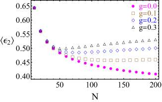
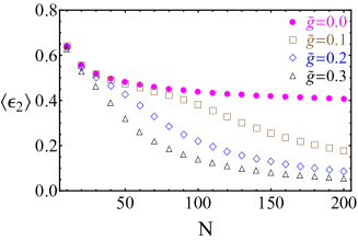
Figure 15: Attractive interaction: $g=0.1,0.2,0.3$ ($\mathbb{Left}$).    Repulsive interaction: $\tilde{g}=0.1,0.2,0.3$ ($\mathbb{Right}$).

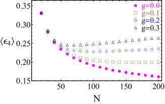
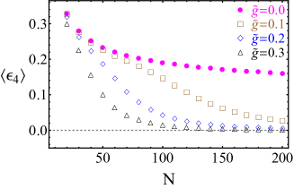
Figure 16: Attractive interaction: $g=0.1,0.2,0.3$ ($\mathbb{Left}$).    Repulsive interaction: $\tilde{g}=0.1,0.2,0.3$ ($\mathbb{Right}$).

For general $b$, the numerical results of $\left<\epsilon_{2}\right>$ and $\left<\epsilon_{4}\right>$ are displayed in Fig. 15 and Fig. 16 respectively.

To show the transverse cross correlations it is also useful to use the cross moments Bzdak et al. (2014); Kalaydzhyan and Shuryak (2014)

$$\left(\epsilon_{n}\{2\}\right)^{2} = \left<\left|\epsilon_{n}\right|^{2}\right>$$

$$\left(\epsilon_{n}\{4\}\right)^{4} = -\left<\left|\epsilon_{n}\right|^{4}\right>+2\left<\left|\epsilon_{n}\right|^{2}\right>^{2}$$

$$\left(\epsilon_{n}\{6\}\right)^{6} = \frac{1}{4}\left[\left<\left|\epsilon_{n}\right|^{6}\right>-9\left<\left|\epsilon_{n}\right|^{4}\right>\left<\left|\epsilon_{n}\right|^{2}\right>+12\left<\left|\epsilon_{n}\right|^{2}\right>^{3}\right]$$

$$\left(\epsilon_{n}\{8\}\right)^{8} = \frac{1}{33}\left[-\left<\left|\epsilon_{n}\right|^{8}\right>+16\left<\left|\epsilon_{n}\right|^{6}\right>\left<\left|\epsilon_{n}\right|^{2}\right>+18\left<\left|\epsilon_{n}\right|^{4}\right>^{2}-144\left<\left|\epsilon_{n}\right|^{4}\right>\left<\left|\epsilon_{n}\right|^{2}\right>^{2}+144\left<\left|\epsilon_{n}\right|^{2}\right>^{4}\right]$$ (7.0.19)

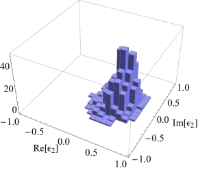
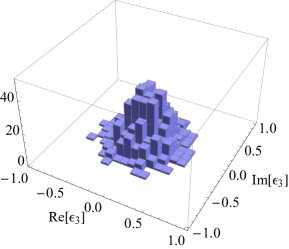
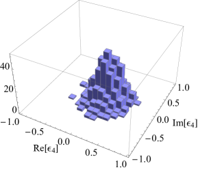
Figure 17: 3D Histograms, 1000 random generated strings. N=200.

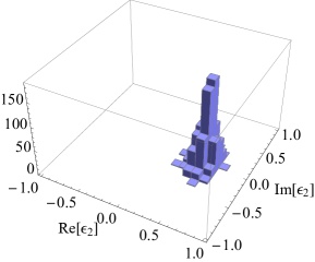
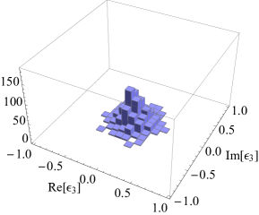
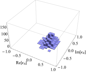
Figure 18: 3D Histograms, 1000 random generated strings. N=200. Attractive interaction $g=0.3$.

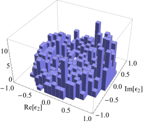
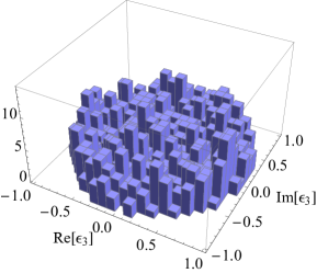
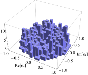
Figure 19: 3D Histograms, 1000 random generated strings. N=200. Repulsive interaction $\tilde{g}=0.3$.

To characterize the initial azimuthal deformation of the string bits in the transverse collision plane, we show in Fig. 17 the pdf distributions of 1000 randomly generated strings at a resolution of $N=200$ with no self-interactions $g/\tilde{g}=0$. The pdf shown are for the distributions in $\epsilon_{2,3,4}$ respectively. We also show in Fig. 18 the pdf distributions of 1000 randomly generated strings at a resolution of $N=200$ undergoing string bit attractions with $g=0.3$ in the mean-field approximation. Note the strong dipole deformation in the leftmost figure. The same pdf for the repulsive case with $\tilde{g}=0.3$ are shown in Fig. 19. The linear spreading of the string bits with the resolution $N$ causes the azimuthal deformations to be relatively uniform.

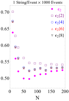
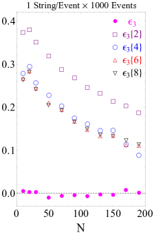
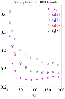
Figure 20: Attractive interaction $g=0.3$.

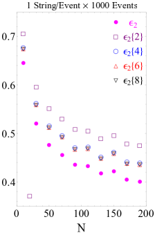
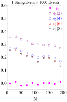
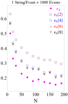
Figure 21: Non-interacting $g/\tilde{g}=0$.

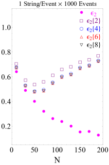
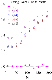
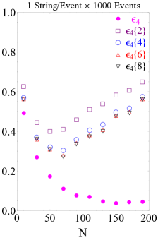
Figure 22: Repulsive interaction $\tilde{g}=0.3$.

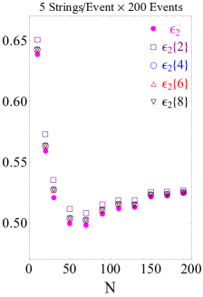
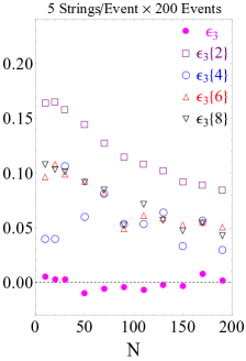
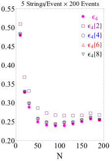
Figure 23: Attractive interaction $g=0.3$.

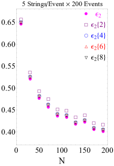
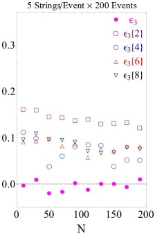
Figure 24: Non-interacting $g/\tilde{g}=0$.

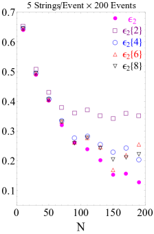
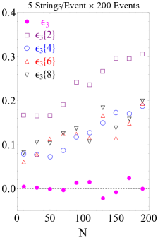
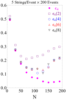
Figure 25: Repulsive interaction $\tilde{g}=0.3$.

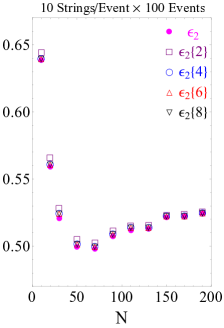
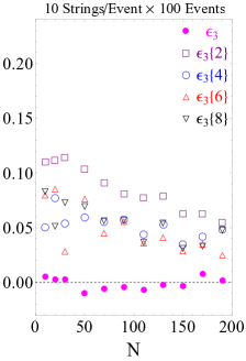
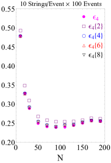
Figure 26: Attractive interaction $g=0.3$.

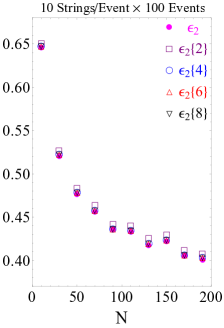
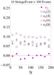
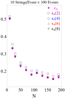
Figure 27: Non-interacting $g/\tilde{g}=0$.

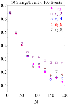
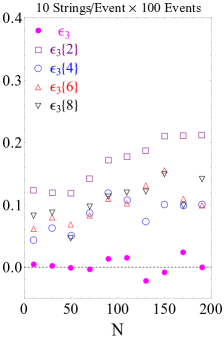
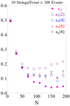
Figure 28: Repulsive interaction $\tilde{g}=0.3$.

For completeness we show the behavior of the cross moments with the resolution for attractive, non-interacting and repulsive strings in Fig. 20, Fig. 21 and Fig. 22 respectively by sampling 1000 times a single string streched with $b=5$. The attraction is set at $g=0.3$ while the repulsion at $\tilde{g}=0.3$ for the infinite range case with $m=0$. Recall that the realistic case of a massive glueball or scalar mass $m$ is amenable to $m=0$ by appropriately decreasing $g$ or $\tilde{g}$. In a typical $pp$ collision at collider energies, we expect to exchange about 10 such long strings Stoffers and Zahed (2013a); Stoffers and Zahed (2012); Stoffers and Zahed (2013b). In Fig. 23, Fig. 24 and Fig. 25 we show the same cross moments following from the exchange of 5 typical strings streched at $b=5$ sampled 200 times for the attractive, non-interacting and repulsive case respectively. The case where 10 string are exchanged is shown in Fig. 26, Fig. 27 and Fig. 28 for the same arrangements of parameters with each 10 string event sampled 100 times. The critical moments for the pre-saturation coupling $g\approx 1/\sqrt{N}\approx 0.01$ are not much different from the $g=0$ presented here. We note that $\epsilon_{n}\{4\}\approx\epsilon_{n}\{6\}\approx\epsilon_{n}\{8\}$ in agreement with suggestion made in Bzdak et al. (2014). The more string exchanges, the denser and more symmetric the transverse string bit distribution for a fixed resolution $N$, the smaller the cross moments. Fig. 27 should represent typical cross moments in $pp$ collisions at collider energies such as RHIC and LHC for minimum bias events. For the high multiplicity $pp$ and $pA$ events reported at LHC hot string configurations near the Hagedorn temperature are needed. They will be discussed in a sequel.

VIII Conclusions

Long holographic strings in walled AdS₅ and $D_{\perp}=3$ provides for a dual description of diffractive scattering and production as well as low-x DIS Stoffers and Zahed (2013a). Although a key aspect of AdS₅ is its conformality which translates to the conformal character of QCD in the UV, the essentials of the walled AdS₅ construction for the holographic string with a large rapidity interval can be captured by a relatively cold transverse string with an effective transverse dimension $2<D_{\perp}<3$. The Pomeron intercept follows from the zero point motion or Luscher term of the free transverse string with $D_{\perp}/12$, and the Pomeron slope is fixed by the string tension.

At low-x, DIS scattering of a small dipole of size $1/Q$ scattering off a fixed target dipole can be regarded as the exchange of a streched string with fixed parameter $b$ with a large rapidity interval ${\rm ln}(1/x)$. Although the DIS structure function averages over all impact parameters, the dominant contribution to this averaging stems from relatively large $b/l_{s}\gg 1$ in units of the string scale $l_{s}\approx 0.1$ fm. Therefore low-x studies could be turned to the studies of a transverse holographic string at higher and higher resolution, a dual description to the wee parton description in perturbative QCD. An essential aspect of the partonic description is Gribov transverse diffusion which arises naturally in the quantum string description as emphasized by Susskind and others Susskind and Griffin (1994); Susskind (1995); Damour and Veneziano (2000); Horowitz and Polchinski (1997).

The wee parton description at low-x can be mapped on a discretized transverse string in $N=1/x$ string bits Susskind and Griffin (1994); Karliner et al. (1988). We have shown that the quantum description of a free transverse and discretized string in $D_{\perp}=3$ results in highly deformed geometries for the string sizes and shapes when the string is streched at fixed impact parameter. We have suggested that at high resolution or string bits, string self-interactions can be captured by a mean-field pair interaction between the string bits. The pair interaction is characterized by a coupling $g$ and a range $1/m$ both of which are inter-changeble by re-scaling. The holographic origin of the transverse string allows for the identification of $g$ with the bulk Newtonian-like constant for $m=0$. As a result a Planck scale emerges for holographic strings at high resolution in $D_{\perp}=3$. In terms of the gauge coupling $\alpha_{s}$, the holographic Planck scale is identified as $l_{P}\approx\alpha_{s}^{2/3}l_{s}$.

In flat dimensions and for relatively weak self-interactions, we have found that the string initial diffusive growth undergoes a first order change into a smaller and fixed size transverse string of the order of few string lengths at a resolution of $x_{c}\approx 0.001$ and for a small string coupling $g_{s}\approx 0.1$. We have identified this change with a pre-saturation stage whereby the string geometry is fixed and small, but the transverse string bit density is still dilute on the Planck scale $l_{p}^{3}n_{\perp}\approx 0.01$. At a much higher resolution or $x_{s}\approx 10^{-5}$ we have found that the transverse string bit density saturates the Bekenstein bound of one bit per Planck scale. We have identified this point with the saturation scale.

In curved dimensions, a simple estimate can be made by noting that the curvature causes the string interaction to take place effectively in lower dimension with $D_{\perp}\rightarrow D_{\perp}(\lambda)$. A similar observation was made in Stoffers and Zahed (2013a); Stoffers and Zahed (2012); Stoffers and Zahed (2013b) for the Pomeron intercept. The result is a smoothening of the transition to the Bekenstein bound observed in flat $D_{\perp}=3$. Saturation was found to take place at a higher value of small-x or $x_{s}\approx 10^{-3}$.

The geometry of the string bit distributions emerging from streched strings for a typical impact parameter of $b=5\equiv 10\,l_{s}$ is rich in structure and transverse deformation. We have presented a detailed study of its transverse moments and moment distributions for single and multiple string exchanges. These prompt and deformed distributions can be used to initialize the prompt parton distributions in current $pp$ and $pA$ collisions in colliders at high resolution or low-x. The large deformations observed in this analysis show that they can yield large transverse asymmetries in prompt multi-particle production in the Pomeron kinematics. Also they may translate to large transverse momentum asymmetries in the flow analyses of multiplicity at current collider energies. We plan to address some of these issues next.

IX Acknowledgements

We thank Dima Kharzeev and Edward Shuryak for discussions. This work was supported by the U.S. Department of Energy under Contract No. DE-FG-88ER40388.

X Appendix

In this Appendix we discuss a simple phenomenological way of introducing the effects of AdS₅ warping on the transverse oscillators in (2.0.1) that reproduces the key property of Gribov diffusion derived in Stoffers and Zahed (2013a); Stoffers and Zahed (2012); Stoffers and Zahed (2013b). For that we introduce the rescalings $\tau\rightarrow\lambda_{\tau}\tau$ and $b\rightarrow\tilde{b}$, so that (2.0.1) now reads

$$S_{\perp}=\frac{\sigma_{T}}{2}\int d\tau\int_{0}^{\pi}d\sigma\ \ \left[\frac{1}{\lambda_{\tau}^{2}}\left(\dot{x}_{\perp}\right)^{2}+\left({x^{\prime}}_{\perp}\right)^{2}\right]$$ (10.0.1)

with the end-point condition

$$x_{\perp}^{i}(\sigma=0,\tau)=0\ \ \ \ \ \ x_{\perp}^{i}(\sigma=\pi,\tau)=\mathbb{\tilde{b}}^{i}$$ (10.0.2)

The Lagrangian for the discretized string is now

$$\mathcal{L}_{\perp}=\frac{1}{\lambda_{\tau}^{2}}\frac{1}{N}\sum_{k=0}^{N}\left(\dot{x}_{\perp}^{i}(k)\right)^{2}-\frac{1}{N}\sum_{k=1}^{N}\left(\frac{x_{\perp}^{i}(k)-x_{\perp}^{i}(k-1)}{\frac{\pi}{N}}\right)^{2}$$ (10.0.3)

The mode decompostion for the amplitudes $x_{\perp}^{i}$ reads

$$x_{\perp}^{i}(k,\tau)=\lambda_{\tau}\mathbb{\tilde{b}}^{i}\frac{k}{N}+\lambda_{\tau}\sum_{n=1}^{N-1}X_{n}^{i}(\tau)\sin\left(\frac{nk}{N}\pi\right)\ \ \ \ \ \ \ \ \ (k=0,1,\cdots,N)$$ (10.0.4)

and their conjugate momenta are

$$p_{\perp}^{i}(k,\tau)=\frac{\partial\mathcal{L}}{\partial\dot{x}_{\perp}^{i}}=\frac{1}{\lambda_{\tau}^{2}}\frac{2}{N}\dot{x}_{\perp}^{i}=\frac{1}{\lambda_{\tau}}\frac{2}{N}\sum_{n=1}^{N-1}\dot{X}_{n}^{i}(\tau)\sin\left(\frac{nk}{N}\pi\right)\equiv\frac{1}{\lambda_{\tau}}\frac{2}{N}\sum_{n=1}^{N-1}P_{n}^{i}(\tau)\sin\left(\frac{nk}{N}\pi\right)$$ (10.0.5)

Thus, the Hamiltonian

$$\mathcal{H}_{\perp}=\frac{1}{2}\sum_{n=1}^{N-1}\left(P_{n}^{i}(\tau)P_{n}^{i}(\tau)+\lambda_{\tau}^{2}\Omega_{n}^{2}{X}_{n}^{i}(\tau){X}_{n}^{i}(\tau)\right)+\lambda_{\tau}^{2}\frac{\tilde{b}^{2}}{\pi^{2}}$$ (10.0.6)

The ground state of this dangling N-string is a product of warped Gaussians

$$\Psi[\lambda_{\tau};X]=\prod_{n,i}\Psi(\lambda_{\tau};X_{n}^{i})=\prod_{n,i}\left(\frac{\lambda_{\tau}\Omega_{n}}{\pi}\right)^{\frac{1}{4}}\exp\left[-\frac{\lambda_{\tau}\Omega_{n}}{2}(X_{n}^{i})^{2}\right]$$ (10.0.7)

leading to the ground state energy

$$\left<\mathcal{H}_{\perp}\right>=\frac{D_{\perp}\lambda_{\tau}}{2}\sum_{n=1}^{N-1}\Omega_{n}+\frac{\lambda_{\tau}^{2}\tilde{b}^{2}}{\pi^{2}}$$ (10.0.8)

(2.0.9) is recovered for $\lambda_{\tau}=1$ as it should. If we set $\lambda_{\tau}={D_{\perp}(\lambda)}/{D_{\perp}}$ and $\tilde{b}={b}/{\lambda_{\tau}}$, (10.0.8) reads as

$$\left<\mathcal{H}_{\perp}\right>=\frac{D_{\perp}(\lambda)}{2}\sum_{n=1}^{N-1}\Omega_{n}+\frac{b^{2}}{\pi^{2}}$$ (10.0.9)

The string transverse squared size (II) is now

$$R_{\perp}^{2}=\frac{1}{N}\sum_{k=0}^{N}\left<\left(x_{k}^{i}-\mathbb{b}^{i}\frac{k}{N}\right)^{2}\right>=\lambda_{\tau}^{2}\frac{D_{\perp}}{4}\sum_{n=1}^{N-1}\frac{1}{\lambda_{\tau}\Omega_{n}}=\frac{D_{\perp}(\lambda)}{4}\sum_{n=1}^{N-1}\frac{1}{\Omega_{n}}\approx\frac{D_{\perp}(\lambda)}{4}\,{\rm ln}(N)$$ (10.0.10)

with a Pomeron intercept $D_{\perp}(\lambda)/12$.

Figure 14: Saturation (red), pre-saturation (blue) and diffusive (green) regimes for a transverse string with decreasing resolution in $D_{\perp}(\lambda)$. See text.

References

- Donnachie and Landshoff (1992) A. Donnachie and P. Landshoff, Phys.Lett. B296, 227 (1992), eprint hep-ph/9209205.
- Gribov and Lipatov (1972) V. Gribov and L. Lipatov, Sov.J.Nucl.Phys. 15, 438 (1972).
- Gribov (2003) V. N. Gribov, The Theory of Complex Angular Momenta (Cambridge University Press, 2003), ISBN 9780511534959, cambridge Books Online, URL http://dx.doi.org/10.1017/CBO9780511534959.
- Kuraev et al. (1976) E. A. Kuraev, L. N. Lipatov, and V. S. Fadin, Sov.Phys.JETP 44, 443 (1976).
- Lipatov (1976) L. Lipatov, Sov.J.Nucl.Phys. 23, 338 (1976).
- Sterman (1999) G. F. Sterman (1999), eprint hep-ph/9905548.
- Fadin et al. (1975) V. S. Fadin, E. Kuraev, and L. Lipatov, Phys.Lett. B60, 50 (1975).
- Balitsky and Lipatov (1978) I. Balitsky and L. Lipatov, Sov.J.Nucl.Phys. 28, 822 (1978).
- Veneziano (1968) G. Veneziano, Nuovo Cim. A57, 190 (1968).
- Greensite (1985) J. Greensite, Nucl.Phys. B249, 263 (1985).
- Maldacena (1998) J. M. Maldacena, Phys.Rev.Lett. 80, 4859 (1998), eprint hep-th/9803002.
- Rho et al. (1999) M. Rho, S.-J. Sin, and I. Zahed, Phys.Lett. B466, 199 (1999), eprint hep-th/9907126.
- Janik and Peschanski (2000) R. Janik and R. B. Peschanski, Nucl.Phys. B586, 163 (2000), eprint hep-th/0003059.
- Janik (2001) R. A. Janik, Phys.Lett. B500, 118 (2001), eprint hep-th/0010069.
- Polchinski and Strassler (2002) J. Polchinski and M. J. Strassler, Phys.Rev.Lett. 88, 031601 (2002), eprint hep-th/0109174.
- Polchinski and Susskind (2001) J. Polchinski and L. Susskind, pp. 105–114 (2001), eprint hep-th/0112204.
- Polchinski and Strassler (2003) J. Polchinski and M. J. Strassler, JHEP 0305, 012 (2003), eprint hep-th/0209211.
- Brower et al. (2007) R. C. Brower, J. Polchinski, M. J. Strassler, and C.-I. Tan, JHEP 0712, 005 (2007), eprint hep-th/0603115.
- Brower et al. (2009) R. C. Brower, M. J. Strassler, and C.-I. Tan, JHEP 0903, 092 (2009), eprint 0710.4378.
- Brower et al. (2010) R. C. Brower, M. Djuric, I. Sarcevic, and C.-I. Tan, JHEP 1011, 051 (2010), eprint 1007.2259.
- Brower et al. (2011) R. C. Brower, M. Djuric, I. Sarcevic, and C.-I. Tan (2011), eprint 1106.5681.
- Hatta et al. (2008a) Y. Hatta, E. Iancu, and A. Mueller, JHEP 0801, 063 (2008a), eprint 0710.5297.
- Hatta et al. (2008b) Y. Hatta, E. Iancu, and A. Mueller, JHEP 0801, 026 (2008b), eprint 0710.2148.
- Albacete et al. (2008) J. L. Albacete, Y. V. Kovchegov, and A. Taliotis, JHEP 0807, 074 (2008), eprint 0806.1484.
- Albacete et al. (2009) J. L. Albacete, Y. V. Kovchegov, and A. Taliotis, AIP Conf.Proc. 1105, 356 (2009), eprint 0811.0818.
- Basar et al. (2012) G. Basar, D. E. Kharzeev, H.-U. Yee, and I. Zahed, Phys.Rev. D85, 105005 (2012), eprint 1202.0831.
- Stoffers and Zahed (2013a) A. Stoffers and I. Zahed, Phys.Rev. D87, 075023 (2013a), eprint 1205.3223.
- Stoffers and Zahed (2012) A. Stoffers and I. Zahed (2012), eprint 1210.3724.
- Stoffers and Zahed (2013b) A. Stoffers and I. Zahed, Acta Phys.Polon.Supp. 6, 7 (2013b).
- Qian and Zahed (2012) Y. Qian and I. Zahed (2012), eprint 1211.6421.
- Shuryak and Zahed (2014) E. Shuryak and I. Zahed, Phys.Rev. D89, 094001 (2014), eprint 1311.0836.
- Bergman and Thorn (1997) O. Bergman and C. B. Thorn, Nucl.Phys. B502, 309 (1997), eprint hep-th/9702068.
- Karliner et al. (1988) M. Karliner, I. R. Klebanov, and L. Susskind, Int.J.Mod.Phys. A3, 1981 (1988).
- Susskind and Griffin (1994) L. Susskind and P. Griffin (1994), eprint hep-ph/9410306.
- Susskind (1995) L. Susskind, J.Math.Phys. 36, 6377 (1995), eprint hep-th/9409089.
- Froissart (1961) M. Froissart, Phys.Rev. 123, 1053 (1961).
- Bekenstein (1973) J. D. Bekenstein, Phys.Rev. D7, 2333 (1973).
- Bekenstein (1972) J. Bekenstein, Lett.Nuovo Cim. 4, 737 (1972).
- Bekenstein (1974) J. D. Bekenstein, Phys.Rev. D9, 3292 (1974).
- Hawking (1974) S. Hawking, Nature 248, 30 (1974).
- Hawking (1975) S. Hawking, Commun.Math.Phys. 43, 199 (1975).
- Cornalba et al. (2010a) L. Cornalba, M. S. Costa, and J. Penedones, Phys.Rev.Lett. 105, 072003 (2010a), eprint 1001.1157.
- Cornalba et al. (2010b) L. Cornalba, M. S. Costa, and J. Penedones, JHEP 1003, 133 (2010b), eprint 0911.0043.
- Cornalba and Costa (2008) L. Cornalba and M. S. Costa, Phys.Rev. D78, 096010 (2008), eprint 0804.1562.
- McLerran (2002) L. D. McLerran, Lect.Notes Phys. 583, 291 (2002), eprint hep-ph/0104285.
- Tapia Takaki (2010) J. Tapia Takaki (ALICE), J.Phys. G37, 094050 (2010).
- Iancu and Venugopalan (2003) E. Iancu and R. Venugopalan (2003), eprint hep-ph/0303204.
- Iancu et al. (2002) E. Iancu, A. Leonidov, and L. McLerran, pp. 73–145 (2002), eprint hep-ph/0202270.
- Navelet and Peschanski (2002) H. Navelet and R. B. Peschanski, Nucl.Phys. B634, 291 (2002), eprint hep-ph/0201285.
- Iancu (2001) E. Iancu, pp. 184–191 (2001), eprint hep-ph/0111400.
- Levin (2001) E. Levin (2001), eprint hep-ph/0105205.
- McLerran and Venugopalan (1994) L. D. McLerran and R. Venugopalan, Phys.Rev. D49, 3352 (1994), eprint hep-ph/9311205.
- Gelis et al. (2010) F. Gelis, E. Iancu, J. Jalilian-Marian, and R. Venugopalan, Ann.Rev.Nucl.Part.Sci. 60, 463 (2010), eprint 1002.0333.
- Marquet et al. (2005) C. Marquet, A. Mueller, A. Shoshi, and S. Wong, Nucl.Phys. A762, 252 (2005), eprint hep-ph/0505229.
- Iancu and Mueller (2004) E. Iancu and A. Mueller, Nucl.Phys. A730, 460 (2004), eprint hep-ph/0308315.
- Iancu (2009) E. Iancu, Nucl.Phys.Proc.Suppl. 191, 281 (2009), eprint 0901.0986.
- Gelis (2013) F. Gelis, Int.J.Mod.Phys. A28, 1330001 (2013), eprint 1211.3327.
- Tribedy and Venugopalan (2012) P. Tribedy and R. Venugopalan, Phys.Lett. B710, 125 (2012), eprint 1112.2445.
- Tribedy and Venugopalan (2011a) P. Tribedy and R. Venugopalan (2011a), eprint 1101.5922.
- Tribedy and Venugopalan (2011b) P. Tribedy and R. Venugopalan, Nucl.Phys. A850, 136 (2011b), eprint 1011.1895.
- Qian and Zahed (2014) Y. Qian and I. Zahed (2014), eprint 1410.1092.
- Kalaydzhyan and Shuryak (2014) T. Kalaydzhyan and E. Shuryak, Phys.Rev. D90, 025031 (2014), eprint 1402.7363.
- Liu and Zahed (2014a) Y. Liu and I. Zahed (2014a), eprint 1408.3331.
- Liu and Zahed (2014b) Y. Liu and I. Zahed (2014b), eprint 1407.0384.
- Damour and Veneziano (2000) T. Damour and G. Veneziano, Nucl.Phys. B568, 93 (2000), eprint hep-th/9907030.
- Golec-Biernat and Wusthoff (1998) K. J. Golec-Biernat and M. Wusthoff, Phys.Rev. D59, 014017 (1998), eprint hep-ph/9807513.
- Golec-Biernat and Wusthoff (1999) K. J. Golec-Biernat and M. Wusthoff, Phys.Rev. D60, 114023 (1999), eprint hep-ph/9903358.
- Rezaeian et al. (2013) A. H. Rezaeian, M. Siddikov, M. Van de Klundert, and R. Venugopalan, Phys.Rev. D87, 034002 (2013), eprint 1212.2974.
- Kowalski and Teaney (2003) H. Kowalski and D. Teaney, Phys.Rev. D68, 114005 (2003), eprint hep-ph/0304189.
- Bzdak et al. (2014) A. Bzdak, P. Bozek, and L. McLerran, Nucl.Phys. A927, 15 (2014), eprint 1311.7325.
- Horowitz and Polchinski (1997) G. T. Horowitz and J. Polchinski, Phys.Rev. D55, 6189 (1997), eprint hep-th/9612146.