Uncertainty Quantification for Airfoil Icing using Polynomial Chaos Expansions

Abstract

The formation and accretion of ice on the leading edge of a wing can be detrimental to airplane performance. Complicating this reality is the fact that even a small amount of uncertainty in the shape of the accreted ice may result in a large amount of uncertainty in aerodynamic performance metrics (e.g., stall angle of attack). The main focus of this work concerns using the techniques of Polynomial Chaos Expansions (PCE) to quantify icing uncertainty much more quickly than traditional methods (e.g., Monte Carlo). First, we present a brief survey of the literature concerning the physics of wing icing, with the intention of giving a certain amount of intuition for the physical process. Next, we give a brief overview of the background theory of PCE. Finally, we compare the results of Monte Carlo simulations to PCE-based uncertainty quantification for several different airfoil icing scenarios. The results are in good agreement and confirm that PCE methods are much more efficient for the canonical airfoil icing uncertainty quantification problem than Monte Carlo methods.

Nomenclature

$u$	State vector
$x,t,Z$	Physical space vector, time, and stochastic parameter vector
$y$	Observable vector
$\rho(Z)$	Probability density function (PDF) of $Z$
$\Gamma$	Support of Z
$\phi(Z)$	Univariate polynomial chaos basis function of $Z$
$\Phi(Z)$	Multivariate polynomial chaos basis function of $Z$
$h_{i}$	Norm of the $i^{th}$ polynomial chaos basis function
$\mathbb{P}_{N}$	$N^{th}$-order projection operator
$R,S_{r}$	Radius and chordwise-position (aft of leading edge) of the ridge ice shape
$dR,dS_{r}$	Perturbations in the ridge ice parameters $R$ and $S_{r}$ from the mean ridge ice shape
$H,S_{h}$	Height (normal to airfoil surface) and separation distance of the horn ice shape
$h,s$	Scaling parameters for the height $H$ and separation distance $S_{h}$ of the horn ice shape
$\mu,\sigma$	Mean and standard deviation
${C_{L}}_{\text{max}}$	Maximum lift coefficient in the steady flowfield regime
$\alpha_{\text{max}}$	Angle of attack at ${C_{L}}_{\text{max}}$
$L/D_{MAX}$	Maximum lift to drag ratio
$c$	Chord length

1 Introduction

Wing icing can present a significant safety hazard to pilots. Wing ice shapes are often sharp and jagged in profile and rough in surface texture; both of these characteristics tend to induce flow separation at angles of attack which are often quite mild. This can cause stall at lower angles of attack than those to which pilots are accustomed. It is for this reason that wing icing has been identified as the cause of 388 crashes between 1990 and 2000 [1].

Equally troubling is the fact that wing icing is a process which is associated with a high degree of uncertainty in practice. The reasons for this are fairly intuitive: icing itself is fundamentally a complex physics problem, in which both aerodynamics and thermodynamics are involved and highly coupled. Additionally, wing icing codes such as NASA’s LEWICE often make “rule of thumb” approximations and educated guesses at the physical parameters governing the process[2, 3]. Lastly, it is obvious that, in flight, pilots can never know all of the many physical parameters which contribute to the icing process with perfect certainty, since there is always some uncertainty in weather-related information such as the liquid water content of the free-stream air, the ambient temperature, the temperature of the wing surface, etc.

The main focus of this work is to describe a fast, accurate framework for quantifying the uncertainty which arises in aerodynamic performance metrics (e.g., stall angle of attack, max lift coefficient, etc.) as a direct result of uncertainty in a set of parameters which govern the airfoil ice shape.

2 Wing Icing: Background

The consensus in the literature is that wing icing may be conveniently divided into a few simple classifications. Each of these is briefly discussed in turn. The interested reader is referred to the literature for a more in-depth discussion[4].

2.1 Streamwise Ice

As the name implies, this scenario is characterized by relatively low amounts of smooth ice accumulation which closely follow the airfoil contour [4]. Aerodynamically, therefore, this ice is much less detrimental to performance than the other classifications. Hence, we do not pursue it in this work any further.

2.2 Ice Roughness

This situation is characterized by the development of a region of smooth ice near the stagnation point which transitions aft to rough ice and then to several small, sharp, jagged ice “feathers.” [4] Depending on the size of the feathers relative to the scale of the boundary layer, the feathers can act as flow obstacles and promote separation. Aerodynamically, the distinction between this scenario and the more familiar ice horn is not always clear (with the exception that ice horns are primarily a two-dimensional (2D) phenomenon, while the ice feathers may exhibit three-dimensional (3D) effects).While ice roughness may lead to early trailing-edge separation, it typically does not cause the large scale separation bubbles which the more malignant horn and ridge ice do. For these reasons, we will not discuss this situation any further in this work.

2.3 Ridge Ice

In this scenario, a ridge forms aft of the stagnation point, as illustrated in Figure 1(a). This situation is particularly dangerous for two reasons. First, the ridge formation is jagged and discontinuous, which promotes large scale separation at relatively low angles of attack. Second, the ridge accumulates just aft of the deicing equipment, and hence it is not possible to combat this type of ice with traditional deicing mechanisms. The ridge profile is typically modeled as either a forward or backward facing quarter circle round. It is predominantly a 2D phenomenon, and the major parameters which describe the profile shape are the radius of the quarter circle round and its position aft of the leading edge [4, 5].

2.4 Horn Ice

Horn ice forms in icing conditions which are relatively warmer with higher amounts of liquid water content in the free-stream. It can be understood in terms of a division between areas near the stagnation point of the airfoil, for which rates of ice accretion are lower, and areas aft of that, which experience higher rates. Initially (i.e., before the horn has begun to form), this division is due to a coupling between aerodynamics and thermodynamics: the boundary layer near the stagnation point is laminar, while aft of that point it transitions to a turbulent profile, and the local convective heat transfer rate is lower for laminar boundary layers than it is for turbulent ones [6]. As time progresses, however, surface roughness becomes the dominant driving force in the creation of the horn. Near the stagnation point, a thin, uniform film of water develops on the ice surface, which keeps the ice surface smooth. Aft of the stagnation point, the ice surface is mostly dry, with water beadlets intermittently dispersed. When these beadlets freeze, they roughen the ice surface, and convective heat transfer is higher for rougher ice surfaces than for smoother ones. Because convection dominates the heat transfer, it is this division in local convective heat transfer that is thermodynamically responsible for horn ice [7]. Horn ice is primarily 2D. The major parameters used to describe the profile shape in this work are the horn height (normal to the airfoil surface) and separation distance between the horns.

3 Polynomial Chaos

The ultimate goal of this work is the quantification of uncertainty in aerodynamic performance metrics, resulting from uncertainty in the parameters that govern the ice shape (whether ridge or horn). Traditionally, uncertainty quantification (UQ) problems such as this have been approached through Monte Carlo methods. The main drawback of these methods is that they are sampling-based, and as such often require undesirably or unfeasibly large sample sizes. A relatively new alternative to this approach which is gaining increasing popularity is to use polynomial chaos expansions (PCE).

Weiner coined the term “polynomial chaos” when studying the decomposition of Gaussian processes with Hermite polynomials. It was Ghanem and Spanos, however, who first introduced the stochastic spectral method for systems with Gaussian input processes using the Hermite polynomials as a basis [8]. Xiu and Karniadakis later generalized this spectral approach to account for non-Gaussian input processes by using orthogonal polynomials different from the Hermite basis [9].

There are two main approaches to UQ using PCE: the stochastic Galerkin method, and the stochastic collocation method (see Xiu[9] for more information about both). The first method can be thought of as an extension of traditional Galerkin methods. The governing stochastic equations are orthogonally projected onto the span of a PCE basis, and all expansions are truncated at finite order. This results in a new system of coupled, deterministic equations which must be solved for the modes of the solution expansion. The stochastic collocation method, on the other hand, is essentially a discrete Galerkin approach, whereby the integrals in the projection equations are approximated by a quadrature rule of sufficient accuracy. This process results in the evaluation of the governing equation at a finite number of nodes, or “collocation points.”

There are advantages and disadvantages to either of these approaches. The stochastic Galerkin approach can be very difficult to implement when the governing equations are large or complicated, since the new, coupled equations must be first derived and then solved. The stochastic collocation method, on the other hand, does not require the derivation of new equations, and so any legacy codes for solving the original equations may still be used. It should be noted, however, that the stochastic collocation method can suffer from aliasing error if the quadrature mesh is too coarse; the stochastic Galerkin method does not suffer from this.

In this work, we use the stochastic collocation method for UQ. We give a brief overview of this approach below; further details can be found in introductory references on PCE methods[8, 9].

3.1 Stochastic Collocation Method

Let $Z=(Z_{1},Z_{2})$ be a vector of random variables that parameterize the uncertain quantities in the ice shape. For instance, for ridge ice, these parameters will be the location and height of the ridge, and for horn ice, these will specify the horn height and separation distance. We are interested in the corresponding uncertainty of an aerodynamic quantity, represented by $y(Z)$. For instance, $y(Z)$ could be the maximum lift coefficient, angle of attack at which the maximum lift occurs, or maximum $L/D$.

In our setting, the true values of $y(Z)$ are determined by a 2D steady-state RANS calculation. A particular value of $Z$ specifices the boundary conditions, and we solve the RANS equations for these boundary conditions, to determine the resulting aerodynamic quantities.

The goal of the method is to represent $y(Z)$ in terms of some basis functions $\Phi_{i}$, writing

$$y(Z)=\sum_{|i|=0}^{N}y_{i}\Phi_{i}(Z).$$ (1)

Here, $i=(i_{1},i_{2})$ is a multi-index, and $|i|=i_{1}+i_{2}$. We define an inner product on the space of functions of the random variables by

$$\left\langle f,g\right\rangle=\int_{\Gamma}f(Z)g(Z)\rho(Z)\,dZ,$$ (2)

where $\rho(Z)$ denotes the probability density function of $Z$, and has support $\Gamma$. We assume our basis functions are orthonormal with respect to this inner product, so that

$$\left\langle\Phi_{i},\Phi_{j}\right\rangle=\delta_{ij},$$ (3)

where $\delta_{ij}=1$ if $i=j$, and $0$ if $i\neq j$. The coefficients $y_{i}$ in the expansion (1) may then be deterimined by taking an inner product with $\Phi_{j}$: because the $\Phi_{j}$ are orthonormal, we have

$$y_{j}=\left\langle y,\Phi_{j}\right\rangle.$$ (4)

Note that one could also take $y(Z)$ to be a vector of several different aerodynamic quantities of interest: in this case, the coefficients $y_{i}$ in the expansion (1) are vectors, and each component of $y_{i}$ is determined by an equation such as (4), for the corresponding component of $y$.

In the stochastic collocation method, we approximate the inner product in (4) by employing a quadrature rule. In particular, the basis functions $\Phi_{i}$ are chosen to be

$$\Phi_{i}(Z)=\phi_{i_{1}}(Z_{1})\phi_{i_{2}}(Z_{2}),$$ (5)

where $\phi_{n}$ is a (univariate) polynomial of degree $n$. In practice, the $\{\phi_{n}\}$ will be a basis of orthogonal polynomials, chosen so that the orthogonality condition (3) is satisfied. (For instance, if $\rho(Z)$ is a Gaussian distribution, then suitably normalized Hermite polynomials satisfy the orthogonality relation.) To evaluate the inner product, we then choose quadrature nodes $Z^{(k)}$, for $k=1,\ldots,Q$, with corresponding quadrature weights $w_{k}$, and approximate the inner product as

$$y_{j}=\left\langle y,\Phi_{j}\right\rangle\approx\sum_{k=1}^{Q}y(Z^{(k)})\Phi_{j}(Z^{(k)})w_{k}.$$ (6)

In practice, we use a Gauss quadrature rule to deterimine $Z^{(k)}$ and $w_{k}$, taking $N+1$ points for each component of $Z$ (where $N$ is the degree of the polynomial expansion (1)), for a total of $Q=(N+1)^{2}$ nodes and weights. This procedure gives exact results if the integrand is any polynomial of degree $2N+1$ or less in any of the components of $Z$. The resulting model interpolates the true solution between the nodes.

3.2 Statistical Information

If we have a sufficiently accurate PC expansion for the observable, defined as in (1), then we may retrieve statistical moments through a few simple post-processing steps. For example, the mean is approximated by the expected value of the PC expansion: noting that $\Phi_{0}=1$, we have

$$\mu=\mathbb{E}[y]=\int_{\Gamma}y\rho(Z)\,dZ=\left\langle y,\Phi_{0}\right\rangle=y_{0}.$$ (7)

Similarly, the variance can be approximated as

$$\sigma^{2}=\mathbb{E}[(y-\mu)^{2}]=\left\langle y-y_{0},y-y_{0}\right\rangle=\sum_{|i|=1}^{N}y_{i}^{2}.$$ (8)

3.3 Overview of PCE Algorithm for Quantifying Uncertainty

Putting together the results of this section, we can outline a simple set of steps which describes how to implement a PCE-based uncertainty quantification, based on the stochastic collocation method:

1. Choose polynomial chaos basis. The first step is to choose the polynomial chaos basis which is optimal for the chosen application. Here, “optimal” is usually defined in terms of spectral convergence: we wish to select that basis which best represents the input and output probability density functions (PDFs) using the fewest number of modes.

2. Determine collocation points and weights. Here, we wish to determine the mesh of discrete collocation points and weights which are required to evaluate (6). The procedure for selecting the collocation nodes/weights is a straightforward application of Gaussian quadrature techniques.

3. Solve governing equations at collocation points. We obtain the values of $y(Z)$ at each of the collocation points by solving the 2D steady-state RANS equations at each of the collocation points.

4. Obtain the approximate PCE model. This is done by solving (6). Any desired statistical information follows through simple post-processing.

4 Application to Airfoil Icing

The PCE stochastic collocation method presented in the previous section is applied to the ridge and horn ice problems in this section, with the goal of quantifying uncertainty in airfoil aerodynamic performance metrics, such as max lift coefficient and stall angle of attack. The results are compared to Monte Carlo simulations.

We consider two classes of airfoil icing: ridge and horn. Both of these icing cases are modeled as 2D phenomena. The airfoil profile used is the NACA 63A213 at a Reynolds number of $Re=4.5\times 10^{5}$ and Mach number of $M=0.21$; these conditions are chosen in agreement with a those used in a paper which investigated simulated ice accretions using LEWICE [10].

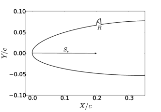
(a) Ridge parameterization.

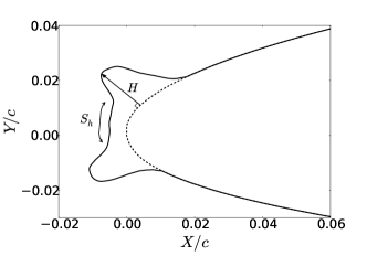
(b) Horn parameterization.

Figure 1: Parameterization convention for the ridge and horn ice scenarios. The figure at the right represents the mean horn ice shape used in this work, obtained from Papadakis[10].

We model ridge ice shapes as backward-facing quarter circle rounds, which are parameterized by the radius $R$ of the round and the location $S_{r}$ aft of the airfoil leading edge (see Fig. 1). The radius $R$ governs uncertainty in the size of the ridge ice, while the position $S_{r}$ governs uncertainty in where the ridge forms aft of the deicing boot.

In all cases, we specify the uncertainty in $R$ and $S_{r}$ as a bivariate Gaussian. In accordance with the literature (see Bragg[4]), we use a mean value for the radius of $\mathbb{E}(R)=1.39\%$ of the chord length, and a mean value for the position of $\mathbb{E}(S_{r})=20\%$ of the chord length.

We select a profile for the mean horn geometry from Papadakis[10]. The two independent stochastic parameters which govern perturbations from the mean shape are the height $H$ (normal to the airfoil surface) and separation distance $S_{h}$ of the horn. The mean horn profile used is shown in Fig. 1.

4.1 Ridge Ice Case

2

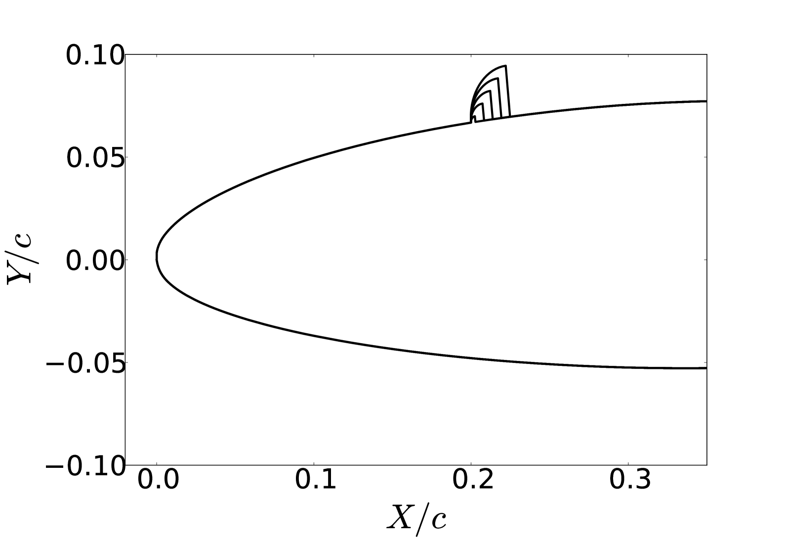
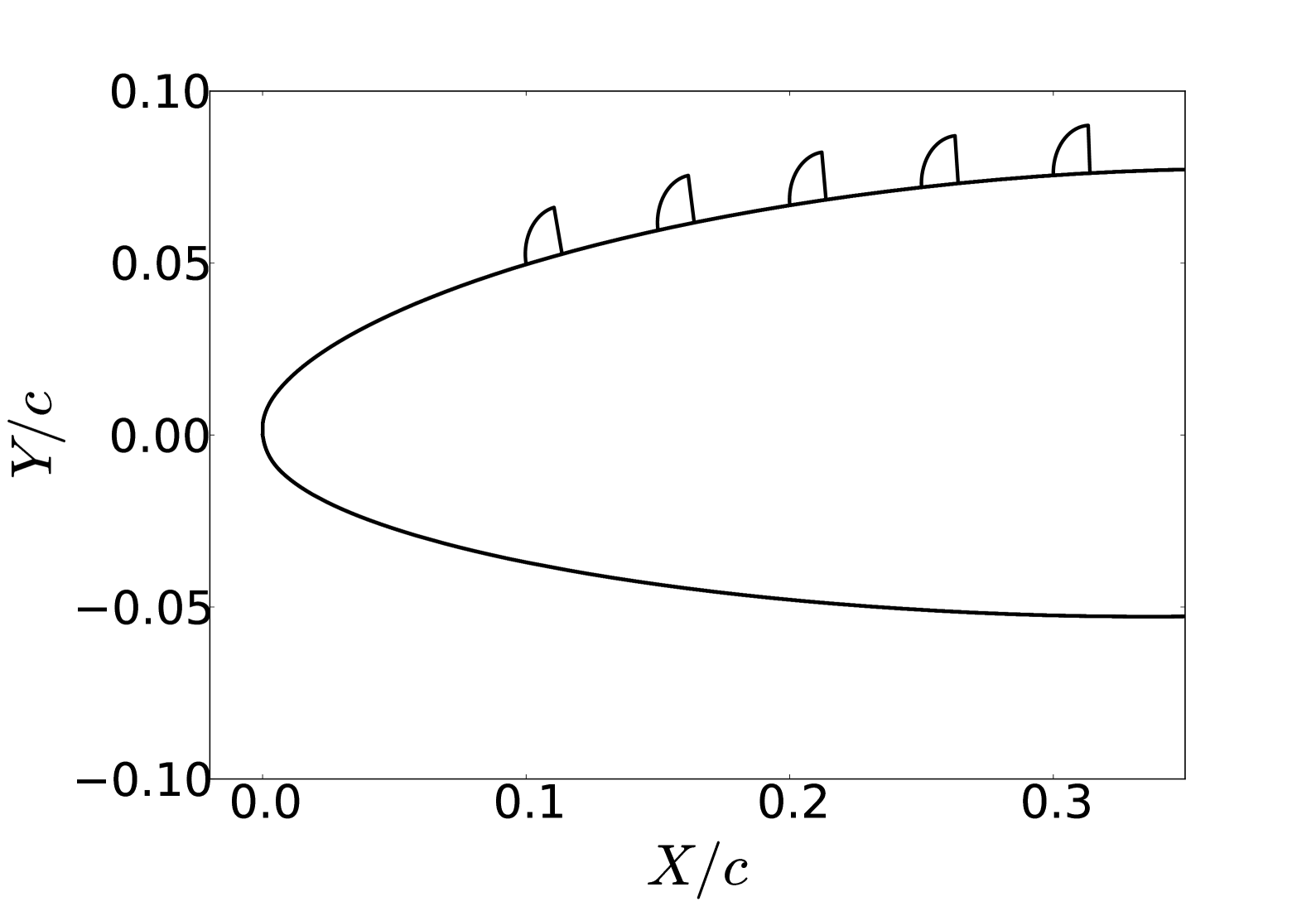
Figure 2: LEFT: Ridge shapes produced by perturbing $R$ by $dR$ = {-2, -1, 0, 1, 2}$\sigma_{R}$ with $\sigma_{R}=40\%$ ($S_{r}=\mu_{S_{r}}$). RIGHT: Ridge shapes produced by perturbing $S_{r}$ by $dS_{r}$ = {-2, -1, 0, 1, 2}$\sigma_{S_{r}}$ with $\sigma_{S_{r}}=5\%$ ($R=\mu_{R}$).

We begin with the ridge ice case, and quantify uncertainty in three separate aerodynamic performace metrics: ${C_{L}}_{\text{max}}$, $\alpha_{\text{max}}$, and $L/D_{\text{max}}$. In each of the cases, there are two uncertain input parameters: ridge radius, $R$, and ridge position, $S_{r}$. Both of these parameters assume independent Gaussian distributions, where $\mu_{R}=1.39\%$ of the chord, and $\mu_{S_{r}}=20\%$ of the chord; these were selected in agreement with Bragg[4]. We specify $\sigma_{R}$ as a percentage of $\mu_{R}$ and $\sigma_{S_{r}}$ as a percentage of the chord length. We present two UQ investigations in which the standard deviation pairs $(\sigma_{R},\sigma_{S_{r}})$ take the values $(10\%,1.25\%)$ and $(40\%,5\%)$.

Note that the flow solver used for all of our ridge and horn geometries is FLO103, a 2D, steady-state Reynolds-Averaged Navier Stokes (RANS) solver developed by Martinelli, Tatsumi, and Jameson [11]. It uses a Spalart-Allmaras turbulence closure model, and uses no-injection, no-slip, adiabatic, isothermal boundary conditions at the wall of the airfoil. Time integration is performed explicitly by multigrid time stepping.

As mentioned, we compare our PCE methods to Quasi Monte Carlo simulations. The basic algorithm used in this scheme involves inverse transform sampling (see Devroye [12]) for selecting samples. The cumulative distribution space is sampled using an ergodic dynamical system. This algorithm has a notable advantage of efficiency over standard Monte Carlo algorithms: it can be proved that the samples obtained through this Quasi Monte Carlo method converge in distribution at a rate proportional to $1/N$, where $N$ is the number of samples [13]. This is in contrast to standard Monte Carlo, in which the rate of convergence is $1/\sqrt{N}$.

3

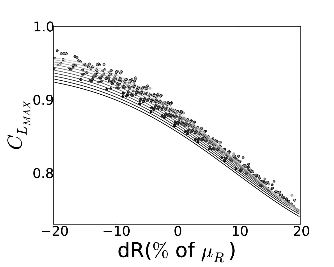
(a) ${C_{L}}_{\text{max}}(dR,dS_{r})$

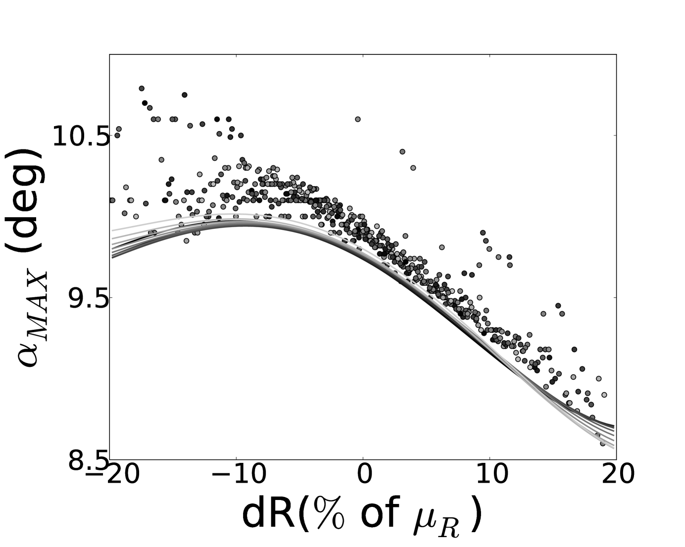
(b) $\alpha_{\text{max}}(dR,dS_{r})$

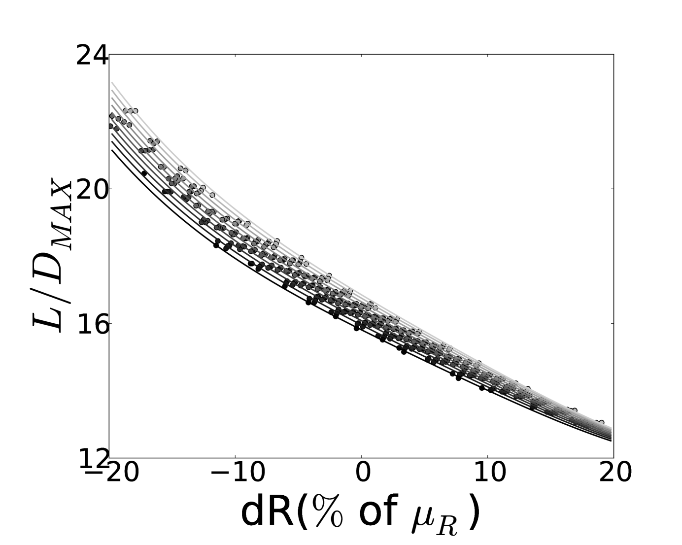
(c) $L/D_{\text{max}}(dR,dS_{r})$

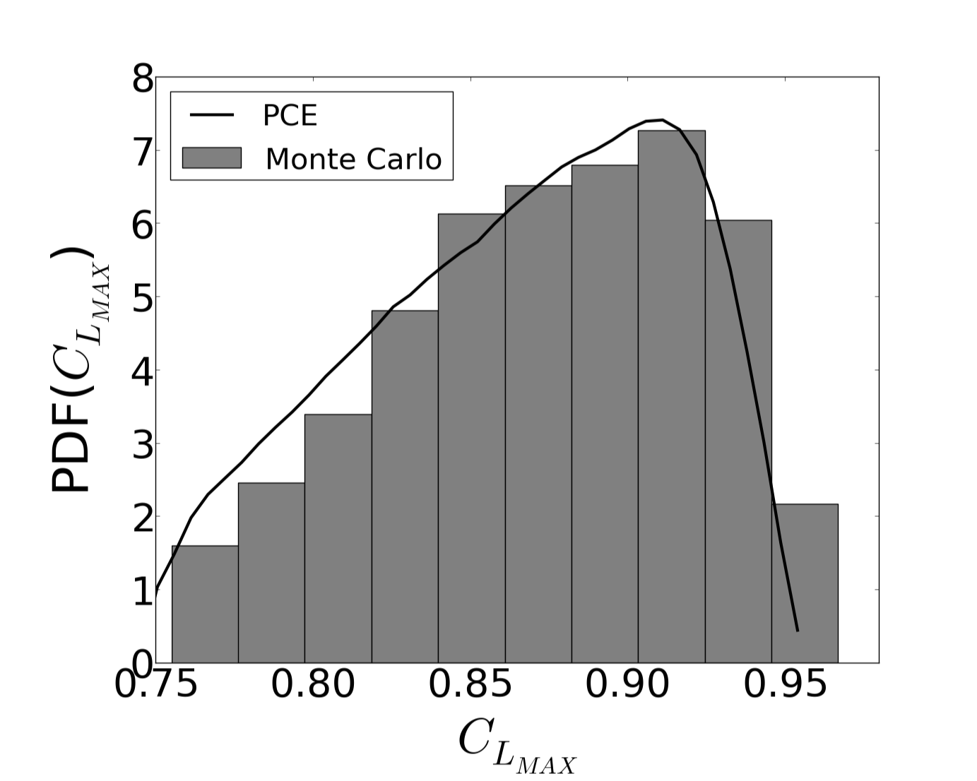
(d) PDF(${C_{L}}_{\text{max}}$)

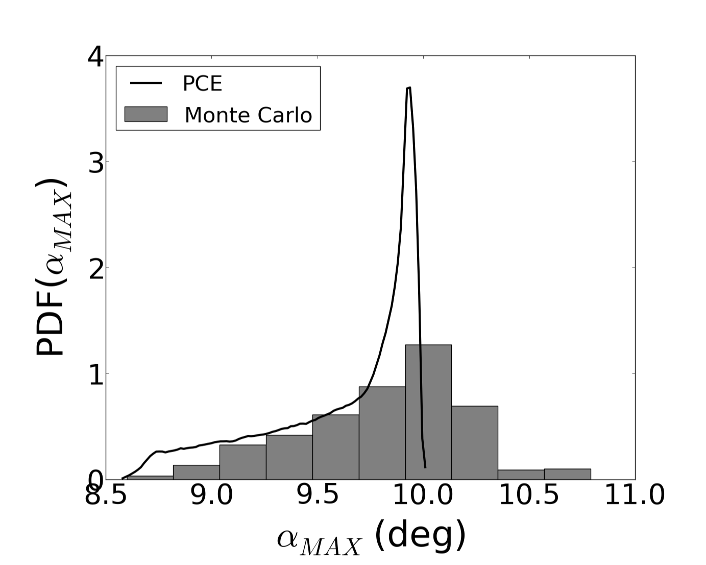
(e) PDF($\alpha_{\text{max}}$)

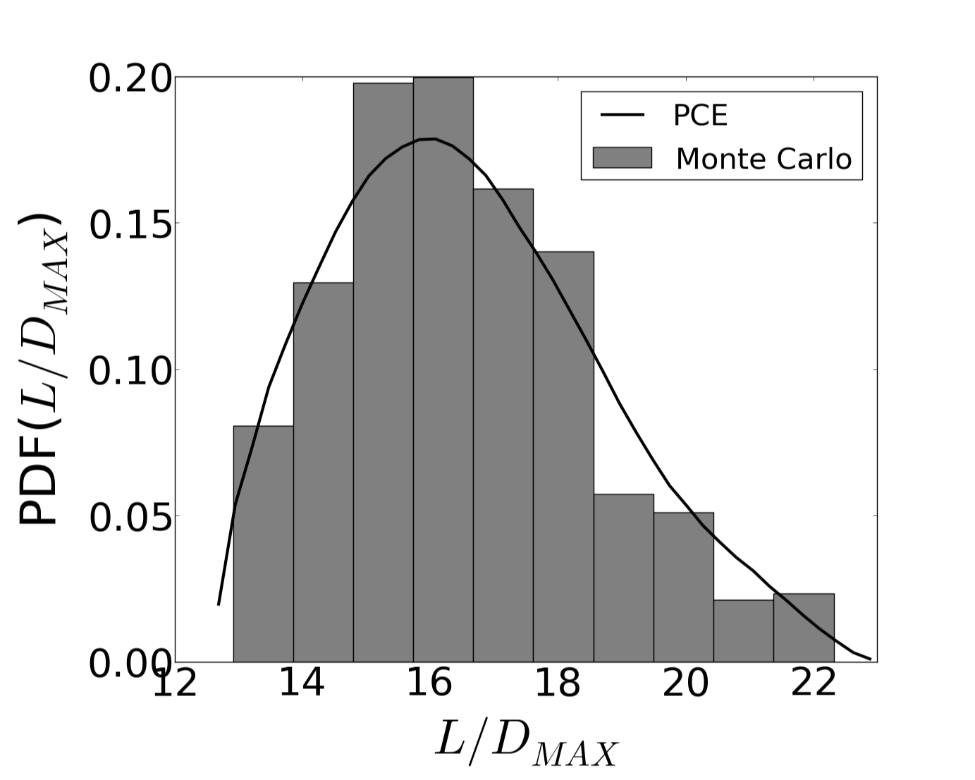
(f) PDF($L/D_{\text{max}}$)

Figure 3: TOP: Comparisons of PCE surrogate maps to Quasi Monte Carlo results. Here $dR$ varies between $\pm 20\%$ of $\mu_{R}$, and $dS_{r}$ varies between $\pm 2.5\%$ of the chord length. The grayscale is chosen to represent different values of $dS_{r}$ (dark to light transition indicates increasing values of $dS_{r}$). The 10 PCE curves in each plot represent values of $dS_{r}$ equally-spaced between $\pm 2.5\%$. BOTTOM: Comparisons of the normalized PDFs for both the Monte Carlo and PCE cases. The input distribution was a Gaussian with $\sigma_{R}$ = 10% of $\mu_{R}$ and $\sigma_{S_{r}}$ = 1.25% of the chord length, with both variables truncated at $2\sigma$.

Table 1: Comparison of Statistical Moments for Monte Carlo and PCE: ($\sigma_{R},\sigma_{S_{r}}$) = (10%,1.25%)

	${C_{L}}_{\text{max}}$			$\alpha_{\text{max}}$ (deg)			$L/D_{\text{max}}$
	MC	PCE		MC	PCE		MC	PCE
Mean	0.87	0.86		9.8	9.6		16.6	16.5
Variance	0.0024	0.0025		0.16	0.13		4.0	4.4
Skewness	$-0.33$	$-0.37$		$-0.50$	$-0.96$		0.56	0.40
Kurtosis	2.3	2.2		2.9	2.7		3.0	2.6

3

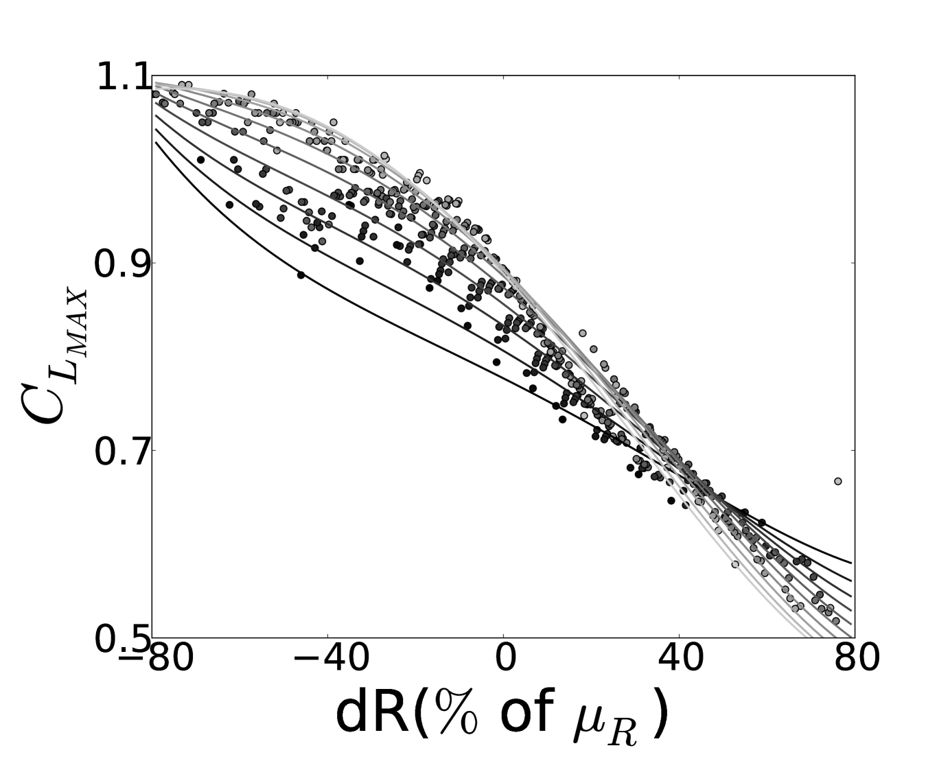
(a) ${C_{L}}_{\text{max}}(dR,dS_{r})$

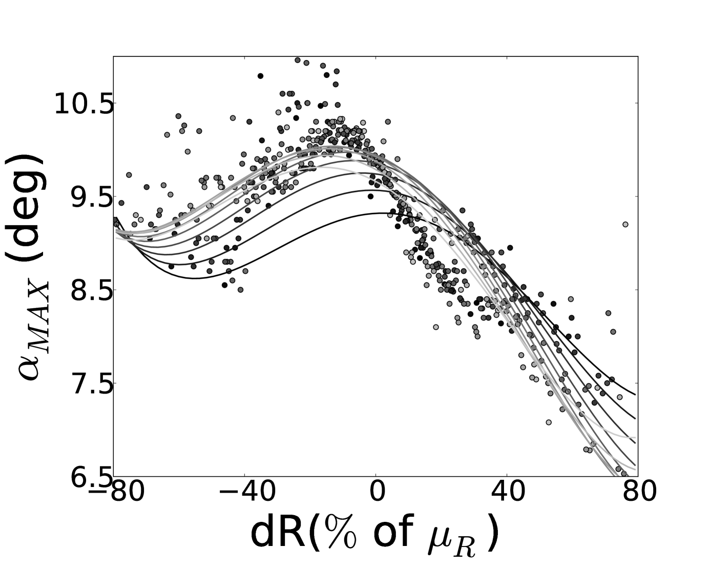
(b) $\alpha_{\text{max}}(dR,dS_{r})$

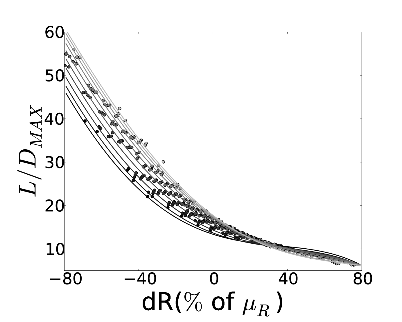
(c) $L/D_{\text{max}}(dR,dS_{r})$

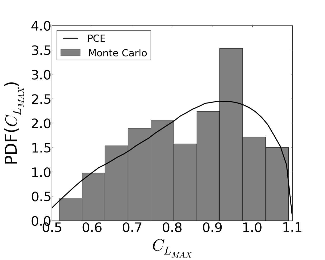
(d) PDF(${C_{L}}_{\text{max}}$)

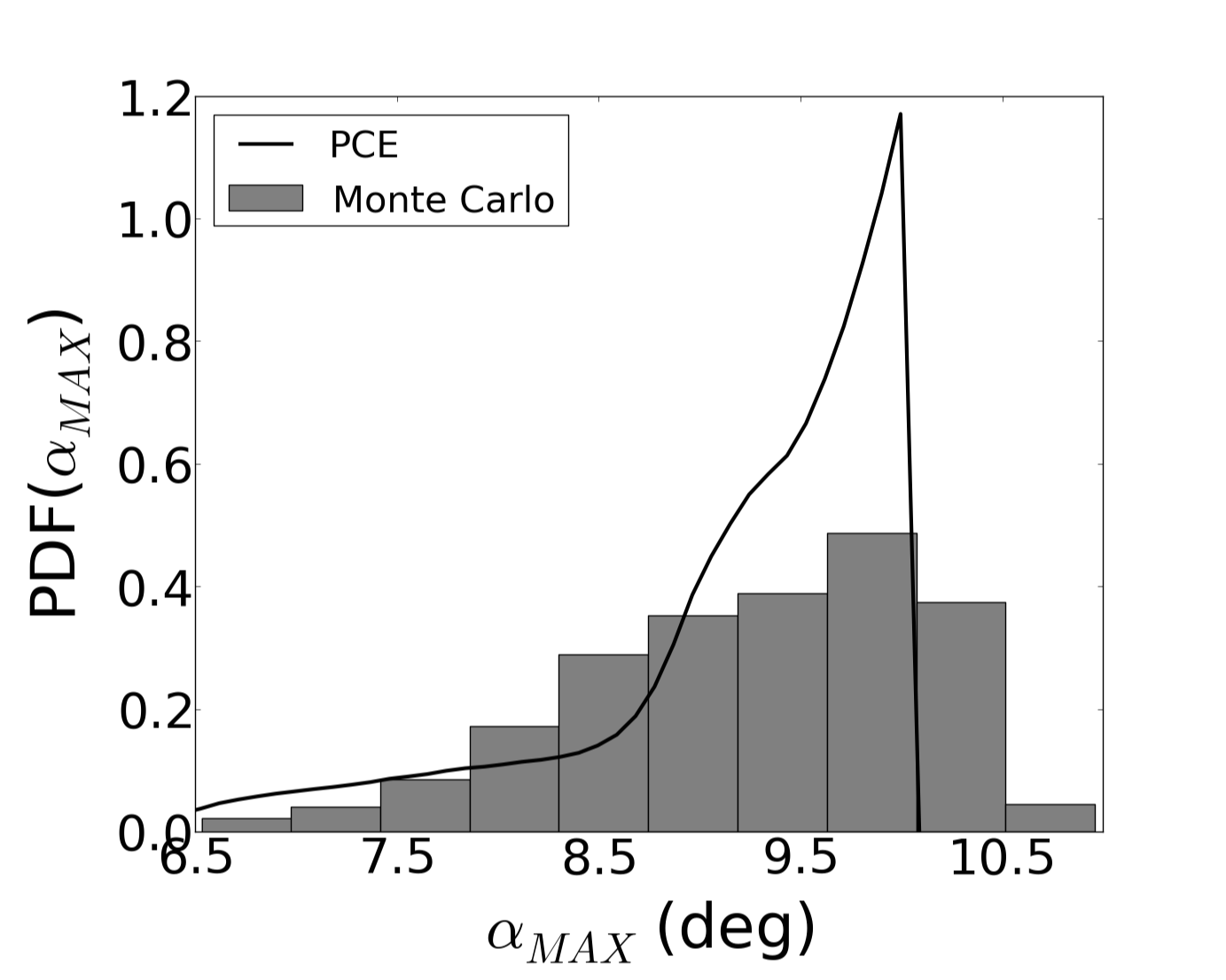
(e) PDF($\alpha_{\text{max}}$)

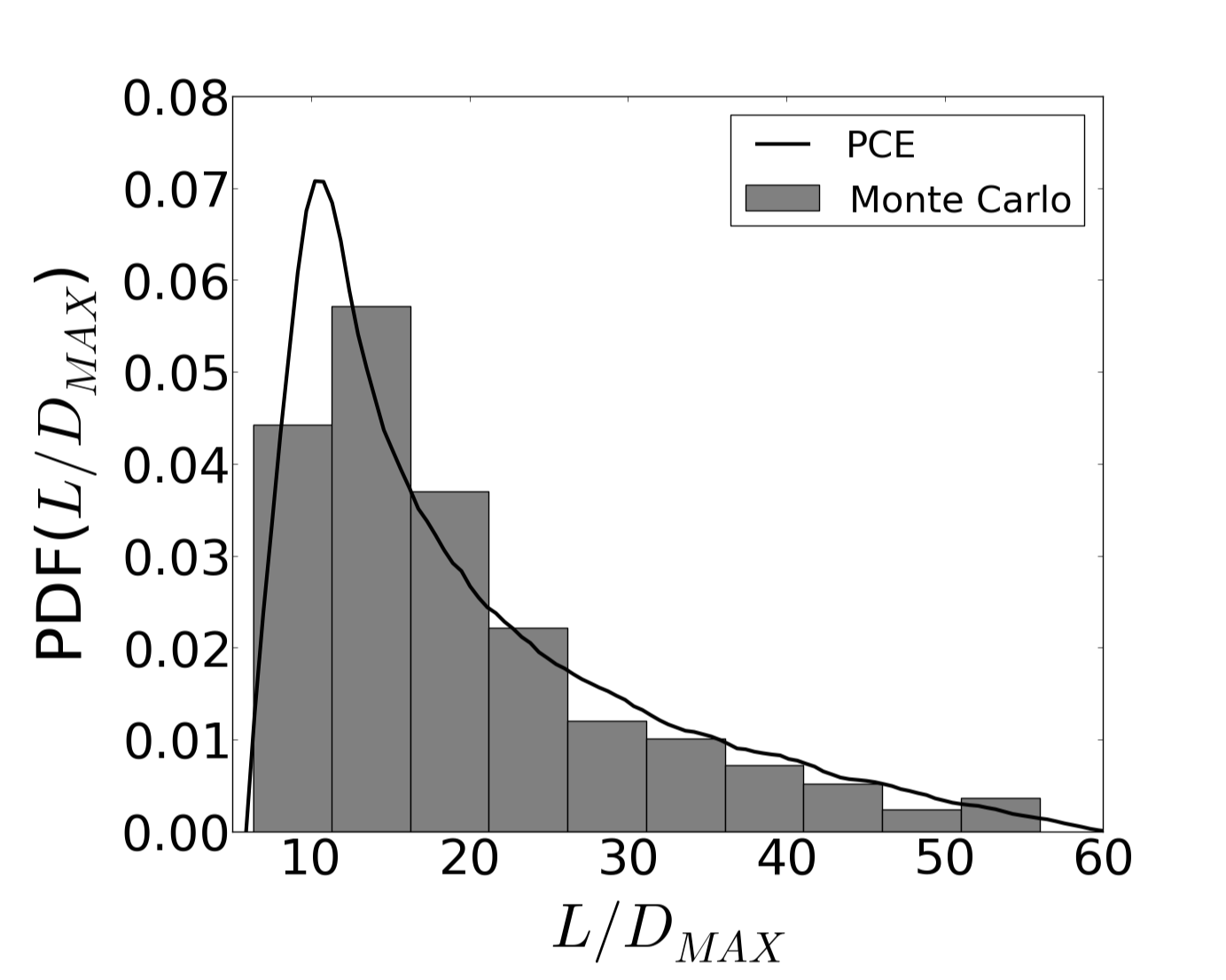
(f) PDF($L/D_{\text{max}}$)

Figure 4: TOP: Comparisons of PCE surrogate maps to Quasi Monte Carlo results. Here $dR$ varies between $\pm 80\%$ of $\mu_{R}$, and $dS_{r}$ varies between $\pm 10\%$ of the chord length. The grayscale is chosen to represent different values of $dS_{r}$ (dark to light transition indicates increasing values of $dS_{r}$). The 10 PCE curves in each plot represent values of $dS_{r}$ equally-spaced between $\pm 10\%$ of the chord length. BOTTOM: Comparisons of the normalized PDFs for both the Monte Carlo and PCE cases. The input distribution was a Gaussian with $\sigma_{R}$ = 40% of $\mu_{R}$ and $\sigma_{S_{r}}$ = 5% of the chord length, with both variables truncated at $2\sigma$.

Table 2: Comparison of Statistical Moments for Monte Carlo and PCE: ($\sigma_{R},\sigma_{S_{r}}$) = (40%,5%)

	${C_{L}}_{\text{max}}$			$\alpha_{\text{max}}$ (deg)			$L/D_{\text{max}}$
	MC	PCE		MC	PCE		MC	PCE
Mean	0.85	0.85		9.2	9.2		19.4	19.7
Variance	0.020	0.022		0.72	0.69		110	120
Skewness	$-0.29$	$-0.38$		$-0.60$	$-1.4$		1.3	1.2
Kurtosis	2.1	2.2		2.9	4.4		4.3	3.7

The top rows of Fig. 3–4 compare the surrogate maps created using the PCE stochastic collocation method to results obtained through Quasi Monte Carlo sampling for ${C_{L}}_{\text{max}}$, $\alpha_{\text{max}}$, and $L/D_{\text{max}}$. The bottom rows present normalized histograms of the Quasi Monte Carlo results and compare them to the results of propagating the input distribution through the PCE surrogate map. The Quasi Monte Carlo method used 500 samples per case, whereas the PCE method utilized 4^th order polynomial expansions and hence required a 5$\times$5 collocation mesh. It should be noted that the Jacobi polynomials—not the Hermite polynomials—were used as the basis in the PCE scheme. There are two reasons for this choice. First, the input distribution in all cases was a truncated Gaussian (i.e., both $dR$ and $dS_{r}$ were truncated at $\pm 2\sigma$). Second, use of the Hermite polynomials might have presented a practical problem, as the collocation nodes tend to lay far out in the tails of the distribution. Sampling at these extreme nodes (corresponding to extreme ridge radii and/or positions) might have presented a problem for the RANS solver. Hence, we used a Jacobi expansion which approximates a truncated Gaussian in distribution and does not require sampling at extreme positions. Specifically, denoting the univariate Jacobi polynomials as $\{J_{i}^{(\alpha,\beta)}\}$, we used the linear expansion $\sum_{i=0}^{5}a_{i}J_{i}^{(2,2)}$ to approximate a truncated Gaussian. See Xiu[9] for an in-depth discussion and for the numerical values of the coefficients $a_{i}$.

Examining the data, we observe that the dominant parameter in all cases is the ridge radius, $R$; the ridge position $S_{r}$ has a relatively smaller effect on the metrics. A larger ridge size (i.e., increasing $dR$) leads to a monotonic decrease in ${C_{L}}_{\text{max}}$ and $L/D_{\text{max}}$. A ridge which is closer to the leading edge (i.e., decreasing $dS_{r}$) also results in a monotonic decrease in ${C_{L}}_{\text{max}}$ and $L/D_{\text{max}}$. This is quite intuitive, since a large ridge radius tends to promote large scale flow separation at lower angles of attack, and a ridge closer to the leading edge disrupts more of the flow over the airfoil.

It is also clear that the agreement between the PCE and Monte Carlo schemes is best for the metrics ${C_{L}}_{\text{max}}$ and $L/D_{\text{max}}$; agreement for $\alpha_{\text{max}}$ is less satisfactory. This can be attributed to the smoothness of the maps. The maps ${C_{L}}_{\text{max}}(dR,dS_{r})$ and $L/D_{\text{max}}(dR,dS_{r})$ are both very smooth—in spectral terms, most of the energy of the PCE expansions which approximate them is contained in the low order modes.

In contrast, $\alpha_{\text{max}}(dR,dS_{r})$ is not as smooth, as can be seen in the Monte Carlo results, particularly at extreme values of $dR$. This reflects a nontrivial amount of energy in higher order spectral terms which are neglected in our 4^th order PCE expansions. However, this should be considered in context with how we obtain the values of $\alpha_{\text{max}}$. Our algorithm for detecting ${C_{L}}_{\text{max}}$ and $\alpha_{\text{max}}$ involves testing the curvature of discrete points on the lift curve—if the curvature exceeds some calibrated bounds, then stall is assumed to have occured, and ${C_{L}}_{\text{max}}$ and $\alpha_{\text{max}}$ are interpolated from the discrete points. As one might expect, this method works well for detecting ${C_{L}}_{\text{max}}$, since that quantity is relatively constant near stall. However, it does not perform as robustly for $\alpha_{\text{max}}$, since that quantity is much more sensitive to perturbations from the true value near stall. Thus, in a sense, we do not even wish to recover the higher order modes for $\alpha_{\text{max}}$, since these reflect the lack of robustness of our algorithm instead of the general trends in the parameter space.

It should also be noted that if greater refinement of the PCE results for $\alpha_{\text{max}}$ is desired, this could be achieved either through retaining higher order terms in the PCE expansion of $\alpha_{\text{max}}$ ($p$-refinement), or through dividing the stochastic space into smaller, discrete elements ($h$-refinement), or a combination of these tactics. In the next section on horn icing, we explicitly demonstrate how to apply stochastic $h$-refinement to improve PCE results.

The effect of an increasing ridge radius on the flowfield is shown in Fig. 5. This figure makes it very clear how different our UQ study is from a sensitivity study, in which the effect of only small perturbations is investigated. In contrast, we are investigating a large amount of uncertainty in ridge size and position, and this leads to a large spectrum of possible flowfields.

3

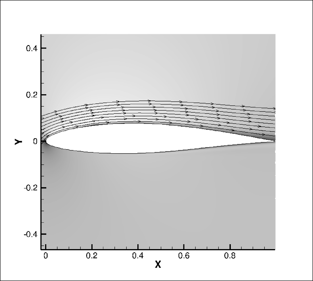
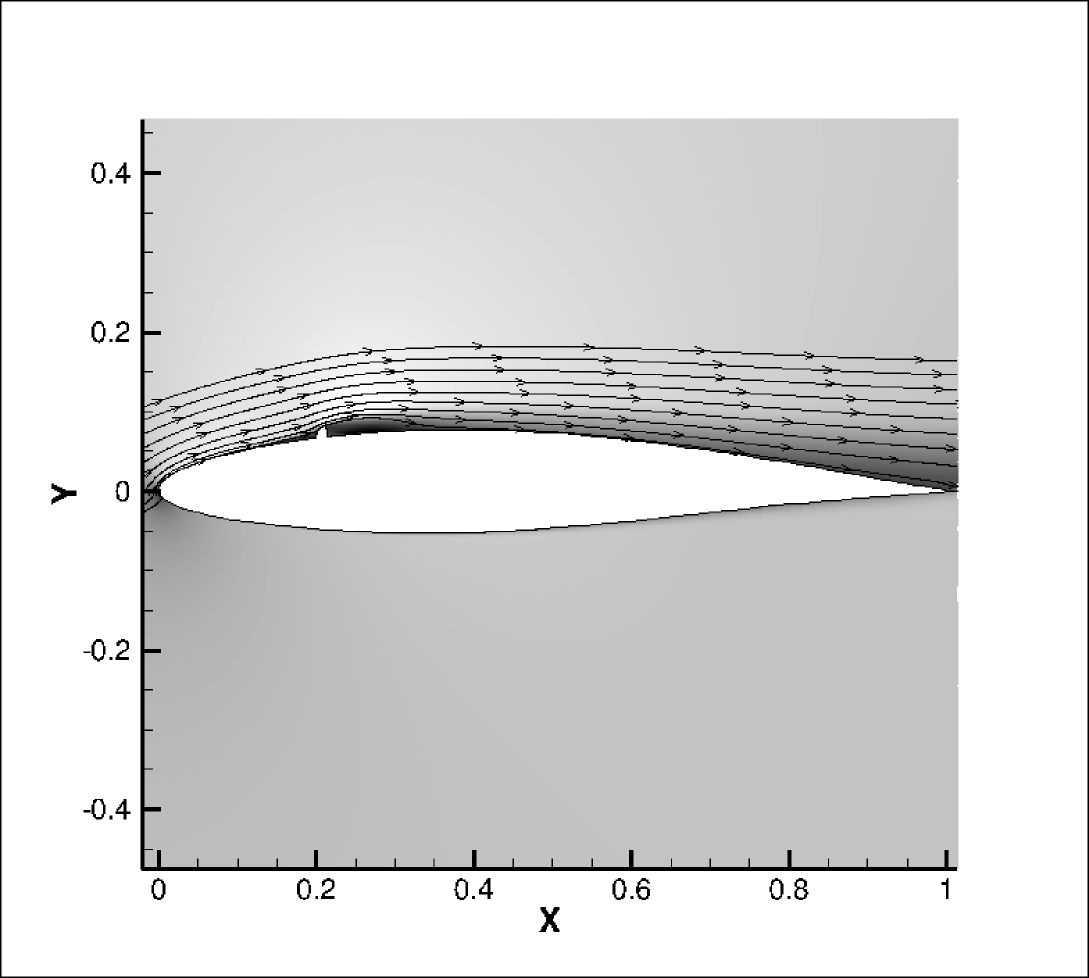
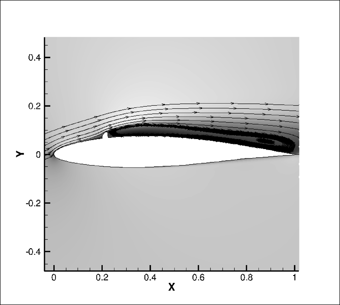
Figure 5: Flow field ($\rho u$) contours for the ridge ice case with increasing ridge radius at $\alpha=6^{\circ}$ in which $dR=-80$, $0$, and $80\%$ of $\mu_{R}$ (going from left to right). The solution for the smallest ridge closely resembles that of the clean airfoil. A large scale separation bubble forms aft of the ridge for the medium sized case before reattaching to the airfoil surface; this separation bubble reduces lift and increases drag. For the large size ridge, the separation bubble caused by the ridge is so large that the flow does not reattach, leading to early stall.

4.2 Horn Ice Case

We approach the horn ice UQ problem in the following way. First, we identify a canonical horn ice shape, which was originally produced by NASA’s LEWICE icing code for 22.5 minutes of ice accretion on a NACA 63A213 airfoil (see Papadakis[10] for more details). That shape is identified in Fig. 1

In our UQ framework, we allow a scaling of the horn height by a parameter which we denote as $h$, with $h\in$ [0,1] (0 corresponds to the clean airfoil, and 1 corresponds to the horn height given in the figure). We also allow a scaling of the inter-horn separation distance by a parameter which we denote as $s$, with $s\in$ [0.1,1.9] (that is, the inter-horn separation distance in the figure can vary by $\pm 90\%$ of its nominal value). We wish to investigate uncertainty in aerodynamic performance metrics given uncertainty in $h$ and $s$, where $h$ is the positive half of the Gaussian $\mathcal{N}(0,0.5^{2})$ (which we will denote as $\mathcal{N}^{+}_{1/2}(0,0.5^{2})$), and $s$ is the Gaussian $\mathcal{N}(1,0.45^{2})$. It should be noted that both parameters are truncated at 2$\sigma$ distance from the mean.

2

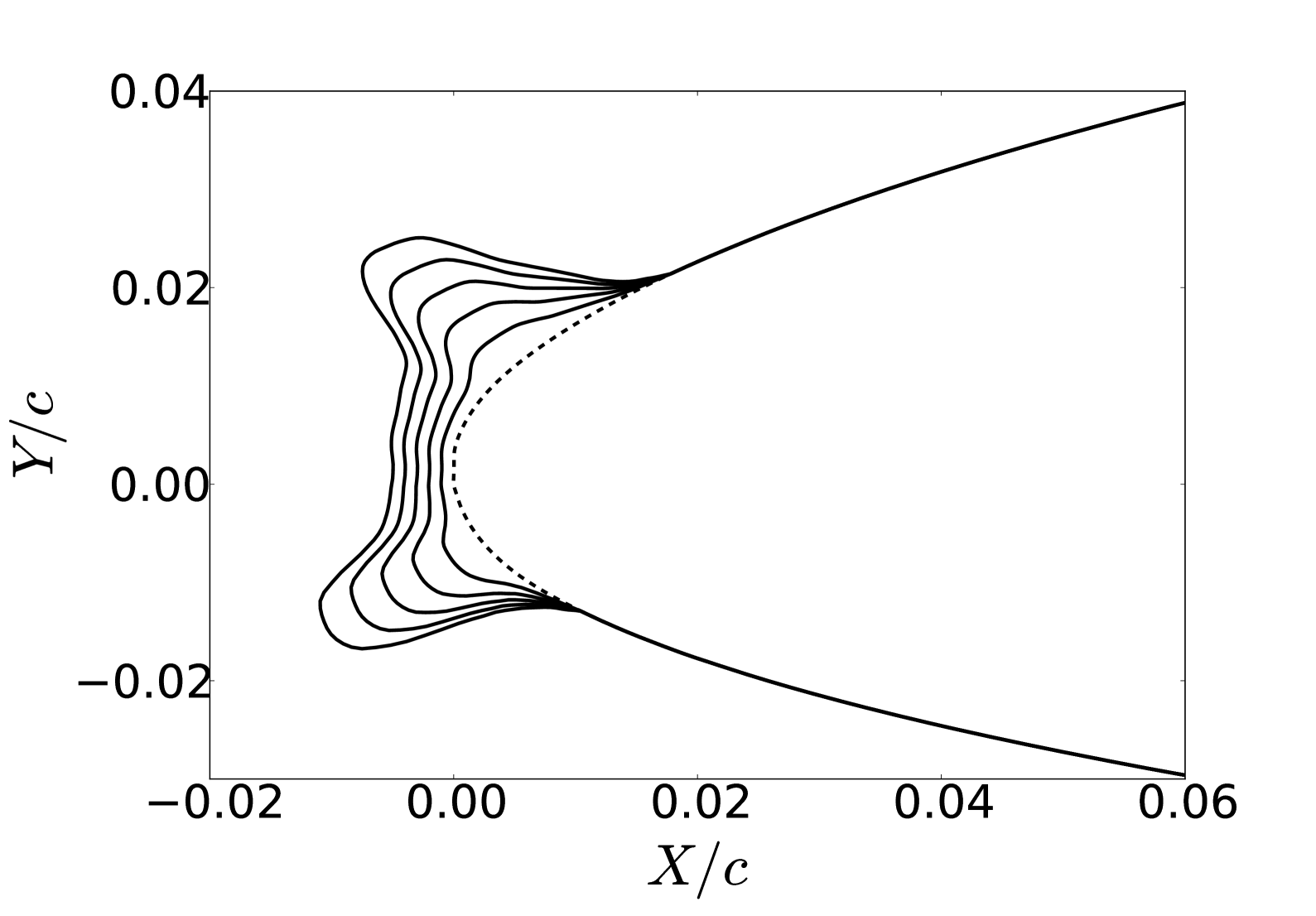
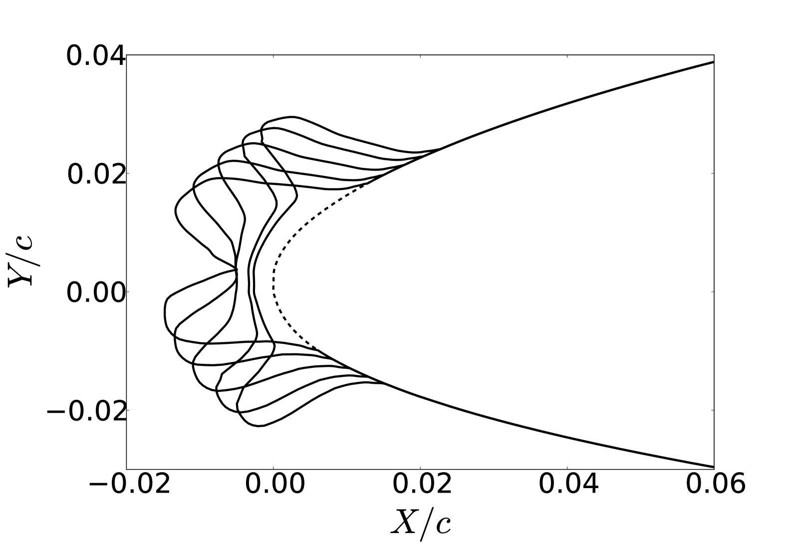
Figure 6: LEFT: Horn shapes produced by variation of the parameter $h\in\{0.2,0.4,0.6,0.8,1\}$ ($s=1$). RIGHT: Horn shapes produced by variation of the parameter $s\in\{0.1,0.5,1,1.5,1.9\}$ ($h=1$).

3

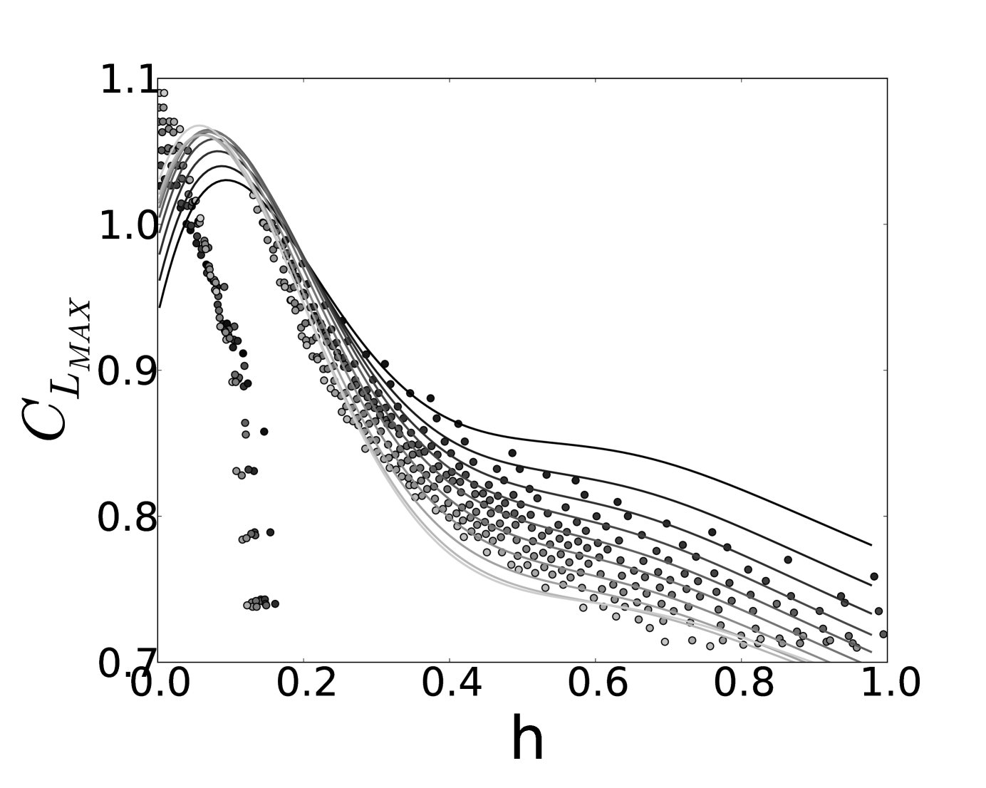
(a) ${C_{L}}_{\text{max}}(h,s)$

(b) $\alpha_{\text{max}}(h,s)$

(c) $L/D_{\text{max}}(h,s)$

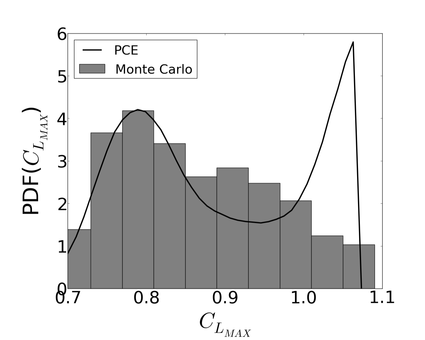
(d) PDF(${C_{L}}_{\text{max}}$)

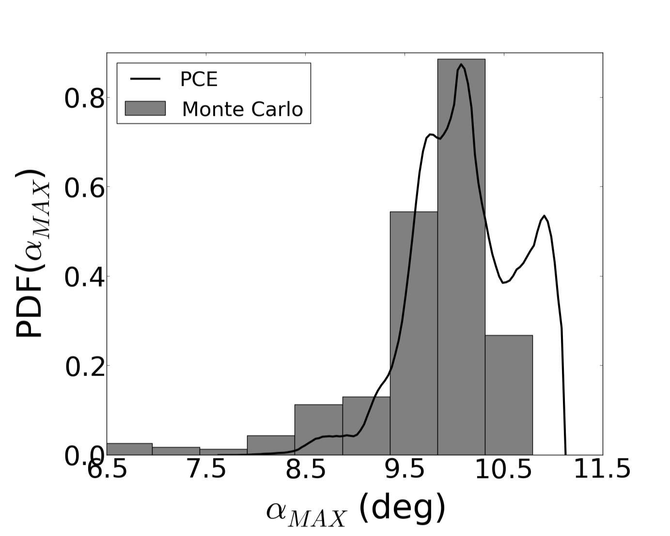
(e) PDF($\alpha_{\text{max}}$)

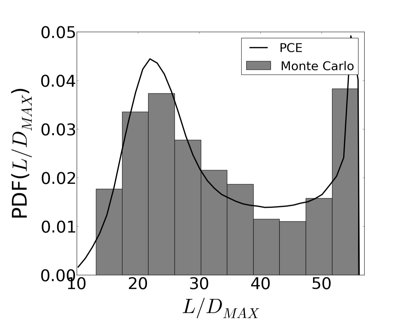
(f) PDF($L/D_{\text{max}}$)

Figure 7: TOP: Comparisons of PCE surrogate maps to Quasi Monte Carlo results (the $s$ axis is going into the page). The range of parameter values is $h\in[0,1]$ and $s\in[0.1,1.9]$. The grayscale is chosen to represent different values of $s$ (dark to light transition indicates increasing values of $s$). The 10 PCE curves in each plot represent values of $s$ equally-spaced in the interval $[0.1,1.9]$. BOTTOM: Comparisons of the normalized PDFs for both the Monte Carlo and PCE cases. The input distributions used were $h$ = $\mathcal{N}_{{1/2}^{+}}(0,0.5^{2})$ and $s=\mathcal{N}(1,0.45^{2})$, with both variables truncated at $2\sigma$.

Table 3: Comparison of Statistical Moments for Monte Carlo and PCE: $h$ = $\mathcal{N}_{{1/2}^{+}}$(0,0.5²), $s$ = $\mathcal{N}$(1,0.45²)

	${C_{L}}_{\text{max}}$			$\alpha_{\text{max}}$ (deg)			$L/D_{\text{max}}$
	MC	PCE		MC	PCE		MC	PCE
Mean	0.86	0.92		9.7	10.2		34	33
Variance	0.0097	0.014		0.84	0.29		170	170
Skewness	0.35	$-0.56$		$-2.3$	$-0.43$		0.38	0.38
Kurtosis	2.1	1.6		8.8	3.1		1.8	1.8

As can be clearly seen in Fig. 7, the dominant parameter is the horn height scale ($h$); variations with horn separation distance ($s$) are smaller by comparison. Unlike the ridge ice cases, there are discontinuities in the maps for both ${C_{L}}_{\text{max}}(h,s)$ and $\alpha_{\text{max}}(h,s)$. The PCE expansions, which are linear combinations of smooth polynomials, obviously cannot resolve such discontinuities. This results in errors in both the PCE surrogate maps and in the output PDFs for ${C_{L}}_{\text{max}}$ and $\alpha_{\text{max}}$. To rectify this issue, we adopt a multi-element approach as suggested by Wan[14].

In this approach, we divide the stochastic space into two separate elements, with the division occuring at the discontinuity ($h$-refinement). We then implement PCE stochastic collocation separately on each of these two elements. This results in piecewise-smooth expansions for ${C_{L}}_{\text{max}}(h,s)$ and $\alpha_{\text{max}}(h,s)$. This results in significantly better agreement between the PCE and Monte Carlo results, as shown in Fig. 8.

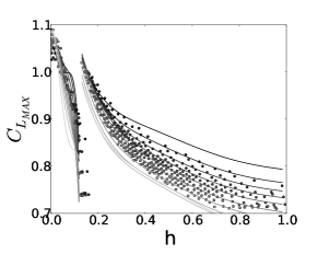
(a) ${C_{L}}_{\text{max}}(h,s)$

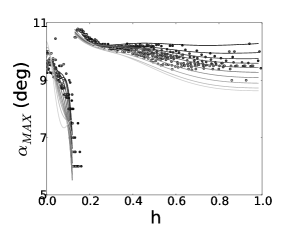
(b) $\alpha_{\text{max}}(h,s)$

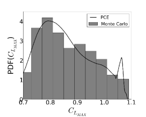
(c) PDF(${C_{L}}_{\text{max}}$)

(d) PDF($\alpha_{\text{max}}$)

Figure 8: TOP: Comparisons of multi-element PCE surrogate maps to Quasi Monte Carlo results. The range of parameter values is $h\in[0,1]$ and $s\in[0.1,1.9]$. The grayscale is chosen to represent different values of $s$ (dark to light transition indicates increasing values of $s$). The 10 PCE curves in each plot represent values of $s$ equally-spaced in the interval $[0.1,1.9]$. BOTTOM: Comparisons of the normalized PDFs for both the Monte Carlo and multi-element PCE cases. The input distributions used were $h$ = $\mathcal{N}_{{1/2}^{+}}(0,0.5^{2})$ and $s=\mathcal{N}(1,0.45^{2})$, with both variables truncated at $2\sigma$.

Table 4: Comparison of Statistical Moments for Monte Carlo and Multi-Element PCE: $h=\mathcal{N}_{{1/2}^{+}}(0,0.5^{2})$, $s=\mathcal{N}(1,0.45^{2})$

	${C_{L}}_{\text{max}}$			$\alpha_{\text{max}}$ (deg)
	MC	MEPCE		MC	MEPCE
Mean	0.86	0.85		9.7	9.9
Variance	0.0097	0.010		0.84	0.71
Skewness	0.35	0.50		$-2.3$	$-2.5$
Kurtosis	2.1	2.3		8.8	9.0

5 Conclusions

Wing icing is not only dangerous to pilots, it is a complex physics problem which is subject to a large amount of uncertainty. Quantifying the exact effects of this uncertainty on airplane performance is hence of great importance to airplane safety.

In this work, we have demonstrated the utility of PCE methods as a fast and accurate method for quantifying the effects on airfoil performance of ice shape uncertainty. The main advantage of our approach is speed and efficiency—each of our PCE results in this paper required only 25 total simulations, compared to the 500 simulations used in the Monte Carlo based schemes (because of the efficiency of Gaussian quadrature). It is our hope that improvements in icing UQ can contribute towards improved safety regulations and protocols for pilots and a mitigation of icing-related accidents.

References

- [1] Landsberg, B., “Aircraft Icing,” Safety Advisor, Weather No. 1, Aircraft Owners and Pilots Association Air Safety Foundation, 2002.
- [2] Wright, W., “User’s Manual for LEWICE Version 3.2,” Tech. Rep. 214255, NASA/CR, 2008.
- [3] Myers, T. G., “Extension to the Messinger Model for Aircraft Icing,” AIAA Journal, Vol. 39, No. 2, 2001.
- [4] Bragg, M. B., Broeren, A. P., and Blumenthal, L. A., “Iced-Airfoil Aerodynamics,” Progress in Aerospace Sciences, Vol. 41, 2005, pp. 323–362.
- [5] Miller, D. R., Addy Jr., H. E., and Ide, R. F., “A Study of Large Droplet Ice Accretions in the NASA-Lewis IRT at Near-Freezing Conditions,” AIAA Paper 96-0934, 1996.
- [6] Hansman, R. J., Yamaguchi, K., Berkowitz, B., and Potapczuk, M., “Modeling of surface roughness effects on glaze ice accretion,” Journal of Thermophysics and Heat Transfer, Vol. 5, No. 1, 1991, pp. 54–60.
- [7] Hansman, R. J. and Turnock, S., “Investigation of Surface Water Behavior During Glaze Ice Accretion,” Journal of Aircraft, Vol. 26, No. 2, 1989, pp. 140–147.
- [8] Ghanem, R. G. and Spanos, P., Stochastic Finite Elements: A Spectral Approach, Springer-Verlag, New York, 1991.
- [9] Xiu, D., Numerical Methods for Stochastic Computations: A Spectral Method Approach, Princeton University Press, 2010.
- [10] Papadakis, M., Gile-Laflin, B. E., Youssef, G. M., and Ratvasky, T. P., “Aerodynamic Scaling Experiments with Simulated Ice Accretions,” AIAA Paper 2001-0833, 2001.
- [11] Tatsumi, S., Martinelli, L., and Jameson, A., “Flux Limited Schemes for the Compressible Navier-Stokes Equations,” AIAA Journal, Vol. 33, No. 2, 1995, pp. 252–261.
- [12] Devroye, L., Non-Uniform Random Variate Generation, Springer-Verlag, New York, 1986.
- [13] Mezic, I., “Uncertainty: Some Conceptual Thoughts and a Good Sampling Method,” USA/South America Symposium on Stochastic Modeling and Uncertainty Quantification, Aug. 2011.
- [14] Wan, X. and Karniadakis, G. E., “An Adaptive Multi-Element Generalized Polynomial Chaos Method for Stochastic Differential Equations,” Journal of Computational Physics, Vol. 209, 2005, pp. 617–642.