Observability of the scalar Aharonov-Bohm effect inside a 3D Faraday cage with time-varying exterior charges and masses

Abstract

In this paper we investigate the scalar Aharonov-Bohm (AB) effect in two of its forms, i.e., its electric form and its gravitational form. The standard form of the electric AB effect involves having particles (such as electrons) move in regions with zero electric field but different electric potentials. When a particle is recombined with itself, it will have a different phase, which can show up as a change in the way the single particle interferes with itself when it is recombined with itself. In the case where one has quasi-static fields and potentials, the particle will invariably encounter fringing fields, which makes the theoretical and experimental status of the electric AB effect much less clear than that of the magnetic (or vector) AB effect. Here we propose using time varying fields $outside$ of a spherical shell, and potentials $inside$ a spherical shell to experimentally test the scalar AB effect. In our proposal a quantum system will always be in a field–free region but subjected to a non-zero time-varying potentials. Furthermore, our system will not be spatially split and brought back together as in the magnetic AB experiment. Therefore there is no $spatial$ interference and hence no shift in a $spatial$ interference pattern to observe. Rather, there arises purely $temporal$ interference phenomena. As in the magnetic AB experiments, these effects are non-classical. We present two versions of this idea: (i) a Josephson temporal interferometry experiment inside a superconducting spherical shell with a time-varying surface charge; (ii) a two-level atom experiment in which the atomic spectrum acquires FM sidebands when it is placed inside a spherical shell whose exterior mass is sinusoidally varying with time. The former leads to a time-varying internal magnetic field, and the latter leads to a time-varying gravitational redshift.

year number number identifier Date text]date

LABEL:FirstPage1 LABEL:LastPage#1

I Introduction

In the 19th century, Faraday showed that when the exterior of a large, enclosed cubical metallic cage (i.e., a “Faraday cage”) is electrified at such a high voltage that sparks started to dart from the corners of the cage, he could still safely conduct many sensitive electrical experiments within the cage, such as sensitive electroscope measurements of the charge residing on the interior surface of the cage. He found the complete absence of any charges residing on the interior surface. Therefore in the special case of a spherical “Faraday cage” configuration, such as the one depicted in Figure 1, one would never expect any kind of electrical effects to be detectable inside the hollow spherical cavity which is carved out of this metallic sphere.

But what is impossible classically is sometimes possible quantum mechanically. For example, a 2D, cylindrical (i.e., tubular) Faraday cage was used in Aharonov and Bohm’s original paper AB effect , in which they first proposed the electric (or “scalar”) Aharonov-Bohm (AB) effect. A metallic tube shielded an electron passing through the tube from any exterior electric fields. However, if a voltage pulse were to be applied to the $exterior$ of the tube only when the electron wavepacket were to be deep in the $interior$ of the tube, then the electron could not feel any forces during its passage through the tube. Nevertheless, the electron would pick up the scalar AB phase shift

$$\varphi(t)=\frac{e}{\hbar}\int_{0}^{t}V\left(t^{\prime}\right)dt^{\prime}$$ (1)

caused by the voltage pulse $V\left(t\right)$ applied to the tube whilst the electron was deep in the interior of the Faraday cage.

The scalar (electric) AB effect is less known than the vector (magnetic) version of the AB effect since it is harder to achieve the situation required for the electric AB effect where fields are vanishing while the potentials are non-zero. If one considers the fields and potentials for the cylindrical Faraday cage used in Aharonov and Bohm’s original paper, then the electron will invariably pass through some region with a non-zero electric field, although the field may be extremely small. To have the electron pass only through regions where there is no field, one needs to switch the fields and potentials on and off completely, i.e., it is necessary to consider the time-dependent fields and potentials described by equation (1), where $V(t)$ is a function with compact support.

The existence of the scalar AB effect has been questioned (see for example the paper by Walstad Walstad ) exactly on the basis that some experimental confirmations of the effect Oudenaarden have the interfering electron passing through regions where the electric field is non-zero, and thus (potentially) one could explain the shift in an interference pattern in terms of classical forces rather than as a quantum phase effect.

In this paper we are proposing two variants of the scalar AB effect as two “thought experiments” which address these questions with setups where a quantum system that is influenced by potentials is always deep inside a field-free region of space. However, since both of these “thought experiments” involve time-dependent potentials which have no spatial gradients, the resulting effect on the system is not a $spatial$ interference phenomenon, as in the vector (magnetic) AB effect, but rather a $temporal$ interference phenomenon.

From equation (1) it can be seen that the phase in the case of the electric AB effect involves just an open time integration as opposed to the usual closed-path spatial line integral of the vector (magnetic) AB effect. This opens the possibility of setting up a scalar AB experiment where one does not split the system along different spatial paths, as in the vector AB setup, but instead the quantum system stays at a single location while the potential will be varying in time. Since we will not be spatially splitting and recombining our system, no $spatial$ interference pattern will result, and therefore no shift in the $spatial$ fringes as in the vector (magnetic) AB effect. However, we shall see below that there can still be a shift in the fringes of a purely $temporal$ interference pattern, or a change of the frequency spectrum of the system.

Our proposal directly tests the scalar AB effect without any “loopholes” that would allow for the effect to be explained any other way. The basic setup involves a spherical metallic shell (i.e., a Faraday cage) that has an oscillating charge $Q\left(t\right)$ or mass $M\left(t\right)$ deposited on it. Inside the shell, the potential is spatially uniform, but is time-varying. The two systems that are placed inside this shell are a Josephson-circuit setup and a two-level atom. In both cases, the interior system does not move spatially and there is a complete absence of any field (electric or gravitational), but the system will experience a time-varying potential energy $U\left(t\right)$ which creates an observable AB effect.

II An electric scalar AB effect via Josephson interferometry

We present here a method to observe the electric scalar AB effect by a superconducting artificial atom Clarke Review ; Makhlin Review . In order to shield the “atom” from external magnetic fields, as shown in Figure 1, it is confined within a superconducting Faraday cage. Internal scalar potential differences arise by sending rf-signals to the surface of the cage. Due to the shielding of the cage, communication between the exterior and interior can only be by way of the scalar AB phase of a Cooper pair, in the limit of electrostatics equilibrium established instantly all over the whole Faraday cage. This assumption satisfies the fact that the skin effect on the surface of the cage doesn’t affect the interior. It may be possible that indications of this internal effect can also be measured by the external circuit.

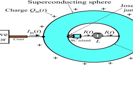
Figure 1: In the spherical superconducting (SC) shell, the SC artificial atom is formed with the hollow cavity and a superconducting wire on the horizontal axis. A SC island is connected to the cavity with a SC wire on one end and via a large Josephson junction on the other end. The effective inductance between the wire and cavity can be enhanced by increasing the number of switchbacks depicted as a solenoid. The spherical SC shell is made thick enough to prevent magnetic flux penetration into interior.

We demonstrate this system by considering the superconducting model circuit of Figure 2. An AC voltage is introduced onto the sphere by charging its self-capacitance. For a superconductor subject to a voltage $V\left(t\right)$, a phase factor $\varphi(t)=\tfrac{2e}{\hbar}\int_{0}^{t}V\left(t\right)dt$ develops within the order parameter of the Cooper pair condensate, $\Psi=\sqrt{\rho}e^{i\varphi}$. Furthermore, a phase difference between the superconducting banks of the Josephson junction also gives rise to a supercurrent according to the inverse AC Josephson effect, i.e. the Levinsen effect Inverse ac JosephsonE . It is therefore possible that the scalar AB phase allows the fully enclosed superconducting circuit to be driven by the external signal generator.

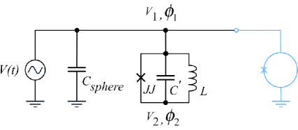
Figure 2: A simplified circuit includes three circuit loops that connected on node 1. In the leftmost loop, a signal generator drives the system. The next loop with the capacitor $C_{sphere}$ represents the spherical SC shell. $C^{\prime}$ and $L$ are the effective capacitance and inductance of the SC island, respectively. The superconducting phase $\varphi_{2}$ on the central superconductor (node 2) and $\varphi_{1}$ on the sphere (node 1) are separated by a Josephson junction modeled with nonlinear inductance $L_{J}$ and effective capacitance $C_{J}$. The right loop demonstrates a simple example of measurement, an rf-SQUID (light blue), although many possible variations of external low-noise readout exist to detect the change of $\varphi_{1}$ in time.

Neglecting possible readout schemes for our model circuit, we construct the Lagrangian using node potentials and phases $\{V_{1},\varphi_{1};V_{2},\varphi_{2}\}$ in the standard way QuantumCircuit ; Devoret . Node phases are related to fluxes by $\varphi_{1,2}=\dfrac{2\pi}{\Phi_{0}}$ $\Phi_{1,2}=\dfrac{2\pi}{\Phi_{0}}\int\mathbf{A}_{1,2}\cdot d\mathbf{x,}$ where flux quanta are $\Phi_{0}=h/2e$. Omitting bias conditions, we find

$$\mathcal{L}\left(\varphi_{2},t\right) =\frac{C_{sphere}}{2}V_{1}^{2}$$

$$\hskip 14.45377pt+\frac{C_{\Sigma}}{2}\left(V_{1}-V_{2}\right)^{2}$$

$$\hskip 14.45377pt-\frac{1}{2L}\left(\Phi_{1}-\Phi_{2}\right)^{2}$$

$$\hskip 14.45377pt+E_{J}\cos\alpha\left(\Phi_{1}-\Phi_{2}\right)$$ (2)

$$=\left(\frac{\hbar}{2e}\right)^{2}\left[\tfrac{1}{2}C_{sphere}\dot{\varphi}_{1}^{2}\right.$$

$$\hskip 14.45377pt+\frac{C_{\Sigma}}{2}\left(\dot{\varphi}_{2}-\dot{\varphi}_{1}\right)^{2}$$

$$\hskip 14.45377pt-\frac{1}{2L}\left(\varphi_{2}-\varphi_{1}\right)^{2}$$

$$\hskip 14.45377pt\left.+E_{J}\cos\left(\varphi_{2}-\varphi_{1}\right)\right]$$ (3)

Considering $V_{1}$ is driven $\left(V_{1}=V_{0}\sin\omega t\right)$, the interior phase $\Delta\varphi=\varphi_{2}-\varphi_{1}$ and $\Delta\dot{\varphi}=\dot{\varphi}_{2}-\dot{\varphi}_{1}$ become the independent variables in the Lagrangian. This allows us to get the following equation of motion with driving on $\dot{\varphi}_{1}$.

$$0 =\Delta\ddot{\varphi}+\omega_{C}^{2}\Delta\varphi+\left(\frac{2e}{\hbar}\right)^{2}\frac{E_{J}}{C_{\Sigma}}\sin\Delta\varphi$$

$$\hskip 14.45377pt+\left(\frac{2e}{\hbar}\right)^{2}\frac{C_{g}V_{0}\omega}{C_{\Sigma}}\cos\omega t$$ (4)

where $\Delta\varphi=\left(\varphi_{2}-\varphi_{1}\right)$, $\omega_{C}=\dfrac{1}{LC^{\prime}}$. Here $C_{g}$ is the effective gate capacitance of the SC island and $C_{\Sigma}$ is the total capacitance of the system. We adopt the following initial conditions, which assume an initial steady state throughout the system.

$$\left\{\begin{array}[c]{c}\varphi_{2}\left(t=0\right)=\varphi_{1}\left(t=0\right)\\ \dot{\varphi}_{2}\left(t=0\right)=\dot{\varphi}_{1}\left(t=0\right)\end{array}\right.$$ (5)

Figure 3 depicts the calculated dynamics of $\Delta\varphi$. When the floating part node 2 is initially grounded and the internal circuit is cooled down to ground state, a signal of $V_{1}$ drives $\Delta\varphi$ starting at some moment according to the equation of motion (4). Hence an interior supercurrent is being driven after the signal is turned off at some point and causes a nonvanishing $\Delta\varphi$ because of the Josephson effect, which reflects on changing $\varphi_{1}$ from the internal circuit. An rf-SQUID (light blue in Figure 2) at the read out port picks up the time dependent phase $\varphi_{1}$ and converts it into time dependent magnetic flux which can be detected from an exterior circuit. We have therefore demonstrated that the external generator affects the fully enclosed superconducting circuit.

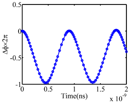
Figure 3: Phase difference across JJ $\Delta\varphi$ in terms of tme, solved from the Lagrangian equation of motion, when $\omega_{0}\approx 8.5GHz,\alpha\approx 2\times 10^{-15}Wb,V_{0}=1\mu V,\omega=150MHz.$

Also notice that the internal Josephson junction circuit, with the possible addition of current or flux biasing, shares a similar circuit topology to phase or flux qubits, respectively Phase qubit ; Flux qubit . In any case, when $E_{J}\gg E_{C}=\tfrac{\left(2e\right)^{2}}{2C_{\Sigma}}$, phase is a good quantum number. The anharmonic potential energy, $U\left({\Delta\varphi}\right)=\left({\tfrac{\hbar}{{2e}}}\right)^{2}\tfrac{1}{{2L}}\left({\Delta\varphi}\right)^{2}-E_{J}\cos\left({\Delta\varphi}\right)$ is depicted as in Figure 4 and gives quantized energy levels similar to an atom occupying the local minimas of this periodic potential. This artificial atomic system, as we have just determined, is affected by the external modulating voltage. Note that the electric potential becomes $\partial/\partial\varphi$ which is the conjugate variable of ${\Delta\varphi}$ in the Hamiltonian. Driving on the potential could displace the phase from ${\Delta\varphi=0}$ to ${\Delta\varphi=2\pi}$. A $2\pi$ phase in the internal circuit corresponds to a flux quantum in the cavity generated by the persistent current going through the central SC wire. After releasing the driving, the system may stay in the ${\Delta\varphi=2\pi}$ state until there is a relaxation back to ${\Delta\varphi=0}$, which can be detected via measurement of the rf-SQUID (rightmost loop in Figure 2). If the driving finishes one cycle from ${\Delta\varphi=0}$ to ${\Delta\varphi=0}$, the magnetic flux quantum comes back to zero in the cavity. Therefore, the internal magnetic flux becomes the consequence of a temporal scalar AB effect.

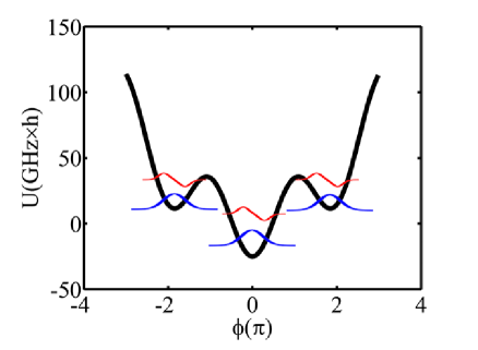
Figure 4: A plot of potential energy for $E_{L}=1GHz\times h,E_{J}=25GHz\times h.$ Blue is the ground state for each well while red is the first excited state. Inter-well tunneling may occur, in which microwave photons may be emitted or absorbed.

Here we make the following observations:

(1) The supercurrent is created due interference between two paths for the propagation of the SC phase to node-2. One of the paths is via the JJ and the other is via the solenoid.

(2) The scalar AB phase discussed here is only for a single Cooper pair instead of a bulk system. As pointed out earlier, the phase difference drives the supercurrent that in principle can be detected. Considering the bulk system, the AB phase factor should include the phase from all Cooper pairs, $\varphi_{C.P.}\left(t\right)=\frac{2e}{\hbar}\int_{0}^{t}N_{C.P.}\left(t\right)V\left(t\right)dt$, and electrons,$\ \varphi_{els}\left(t\right)=\frac{e}{\hbar}\int_{0}^{t}N_{els}\left(t\right)V\left(t\right)dt$. Here $N_{C.P.}\left(t\right)$ is the total number of Cooper pairs (which is not conserved in principle) and $N_{els}\left(t\right)$ is the total number of electrons of the whole system. Also, AB phase factor from ionic lattice should be included as well $\varphi_{ion}\left(t\right)=\frac{-e}{\hbar}\int_{0}^{t}N_{ion}\left(t\right)V\left(t\right)dt$. For the case of a 3D rf-SQUID confined within the Faraday cage (see Figure 1), there will arise time-varying charge imbalances between the charge of the fixed ionic lattice and the charge of the mobile Cooper pairs on the SC island, which will give rise to a nonzero total AB phase developed in the internal circuit. The AB effect here merely drives the Cooper pair condensate and generates a magnetic field in the internal cavity. This is the physical reaction caused by the scalar AB phase that we expect here by theoretical analysis.

(3) Driving the SC atom away from ${\Delta\varphi=0}$ to ${\Delta\varphi=2}\pi$ becomes analogous to the case of the ionization of an atom. Consequently, we can expect that treating this perturbation results in a nonlocal photoelectric effect.

III A gravitational AB phase shift observable as a time-dependent gravitational redshift

Here we consider the problem of a two-level atom that is undergoing a time-dependent gravitational redshift when the atom is placed inside a time-varying spherical mass shell $M(t)$ (see Figure 5) Again, as in the electric case, the gravitational scalar potential will be uniform everywhere within the interior of a mass shell, so that no gravitational force will be experienced by the atom. Nevertheless, there can in general arise a scalar AB phase Hohensee , which arises from the Newtonian gravitational scalar potential $\Phi$

$$\varphi\left(t\right)=\frac{1}{\hbar}\int_{0}^{t}m\left(t^{\prime}\right)\Phi\left(t^{\prime}\right)dt^{\prime}$$ (6)

where $m\left(t^{\prime}\right)$ is the time-varying rest mass of the quantum system that is acquiring this phase shift. The Newtonian gravitational scalar potential for a time-varying mass shell $M\left(t\right)$, such as that associated with the sinusoidally time-varying charge $Q\left(t\right)$ on the surface of the shell depicted in Figure 1, is given by

$$\Phi\left(t\right) =-\frac{GM\left(t\right)}{r_{0}}$$

$$=-\frac{G\left(M_{0}+M_{1}\cos\omega t\right)}{r_{0}}$$ (7)

where $G$ is Newton’s constant, $r_{0}$ is the radius of the mass shell, $M_{0}$ is the DC component of the mass shell, and $M_{1}$ is the amplitude of the AC component of the time-varying mass shell. It goes without saying that the mass-to-charge ratio of the electron is so tiny that the AC component associated with $M_{1}$ will be extremely small, so that there would be no hope for any practical laboratory experiment in connection with the Faraday cage configuration shown in Figure 5. However, we are concerned here with the problem of whether in principle the gravitational AB phase exists or not, so that a “thought experiment” would suffice here.

Nevertheless, there exist astrophysical situations, such as in the case of an exploding mass shell of a supernova, where the radius $r_{0}\left(t\right)$ is the time-dependent quantity rather than the mass $M\left(t\right)$. Then the gravitational AB phase shift may be large enough to be seen in practice. In any case, although the gravitational scalar potential may vary with time, nevertheless it must be independent of the position of the field point within the interior of the mass shell. This follows from Gauss’s theorem. Therefore the atom within the mass shell experiences no classical forces. However, it can experience a nonzero quantum phase shift arising from the gravitational AB effect.

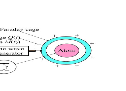
Figure 5: Two-level atom inside a spherical mass shell with a time-dependent mass $M(t)$ that arises from a time-dependent charge $Q(t)$. The mass $M(t)$ results a time-dependent gravitational redshift that leads to observable FM sidebands in the spectrum of the atom.

The rest mass of the excited state of an atom or of a nucleus will be larger than the rest mass of the ground state of this atom or nucleus. This follows from Einstein’s equation

$$E=mc^{2}$$ (8)

In quantum mechanics, Einstein’s equation becomes

$$mc^{2}=\left\langle\psi\left(t\right)\right|i\hbar\frac{\partial}{\partial t}\left|\psi\left(t\right)\right\rangle$$ (9)

Thus the rest mass $m$ in relativity is the expectation value of the energy operator $i\hbar\partial/\partial t$ in quantum mechanics. For example, when an atom is in a stationary state $\left|\psi\left(t\right)\right\rangle=\left|\Psi_{E}\right\rangle\exp\left(-iEt/\hbar\right)$, it follows from (9) that

$$mc^{2}=E\left\langle\Psi_{E}\right.\left|\Psi_{E}\right\rangle=E$$ (10)

and thus we recover Einstein’s equation (8). We shall assume that (9) holds in general for open quantum systems, such as that of an atom inside a time-varying mass shell depicted in Figure 5.

Now from the expression for the gravitational AB phase (6), we expect that the atom in a stationary state with an energy $E$ inside the mass shell will pick up an AB phase factor, so that

$$\left|\psi\left(t\right)\right\rangle=\left|\Psi_{E}\right\rangle\exp\left(-iEt/\hbar\right)\exp\left(-i\varphi\left(t\right)\right)$$ (11)

Substituting this into (9), we find

$$mc^{2}=\left\langle\Psi_{E}\right|\{E+\hbar\dot{\varphi}\}\left|\Psi_{E}\right\rangle=E+\hbar\dot{\varphi}$$ (12)

which is an application of (9) to the case of a time-dependent environment, such as the time-varying mass shell. To find $\dot{\varphi}$, let us take the time derivative of the expression for the AB phase (6). Then one obtains the relationship

$$\dot{\varphi}=\frac{1}{\hbar}m\left(t\right)\Phi\left(t\right)$$ (13)

The physical meaning of this relationship is that the “instantaneous” frequency $\dot{\varphi}$ associated with the modulation of the phase of the atomic wavefunction due to an “instantaneous” change in the gravitational potential energy $m\left(t\right)\Phi\left(t\right)$ of the atom inside the mass shell, leads to an ”instantaneous” energy change of the energy level of the atom given by

$$\delta E=\hbar\dot{\varphi}=m\left(t\right)\Phi\left(t\right)$$ (14)

Upon substitution of $\dot{\varphi}$ from (13) back into (12), it follows that

$$mc^{2}=E+m\left(t\right)\Phi\left(t\right)$$ (15)

from which we infer that

$$E=mc^{2}\left(1-\frac{\Phi}{c^{2}}\right)$$ (16)

which leads to the conclusion that the rest mass of quantum mechanical systems may be increased due to its external gravitational environment.

If we now take the difference in the upper and lower energy levels of the two-level atom and set it equal to the frequency of an emitted photon $f_{0}$ times Planck’s constant $h$, we will find that

$$hf_{0}=hf\left(1-\frac{\Phi}{c^{2}}\right)$$ (17)

Since $\Phi$ is a negative quantity, this implies that the photon of energy $hf$ as seen by an observer at infinity will be smaller in energy than the photon of energy $hf_{0}$ as seen by an observer near to the atom. Thus we have recovered Einstein’s gravitational redshift starting from the gravitational AB phase shift.

Now if the potential $\Phi$ were to be time varying due to changes in the mass shell, the gravitational red shift would be changed by the time variation of $\Phi$. If the time variation were to be sinusoidal, then we would expect the emission and absorption spectrum of the atom to undergo FM modulation. To see this, let us assume that the states of a two-level atom are represented by $\left|i\right\rangle$ for the initial state and by $\left|f\right\rangle$ for the final state. Then Fermi’s Golden Rule states that the rate of transitions $w_{f\leftarrow i}$ between these two states will be given by the absolute square of the transition matrix element connecting the initial and final states, i.e.,

$$w_{f\leftarrow i}\propto\left|\left\langle f\right|H^{\prime}\left|i\right\rangle\right|^{2}$$ (18)

where $H^{\prime}$ is the time-dependent perturbation that causes the transitions to occur. (For the present purposes, we ignore the proportionality constant and the density of final states in Fermi’s Golden Rule.)

Let us first consider the effect of the $electric$ scalar AB effect on the transitions between the initial and final states of a $charged$ atom, i.e., an ion, within the spherical shell of the Faraday cage. The electric AB phase is given by

$$\varphi_{q}\left(t\right)=\frac{q}{\hbar}\int_{0}^{t}V\left(t^{\prime}\right)dt^{\prime}$$ (19)

where $q$ is the charge of the ion. Since the initial and final states of the transition must have the same charge $q$ (which follows from Wigner’s charge superselection rule), it follows that the electric AB phase factors in the transition matrix elements in Fermi’s Golden Rule must cancel out, i.e.,

$$w_{f\leftarrow i} \propto\left|\left\langle f\right|e^{+i\varphi_{q}(t)}H^{\prime}e^{-i\varphi_{q}(t)}\left|i\right\rangle\right|^{2}$$

$$=\left|\left\langle f\right|H^{\prime}\left|i\right\rangle\right|^{2}$$ (20)

since $[H^{\prime},V\left(t\right)]=0$. From (20), we conclude that the electric AB effect cannot be observed in the spectroscopy of any charged atomic system.

However, this is $not$ true for the gravitational AB effect. This is because of the fact that the $rest$ $mass$ of an excited atom will be greater than the $rest$ $mass$ of the unexcited atom. (Recall that there exists no superselection rule for mass, unlike for the case of charge.)

Now from Einstein’s equation (8), it follows that there exists a rest mass difference between the final and the initial states of the two-level atom, which is given by

$$\Delta m=\frac{\Delta E}{c^{2}}=\frac{E_{f}-E_{i}}{c^{2}}$$ (21)

where $E_{f}$ is the energy level of the final state and $E_{i}$ is the energy level of the initial state. Therefore from (6), we see that the difference in the gravitational AB phase picked up by the final state and the phase picked up the initial state will no longer vanish, but will differ by the amount

$$\Delta\varphi\left(t\right) =\frac{\Delta m}{\hbar}\int_{0}^{t}\Phi\left(t^{\prime}\right)dt^{\prime}$$

$$=\frac{E_{f}-E_{i}}{\hbar c^{2}}\int_{0}^{t}\Phi\left(t^{\prime}\right)dt^{\prime}$$ (22)

where, to a a first approximation, the energy difference $E_{f}-E_{i}$ is independent of $\Phi$.

As a simple example of how the difference in the gravitational AB phases in the initial and final states can lead to an observable AB interference effect, let us consider a superposition of the initial and final states which is initially given by

$$\left|\Psi\left(t=0\right)\right\rangle\propto\left|i\right\rangle+\left|f\right\rangle$$ (23)

After a time $t=T$, this superposition will evolve to pick up phase factors, viz.,

$$\left|\Psi\left(t=T\right)\right\rangle \propto\left|i\right\rangle e^{-\frac{i}{\hbar}E_{i}T}e^{-i\varphi_{i}T}$$

$$+\left|f\right\rangle e^{-\frac{i}{\hbar}E_{f}T}e^{-i\varphi_{f}T}$$ (24)

where

$$\varphi_{i}\left(T\right)=\frac{E_{i}}{\hbar c^{2}}\int_{0}^{T}\Phi\left(t^{\prime}\right)dt^{\prime}$$ (25)

$$\varphi_{f}\left(T\right)=\frac{E_{f}}{\hbar c^{2}}\int_{0}^{T}\Phi\left(t^{\prime}\right)dt^{\prime}$$ (26)

are the gravitational AB phases picked up by the initial and final states, respectively. From (22) and (24) it follows that

$$\left|\Psi\left(t=T\right)\right\rangle\propto\left|i\right\rangle+\left|f\right\rangle e^{-\frac{i}{\hbar}\left(E_{f}-E_{i}\right)T}e^{-i\Delta\varphi T}$$ (27)

where $\Delta\varphi\left(T\right)=\varphi_{f}\left(T\right)-\varphi_{i}\left(T\right)$ is the difference of the two AB phases. From (6) and (7), we see that

$$\varphi_{i}\left(T\right)=\alpha_{i}\sin\omega t$$ (28)

$$\varphi_{f}\left(T\right)=\alpha_{f}\sin\omega t$$ (29)

where $\alpha_{i}=GM_{1}m_{i}/\hbar\omega r_{0}$ and $\alpha_{f}=GM_{1}m_{f}/\hbar\omega r_{0}$ are the FM modulation parameters for the initial and final wavefunctions, respectively, of the two-level atom. The sinusoidal modulations of the phases given by (28) and (29) will lead to many FM harmonics of the frequency $\omega$ via the Jacobi-Anger expansion of the wavefunctions of the two-level atom (see Appendix A). For large values of $\alpha_{i}$ and $\alpha_{f}$, the dominant upper and lower FM sidebands of the FM-modulated wavefunctions of the atom will occur at the frequency shifts $\pm\alpha_{i}\omega$ and $\pm\alpha_{f}\omega$ away from their usual frequencies of $E_{i}/\hbar$ and $E_{f}/\hbar$.

It follows that the usual energy-conservation-enforcing delta function in the Fermi Golden rule will be modified from the usual two-level atom resonance condition not only by the usual gravitational red shift stemming from the DC component of the mass shell $M_{0}$, but it will also be modified due to the FM sidebands that arise from the AC component of the time-varying mass shell $M\left(t\right)$. The bottom line of this analysis is that the usual absorption or emission line of the two-level atom will be split into upper and lower FM sideband frequencies occurring on either side of the unsplit line of the atom with frequency shifts of $\pm(\Delta\alpha)\omega$, where

$$\Delta\alpha =\left(\alpha_{f}-\alpha_{i}\right)$$

$$=\frac{GM_{1}\left(m_{f}-m_{i}\right)}{\hbar\omega r_{0}}$$ (30)

is the difference between the FM modulation parameters of the final state and the initial state that stems from the difference in their rest masses, $m_{f}-m_{i}$.

IV Conclusions

We conclude from the above two “counter-examples” that the claims of the non-existence of the scalar AB effect are false. Although these two “counter-examples” are by nature merely “thought experiments,” they do establish the $existence$ of the electric AB effect and the $existence$ of the gravitational AB effect in principle. However, they may ultimately lead to actual experiments in the laboratory in the Josephson interferometry case, and to actual observational evidence in astrophysical settings in the gravitational redshift case.

Finally, we note that the magnetic (vector) AB effect as observed by Tonomura Tonomura using ferromagnetic toroids in electron interference experiments, are obviously topological in nature. However, the electric and gravitational (scalar) AB effects that are predicted to occur here inside the metallic shells of Figures 1 and 5, are obviously non-topological in nature.

V Appendix A: Bloch’s theorem for scalar potentials that are periodic in time

Consider the general case in which the potential energy inside the Faraday cages depicted in Figures 1 and 5 satisfy the periodicity condition in time

$$U\left(t+T\right)=U\left(t\right)$$ (31)

where the period $T=2\pi/\omega$ is that of an arbitrary periodic waveform generator that replaces the sine-wave generators in Figures 1 and 5. Then it is apparent that this temporal periodicity condition is mathematically identical to the spatial periodicity condition

$$U\left(x+a\right)=U\left(x\right)$$ (32)

that applies to a 1D crystalline lattice with a lattice constant $a$.

Bloch’s theorem Kittel then tells us that the wavefunction inside the 1D crystalline lattice is given by

$$\psi\left(x\right)=e^{ipx/\hbar}u_{p}\left(x\right)$$ (33)

where $p$ is the “crystal momentum” or “quasi-momentum”, and where

$$u_{p}\left(x+a\right)=u_{p}\left(x\right)$$ (34)

is a periodic function of $x$ within the spatial crystalline lattice.

Similarly, the temporal version of Bloch’s theorem (also known as “Floquet’s theorem”) is given by

$$\psi\left(t\right)=e^{-iEt/\hbar}u_{E}\left(t\right)$$ (35)

where $E$ is the “crystal energy” or “quasi-energy” Zeldovich Silveri , and where

$$u_{E}\left(t+T\right)=u_{E}\left(t\right)$$ (36)

is a periodic function of $t$ within a certain “temporal crystalline lattice.” Wilczek  (We have suppressed the spatial dependence of the wavefunction $\psi\left(t\right)$ and of the periodic function $u_{E}\left(t\right)$ as being understood in (35). This also applies to all of the following expressions for $\psi\left(t\right)$ and $u_{E}\left(t\right)$). Both the “crystal momentum” and the “crystal energy” are physically observable quantities that obey conservation laws, because of the discrete translational symmetry of the crystalline systems in $x$ and in $t$, respectively, which follow from the translational symmetry of (31) and (32).

Since $u_{E}\left(t\right)$ is a periodic function of time with a period $T$, it can be expanded by Fourier’s theorem into a Fourier series expansion

$$u_{E}\left(t\right)=\sum_{n=-\infty}^{+\infty}c_{n}\exp\left(-in\omega t\right)$$ (37)

where $c_{n}$ are the Fourier coefficients of $u_{E}\left(t\right)$, and where $\omega=2\pi/T$ is the frequency of periodic charge waveform $Q\left(t\right)$ that is being injected onto the surface of the Faraday cage in Figures 1 and 5 by the arbitrary periodic waveform generator. Substituting (37) into (35), one finds that

$$\psi\left(t\right) =\sum_{n=-\infty}^{+\infty}c_{n}\exp\left(-i\left(E+n\hbar\omega\right)t/\hbar\right)$$

$$=\sum_{n=-\infty}^{+\infty}c_{n}\exp\left(-iE_{n}t/\hbar\right)$$ (38)

so that we conclude that

$$E_{n}=E+n\hbar\omega$$ (39)

which describes the “quasi-energy” levels Zeldovich  of any charged quantum system inside the cavity of a Faraday cage which is being driven by an arbitrary periodic waveform.

Note that this derivation of the spectrum of quasi-energy levels (39) applies to the case of $any$ periodic potential energy function $U\left(t\right)$ . However, let us now consider the important special case of a $sinusoidal$ time variation of $U\left(t\right)$.

The wavefunction of a quantum system inside the Faraday cage such as the ones depicted in Figures 1 and 5, will be phase modulated by the time-varying potential energy in accordance with the time-dependent Schrödinger equation

$$i\hbar\frac{\partial\psi}{\partial t}=H\psi=(H_{0}+U(t))\psi$$ (40)

where the $H$ is the total Hamiltonian, $H_{0}$ is the unperturbed Hamiltonian, and $U\left(t\right)$ is the potential energy of the quantum system inside the spherical shell, which results, for example, from the injection of the charge $Q\left(t\right)$ onto the surface of the spherical metallic shell (i.e., Faraday cage) in Figure 1. Note that $U\left(t\right)$ will be independent of the position of any field point in the volume within the shell. Thus

$$U\left(t\right)=U_{0}\cos\omega t$$ (41)

for the case of an oscillating charge $Q\left(t\right)=Q_{0}\cos\omega t$ which is $exterior$ to the Faraday cage. However, any field arising from the spatial gradients of $U\left(t\right)$ $interior$ to the space containing the quantum system is zero.

Now we shall assume that the quantum system is initially in an unperturbed eigenstate of the unperturbed Hamiltonian $H_{0}$, i.e.,

$$H_{0}\psi=E\psi$$ (42)

where $E$ is the unperturbed energy level of the system. Since $\left[H_{0},U(t)\right]=0$, it follows that the solution to the time-dependent Schrödinger equation is

$$\psi\left(t\right) =\psi\left(0\right)e^{-\frac{i}{\hbar}\left(Et+\int_{0}^{t}U(t^{\prime})dt^{\prime}\right)}$$

$$=\psi\left(0\right)e^{-\frac{i}{\hbar}Et}e^{-i\varphi\left(t\right)}$$ (43)

where $\varphi(t)$ is the phase shift of the wavefunction of the system which is associated with the scalar AB effect, i.e.,

$$\varphi\left(t\right)=\frac{1}{\hbar}\int_{0}^{t}U\left(t^{\prime}\right)dt^{\prime}$$ (44)

in agreement with (1) and (6). Using the explicit functional form of (41) in order to evaluate this integral, we find that

$$\varphi\left(t\right)=\alpha\sin\omega t$$ (45)

where the “FM depth of modulation” $\alpha$ parameter is defined as follows:

$$\alpha=\frac{U_{0}}{\hbar\omega}$$ (46)

Thus we find that the wavefunction of the system in the presence of the $interior$ potential energy $U\left(t\right)$, which is caused, for example, by the $exterior$ charge $Q\left(t\right)$, will have the form

$$\psi\left(t\right)=\psi\left(0\right)e^{-\frac{i}{\hbar}Et}e^{-i\alpha\sin\omega t}$$ (47)

Now from the generating function for Bessel functions, one obtains the Jacobi-Anger expansion Abramowitz

$$e^{-i\alpha\sin\omega t}=\sum_{n=-\infty}^{\infty}J_{n}\left(\alpha\right)e^{-in\omega t}$$ (48)

where $J_{n}\left(\alpha\right)$ is the $n^{th}$ order Bessel function of the argument $\alpha$. The meaning of the index $n$ is that it denotes the $n^{th}$ harmonic sideband of the phase modulated wavefunction, which will end up modifying the quasi-energy level structure of the quantum system. Positive values of $n$ will correspond to upshifted-frequency sidebands, and negative values of $n$ to downshifted-frequency sidebands in the quasi-energy spectrum.

Substituting the Jacobi-Anger expansion into the wavefunction (47), we conclude that

$$\psi\left(t\right) =\psi\left(0\right)e^{-\frac{i}{\hbar}Et}\sum_{n=-\infty}^{\infty}J_{n}\left(\alpha\right)e^{-in\omega t}$$

$$=\psi\left(0\right)\sum_{n=-\infty}^{\infty}J_{n}\left(\alpha\right)e^{-\frac{i}{\hbar}\left(E+n\hbar\omega\right)t}$$

$$=\psi\left(0\right)\sum_{n=-\infty}^{\infty}J_{n}\left(\alpha\right)e^{-\frac{i}{\hbar}E_{n}t}$$ (49)

where the quasi-energy levels $E_{n}$ are once again given by the expression

$$E_{n} =E+n\hbar\omega$$ (50)

VI Acknowlegements

We thank Profs. Dan Stamper-Kurn and Chih-Chun Chien for helpful discussions.

References

- (1) Y. Aharonov and D. Bohm, “Significance of electromagnetic potentials in the quantum theory,” Phys. Rev. 115, 485 (1959).
- (2) A. Walstad, “A Critical Reexamination of the Electrostatic Aharonov-Bohm Effect,” Int. J. Theor. Phys. 49, 2929-2934 (2011).
- (3) Van Oudenaarden, A., Devoret, M.H., Nazarov, Yu.V., Mooij, J.E.: Nature 391, 768–770 (1998).
- (4) John Clarke & Frank K. Wilhelm, “Superconducting quantum bits”, Nature 453, 1031(2008).
- (5) Yuriy Makhlin, Gerd Schön, and Alexander Shnirman, “Quantum-state engineering with Josephson-junction devices”, Rev. Mod. Phys. 73, 357(2001).
- (6) M.T. Levinsen, R.Y. Chiao, M.J. Feldman, and B.A. Tucker, “An inverse AC Josephson effect voltage standard,” Appl. Phys. Lett. 31, 776 (1977).
- (7) Bernard Yurke and John S. Denker, “Quantum network theory” ,Phys. Rev. A 29, 1419(1984).
- (8) Michael H.Devoret, “Quantum Fluctuations in Electrical Circuits”, Quantum Fluctuations / Les Houches, (Elsevier, Amsterdam, Netherlands, 1997) p. 351-86.
- (9) J. E. Mooij, T. P. Orlando, L. Levitov, Lin Tian, Caspar H. van der Wal, Seth Lloyd, “Josephson Persistent-Current Qubit”, Science 285, 1036 (1999).
- (10) John M. Martinis, Michel H. Devoret, and John Clarke, “Energy-Level Quantization in the Zero-Voltage State of a Current-Biased Josephson Junction”, Phys. Rev. Lett. 55, 1543(1985).
- (11) M.A. Hohensee, B. Estey, P. Hamilton, A. Zeilinger, and H. Müller, “Force-free gravitational redshift: Proposed gravitational Aharonov-Bohm experiment,” Phys. Rev. Lett. 108, 230404 (2012).
- (12) A. Tonomura, et al., “Evidence for Aharonov-Bohm Effect with Magnetic Field Completely Shielded from Electron Wave,” Phys. Rev. Lett. 48 (1982).
- (13) C. Kittel, Introduction to Solid State Physics. New York: Wiley (1996). ISBN 0-471-14286-7.
- (14) Ya. B. Zeldovich, “The quasienergy of a quantum mechanical system subjected to a periodic action,”J. Exptl. Theoret. Phys. (U.S.S.R.) 51, 1492-1495 (November 1966); Soviet Physics JETP 24, 1006 (1967).
- (15) M. Silveri, J. Tuorila, M. Kemppainen, and E. Thuneberg, “Probe spectroscopy of quasienergy states,” arXiv:1301.0230 [quant-ph].
- (16) F. Wilczek, “Quantum time crystals,” Phys. Rev. Lett. 109, 160401 (2012).
- (17) Abramowitz and Stegun (1972), p.361.