High-resolution Multi-band Imaging for Validation and Characterization of Small Kepler Planets

Abstract

High-resolution ground-based optical speckle and near-infrared adaptive optics images are taken to search for stars in close angular proximity to host stars of candidate planets identified by the NASA Kepler Mission. Neighboring stars are a potential source of false positive signals. These stars also blend into Kepler light curves, affecting estimated planet properties, and are important for an understanding of planets in multiple star systems. Deep images with high angular resolution help to validate candidate planets by excluding potential background eclipsing binaries as the source of the transit signals. A study of 18 Kepler Object of Interest stars hosting a total of 28 candidate and validated planets is presented. Validation levels are determined for 18 planets against the likelihood of a false positive from a background eclipsing binary. Most of these are validated at the 99% level or higher, including 5 newly-validated planets in two systems: Kepler-430 and Kepler-431. The stellar properties of the candidate host stars are determined by supplementing existing literature values with new spectroscopic characterizations. Close neighbors of 7 of these stars are examined using multi-wavelength photometry to determine their nature and influence on the candidate planet properties. Most of the close neighbors appear to be gravitationally-bound secondaries, while a few are best explained as closely co-aligned field stars. Revised planet properties are derived for each candidate and validated planet, including cases where the close neighbors are the potential host stars.

1 INTRODUCTION

The NASA Kepler Mission employed a 0.95 m aperture Schmidt telescope in solar orbit for a total of 4 years (May 2009 – May 2013). Kepler’s focal plane was filled with 42 CCDs to collect time series photometry on selected targets in a 115 square degree field. Kepler detected transiting exoplanets from a sample of over 150,000 target stars, most of which fell in the Kepler magnitude range $Kp=8-16$ ($Kp$, the Kepler bandpass, spans roughly $430-900$ nm). The mission was designed to detect and quantify the population of small planets orbiting within or near the habitable zones (HZs) of Sun-like stars (Borucki et al., 2010). Kepler has produced thousands of candidate planets, dozens of which are good HZ or near-HZ candidates (Batalha et al., 2013). To help confirm the candidates as true exoplanets, the mission has relied on ground-based follow-up observations of the candidate host stars.

The process of producing a list of transiting planets from Kepler data is a long one. First, raw pixel fluxes are calibrated (Quintana et al., 2010), and light curves are extracted from apertures and reduced, correcting the flux time series by way of “cotrending” to remove variations correlated with ancillary spacecraft data (Twicken et al., 2010). At the same time, nearby stars identified in the Kepler Input Catalog (KIC; Brown et al., 2011) are used to estimate blended (excess) flux in the light curves, and this excess flux is removed. Following reduction, the light curves are searched for any significant periodic events similar to those of transiting planets (Jenkins et al., 2010). These “threshold crossing events” (TCEs) consist of true planet transits and false positives (events appearing much like planet transits, but attributable to other phenomena). False positives include astrophysical sources like eclipsing binary stars, planets transiting nearby, fainter stars blended with the KOI star, and instrumental artifacts occurring (quasi-)periodically in the time series and which coincide when a light curve is searched on a certain period. Here and after, “KOI star” refers to the brightest star near the center of the Kepler aperture as measured in the Kepler bandpass (an unambiguous definition for the sample in this study). Cases where the TCEs are due to planets transiting stars other than the KOI are treated as false positives because their planetary properties will have been miscalculated based on adoption of the KOI star properties. Such false positives should be removed from the KOI list, if possible, to maintain it as a well-defined statistical sample. The TCEs are subjected to data validation through a series of automated tests (Wu et al., 2010) and human inspection to weed out obvious false positives. Those TCEs passing data validation are deemed Kepler Objects of Interest (KOIs) and given a disposition that identifies some as planet candidates. The term KOI can refer to planet candidates as well as their host stars. The KOI list forms a large and relatively clean sample with respect to instrumental false positives, but still contains a significant number of astrophysical false positives. The false positive rate is uncertain, but is likely to be about $10\%$ (Fressin et al., 2013; Santerne et al., 2013). Follow-up observations may be used to identify the false positives and more accurately characterize the host star properties from which planet properties are derived. For example, the high resolution follow-up imaging described here is used to determine the location and brightness of each star that contributes flux to planet candidate light curves because Kepler imaging is optimized only for photometry (having $4\arcsec$ wide pixels, typical stellar profiles of $\sim 6\arcsec$ FWHM and variably-sized photometric apertures that are typically several pixels across).

The number of confirmed or validated Kepler planets currently stands at 965, which is 23% of the total number of both confirmed and candidate Kepler planets (4233). This relatively small fraction partially reflects the challenges to follow-up observing and analysis needed to confirm planets with a low level of false positive probability.

This study presents the analysis of high spatial resolution observations of 18 KOI stars and the 28 validated and candidate planets they harbor. The stellar sample is listed in Table 1. Each KOI star has been observed using high resolution optical speckle imaging techniques to search for or put limits on the brightness of previously-unresolved neighboring stars. Many have also been observed in the near-infrared (near-IR) with adaptive optics imaging with the same goals in mind. Most of the host stars have been observed spectroscopically to define their stellar properties, while the others have stellar properties available in the literature. The high-resolution imaging is used to calculate a validation level for 18 planets around 12 of these stars by constraining the non-detection of nearby sources. Two new validated planetary systems containing 5 planets are designated Kepler-430 and Kepler-431. The effects of blending by neighboring stars are examined and quantified for planets orbiting the 7 affected stars and tests are performed that help to distinguish whether these neighboring stars are gravitationally-bound companions or field stars. These high resolution imaging and single epoch spectral observations prove to be an efficient follow-up method for planet validations and refinement of the planet and host star sample. Such observations lead to a better understanding of the sample of small Kepler planets.

2 CANDIDATE PLANET SAMPLE

The sample analyzed here is a set of KOI host stars observed with optical speckle imaging at Gemini North during July 2013. These targets were selected from the KOI list at the time on the basis of two main considerations: (1) they were not previously observed with high resolution optical imaging at an 8 m or larger telescope and (2) they hosted a candidate planet having an estimated radius less than $1.5R_{\bigoplus}$ and/or a predicted planet equilibrium temperature $T_{eq}<320$ K. At the time of target selection there was a total of 750 stars hosting at least one planet meeting this size constraint and 20 stars hosting at least one planet meeting the temperature constraint (temperatures low enough to be considered HZ candidates). Since that time, planets have been validated for 140 of these 750 host stars, primarily as part of a validation study of planets in multiple planet systems (Rowe et al., 2014), although most of these are lacking the high resolution imaging needed to thoroughly investigate their possible stellar multiplicity. A total of 25 of the brightest of these 750 stars was observed (selected to include some with low equilibrium temperature), but 5 of the stars were subsequently found by the mission to be false positive events (mostly cases where the variable was not the KOI, but another star in the aperture). The results for two stars of the sample are discussed separately in the literature: KOI 571 (Kepler-186) by Quintana et al. (2014) and KOI 2626 by Ciardi et al. (2014). The remaining 18 stars discussed here (Table 1) hosted a total of 28 candidates (although some have been subsequently validated).

Along with new observations, analysis of these candidates began by inspecting ground-based data and Kepler data products available from the web site of the Kepler Community Follow-up Observing Program (CFOP). This included the $J$-band survey taken at UKIRT (by Phil Lucas) that covers the entire Kepler field under relatively good seeing conditions ($0.8-0.9\arcsec$ FWHM). The $J$ images were examined to locate stars nearby each KOI. Sources as close as $\sim 1\arcsec$ (corresponding to 408 AU at the mean distance of the stellar sample) could be readily seen in these images, but more importantly they covered areas outside of the relatively small fields of the follow-up high resolution images. Another data product used were the Kepler Mission’s data validation reports that show light curves and statistical tests on such things as the motion of stellar centroids in and out of transit, comparison of the depths of odd versus even numbered transits, offsets of the transit relative to predicted positions for the star, and in-transit versus out-of-transit pixel flux differences. The statistics in the validation reports help determine if any of the candidates are particularly suspect as false positives (Bryson et al., 2013). The candidates discussed hereafter are “good” candidates in that the inspection uncovered nothing especially indicative of false positives.

3 OBSERVATIONS AND DATA REDUCTION

3.1 Speckle Imaging at Gemini North

Speckle imaging observations were obtained at Gemini North during the interval UT 25$-$31 July 2013. The Differential Speckle Survey Instrument (DSSI), a dual-channel speckle imaging system described by Horch et al. (2009), was configured with the 692 nm filter (40 nm FWHM) on the first port and the 880 nm filter (50 nm FWHM) on the second port. While the mounting of the camera went smoothly, there was a light-leak problem in the 880 nm channel on the night of 25 July UT, so the data from that channel was of significantly lower quality and will not be reported here. The problem was identified and eliminated by the start of 26 July UT. The pixel scale and orientation were measured by observing two well-known binary systems, HU 1176 (ie. HIP 83838 or HR 6377) and STT 535 (ie. HIP 104858 or HR 8123). The known orbital elements from the Sixth Orbit Catalog were used to calculate the position angle and separation at the time of the observation, and then compared with the raw pixel coordinates, thereby deriving the scale. Each camera has a slightly different value. The final values were determined to be $0.01076\arcsec~{}{\rm pixel}^{-1}$ for the 692 nm camera and $0.01142\arcsec~{}{\rm pixel}^{-1}$ for the 880 nm camera. The position angle difference between pixel axes and celestial coordinates was determined to be $5.69\arcdeg$.

Previous experiences and similar observations were taken during 2012 at Gemini North and are described by Horch et al. (2012). Images were acquired simultaneously in both cameras. The raw data file for each camera consists of 1000 frames (which is called an “exposure”); at least three exposures were taken for each of the objects and were examined individually and then co-added to achieve the best possible final result. While the objects were acquired and centered on the two detectors with real-time full-frame readout ($512\times 512$ pixels), the science exposures consisted of frames that were $256\times 256$-pixel subarrays, centered on the target. Each frame was 60 ms in duration, meaning each exposure represented 1 minute of integration time. The choice for the number of exposures taken generally followed the magnitude of the target, as one would expect, with the fainter objects receiving more time, but also modified at the telescope depending on seeing, airmass and other factors. Table 1 gives the number of exposures and the Kepler magnitudes for the systems under study. The seeing for the run varied between approximately FWHM$=0.5\arcsec-0.8\arcsec$, with substantial changes from exposure to exposure for some objects due to weather systems that were in the area at the time (including Tropical Storm Flossie, which grazed the Hawaiian Islands on UT 29 and 30 July). Overall, the data from 27 July represents the bulk of what we present here. This was a relatively calm night with slightly better seeing than the run as a whole.

The basic methodology for speckle data reduction has been described in previous papers, e.g. Howell et al. (2011) and Horch et al. (2012). The latter deals specifically with Gemini data taken in 2012. It is based on Fourier analysis of correlation functions made from the raw speckle data frames. The autocorrelation is used to estimate the modulus of the object’s Fourier transform. A point source observation is required to deconvolve the point spread function (which amounts to a division in the Fourier domain). The triple correlation function can be used to generate the phase of the object in the Fourier plane. Combining these two functions, an estimate of the Fourier transform of the object is obtained. This is then low-pass filtered with a Gaussian function and inverse transformed to arrive at the final reconstructed image with a diffraction-limited resolution of FWHM$\simeq 0.02\arcsec$. Example reconstructed speckle images centered on the double source KOI 1964 are shown in Fig. 1.

For Kepler follow-up observations, we use the reconstructed images to measure the limiting magnitude difference of each observation as a function of distance from the primary star, that is, it is an estimate of the brightest star that could be missed as a function of separation from the primary. As shown in the previous papers, these curves are generally monotonically increasing as a function of separation, meaning that the limiting magnitude near the central star is lower than farther away from the star. Up to the present, we have published $5\sigma$ confidence limits as a function of separation, using all peaks in the reconstructed image to generate a mean and standard deviation of the mean of the peak values. A detectable companion star then must have a peak value larger than the mean plus 5$\sigma$. For Gemini data, the results on fainter targets from our run in July 2012 generally showed two image artifacts that were undesirable in the final reconstructed image: a faint cross pattern centered on the target, and correlated noise patterns over length scales of $\sim 0.05-0.10\arcsec$. These effects can combine to give a detectability curve with non-Gaussian distribution of peak heights and/or a non-monotonic nature as a function of separation.

We have studied these two effects in the Fourier plane and developed two strategies to reduce their appearance in reconstructed images. First, the cross pattern on the image plane maps to a cross on the Fourier plane, which can be cleanly seen in a region beyond the diffraction limit and removed by replacing the pixel values in the cross with an average of pixel values on either side. Second, the correlated noise appears to be reduced when the point source used to do the deconvolution step is a better match to the point spread function of the target star. Therefore, we have developed an algorithm to “fine-tune” the shape of our point source observation in the Fourier plane based on estimating the difference in dispersion expected for the point source observation and the science target (which is a function of observation time and sky position), and calibrating out the point source dispersion accordingly. These techniques appear to yield reconstructed images which are free of the cross and whose noise peaks have a more Gaussian distribution.

3.2 Near-IR AO Imaging

Ten of the KOIs were observed with near-IR adaptive optics (AO) in the $J$, $K^{\prime}$ and $Ks$ filters either at the Lick Observatory Shane 3.5 m, the Palomar Observatory Hale 5 m or the 10m Keck-II Telescope (see Table 2), as part of a general infrared AO survey of KOIs (e.g., Rowe et al., 2014; Marcy et al., 2014; Adams et al., 2012).

Targets observed with the Lick, Palomar, or Keck AO systems utilized the IRCAL (Lloyd et al., 2000), PHARO (Hayward et al., 2001), or NIRC2 (Wizinowich et al., 2004; Johansson et al., 2008) instruments respectively. The observations were made in the $J$ filter for the Lick observations, the $J$ and $Ks$ filters for the Lick and Palomar observations, and the $K^{\prime}$ filter for the Keck observations.

The targets themselves served as natural guide stars and the observations were obtained in a 5-point quincunx dither pattern at Lick and Palomar, and a 3-point dither pattern at Keck to avoid the lower left quadrant of the NIRC2 array. Five images were collected per dither pattern position, each shifted $1\arcsec$ from the previous dither pattern position to enable the use of the source frames for creating the sky image. The IRCAL array is $256\times 256$ with 75 mas pixels and a field of view of $19.2\arcsec\times 19.2\arcsec$, the PHARO array is $1024\times 1014$ with 25 mas pixels and a field of view of $25.6\arcsec\times 25.6\arcsec$, and the NIRC2 array is $1024\times 1024$ with 10 mas pixels and a field of view of $10.1\arcsec\times 10.1\arcsec$.

Each frame was dark subtracted and flat fielded and the sky frames were constructed for each target from the target frames themselves by median filtering and coadding the 15 or 25 dithered frames. Individual exposure times varied depending on the brightness of the target but typically were $10-30$ seconds per frame. Data reduction was performed with a custom set of IDL routines.

Aperture photometry was used to obtain the relative magnitudes of stars for those fields with multiple sources. Point source detection limits were estimated in a series of concentric annuli drawn around the star. The separation and widths of the annuli were set to the FWHM of the primary target point spread function. The standard deviation of the background counts is calculated for each annulus, and the $5\sigma$ limits are determined within annular rings (see also Adams et al., 2012). The PSF widths for the Lick, Palomar, and Keck images were typically found to be 4 pixels for the three instruments corresponding to $0.3\arcsec$, $0.1\arcsec$, and $0.04\arcsec$ FWHM respectively. Typical contrast levels are $2-3$ magnitudes at a separation of 1 FWHM and $7-8$ magnitudes at $>5$ FWHM with potentially deeper limits past 10 FHWM. An example of AO imaging done at Palomar toward KOI 1964 is shown in Figure 1.

This study includes observations in both $K^{\prime}$ and $Ks$ filters. The $K^{\prime}$ filter differs only slightly from $Ks$ (with central wavelengths of $2.12~{}{\mu{\rm m}}$ and $2.15~{}{\mu{\rm m}}$ respectively). Because of this, the differential magnitudes of stars measured in either filter are treated as equivalent since any differences are expected to be slight. For calculations and modeling, the $Ks$ bandpass is used.

3.3 Spectroscopy at NOAO Mayall 4m

Most of the KOI host stars (16 of 18) were observed spectroscopically at the National Optical Astronomy Observatory (NOAO) Mayall 4m telescope at Kitt Peak during the 2010 and 2013 observing seasons. Table 3 lists the 11 spectra actually used to determine stellar properties (other stars were too cool, too hot, or have published asteroseismology measurements of stellar properties as discussed in §4.2). The stars were observed with integration times of $5-15$ minutes using the long-slit spectrograph RCSpec setup to disperse the spectra with 0.072 nm pixel^-1 at a nominal resolution of $\delta\lambda=0.17$ nm. The wavelength coverage with the best calibrated fluxes was approximately $380-490$ nm. More details of this observing program are discussed in Everett et al. (2013).

Spectral frames are reduced in the manner described by Everett et al. (2013). Briefly, the overscan bias is subtracted and trimmed off each frame. Bias frames and flat field frames are then combined, with outlier rejection, to form a master residual bias image and flat. These master frames are applied to each observation in the usual manner. Stellar spectra are extracted using an aperture that traces the stellar image across the CCD and sky-subtracted using night sky spectra extracted from areas of the slit containing sky. Wavelength calibration is provided by an arc lamp exposure at each pointing and flux calibration is done using an observation of a spectrophotometric standard star along with a Kitt Peak extinction curve scaled to the airmass of each observation. Since focus changes significantly across the CCD, only the best focused portion of the spectrum is used for analysis ($\lambda=460-489$ nm where the focus is tight and important spectral features like H$\beta$ are found).

4 PROPERTIES OF THE KOI STARS

The properties of the candidate host stars are estimated in a number of ways. For most stars, a newly acquired spectrum, taken at the Mayall 4m telescope, is available as discussed in §3.3. In other cases, values are obtained from the literature and are variously based on asteroseismology, photometry, or spectral analysis used in conjunction with light curve fits. Of all stellar properties, the radius is the most fundamental for characterizing transiting exoplanets because it is used to derive the planet radius.

It is worth noting that a number of the candidate host stars have neighboring stars closeby. When the apparent separations are small enough, the neighbors can affect both the follow-up photometry and spectroscopy as flux from the neighbor is introduced into the data. However, in most cases the neighbors are at least several magnitudes fainter and so the contamination is slight. To determine the properties of both the KOI star and its neighbors, we take a two-step approach: First, the properties of the KOI star are established from asteroseismology, if available, otherwise spectroscopy or, lastly, photometry when that is the only available source. Second, once the properties of the KOI star are established, the properties of the neighbors are estimated photometrically as will be discussed in § 6.1. In most cases, the photometry of the neighbors is measured relative to the KOI star, so determining the properties of the neighbors depends on first characterizing the KOI star.

4.1 New Spectroscopic Properties

In the case of the KOIs observed spectroscopically at the Mayall 4m telescope, an estimate for $T_{\rm eff}$, $log(g)$ and $\rm[Fe/H]$ is made in the manner described in detail by Everett et al. (2013). Very briefly, each spectrum is iteratively fit to a grid of synthetic model spectra taken from Coelho et al. (2005), who parameterized their models using these three properties. The spectral models of Coelho et al. (2005) are based on the stellar atmosphere models of Castelli & Kurucz (2003), and were chosen by Everett et al. (2013) from among the publicly available model spectra for their well-sampled grid in parameter values. The model fitting method is calibrated using a set of similar spectra taken of test stars whose properties were well known a priori. Parameter uncertainties for this method are based on the degree to which the fitted properties of the test star set matched their a priori values. The $T_{\rm eff}$, $log(g)$ and $\rm[Fe/H]$ values from these spectra are listed in Table 4 and marked as coming from Reference 1 or 3. A mass, radius and luminosity is determined later for these stars based on isochrone fits (see §4.3).

4.2 Properties from the Literature

For some KOIs, we have no 4m spectrum or the star was such that it could not be fit (these spectral fits were reliable only within the effective temperature range $4750K<T_{\rm eff}<7200K$). For these stars, values of $T_{\rm eff}$, $log(g)$, and $\rm[Fe/H]$ are taken from the literature. The values adopted (in Table 4) are those listed in the stellar properties catalog of Huber et al. (2014) which contains “best available” properties for almost all of the stars targeted by Kepler . It includes properties of very well characterized stars alongside those based on photometry alone (generally the least reliable method of characterization). For those stars with only photometry, like the hot star KOI 3204, Huber et al. (2014) derive new stellar properties, first by identifying any giants using asteroseismology, then finding $T_{\rm eff}$ from the available photometry. They determine other parameters with a Bayesian statistical analysis that includes empirically-motivated priors on $\rm[Fe/H]$ and $log(g)$ that help constrain photometric fits of model spectra to optical and near-infrared colors. For other stars, Huber et al. (2014) rely on existing data as inputs to the Bayesian analysis. The properties of the cool stars KOI 3255 and KOI 3284 are calculated based on photometrically-derived properties from Pinsonneault et al. (2012) and Dressing & Charbonneau (2013) respectively. For KOI 1964, the constraints are provided by Batalha et al. (2013) and are based on the light curve and spectroscopic fitting techniques described by Buchhave et al. (2012). Three of the KOI stars (KOIs 268, 274, and 1537) have been analyzed both asteroseismologically and spectroscopically by Huber et al. (2013) who provide quite accurate and precise values for $T_{\rm eff}$, $\rm[Fe/H]$, $log(g)$, $R_{\star}$ and $M_{\star}$. For these stars, the mass and radius are the literature values. For all other stars the radii and masses are determined from new isochrone fits described next.

4.3 Properties from Isochrone Fits

A new isochrone fitting procedure has been developed for this study to determine the stellar properties for both KOI stars and any potentially bound secondaries (see §6.4 for a discussion of neighboring stars’ properties). For the purpose of isochrone fitting, each KOI star is described by the set of most probable values for the same three properties ($T_{\rm eff}$, $log(g)$, $\rm[Fe/H]$) with a probability distribution described by half of a normal distribution each for the positive and negative uncertainties (which may differ).

A set of Dartmouth isochrones (Girardi et al., 2005) is constructed using the interpolation software provided with their distribution. The isochrones span an age range between $1-13$ Gyr at 0.5 Gyr intervals and metallicity ($\rm[Fe/H]$) range between $-0.4$ and $+0.4$ with steps of 0.02 dex with no $\alpha$-element enhancements. To obtain a finely-sampled set of stellar mass points defining each isochrone (where the original isochrones had some large gaps), new points are created using linear interpolation such that the final intervals between successive stellar masses never exceeds 0.02$M_{\odot}$.

To find the properties of the primary star, a probability level is assigned to each mass point in the set of isochrones based on its location in the ($T_{\rm eff}$, $log(g)$, $\rm[Fe/H]$) probability distribution. The mass point with highest probability and the extent of the parameter space mapped out by those points whose probabilities fall inside a certain threshold level define the central values and $1\sigma$ uncertainties in the other stellar properties (e.g., $R_{\star}$ and $M_{\star}$ as listed in Table 4 and absolute magnitudes as discussed later). Exceptions to this (for Table 4) were made for stars with asteroseismology, whose masses and radii are supplied in the available literature.

The precision to which stellar radius is estimated varies between the different techniques. Table 4 lists 12 KOIs with stellar radii derived from spectra without the input of asteroseismology. The mean uncertainty in stellar radius for these stars is 16.9% (averaging all plus and minus uncertainties together). There are three stars with stellar radii based solely on photometric colors with a mean uncertainty of 22.8% (with uncertainties varying greatly among the sample). The three stars with properties based on asteroseismology have a much lower mean radius uncertainty of 2.3%, illustrating the impact of this technique.

4.4 Magnitudes in the 692nm and 880nm Filters

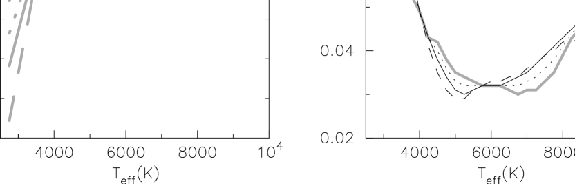
Figure 2: Relationships between stellar effective temperatures and colors relating the 692 nm to the SDSS $r$ filter (left panel) and the 880 nm to the SDSS $z$ filter (right panel). These colors are calculated based on model stellar spectra for ${\rm 3500\leq T_{eff}\leq 10^{4}}$ K at $log(g)$ values of 4.0 (black dashed line), 4.5 (black solid line), and 5.0 (black dotted line). Linear extrapolations from these curves are used to predict the colors for ${\rm T_{eff}<3500}$ K and a curve at ${\rm log(g)=5.5}$ that are not covered by the model spectra. Solar metallicity, ${\rm[Fe/H]=0}$ is used here. The extrapolated curves are shown in grey.

The Dartmouth isochrones already predict absolute $Kp$, $B$, $V$, SDSS $griz$, $J$, and $Ks$ magnitudes, but not magnitudes for the specialized 692nm and 880nm filters used in speckle imaging. To add absolute magnitudes for the 692nm and 880nm filters to the isochrone data, color$-$$T_{\rm eff}$ relationships are derived that relate these magnitudes to SDSS magnitudes. These color$-$$T_{\rm eff}$ relationships are calculated based on solar metallicity model spectra published by Munari et al. (2005), the filter transmission curves, the QE curve of the DSSI CCDs, an atmospheric extinction curve for Mauna Kea at the typical observing airmass of 1.3, and the AB magnitude system. The color$-$$T_{\rm eff}$ relationships between the SDSS magnitudes and speckle imaging filters are shown in Figure 2.

Because the lowest $T_{\rm eff}$ in the model spectra of Munari et al. (2005) was 3500 K, the color$-$$T_{\rm eff}$ relationship is linearly-extrapolated down to 2750 K (although the lowest $T_{\rm eff}$ actually found in the isochrones is $\sim 3000$ K). Additionally, to obtain magnitudes for stars with $log(g)>5$, a $log(g)=5.5$ curve is found by linear extrapolation of the colors predicted at $log(g)=4.5$ and 5.0. These extrapolations are indicated in Figure 2 with light grey lines. For any star defined by $log(g)$ and $T_{\rm eff}$, the absolute magnitudes in the speckle bandpasses can now be found by interpolating between the two bounding curves in the color$-$$T_{\rm eff}$ relationships given their absolute $g$ or $z$ magnitudes. These calculations are done assuming solar metallicity models for each star. Metallicity has a noticeable, but small effect on colors for stars cooler than 4000 K which increases with decreasing effective temperature. At $T_{\rm eff}$$=3000$ K, there are color differences of $\sim 0.02$ in $880-z$ and $\sim 0.15$ in $692-r$ when comparing $\rm[Fe/H]$$=-0.5$ models to solar metallicity models. Thus, there is additional uncertainty in modeling fluxes in the speckle filters among cool stars. This mainly impacts a few of the faint neighbor stars discussed in §6.

5 FALSE POSITIVE PROBABILITY ANALYSIS

A false positive probability is determined for planet candidates orbiting each KOI star that is sufficiently isolated from detectable neighbors such that the KOI star is the only detected star near the source of the candidate signal. This analysis compares the probability of the KOI being a planet host to the probability that a nearly co-aligned and fainter field star is the source of a false positive signal (ie. an eclipsing binary or transiting planet). The scenario of an unresolved triple KOI in which two components form an eclipsing pair is not considered here because for these it is difficult to calculate some of the complex scenarios for a given system. Scenarios such as these have been considered by Fressin et al. (2013) who found that the incidence of false positives attributable to an eclipsing secondary component in a hierarchical triple stellar system are quite low, especially among candidates of Neptune and smaller planets like in the sample considered here.

We estimate the false positive probability for each planet candidate by integrating the parameter space not excluded by Kepler data or follow-up observations with respect to a Galactic model. This method is based on the approach described in Barclay et al. (2013) and Wang et al. (2013, 2014). The information used to restrict the parameter space is the transit depth, the Kepler out-of-transit pixel response function (PRF) centroid statistic and the 692 nm Gemini speckle and any near-IR AO observations of the star. The PRF is the observed appearance of point sources and depends on the PSF produced by the Kepler optics, spacecraft jitter, focus, and spectral class of a given point source (although the latter effect is not considered significant enough to treat individually). The measured PRF and its centroid statistic (Bryson et al., 2013), the quarter-by-quarter standard deviation between a stellar centroid in an out-of-transit image and the difference image between in-transit and out-of-transit light curve points are products of the Kepler pipeline (Tenenbaum et al., 2013, 2014).

The transit depth provides a limit on the faintest star that could produce a false positive signal matching the light curve. This comes from assuming a total eclipse by a background eclipsing binary star of identical components, which would produce a 50% eclipse depth. This maximum eclipse depth is adopted under the expectation that for more general binaries with unequal mass components, the larger star will be brighter in the Kepler bandpass. For a maximum eclipse depth, the background star, outside of eclipse, would be ${\Delta}Kp_{max}$ magnitudes fainter than the KOI and the observed transit depth can be expressed in terms of $\delta$, the KOI’s fractional transit depth: ${\Delta}Kp_{max}=-2.5{\times}log_{10}(2\delta)$. For example, if the observed transit depth were 100 ppm, this could be induced by a eclipsing binary of at most $Kp=9.25$ magnitudes fainter than the KOI. Our estimates of the transit depth are taken from the Kepler data analysis pipeline (Jenkins et al., 2010; Tenenbaum et al., 2013, 2014). Values for ${\Delta}Kp_{max}$ are listed in Table 5.

The Kepler out-of-transit PRF centroid statistic is used to set an exclusion radius for each planet candidate. Any star outside this exclusion radius is excluded from being the source of the candidate transit signal because any such source outside this radius would produce a larger centroid statistic. To find the exclusion radius, we use a $3\sigma$ threshold where $\sigma$ is the PRF statistic discussed above. These exclusion radii establish which KOI stars are sufficiently isolated for the analysis as well as restrict the area inside of which false positives are modeled. Values for the exclusion radius, $r_{ex}$, are listed in Table 5. In the case of KOI 2311, no exclusion radius could be determined due to the lack of PRF centroid data on this star. As discussed in §6, there are 8 candidate planets transiting 5 KOI stars that show a neighboring star within the exclusion radius. These candidates, plus the two of KOI 2311 are excluded from the validation calculation.

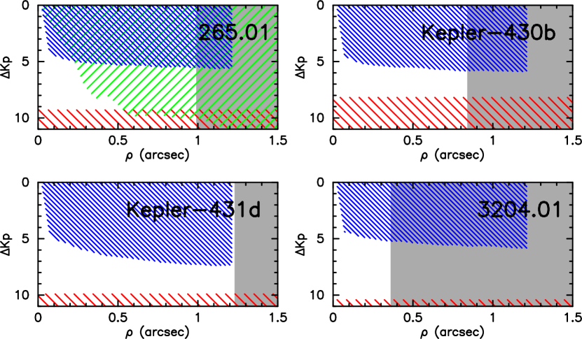
Figure 3: Areas of parameter space where data excludes background stars as the source of a false positive planet signal are shown in terms of the relative Kepler magnitudes fainter (${\Delta}Kp$) and angular separation ($\rho$) with respect to 4 example host stars. Stars are excluded from the blue hashed areas by 692 nm speckle imaging and the green hashed area by $Ks$-band adaptive optics imaging. The red hashed area shows regions below the minimum brightness star (${\Delta}Kp_{max}$) that could produce the observed transit depth. The grey area blocks out areas beyond the exclusion radius set by Kepler PRF centroids statistics. Predictions for the number of background stars that would lie in the remaining white area are used to validate the planets. Labels in each panel indicate the KOI star and planet.

We then include both AO data and DSSI speckle data – we convert the $K$-band AO data to ${\Delta}Kp$ using the equations of Howell et al. (2012) while we utilize the 692 nm DSSI data and assume no difference between this bandpass and $Kp$. This provides a brightness-dependent limit on the maximum separation between a target star and a false positive inducing star. The relative brightnesses and angular separations of potential background stars excluded by the photometry, centroid statistics and transit depths for 4 KOIs are shown in Figure 3.

There are 18 candidate planets orbiting 12 stars that qualified for the validation tests. We use the TRILEGAL galactic simulation (Girardi et al., 2012) to first estimate the stellar population within $1\arcdeg$ around the target star. We then integrate the region of parameter space not excluded by observations with respect to the population model. This provides a number of false positive stars, which is usually much less than 1. We then estimate what fraction of these are likely to be either background eclipsing binaries or background planet hosts (Slawson et al., 2011; Burke et al., 2014). Finally, we compare the number of false positives like this in the entire Kepler data set (i.e. we multiply the number of false positives for this star by the Kepler sample size of 150,000 (Koch et al., 2010) with the predicted number of planets like this in the Kepler data set (Fressin et al., 2013)). The ratio of the total planets to the total number of planets plus false positives yields the probability that a candidate is a planet.

If the planet candidate is in a multi-planet system we boost the odds that the candidate is a planet by a factor of $\sim 30$ for two-candidate systems. This multiplicity boost is justified on the basis of statistics done on the Kepler sample (Lissauer et al., 2012, 2014). Assuming false positives are randomly distributed among targets, multiple planet systems should not have a higher false positive rate than other targets. It is found that a large fraction of KOIs with at least one planet candidate are found to have at least two candidates, meaning a larger fraction of the planets in these systems are real. Table 5 lists the total validation level for each candidate around an isolated star for which PRF centroid data is available. Two of the systems are designated Kepler-430 and Kepler-431 as newly-validated multi-planet host stars hosting a total of 5 planets validated at $\geq 99.8$%. The letter designations for these planets are given in the table.

Several of the planets around these KOIs have previous validation calculations done or have been deemed validated. Xie (2014) showed that the two current planet candidates of KOI 274 exhibited anti-correlated transit timing variations, validating both as interacting planets. Wang et al. (2014) used the native seeing UKIRT $J$-band survey images of the Kepler field to help calculate validation percentages for the multi-planet KOIs 115, 274, 284, 369, 2311 and 3097, including validation boosting due to their planetary multiplicities. For KOI 115.01 they report a 99.8% validation (considering it part of a 3-planet system in contrast to our study that excludes KOI 115.03 due to low detection significance). Wang et al. also reported validation levels above 90% for KOIs 115.02 and 284.01, along with lower levels for the other candidates. Rowe et al. (2014) validated a set of multi-planet KOIs including KOIs 115, 274, 284, and 369 by incorporating various tests on the Kepler data and external data products to arrive at $>99$% validation levels for their hosted planets.

6 NEIGHBORING STARS

6.1 Observed Properties of Neighboring Stars

The neighboring point sources (hereafter assumed to be stars) detected around 7 of the KOIs in the high resolution images as well as native seeing survey images are listed in Table 6. The table provides the relative separations ($\rho$), position angles ($\theta$), and magnitudes fainter than the KOI (${\Delta}$mag). Here, each neighbor star is given a designation of “B” or “C” as an identifier. These stars could be foreground or background stars that are closely aligned by mere chance with the KOI star or may be gravitationally bound secondaries. The closer and brighter these neighboring stars are, the more likely they are to be gravitationally bound to the KOI, as discussed below.

Table 6 shows that 7 KOI stars have a neighbor $\leq 4\arcsec$ away detected in high resolution images. In the case of 5 of these KOIs, one neighbor lies within the exclusion radius for all planet candidates (KOI 268B, 284B, 1964B, 3255B, and 3284B). Such neighbors are potential sources of a false positive (ie. an eclipsing or transiting system that is blended with the KOI). Even very faint neighbors, with magnitudes relative to the KOI star of ${\Delta}Kp=9-10$ can produce a transit-like signal at the level expected for an Earth-sized planet transiting a Sun-like star (Morton & Johnson, 2011).

The more distant neighbors should not be considered possible sources of a false positive. These stars are nonetheless important to consider as possible members in a stellar binary with the KOI and for their dilution of the KOI light curves. To correct for dilution, a search was made for any star that could possibly dilute the light curve at a 1% level or greater. Both the high resolution images and other ground-based imaging surveys such as the UKIRT $J$-band survey and a catalog of $UBV$ photometry by Everett et al. (2012) were used. Some neighbors are left out of this search, namely any listed in the KIC, because any excess flux blended into the light curve by KIC stars will have already been estimated and removed by the Kepler pipeline. Two significant KIC stars were noted near the KOIs in this sample: KIC 11560901, about $8.5\arcsec$ away from KOI 2365 (Kepler-430), and KIC 8212005, about $12.9\arcsec$ away from KOI 2593.

6.2 Previous High Resolution Imaging

Several of these stars have been previously observed with high-resolution imaging by Adams et al. (2012, 2013), Law et al. (2014) and Lillo-Box et al. (2014). KOI 1537 was reported by Adams et al. (2013) to have a close neighbor with a separation of $0.13\arcsec$ in $Ks$ AO images. The same KOI was observed by Law et al. (2014) in an optical AO (RoboAO) survey of KOIs, but no neighbor was found. Their non-detection would be consistent with the close separation and RoboAO imaging resolution. No neighbor of KOI 1537 is detected in our speckle data. This is surprising given the high spatial resolution, which would easily resolve the separation, and the small magnitude difference ${\Delta}Ks=0.15$ reported by Adams et al. (2013). The limiting contrast for detecting neighbors at a separation of $0.13\arcsec$ in the 692 nm and 880 nm images is 5.37 and 4.69 magnitudes respectively. These apparently discrepant observations cannot be attributed to a hypothetical very red neighbor. The color $880-Ks=1.08$ is found for KOI 1537 from its isochrone fit, meaning any line-of-sight neighbor would need to be at least as red as $880-Ks\simeq 5.6$, or redder than the reddest stars ($880-Ks=3.9$) found in the isochrones of §4.3. In light of this observation, KOI 1537 is treated as a single star here. Adams et al. (2012) observed KOIs 268 and 284 and detected the neighbors of both stars with $J$ and $K$ magnitude differences in agreement with the values published here. (Note that the position angles they reported for KOI 268 are apparently erroneously flipped.) KOI 115 was observed by both Law et al. and Lillo-Box et al. It was seen as single by Law et al., in agreement with our data. Lillo-Box et al., who observed with a larger field-of-view, reported a neighbor to KOI 115 about $4\arcsec$ away and 8 magnitudes fainter in $i$. Law et al. and Lillo-Box et al. also observed KOI 2593. Both reported it as a single source. In addition to KOIs 115, 1537 and 2593, three other stars (KOIs 268, 1964, and 2365) were observed by Law et al. in the optical and, in the case of KOI 1964, in a near-IR $Ks$ image. They reported the closest neighbor to KOI 268 to have an optical magnitude difference of $3.82\pm 0.27$, which is consistent with our near-IR magnitude differences for a neighbor redder than the KOI. Their $Ks$ observations of KOI 1964 were in good agreement with ours. They found KOI 2365 (Kepler-430) to be single, again in agreement with our results.

6.3 Distinguishing Bound Companions from Field Stars

Various evidence may be used to determine if neighboring stars are gravitationally-bound secondaries or unrelated, line-of-sight field stars. A full simulation of the properties and frequency of secondary stars and field stars could be used. Instead, in this study, a series of simpler tests are applied. These tests consider the brightness of the neighbor, its angular separation from the KOI star, and the stellar colors for those stars observed at multiple wavelengths. Other approaches to using multi-color photometry to investigate the possible physical association of neighbor stars with KOI stars may be found in Gilliland et al. (2014) and Lillo-Box et al. (2014).

6.3.1 Angular Separation and Apparent Brightness

First, the angular separation from the KOI star and magnitude of the neighbors are examined relative to a random distribution of field stars at the location of the KOI. In doing so, an initial assumption is made that KOI stars are not preferentially co-aligned with unrelated field stars. A randomly-generated set of stars representing a 1 square degree field is produced at the location of the KOI using the TRILEGAL Galaxy model (Girardi et al., 2005) Version 1.6 web form. The model predicts apparent magnitudes in various passbands including $J$ and $Ks$. The number of stars in the TRILEGAL model brighter than the neighbor star is found and multiplied by the ratio of the circular area inside the neighbor’s separation ($\rho$) to the 1 square degree model field to get a “background” probability, $P_{BG}$. $P_{BG}$ is the likelihood that a field star of the same brightness or brighter than the neighbor would lie by chance at the same or a smaller angular separation from the KOI. In most cases the $Ks$ bandpass is used for this calculation because it yields the lowest probabilities. To find approximate $Ks$ magnitudes for the neighbors, the differential photometry of the AO images is used along with the $Ks$ magnitude of the associated 2MASS point source (Skrutskie et al., 2006). For neighbor “C” of KOI 3284, the $J$ magnitude of the UKIRT survey was used instead due to unavailable $K$-band data. The background probabilities along with the apparent $Ks$ magnitudes derived for each source are listed in Table 7. As an empirical check on this method, the calculation was also run using Kepler magnitudes of sources extracted from 1 square degree of the KIC at the location of each KOI. The probabilities determined from the KIC agreed with those of the TRILEGAL model to within a factor of 2 (some were higher, others lower).

Note that in many cases $P_{BG}$ is quite low, a promising indication that the neighboring stars are gravitationally-bound companions. The expectation is that gravitationally-bound secondaries outnumber co-aligned neighbors in high resolution images such as these, especially within separations of $\sim 1.2\arcsec$ (Horch et al., 2014). For this reason, these close neighbors are likely dominated by bound companions. However, false positive scenarios for small planet candidate KOIs include the case of large planets transiting background (or field) stars that are closely co-aligned with the KOIs. These cases can appear much like the observed double KOI sources we have detected in terms of relative magnitude and separation (Fressin et al., 2013). For these cases, the assumption that background stars are randomly-distributed in the sky is invalid and the low values of $P_{BG}$ are best treated as just one of several indicators that help distinguish between field stars and bound companions. These probabilities are most applicable for neighbor stars that lie outside the exclusion radius. On the other hand, a low value of $P_{BG}$ for a neighbor star inside the exclusion radius can be explained as either a bound companion or a false positive.

6.3.2 Colors and Relative Brightness of Neighbors

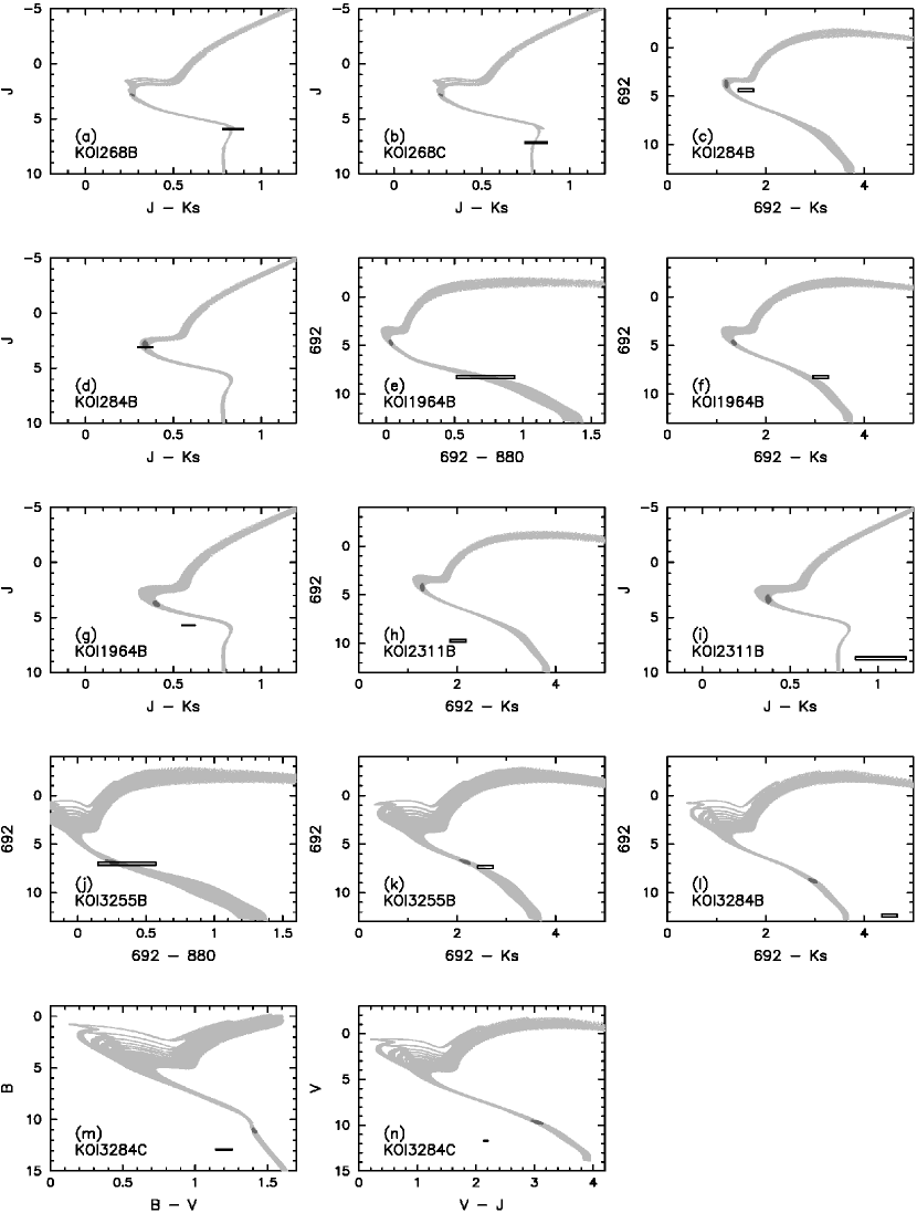
Figure 4: A comparison of the relative magnitudes and colors for 6 KOI stars with close neighbors. The absolute magnitudes and colors of each KOI star are predicted on the basis of fitting its stellar properties (Table 4) to Dartmouth isochrones. The $1\sigma$ confidence intervals are indicated by the dark grey regions in each plot. The set of isochrones that pass through this set of properties are shown in light grey and represent the predicted absolute magnitudes and colors for any secondary stars. The photometry of each neighbor star relative to the KOI star is used to place it on the same plot. The location of the neighbor stars are shown as rectangular boxes that outline the bounds of the $1\sigma$ uncertainties in the relative photometry. The location of the neighbor relative to the isochrones is one indicator that helps distinguish unassociated field stars from gravitationally-bound companions.

Both stars of gravitationally-bound pairs should lie on the same isochrone and this can be tested for KOIs that have been observed at multiple wavelengths. The test relies on the relative brightnesses and colors of the two stars. To determine these, the isochrone fits are used to find the colors of the KOI stars while the differential photometry of the imaging provides relative colors and brightnesses of the neighbor. Table 8 lists the relative brightnesses and colors for the double KOI sources that have been observed in more than one filter. The magnitudes in the table are absolute magnitudes for the KOI stars and likewise for their neighbor stars if they are gravitationally bound. Figure 4 compares the magnitudes and colors of 6 KOI stars and their close neighbors alongside the isochrones describing the KOI star properties. The colors and magnitudes of each KOI star (within its $1\sigma$ uncertainty range) are indicated by dark grey regions in each panel. The light grey regions show the set of isochrones that pass through these ranges of uncertainty. The magnitudes in each plot represent absolute magnitude as predicted by the Dartmouth isochrones or, in the case of the 692 nm and 880 nm filters, calculated from the isochrones’ SDSS magnitudes as described in § 4.4. The relative magnitude and colors of the neighbors with respect to the KOI stars are calculated using the relative photometry provided by the speckle imaging analysis and near-IR AO images. The neighboring stars’ colors and magnitudes are shown as rectangular boxes that indicate the $1\sigma$ photometric uncertainties.

In most panels of Figure 4 the relative colors and brightnesses of the close neighbor stars are consistent with the isochrones describing the KOI stars. In other words, most of the neighbors are consistent with being gravitationally-bound secondaries. However, in five panels ($g$, $h$, $l$, $m$ and $n$) the neighbor falls quite far from the isochrones as would be expected in the case of most field stars. The neighbors of KOI 1964 (panel $g$) and KOI 2311 (panel $h$) are fainter and/or bluer in these colors than main sequence stars at the distance of the KOI, but this situation is not seen in other plots for the same KOIs (panels $e$, $f$ and $i$). Neighbor C to KOI 3284 is too faint or blue relative to the Main Sequence in both colors examined. In the case of neighbor B to KOI 3284 (panel $l$), the neighbor is too red relative to the Main Sequence. It is also too faint to be a Milky Way giant. In this case, the neighbor is so red and faint relative to KOI 3284 (itself a M dwarf) that, if a bound companion, its luminosity would place it at an extremely low mass where the model colors are most uncertain. This case should be treated with some caution.

6.3.3 Color Relative to Background Population

To compare the colors of the close neighbors of 6 KOI stars to the colors of field stars of the same apparent brightness, the TRILEGAL Galaxy models are used again (the same 1 square degree field populations used in §6.3.1). This time the field star populations are restricted to those stars within one magnitude of the apparent magnitude of the neighbor star in the bluer of two filters being considered. The number of field stars is plotted as a function of colors in Figure 5. The colors of the neighboring stars are indicated by vertical lines (solid lines represent the central value and dotted lines the $1\sigma$ uncertainty interval).

The color distributions of the field stars show several features. In $J-Ks$, the peak near 0.25 is due to large numbers of upper main sequence plus turn-off stars, a second peak near 0.6 is due to giants, and some plots show a peak at 0.75 due to lower main sequence dwarfs. The same features are seen in $692-Ks$ at 1.1, 1.8, and 2.25 respectively. The upper Main Sequence plus turn-off stars and giants show up as peaks near 0 and 0.15 respectively in $692-880$. The red tails of the $692-880$ and $692-Ks$ colors are comprised of the lowest mass dwarfs.

The field star color distributions are affected by reddening while the colors derived for the secondary stars are intrinsic colors (zero reddening effects). However, extinction is quite small in the TRILEGAL models where $A_{V}=0.03-0.04$ to distant lines of sight in the Kepler field and so reddening corrections in the $692-Ks$ color would be only $0.02-0.03$ magnitudes using the extinction curve of Cardelli et al. (1989). For this reason, no adjustment for the effects of reddening has been made.

In each panel of Figure 5, the colors of the neighbor stars are either consistent with the bulk of the field star distribution or redder than it. Assuming field stars are distributed randomly on the sky around each KOI, a first order expectation is that their colors will be drawn from this same distribution. For this reason, the relatively red colors of the neighbors seen in panels $e$, $f$, $i$, $k$ and $l$ (ie. KOI 1964B, 2311B, 3255B and 3284B) are best explained by low-mass gravitationally-bound secondaries (although the extreme color measured for KOI 3284B was difficult to explain as discussed earlier). Two other neighbor stars, KOI 268 B and C (panels $a$ and $b$) are also quite red, but so too are more field stars in $J-Ks$.

6.3.4 Assessing the Nature of Each Neighbor Star

None of the observations definitively distinguishes between gravitationally-bound or field star neighbors, but in most cases the evidence points toward the close neighbor being a gravitationally-bound secondary. Values of $P_{BG}$ are quite small for all but the three most distant neighbors (KOI 3255C, KOI 3284C and KOI 4407C), which means these have a reasonable likelihood of being nearby field stars. KOI 1964B and KOI 2311B also show some evidence of being field stars based on some colors ($J-Ks$ in the case of KOI 1964B and $692-Ks$ in the case of KOI 2311B). However, KOI 1964B is less conclusive because in the other colors examined it appears to be a relatively low-mass, red, bound companion. The photometry for KOI 3284C is inconsistent with that of a binary companion, but is internally consistent with that of a background dwarf (see § 6.4.2).

The other 5 neighbors with multi-band photometry (KOIs 268B, 268C, 284B, 3255B and 3284B) are the most consistent with being bound companions. KOI3255C has photometry in $J$ only and KOI 4407B and C in $Ks$ only, so their natures remain indeterminate.

Overall, among the 11 neighbor stars in this study 8 have multi-band photometry. Of those 8, five are deemed likely bound companions, one a likely field star, and the two others remain too ambiguous to classify. Based on this, the fraction of likely bound companions may be as high as 87.5% or as low as 62.5%. This can be compared to the lucky imaging survey of 174 candidate or confirmed KOI host stars by Lillo-Box et al. (2014). Among their targets observed in both $i$ and $z$ filters, five were found with close companions, but they considered only one of them to be a bound companion. The significance of the lower fraction of bound companions is difficult to quantify, but given the larger mean separations for the companions in the Lillo-Box et al. survey, a greater fraction of field stars is reasonable. In a study of 23 KOIs observed in two filters with HST/WFC3, Gilliland et al. (2014) quantified the odds for neighboring stars to be the bound companions of KOIs. They found 8 neighboring stars were physically associated with the target KOI, and 6 of these had relatively close separations of $<1\arcsec$. Clearly, high resolution imaging inside of $\sim 1\arcsec$ is needed to find most of the wide binary companions to KOIs.

6.4 Blending Corrections for Crowded KOIs

In order to correct the light curves for the effects of blending, neighbors’ stellar properties must be estimated. Two separate scenarios are considered for the status of these neighbor stars: bound companions and unrelated field stars. For completeness, and because most of the neighbor stars are consistent with being gravitationally-bound secondaries, a calculation is made for each neighbor assuming it is gravitationally bound. In the case of binaries, the secondary star properties are more easily constrained by the observations because each component shares a common distance, extinction, composition and age. The second case, that of neighbor stars being unrelated field stars, is considered for a few cases where evidence suggests or allows this scenario. Constraining the properties of field stars can prove more difficult. To find the stellar properties of assumed secondary stars, the relative photometry is used for isochrone fits as described in § 6.4.1. To find properties of field star neighbors, the most likely types of stars are identified in Galaxy models as discussed in § 6.4.2. For either case, an aperture correction is found for each star in § 6.4.3. Finally, a blending correction, is formulated in § 6.4.4 based on the $Kp$ magnitudes and aperture corrections for each star in the blend. These corrections are used to reevaluate the planet properties for crowded KOIs as described in § 7.

6.4.1 Properties Assuming Neighbors are Secondary Stars

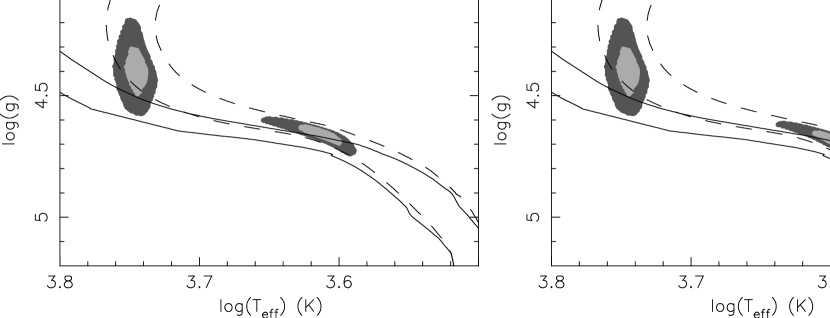
Figure 6: Results of isochrone fits for the double source KOI 1964 (an assumed binary star). $T_{\rm eff}$, $log(g)$ and $\rm[Fe/H]$ for the brighter KOI star (primary) are fitted to a set of Dartmouth isochrones. The probable ranges on $log(g)$ and log($T_{\rm eff}$) for the primary are shown in the shaded region in the upper left of each panel, centered near ${\rm log(T_{eff})=3.74}$ and ${\rm log(g)=4.39}$. The light grey color indicates the $1\sigma$ range in stellar properties while the darker grey corresponds to the range $1-2\sigma$. The same fit also produces a best value and range for $M_{\star}$, $L_{\star}$, $R_{\star}$ and absolute magnitudes in various filters. A neighboring star is found (secondary) and its properties are found separately in 4 filters (each shown in one of the 4 panels as labeled by filter). The data in each filter consists of a magnitude difference that maps the primary star properties to a range in secondary properties along the isochrones. The properties of the secondary are shown near ${\rm log(T_{eff})=3.59}$ and ${\rm log(g)=4.70}$ using the same greyscale representation. The full range of isochrones are shown as lines in each panel with dashed lines for 13 Gyr isochrones and solid lines for 1 Gyr isochrones. The upper lines, dashed or solid, represent ${\rm[Fe/H]=+0.4}$ and the lower lines represent ${\rm[Fe/H]=-0.40}$. See §4.3 for details.

Each image taken in a different filter provides an independent measurement of the relative brightnesses of the secondary and primary stars. The magnitude differences, along with their observational uncertainties, map the probability distribution of the primary star properties along a set of isochrones into a distribution of secondary star properties. Figure 6 shows the distribution of primary and secondary star properties in $log(g)$ and $T_{\rm eff}$ for the double source KOI 1964 observed in four different filters. Curves outline the range of isochrones used in the model fits.

When relative magnitudes are available in multiple filters, the secondary properties derived from each are combined in a weighted average to obtain a final estimate. One of the most important secondary properties is $Kp$ because it helps to determine the excess flux contributed to the light curve by the secondary. Table 7 lists both apparent and absolute $Kp$ magnitude from the isochrone fits for each multiple KOI (apparent $Kp$ are mean values calculated from multiple filters and the absolute $Kp$ values are individual values for each filter). Kepler magnitudes are reported in the KIC for each of the blended KOIs considered here. In cases where neighbors lie $\leq 1.5\arcsec$ from the KOI, the KIC magnitude is assumed to be the blend of each component whereas more distant neighbors are assumed to not contribute to the cataloged magnitude of the KOI. Table 7 also contains the number of standard deviations each individual filter’s results are from the mean $Kp$. These numbers indicate how well data from different passbands match expectations for a bound companion. The photometry of both neighbors to KOI 268 and the neighbors of KOIs 284 and 3255 agree well with expectations for bound secondaries. The photometry for the neighbor of KOI 1964 agrees less well, but is plausibly consistent with a bound companion. The photometry for the neighbors of KOI 3284 and KOI 2311 is inconsistent with a bound companion. This result is similar to the previous analysis indicating these neighbors are likely to be field stars. Table 9 gives the averaged values of ${\Delta}Kp$ for each KOI and neighbor based on the individual photometric measurements of each system. This table lists separate values for different planets in multi-candidate systems since the blending situation will later be considered separately for each planet.

6.4.2 Properties Assuming Neighbors are Field Stars

As discussed in § 6.3, there are three neighboring stars with multi-color photometry that show colors plausibly inconsistent with those of a gravitationally-bound companion (KOI 1964B by its $J-Ks$ color, 2311B by its $692-Ks$ color and 3284C in all colors). To determine what types of field stars match the observed brightness and colors, the TRILEGAL Galaxy models are used once again. This time the area covered by the Galaxy models is increased to 4 square degrees for KOI 1964 and 10 square degrees for KOI 2311 to ensure a rich sample of model stars. The subset of model stars whose apparent magnitudes lie within 1 magnitude of the neighbor star and whose colors fall within the observed uncertainty intervals listed in Table 8 are extracted. Here, the apparent magnitude adopted is that of the bluer filter and each subset contains $\sim 200$ stars or more. The field stars are comprised of either dwarfs, evolved stars or both in various cases. For KOI 1964B, evolved stars (with $log(g)$$<4.0$) are dominant with dwarfs comprising just 13 out of the 284 total model stars (4.6%). For KOI 2311B the situation is much different with dwarfs accounting for 11771 out of 11825 model stars (99.5%) and for KOI 3284C the model contained no evolved stars among the 264 stars matching $B-V$ or the 195 stars matching in $V-J$.

A similar analysis is done on the three neighbor stars with photometry available in only one filter. For these stars, KOI 3255C and KOI 4407B and C, the subset of stars drawn from the TRILEGAL model is unconstrained by color and representative of all field stars matching the brightness of the neighbor. For KOI 3255C, potential background stars are almost entirely dwarfs (32158 out of 32724 stars or 98.3%). Evolved stars are more likely as background cases for KOI 4407B (only 620 out of 1786 or 34.7% are dwarfs) and for KOI 4407C (12363 out of 14706 or 84.1% are dwarfs).

While the stellar properties of the potential background stars can vary greatly (e.g., different luminosity classes or stellar radii), the most important property to examine is the relative Kepler magnitude, which determines the amount of blending. ${\Delta}Kp$ is largely a function of effective temperatures and the TRILEGAL stars of all luminosity classes are combined for its determination. For cases where a presumed field star fell within the exclusion radius (field stars that could be false positive sources), a careful consideration of its other stellar parameters would be needed, but this situation was not encountered in our sample.

Figure 7 shows the distributions in ${\Delta}Kp$ for the 6 potential background neighbors and Table 10 gives the mean differences in Kepler magnitude for each case. Note that the table lists the status of two neighbors as bound companions (KOI 3255B and KOI 3284B) and for these the Kepler magnitudes are the same as in Table 9. It is the second neighbors (C) of these KOIs that are treated as field stars. Figure 7 shows the obvious differences in the distributions of possible ${\Delta}Kp$ values between those stars with color information and those without it. With constraints on the color, the uncertainty on ${\Delta}Kp$ is as low as $0.05-0.10$ magnitudes. This is true even for KOI 1964B where the color comes from near-IR measurements. For those neighbors observed in only one filter, the uncertainty in ${\Delta}Kp$ is at least 2 magnitudes. This uncertainty is partly due to the near-IR wavelengths of these observations; a single photometric measurement in the 692 nm filter, for example, would yield an uncertainty in ${\Delta}Kp$ of $\sim 0.2$ magnitudes due to its closer match with the Kepler bandpass.

6.4.3 Aperture Corrections

The fraction of each star’s flux that falls in the light curve aperture is determined using the Kepler Mission data analysis tools of PyKE (Still & Barclay, 2012), slightly modified for these purposes. The set of pixels in Kepler’s pixel light curve files is analyzed at epochs coinciding with transits calculated from each candidate’s ephemeris. The average of the effects over all epochs should represent the effects of blending in the folded light curves analyzed for planet properties. For KOIs with orbital periods longer than 15 days, each transit time is examined. For shorter orbital periods, fewer transit times are examined for purposes of efficiency (e.g., every 2nd or 3rd transit). Kepler targets shift pixel location with time, however the most significant differences occur between different Kepler quarters as the spacecraft rolls by $90\arcdeg$ and new light curve apertures are used on different CCDs. Because the KOI stars are the brightest star in each aperture, and sampled both in the core and the wings, the PyKE tool kepprf is used to fit its PRF to the Kepler data and report back a source center and the fraction of the flux that falls inside the aperture. For secondary stars, pixel coordinates are fixed relative to the KOI based on the ground-based astrometry. The percentage of the pixel response function of each secondary that falls inside the aperture is determined and reported in Tables 9 and 10. Where these numbers are reported for multiple planet candidates of the same KOI, the quite small differences in flux may be seen.

6.4.4 Corrections for Blended Light Curves

A blending correction must be made to properly interpret the light curves of blended KOIs and revise the planet properties derived from them. Furthermore, because for some blended KOIs, more than one star could be the source of the transit-like variations (ie. be the host star), the effects of blending are considered with respect to each star. The goal is to describe an intrinsic light curve for each possible host star.

The amount of dilution in these light curves and its effect on a key Kepler measurement, the intrinsic fractional depth of a transit signal, $\delta_{true}$, may be written as:

$$\delta_{true,i}=\delta_{obs}\left(1+\frac{1}{F_{i}}\sum_{\stackrel{{\scriptstyle j=1}}{{j\neq i}}}^{N}F_{j}\right).$$ (1)

Here, the transit (or eclipse) is assumed to occur to the $i$th star, and the observed fractional transit depth is $\delta_{obs}$. The intrinsic fractional transit depth of the $i$th star, $\delta_{true,i}$ is found from $\delta_{obs}$ using a blending correction factor dependent on the flux of all stars in the blend. Similar treatments were adopted by Law et al. (2014) and Lillo-Box et al. (2014).

Tables 9 and 10 list the blend corrections calculated from Eq. 1 ($\delta_{true}/\delta_{obs}$) using the $Kp$ magnitude for each component converted to relative flux and with the fluxes modified by the aperture corrections of § 6.4.3. It should be noted that of course these blend corrections are based on the mean predicted values of ${\Delta}Kp$ and are subject to its uncertainties which, for cases of field star neighbors observed in a single filter, can be quite large.

7 PLANET PROPERTIES

Revised planet properties are derived based on the new stellar properties and corrections for blending in the light curves of crowded KOIs. All of the KOIs have “best” current values for various stellar and planetary properties, which can be found in the Cumulative KOI database at the NASA Exoplanet Archive or the stellar properties catalog of Huber et al. (2014), which includes the stellar masses.

A first order revised planet radius may be found by scaling the current value of the planet radius by a factor equal to the ratio of the new stellar radius to the current stellar radius (one used by the mission for its current light curve fit). Such a scaling is ideal for cases where the revisions to stellar radius are small, although here it is applied to all cases for illustrative purposes. For KOIs with close secondaries, multiple scenarios are considered wherein the transiting body may orbit the secondary. In this case, “close” secondaries are only those stars falling inside the exclusion radius around each KOI (so could be the planet host; see §5). Table 11 lists the isochrone fit values for stellar radii, masses and effective temperatures for each KOI star as discussed in §4. In this table, the same properties listed for the neighbor stars represent those derived from isochrone fits under the assumption that the neighbors are gravitationally bound as described in (§ 6.4.1). Also listed are transit (ie. planet orbital) periods, $P_{p}$, and the planet-to-star radius ratio, $R_{p}/R_{\star}$, a parameter found from light curve fits and taken from the cumulative KOI database. This radius ratio, when multiplied by the new stellar radius, scales the planet radius in accordance with the revised stellar radius. The other scaling done to the planet radii accounts for the blends; here, the value $\sqrt{\delta_{true}/\delta_{obs}}$, derived from Equation 1 (see Tables 9 and 10), is found and applied as a multiplicative factor that increases planet radii. Two (generally) different values of the revised planet radii are given in Table 11 representing the case where each neighbor is assumed to be a binary companion star ($R_{p{\rm BIN}}$) and the case where at least one neighbor is assumed to be a background star ($R_{p{\rm BG}}$) as listed in Table 10. Cases where the KOI arises due to transits of an object orbiting a neighboring field star are not examined because such situations are complicated by large uncertainties in determining the Kepler magnitude of some neighbors and the often wide, bimodal distributions in background star radii (ie. they may be either dwarfs or evolved stars). Note too that a complete reevaluation of the planet radii could be performed from new light curve fits, but such reanalysis lies beyond the scope of this study.

The magnitude of the “deblending” factor varies by KOI. Consider, first of all, the KOI star as the host. For KOI 2311, the secondary is relatively faint so its effects on the planetary radii are negligible. In KOIs 268, 1964, and 4407, estimates for new planet radii are $1-5$% higher after deblending. For KOI 3284, the radius is 8% higher and for KOIs 284 and 3255, the planet radii need adjustment upwards by about 30%. In cases where a secondary star is the potential host star (making the KOI a false positive under our definition), the effects on planet radius can be even larger and perhaps be large enough to rule it out as a planet. This can be seen in a comparison between the derived radius of the same planet assuming the KOI as the host star versus the secondary star as the host. In the case of KOI 268.01, the radius is 3 times larger if it orbits the secondary (it is a giant planet rather than sub-Neptune size). For KOI 2311.01 and 2311.02, planet sizes change from Earth-like to more like that of Neptune. Finally, it is notable that in none of the cases would a candidate orbiting one of these secondary stars require a radius exceeding that of a giant planet (ie. require a stellar eclipse). These examples make it clear that understanding the role of light curve blends alongside uncertainties in stellar properties is vital for understanding the Kepler planet sample.

New stellar masses and effective temperatures invite a recalculation of planet equilibrium temperatures, an indicator of planet habitability. Various assumptions are made in the calculation: circular orbits and planets with an albedo of 0.3 and uniform surface temperature. The planet transit (ie. orbital) periods, $P_{P}$ are used to find the semi-major axis, $a$, of each orbit (given the stellar mass) and this establishes the equilibrium temperatures, $T_{eq}$, listed in Table 11. Examination of the equilibrium temperatures reveals the low-$T_{eq}$ candidates selected for this study. It also shows that lower values of $T_{eq}$ are expected for planets orbiting the potential secondaries as opposed to the KOI stars.

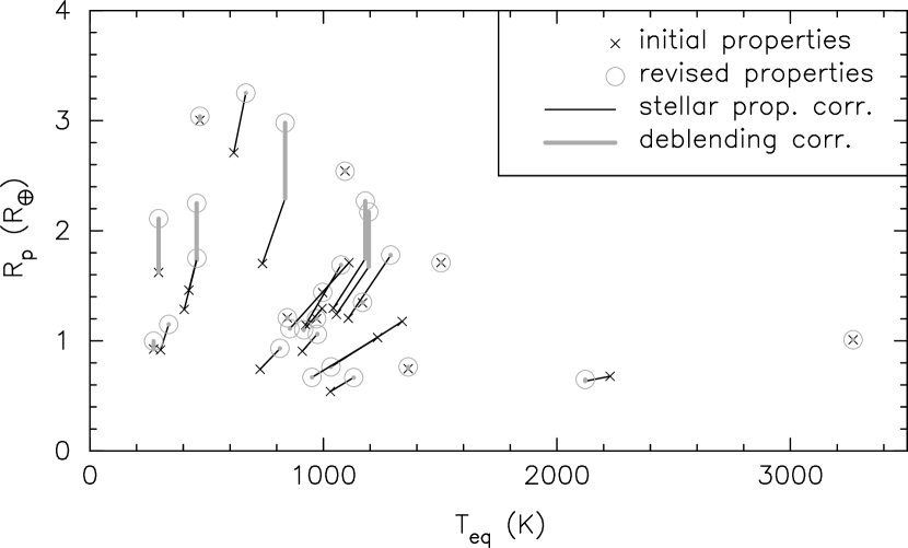
Figure 8: Changes to planet radii ($R_{p}$) and equilibrium temperatures ($T_{eq}$) made as part of this study. Here, each planet or candidate planet is assumed to orbit the KOI star (the brightest star, not any blended neighbor). Initial planet properties are shown with lines connecting them to their revised properties (when applicable) with the corrections due to revised stellar properties shown separately from those due to deblending. Symbols used are defined in the inset box.

Initial and revised planet radii and equilibrium temperatures are plotted in Figure 8. In this case, each planet is assumed to orbit the KOI star. Corrections for the revised stellar properties and those for deblending are shown separately. For this plot, “initial” stellar properties are adopted from the catalog of Huber et al. (2014), in the case of those stars with KPNO 4m spectra taken as part of this study, or are the literature values cited in Table 4 otherwise. The plot shows the considerable corrections due for some KOIs. Mostly, the corrections for stellar properties have resulted in hotter and larger candidates. Deblending corrections increase planetary size estimates.

8 INDIVIDUAL KOIs

An overview of new findings for individual planet candidates and validated or confirmed planets is summarized here. A complete list of the host star properties, neighboring stars not listed in the KIC and planet properties may be found in Tables 4, 6 and 11 respectively.

KOI 115 (Kepler-105):

Two previously-validated planets orbit this isolated solar-type star with orbital periods of 5.412 and 7.126 days. These planets are validated in our study as well and given new radii estimates of 2.54 and 1.44 $R_{\bigoplus}$ respectively.

KOI 265:

This isolated, perhaps slightly-evolved, solar-type star hosts a single 1.71 $R_{\bigoplus}$ planet candidate with a 3.568-day orbital period. We present new $J$ and $Ks$ AO imaging in addition to the speckle imaging for this star to yield a 94% validation level.

KOI 268:

This is a 6343 K dwarf star hosting a single planet candidate in a 110-day orbit. New $J$ and $K^{\prime}$ AO imaging reveals two neighboring stars (B and C) several magnitudes fainter. Since neighbor B lies within the exclusion radius, this planet cannot be validated using our methods. The proximity and relative magnitudes in two filters provide evidence that both of these neighbors are bound companions, but this is less certain than for other KOIs in our study. This KOI is subject to slight blending by its neighbors. If the candidate orbits the KOI star it is estimated to have a radius of 3.04 $R_{\bigoplus}$. If, on the other hand, it orbits the assumed 4007 K dwarf secondary star (neighbor B), the radius would be 9.33 $R_{\bigoplus}$ and its equilibrium temperature would be rather low (217 K).

KOI 274 (Kepler-128):

Two previously-validated planets orbit this slightly-evolved isolated solar-type star with 15 and 22.8-day orbital periods. We validate the planets again with speckle imaging (finding the host star to be single). Both planets have radii near 1.2 $R_{\bigoplus}$.

KOI 284 (Kepler-132):

There is a system of three previously-validated planets and one planet candidate orbiting this solar type star, whose stellar properties we characterize with new spectroscopy. The Kepler light curve is significantly blended by flux from a neighboring star, which falls within the exclusion radius for each planet (so re-validation of this KOI is not attempted here). In addition to speckle imaging, we publish new $J$ and $Ks$ AO photometry here. It is difficult to use the multi-band photometry to determine if the neighbor is a bound companion or field star. Its close angular proximity to the KOI and photometry consistent with that of a bound companion argue that this is the most likely case. If a bound companion star, the planets and candidate planet radii all fall within a $2-3R_{\bigoplus}$ range and have virtually identical radius estimates whether they orbit the KOI or secondary star.

KOI 369 (Kepler-144):

This 6157 K dwarf harbors two previously-validated planets. We provide new spectroscopic characterization and $J$-band AO imaging for this star. No neighboring stars are found, enabling us to re-validate the planets based on the speckle and AO imaging. Kepler-144b and c are found to have radii of 1.78 and 1.69 $R_{\bigoplus}$ respectively.

KOI 1537:

One candidate planet orbits this 6260 K dwarf with a period of 10 days. The speckle imaging presented here shows no neighboring stars for this KOI in contrast to published AO observations in $Ks$ (Adams et al., 2013). The two photometric studies are apparently irreconcilable assuming a very red star. Validation is attempted for this candidate, but the resulting level is fairly low (86.7%). No blending correction is performed for this KOI, resulting in a planet radius of 1.35 $R_{\bigoplus}$.

KOI 1964:

This 5547 K dwarf is observed with both speckle imaging and $J$ and $Ks$ AO imaging. A neighboring star lies about $0.4\arcsec$ to the north and within the exclusion radius of its single 2.2-day orbital period planet candidate. Relative photometry of the neighboring star results in some ambiguity: near-IR colors suggest the neighbor is a background field star while the optical colors are more consistent with those of a bound companion. Both cases are examined and the slight blending effects are evaluated and corrected to conclude that the candidate has a nominal radius of $0.764$ or $0.785R_{\bigoplus}$ if it orbits the KOI star (the two cases represent different blending corrections assuming the neighbor is alternatively a bound companion or field star). If it orbits the neighbor and that star is a 3892 K dwarf secondary, the planetary radius would need to be increased to 2.03 $R_{\bigoplus}$.

KOI 2311:

This solar type dwarf hosts two candidate planets with orbital periods of approximately 192 and 14 days. A new spectral characterization is presented for this star. New optical speckle and AO imaging in $J$ and $K^{\prime}$ reveal a faint neighboring star about $1\arcsec$ away. Since the Kepler data pipeline did not report the astrometry needed to define an exclusion radius, the neighbor is also assumed to be the potential host star. Since the multi-band photometry is ambiguous in terms of determining if the neighbor star is a bound companion or not, both scenarios are examined. The neighbor is relatively faint, so while a deblending calculation is performed, it has no significant impact on interpreting the light curve. The inner planet candidate is found to be 0.932 $R_{\bigoplus}$ if it orbits the KOI and 4.16 $R_{\bigoplus}$ if it orbits the neighbor (here assuming the bound companion scenario). The outer planet candidate is cool (337 K) and small (1.15 $R_{\bigoplus}$) if it orbits the KOI and if it orbits the neighboring star (again assuming a bound companion), it is cold (117 K) and larger than Neptune (5.14 $R_{\bigoplus}$).

KOI 2365 (Kepler-430):

This is a solar type dwarf that hosts two planets and is found to be an isolated star in the speckle imaging and characterized with a new spectrum. Both planets are newly-validated at the 99.9% level using the speckle data and a planet multiplicity boost. The inner planet, Kepler-430b, orbits with a 36-day period and is found to be 3.25 $R_{\bigoplus}$ with $T_{eq}=667$ K. The outer planet, Kepler-430c, orbits in a 111-day period orbit and is found to be 1.75 $R_{\bigoplus}$ with $T_{eq}=458$ K.

KOI 2593:

This is an isolated star hosting a single candidate. New spectroscopy is presented and shows the KOI to be a 6119 K dwarf. The planet is validated at a 90.6% level using speckle imaging along with a $K^{\prime}$ AO image and the planet candidate is found to have a $1.10~{}R_{\bigoplus}$ radius with an equilibrium temperature of 915 K.

KOI 2755:

This is an isolated star hosting a single candidate. New spectroscopy is presented that shows the KOI to be a 5792 K dwarf. The planet is validated at a 82.7% level using speckle imaging and the planetary properties are found to be $R_{p}=1.06R_{\bigoplus}$ and $T_{eq}=974$ K.

KOI 3097 (Kepler-431):

This is a solar type dwarf that hosts three planets. A new spectrum is used to characterize the star as a 6004 K dwarf. Speckle imaging shows that the star is single and is used to validate these planets for the first time at the 99.8% level. Each is a small planet orbiting close to the parent star. Kepler-431b (KOI 3071.02) orbits with a 6.8-day period and is found with $R_{p}=0.764$ and $T_{eq}=1032~{}K$. Kepler-431c (KOI 3097.03) orbits with a 8.7-day period and is found with $R_{p}=0.668$ and $T_{eq}=951~{}K$. Kepler-431d (KOI 3097.01) orbits with a 11.9-day period and is found to have $R_{p}=1.11$ and $T_{eq}=856~{}K$.

KOI 3204:

This is a hot (7338 K) dwarf star with a single planet candidate in a 0.57-day orbital period. Speckle imaging shows this KOI to be a single star, helping confirm the hot planet candidate’s properties, which are calculated here to be $R_{p}=1.01R_{\bigoplus}$ and $T_{eq}=3268$ K. The planet is validated at a level of 98.5% based on the speckle images.

KOI 3224:

This is a dwarf slightly cooler than the Sun (5382 K) as shown by the new spectroscopy in this study. Speckle imaging shows it is a single star and validates the planet at a level of 90.5%. Its single planet candidate is sub-Earth size ($0.667~{}R_{\bigoplus}$) and hot ($T_{eq}=1129~{}K$).

KOI 3255:

This is a somewhat faint, cool dwarf (4427 K) that is observed using a combination of optical speckle and $K^{\prime}$ AO imaging. It harbors a single, cool planet candidate in a 66.7-day orbital period. KOI 3255 has two neighbors: B, a closeby and relatively bright star at $0.18\arcsec$ separation and a fainter companion, C, about $3\arcsec$ away that is identified in the UKIRT $J$-band survey by P. Lucas. Since neighbor B lies within the exclusion radius, no validation calculation is done. Blending effects are quite significant for this KOI due to the relatively bright neighbor B. The multi-band photometry of neighbor B is in agreement with that of a bound companion as also suggested by its close separation. A background star is also a possibility, so both scenarios are examined. Neighbor C is observed only in $J$ and has a relatively wide separation, so its nature is ambiguous. Given its relative faintness, however, the lack of color information for neighbor C is of relatively minor concern. The candidate planet radius is found to be $2.11~{}R_{\bigoplus}$ if it orbits the KOI and $2.42~{}R_{\bigoplus}$ if it orbits neighbor B. Considering the KOI and (an assumed bound) neighbor B in turn as the potential host star, the equilibrium temperatures for KOI 3255.01 are quite low, 294 K and 276 K respectively, making it a prime HZ candidate.

KOI 3284:

This is the lowest mass KOI star in the study, a 3688 K dwarf. It harbors a single planet candidate with a 35-day orbital period. It is observed using $K^{\prime}$ AO along with optical speckle imaging and found to have a nearby companion, B, at $0.44\arcsec$ separation. Another neighbor, C, is found in $UBV$ and $J$-band surveys of the Kepler field. Neighbor B falls within the exclusion radius so no validation is attempted. Blending effects are fairly significant for this KOI. Once corrected, the planet candidate is found to have nominally $R_{p}=0.99$ (assuming background neighbors) or $1.00R_{\bigoplus}$ (assuming bound neighbors) and $T_{eq}=272~{}K$ if it orbits the KOI star. If it orbits neighbor B, and this neighbor is a bound companion, one finds $R_{p}=1.46R_{\bigoplus}$ and $T_{eq}=184~{}K$. The photometry for neighbor C is best explained as that of a background dwarf. KOI 3284.01 is a small HZ candidate.

KOI 4407:

This is a 6408 K dwarf as found in the new spectral characterization of this study. It hosts a single small planet candidate with a 1.34-day orbital period. The star was observed using both speckle and $Ks$-band AO imaging and found to have two neighbors as observed only within the wider field of the AO images. These neighbors both lie outside of the exclusion radius and validation is possible at a 19.2% level (the 17 ppm light curve transit depth is exceptionally shallow making validation difficult). Since the neighboring stars are observed in a single passband, their nature (whether secondary/tertiary or field stars) is ambiguous. There is some light curve blending due to the neighbors. If both neighbors are gravitationally bound to the KOI, the planetary properties would be $R_{p}=0.65R_{\bigoplus}$ and $T_{eq}=2121~{}K$. Nominally, the radius would be very similar if the neighbors are field stars, but with additional uncertainty because ${\Delta}Kp$ is poorly constrained. While nominally, ${\Delta}Kp=2.70$ and 7.64 for field star neighbors B and C respectively, their relative ${\Delta}Kp$ magnitudes could be as bright as 1.0 and 6.6 or as faint as 4.0 and 9.4 respectively (see Figure 7). In such eventualities, the blending-corrected planet radius could range from $R_{p}=0.64$ (for the case of faintest possible neighbors) to 0.75 (assuming each neighbor is as bright as possible).

9 CONCLUSION

A high resolution speckle imaging survey was done on 18 KOI stars that host a total of 28 planets and candidate planets. This was supplemented by near-IR adaptive optics imagery of 10 and new spectroscopic characterizations for 11 of these stars. Validations (planet status confidence levels) are calculated for 18 of the planets or candidate planets that orbit the 12 host stars that are sufficiently isolated from detectable neighbors. There are 12 of the 18 planets validated at levels $>98$%. Five of these planets are first time validations with levels of at least $99.8$% (validating the two-planet system KOI 2365 as Kepler-430 and three-planet system KOI 3097 as Kepler-431). The high resolution imaging helped discover and then provide multi-color photometry to characterize close neighbor stars to 7 of the KOIs. These data, along with stellar characterization of the primary stars, were used to examine the relationship of the neighbors to the KOIs (gravitationally bound vs. field stars), and “deblend” the light curves by removing the excess light curve dilution due to neighbor stars. A reevaluation of the planet properties was done for the KOIs, accounting for revised host star properties and blending effects. Potential cases where neighboring stars could be the source of false positive planet signals were also evaluated.

Further observations can help to solve some of the unresolved questions surrounding KOIs with neighboring stars. As shown, for the example targets, when double KOIs are observed in two or more filters, it is much easier to characterize both stars. Because much data is already published or publicly available, including good stellar characteristics for KOIs and imaging at multiple wavelengths (e.g., wide-field surveys of the Kepler field in addition to targeted surveys of KOIs), it should be possible to apply many of the methods from this study to larger numbers of stars and determine, statistically, how blended KOIs bias the Kepler planet sample. By quantifying the biases, appropriate corrections can be applied.

There are uses for compiling a list of validated or candidate planets harbored by binary stars. Many stars are binary, but how does that environment affect planet occurrence and orbital properties? To better discriminate binary companions from unrelated, closely co-aligned field stars, repeated speckle astrometry can be used to find common proper motions pairs. For many KOIs, this will be a straightforward test. For example, the KIC lists proper motion measurements for 6 of the 18 stars in our sample with values ranging from $4-24$ mas yr^-1. Two of the KOIs found to be double are among this group and have proper motions of 4 and 6 mas yr^-1. As Horch et al. (2012) have shown, and with some more analysis of recent data, speckle imaging at Gemini yields astrometric precision between $1-1.5$ mas for targets in the brightness range of KOIs. At the observed rates, relative proper motions (or common proper motions) can be detected using a pair of observations spaced 1 or 2 years apart. Recent work by Benedict et al. (2014) shows that proper motions can now be derived for KOIs based on Kepler pixel data, yielding precision 3 times better than in the existing catalogs. This level of astrometry could prove very helpful in identifying common proper motions. Additionally, ESA’s Gaia Mission (Perryman et al., 2001) promises to deliver a revolutionary astrometric dataset, impacting many fields. Once available, Gaia data should result in the reevaluation of Kepler data, including the definitive detection of many astrometric binaries.

Most of the data presented here is made available to the community for download at the Kepler Community Follow-up Observing Program website (CFOP)⁸, a service of the NASA Exoplanet Archive. These data include tabulated sensitivity curves for each of the speckle observations.

Figure 1: Example high resolution imagery of KOI 1964 and its surroundings in 4 filters. The upper two panels are reconstructed images from speckle observations at 692 nm (upper left) and 880 nm (upper right) taken at Gemini North. The lower two panels are adaptive optics images at $J$ (lower left) and $Ks$ (lower right) taken at the Palomar Hale Telescope. Each image is oriented with North at the top and East to the left. The speckle images are $1.8\arcsec\times 1.8\arcsec$ and the adaptive optics images are approximately $15\arcsec\times 15\arcsec$ as seen by the scales. A faint neighbor star is detected $0.4\arcsec$ to the north of the brighter KOI star.

Figure 5: The colors of close neighbors to 6 KOI stars are plotted as solid vertical lines with their $1\sigma$ uncertainties shown using dotted vertical lines. The colors of each neighbor star are determined based on fitting stellar properties of the KOI star to Dartmouth isochrones (to predict the KOI magnitudes in each filter) and then applying offsets in each magnitude based on high-resolution imaging. The color distributions for field stars at a similar apparent magnitude as the neighbor star are calculated using the TRILEGAL Galaxy model at the location of each KOI and plotted as a histogram in each panel.

Figure 7: Differences in Kepler magnitudes (${\Delta}Kp$) between 6 KOI stars and their neighbors based on the TRILEGAL Galaxy models and certain relative photometry. This figure assumes the neighbors are field stars unrelated (not gravitationally-bound) to the the KOI star. The histograms show the number of stars matching the neighbor star brightness and color (when available) as predicted by the TRILEGAL model as a function of ${\Delta}Kp$. Each panel is labeled with the KOI number and the letter designation of the neighbor (B or C). In panels $a-c$, multi-band photometry is available to constrain the color of the neighbor and ${\Delta}Kp$ is confined to a narrow range of values. For cases where the neighbor is observed in a single passband (panels $d-f$), the possible range for ${\Delta}Kp$ is quite wide ($\sim 2$ magnitudes for these near-infrared observations).

Table 1: Speckle Imaging Observations

KOI	Kepler Name	KIC ID	Kepler Mag.	Date	Number of 60ms frames
				(UT)	(thousands)
115	Kepler-105	9579641	12.791	2013 July 25	12
265	$\cdots$	12024120	11.994	2013 July 28	9
268	$\cdots$	3425851	10.560	2013 July 25	3
274	Kepler-128	8077137	11.390	2013 July 27	6
284	Kepler-132	6021275	11.818	2013 July 25	6
369	Kepler-144	7175184	11.992	2013 July 27	9
1537	$\cdots$	9872292	11.740	2013 July 27	6
1964	$\cdots$	7887791	10.687	2013 July 27	3
2311	$\cdots$	4247991	12.570	2013 July 25	9
2365	Kepler-430	11560897	13.848	2013 July 25	18
2593	$\cdots$	8212002	11.714	2013 July 27	6
2755	$\cdots$	3545135	12.147	2013 July 27	9
3097	Kepler-431	7582689	11.973	2013 July 27	6
3204	$\cdots$	11456279	11.825	2013 July 27	6
3224	$\cdots$	10384298	12.192	2013 July 27	9
3255	$\cdots$	8183288	14.352	2013 July 27	21
3284	$\cdots$	6497146	14.467	2013 July 25	25
4407	$\cdots$	8396660	11.179	2013 July 28	6

Table 2: Near-infrared Adaptive Optics Observations

KOI	Kepler Name	Kepler Mag.	Date	Telescope/Instrument	Filter
			(UT)
265	$\cdots$	11.994	2010 July 2	Palomar/Pharo	$J,Ks$
268	$\cdots$	10.560	2012 July 4	Keck/NIRC2	$J,K^{\prime}$
284	Kepler-132	11.818	2010 July 1-2	Palomar/Pharo	$J,Ks$
369	Kepler-144	11.992	2011 Sept. 10	Lick/IRCAL	$J$
1964	$\cdots$	10.687	2013 June 26	Palomar/Pharo	$J,Ks$
2311	$\cdots$	12.570	2012 Aug. 25	Keck/NIRC2	$J,K^{\prime}$
2593	$\cdots$	11.714	2013 July 7	Keck/NIRC2	$K^{\prime}$
3255	$\cdots$	14.352	2012 Aug. 25	Keck/NIRC2	$K^{\prime}$
3284	$\cdots$	14.467	2013 July 6	Keck/NIRC2	$K^{\prime}$
4407	$\cdots$	11.179	2013 June 27	Palomar/Pharo	$Ks$

Table 3: Spectroscopy Observations

KOI	Kepler Name	Kepler Mag.	Date Observed
			(UT)
115	Kepler-105	12.791	2010 May 24
265	$\cdots$	11.994	2010 Sept. 14
284	Kepler-132	11.818	2013 Sept. 1
369	Kepler-144	11.992	2013 Sept. 1
2311	$\cdots$	12.570	2013 Sept. 1
2365	Kepler-430	13.848	2013 Sept. 1
2593	$\cdots$	11.714	2013 Sept. 1
2755	$\cdots$	12.147	2013 Sept. 1
3097	Kepler-431	11.973	2013 Sept. 1
3224	$\cdots$	12.192	2013 Sept. 1
4407	$\cdots$	11.179	2013 Sept. 1

Table 4: Stellar Properties

KOI	Kepler Name	$T_{\rm eff}$	log(g)	[Fe/H]	$R_{\star}$	$M_{\star}$	Reference
		(K)	(cgs)	(dex)	($R_{\odot}$)	($M_{\odot}$)
115	Kepler-105	$6065\pm 75$	$4.43\pm 0.15$	$-0.10\pm 0.10$	$1.015\begin{array}[]{c}+0.189\\ -0.071\end{array}$	$1.027\begin{array}[]{c}+0.057\\ -0.035\end{array}$	1
265	$\cdots$	$5915\pm 75$	$4.07\pm 0.15$	$0.06\pm 0.10$	$1.564\begin{array}[]{c}+0.456\\ -0.252\end{array}$	$1.097\begin{array}[]{c}+0.122\\ -0.054\end{array}$	1
268	$\cdots$	$6343\pm 85$	$4.259\pm 0.010$	$-0.040\pm 0.101$	$1.366\pm 0.026$	$1.230\pm 0.058$	2
274	Kepler-128	$6072\pm 75$	$4.070\pm 0.011$	$-0.090\pm 0.101$	$1.659\pm 0.038$	$1.184\pm 0.074$	2
284	Kepler-132	$5879\pm 75$	$4.15\pm 0.15$	$-0.04\pm 0.10$	$1.408\begin{array}[]{c}+0.284\\ -0.240\end{array}$	$1.023\begin{array}[]{c}+0.080\\ -0.055\end{array}$	3
369	Kepler-144	$6157\pm 75$	$4.14\pm 0.15$	$-0.02\pm 0.10$	$1.491\begin{array}[]{c}+0.288\\ -0.247\end{array}$	$1.126\begin{array}[]{c}+0.108\\ -0.049\end{array}$	3
1537	$\cdots$	$6260\pm 116$	$4.047\pm 0.014$	$0.100\pm 0.109$	$1.824\pm 0.049$	$1.366\pm 0.101$	2
1964	$\cdots$	$5547\begin{array}[]{c}+109\\ -91\end{array}$	$4.388\begin{array}[]{c}+0.107\\ -0.126\end{array}$	$-0.040\begin{array}[]{c}+0.160\\ -0.140\end{array}$	$0.989\begin{array}[]{c}+0.177\\ -0.109\end{array}$	$0.871\begin{array}[]{c}+0.068\\ -0.038\end{array}$	4
2311	$\cdots$	$5657\pm 75$	$4.29\pm 0.15$	$0.15\pm 0.10$	$1.182\begin{array}[]{c}+0.220\\ -0.195\end{array}$	$0.975\begin{array}[]{c}+0.046\\ -0.039\end{array}$	3
2365	Kepler-430	$5884\pm 75$	$4.15\pm 0.15$	$0.20\pm 0.10$	$1.485\begin{array}[]{c}+0.266\\ -0.234\end{array}$	$1.166\begin{array}[]{c}+0.134\\ -0.095\end{array}$	3
2593	$\cdots$	$6119\pm 75$	$4.21\pm 0.15$	$0.16\pm 0.10$	$1.453\begin{array}[]{c}+0.304\\ -0.287\end{array}$	$1.230\begin{array}[]{c}+0.091\\ -0.093\end{array}$	3
2755	$\cdots$	$5792\pm 75$	$4.29\pm 0.15$	$0.01\pm 0.10$	$1.172\begin{array}[]{c}+0.236\\ -0.173\end{array}$	$0.973\begin{array}[]{c}+0.047\\ -0.037\end{array}$	3
3097	Kepler-431	$6004\pm 75$	$4.40\pm 0.15$	$0.07\pm 0.10$	$1.092\begin{array}[]{c}+0.191\\ -0.109\end{array}$	$1.071\begin{array}[]{c}+0.059\\ -0.037\end{array}$	3
3204	$\cdots$	$7338\begin{array}[]{c}+226\\ -336\end{array}$	$4.225\begin{array}[]{c}+0.060\\ -0.445\end{array}$	$0.070\begin{array}[]{c}+0.170\\ -0.390\end{array}$	$1.593\begin{array}[]{c}+1.273\\ -0.202\end{array}$	$1.553\begin{array}[]{c}+0.375\\ -0.225\end{array}$	5
3224	$\cdots$	$5382\pm 75$	$4.30\pm 0.15$	$0.10\pm 0.10$	$0.962\begin{array}[]{c}+0.100\\ -0.091\end{array}$	$0.866\begin{array}[]{c}+0.040\\ -0.021\end{array}$	3
3255	$\cdots$	$4427\begin{array}[]{c}+133\\ -129\end{array}$	$4.639\begin{array}[]{c}+0.055\\ -0.033\end{array}$	$-0.320\begin{array}[]{c}+0.340\\ -0.320\end{array}$	$0.622\begin{array}[]{c}+0.056\\ -0.060\end{array}$	$0.615\begin{array}[]{c}+0.066\\ -0.049\end{array}$	6
3284	$\cdots$	$3688\begin{array}[]{c}+73\\ -50\end{array}$	$4.788\begin{array}[]{c}+0.060\\ -0.080\end{array}$	$-0.100\pm 0.100$	$0.463\begin{array}[]{c}+0.070\\ -0.050\end{array}$	$0.479\begin{array}[]{c}+0.060\\ -0.050\end{array}$	7
4407	$\cdots$	$6408\pm 75$	$4.22\pm 0.15$	$0.01\pm 0.10$	$1.435\begin{array}[]{c}+0.329\\ -0.265\end{array}$	$1.234\begin{array}[]{c}+0.102\\ -0.065\end{array}$	3

Table 5: Planet Validation Results

KOI	Kepler Name	${\Delta}Kp_{max}$	$r_{ex}$	validation level
		(mag.)	($\arcsec$)
115.01	Kepler-105b	7.31	0.195	0.99996
115.02	Kepler-105c	8.58	0.72	0.9997
265.01	$\cdots$	9.29	0.99	0.940
268.01	$\cdots$	7.51	2.31	$\cdots$
274.01	Kepler-128b	10.00	1.56	0.998
274.02	Kepler-128c	9.96	2.1	0.998
284.01	Kepler-132d	8.70	1.08	$\cdots$
284.02	Kepler-132c	9.03	1.44	$\cdots$
284.03	Kepler-132b	9.15	1.53	$\cdots$
284.04	$\cdots$	8.95	7.8	$\cdots$
369.01	Kepler-144b	9.01	1.29	0.989
369.02	Kepler-144c	9.10	0.9	0.994
1537.01	$\cdots$	9.72	1.38	0.867
1964.01	$\cdots$	9.96	1.86	$\cdots$
2311.01	$\cdots$	9.18	$\cdots$	$\cdots$
2311.02	$\cdots$	10.27	$\cdots$	$\cdots$
2365.01	Kepler-430b	8.18	0.84	0.9993
2365.02	Kepler-430c	8.88	2.64	0.999
2593.01	$\cdots$	9.84	3.3	0.906
2755.01	$\cdots$	9.56	0.96	0.827
3097.01	Kepler-431d	9.90	1.23	0.9994
3097.02	Kepler-431b	10.48	1.32	0.998
3097.03	Kepler-431c	10.55	2.25	0.998
3204.01	$\cdots$	10.42	0.36	0.985
3224.01	$\cdots$	10.03	2.67	0.905
3255.01	$\cdots$	7.45	0.57	$\cdots$
3284.01	$\cdots$	7.79	1.41	$\cdots$
4407.01	$\cdots$	11.20	0.78	0.192

Table 6: Neighboring Stars Not listed in the Kepler Input Catalog

KOI	KIC	Source	Filter	Star	$\theta$ ($\arcdeg$)	$\rho$ ($\arcsec$)	$\Delta$mag.
268	3425851	NIRC2	$J$	B	$267.69\pm 0.02$	$1.7591\pm 0.0002$	$3.11\pm 0.05$
		NIRC2	$K^{\prime}$	B	$267.69\pm 0.02$	$1.7591\pm 0.0002$	$2.54\pm 0.03$
		NIRC2	$J$	C	$310.19\pm 0.02$	$2.5243\pm 0.0006$	$4.33\pm 0.05$
		NIRC2	$K^{\prime}$	C	$310.19\pm 0.02$	$2.5243\pm 0.0006$	$3.79\pm 0.04$
284	6021275	DSSI	692nm	B	97.44	0.8672	$0.66\pm 0.15$
		DSSI	880nm	B	97.25	0.8681	$\cdots$
		Pharo	$J$	B	$\cdots$	$\cdots$	0.26
		Pharo	$Ks$	B	$\cdots$	$\cdots$	0.26
1964	7887791	DSSI	692nm	B	1.72	0.3916	$3.54\pm 0.15$
		DSSI	880nm	B	2.81	0.4039	$2.85\pm 0.15$
		Pharo	$J$	B	$\cdots$	$\cdots$	1.96
		Pharo	$Ks$	B	$\cdots$	$\cdots$	1.78
2311	4247991	DSSI	692nm	B	69.03	1.0295	$5.47\pm 0.15$
		NIRC2	$J$	B	$70.19\pm 0.04$	$1.0264\pm 0.0003$	$5.38\pm 0.13$
		NIRC2	$K^{\prime}$	B	$70.19\pm 0.04$	$1.0264\pm 0.0003$	$4.74\pm 0.06$
3255	8183288	DSSI	692nm	B	336.41	0.1812	$0.52\pm 0.15$
		DSSI	880nm	B	337.99	0.1852	$0.40\pm 0.15$
		NIRC2	$K^{\prime}$	B	$336\pm 3$	$0.175\pm 0.015$	$0.11\pm 0.04$
		UKIRT	$J$	C	45.0	3.05	$4.761\pm 0.063$
3284	6497146	DSSI	692nm	B	193.06	0.4380	$3.56\pm 0.15$
		NIRC2	$K^{\prime}$	B	$\cdots$	$\cdots$	$2.01\pm 0.15$
		WIYN	$B$	C	$\cdots$	$\cdots$	$1.802\pm 0.046$
		WIYN	$V$	C	3.2	3.98	$2.013\pm 0.035$
		UKIRT	$J$	C	3.2	4.01	$2.904\pm 0.008$
4407	8396660	Pharo	$Ks$	B	299.8	2.45	$1.988\pm 0.005$
		Pharo	$Ks$	C	311.0	2.65	$4.972\pm 0.022$

Table 7: KOI Neighbors Considered as Bound Companions

KOI	component	$\theta$($\arcdeg$)	$\rho$($\arcsec$)	apparent $Kp$	$P_{BG}$	Filter	$Kp$	$\frac{Kp-<Kp>}{\sigma(Kp)}^{b}$
268	KOI	$\cdots$	$\cdots$	10.56	$\cdots$	$\cdots$	$3.56\pm 0.10$	$\cdots$
268	B	267.69	1.7591	14.88	$5.1\times 10^{-4}$	$Ks$	$7.87\begin{array}[]{c}+0.13\\ -0.11\end{array}$	-0.10
268	B	267.69	1.7591	14.88	$\cdots$	$J$	$7.89\begin{array}[]{c}+0.14\\ -0.10\end{array}$	0.07
268	C	310.19	2.5243	16.59	$2.5\times 10^{-3}$	$Ks$	$9.59\begin{array}[]{c}+0.09\\ -0.07\end{array}$	0.0
268	C	310.19	2.5243	16.59	$\cdots$	$J$	$9.59\begin{array}[]{c}+0.11\\ -0.09\end{array}$	0.0
284	KOI	$\cdots$	$\cdots$	12.38	$\cdots$	$\cdots$	$3.75\begin{array}[]{c}+0.41\\ -0.40\end{array}$	$\cdots$
284	B	97.44	0.867	12.80	$4.8\times 10^{-5}$	$Ks$	$4.02\begin{array}[]{c}+0.45\\ -0.46\end{array}$	-0.32
284	B	97.44	0.867	12.80	$\cdots$	$J$	$4.02\begin{array}[]{c}+0.42\\ -0.44\end{array}$	-0.34
284	B	97.44	0.867	12.80	$\cdots$	692nm	$4.41\begin{array}[]{c}+0.44\\ -0.40\end{array}$	0.61
1964	KOI	$\cdots$	$\cdots$	10.73	$\cdots$	$\cdots$	$4.78\begin{array}[]{c}+0.23\\ -0.26\end{array}$	$\cdots$
1964	B	2.26	0.3978	14.10	$1.2\times 10^{-5}$	$Ks$	$8.00\begin{array}[]{c}+0.33\\ -0.34\end{array}$	-0.46
1964	B	2.26	0.3978	14.10	$\cdots$	$J$	$7.64\begin{array}[]{c}+0.30\\ -0.36\end{array}$	-1.74
1964	B	2.26	0.3978	14.10	$\cdots$	880nm	$8.36\begin{array}[]{c}+0.30\\ -0.29\end{array}$	0.70
1964	B	2.26	0.3978	14.10	$\cdots$	692nm	$8.38\begin{array}[]{c}+0.23\\ -0.22\end{array}$	1.05
2311	KOI	$\cdots$	$\cdots$	12.57	$\cdots$	$\cdots$	$4.29\begin{array}[]{c}+0.39\\ -0.37\end{array}$	$\cdots$
2311	B	70.19	1.0264	19.02	$2.1\times 10^{-3}$	$Ks$	$11.32\begin{array}[]{c}+0.37\\ -0.46\end{array}$	1.26
2311	B	70.19	1.0264	19.02	$\cdots$	$J$	$11.59\begin{array}[]{c}+0.40\\ -0.44\end{array}$	1.92
2311	B	70.19	1.0264	19.02	$\cdots$	692nm	$9.72\begin{array}[]{c}+0.38\\ -0.36\end{array}$	-2.70
3255	KOI	$\cdots$	$\cdots$	14.92	$\cdots$	$\cdots$	$7.04\begin{array}[]{c}+0.22\\ -0.23\end{array}$	$\cdots$
3255	B	337.20	0.1832	15.33	$1.3\times 10^{-5}$	$Ks$	$7.25\pm 0.21$	-0.90
3255	B	337.20	0.1832	15.33	$\cdots$	880nm	$7.54\begin{array}[]{c}+0.27\\ -0.22\end{array}$	0.46
3255	B	337.20	0.1832	15.33	$\cdots$	692nm	$7.54\begin{array}[]{c}+0.26\\ -0.22\end{array}$	0.46
3255	C	45.0	3.05	19.77	$6.2\times 10^{-2}$	$J$	$12.73\begin{array}[]{c}+0.24\\ -0.13\end{array}$	$\cdots$
3284	KOI	$\cdots$	$\cdots$	14.55	$\cdots$	$\cdots$	$8.89\begin{array}[]{c}+0.17\\ -0.22\end{array}$	$\cdots$
3284	B	193.06	0.4380	17.32	$4.6\times 10^{-5}$	$Ks$	$11.28\pm 0.19$	-2.07
3284	B	193.06	0.4380	17.32	$\cdots$	692nm	$12.29\begin{array}[]{c}+0.19\\ -0.24\end{array}$	2.62
3284	C	3.2	4.01	16.73	$9.2\times 10^{-3}$	$J$	$12.35\begin{array}[]{c}+0.13\\ -0.18\end{array}$	6.53
3284	C	3.2	4.01	16.73	$\cdots$	$V$	$10.71\begin{array}[]{c}+0.19\\ -0.24\end{array}$	-2.33
3284	C	3.2	4.01	16.73	$\cdots$	$B$	$10.45\begin{array}[]{c}+0.17\\ -0.24\end{array}$	-4.02
4407	KOI	$\cdots$	$\cdots$	11.18	$\cdots$	$\cdots$	$3.34\begin{array}[]{c}+0.44\\ -0.45\end{array}$	$\cdots$
4407	B	299.8	2.45	14.36	$1.9\times 10^{-3}$	$Ks$	$6.52\begin{array}[]{c}+0.89\\ -1.01\end{array}$	$\cdots$
4407	C	311.0	2.65	18.64	$2.5\times 10^{-2}$	$Ks$	$10.80\begin{array}[]{c}+0.49\\ -0.54\end{array}$	$\cdots$

Table 8: Magnitudes and Colors of KOI Stars and their Neighbors

KOI	component	$692nm$	$880nm$	$J$	$Ks$	$692nm-880nm$	$692nm-Ks$	$J-Ks$
268	KOI	$3.58\begin{array}[]{c}+0.10\\ -0.09\end{array}$	$3.63\begin{array}[]{c}+0.10\\ -0.08\end{array}$	$2.82\begin{array}[]{c}+0.09\\ -0.07\end{array}$	$2.55\begin{array}[]{c}+0.09\\ -0.06\end{array}$	$0.05\begin{array}[]{c}+0.00\\ -0.01\end{array}$	$1.03\begin{array}[]{c}+0.02\\ -0.04\end{array}$	$0.27\pm 0.01$
268	B	$\cdots$	$\cdots$	$5.93\begin{array}[]{c}+0.10\\ -0.09\end{array}$	$5.09\begin{array}[]{c}+0.09\\ -0.07\end{array}$	$\cdots$	$\cdots$	$0.84\pm 0.06$
268	C	$\cdots$	$\cdots$	$7.15\begin{array}[]{c}+0.10\\ -0.09\end{array}$	$6.34\begin{array}[]{c}+0.10\\ -0.07\end{array}$	$\cdots$	$\cdots$	$0.81\begin{array}[]{c}+0.06\\ -0.07\end{array}$
284	KOI	$3.73\begin{array}[]{c}+0.41\\ -0.39\end{array}$	$3.73\begin{array}[]{c}+0.41\\ -0.40\end{array}$	$2.87\begin{array}[]{c}+0.41\\ -0.40\end{array}$	$2.53\begin{array}[]{c}+0.41\\ -0.40\end{array}$	$0.01\pm 0.01$	$1.20\pm 0.03$	$0.34\pm 0.01$
284	B	$4.39\begin{array}[]{c}+0.44\\ -0.42\end{array}$	$\cdots$	$3.13\begin{array}[]{c}+0.41\\ -0.40\end{array}$	$2.79\begin{array}[]{c}+0.41\\ -0.40\end{array}$	$\cdots$	$1.60\pm 0.16$	$0.34\pm 0.04$
1964	KOI	$4.73\begin{array}[]{c}+0.23\\ -0.26\end{array}$	$4.69\begin{array}[]{c}+0.23\\ -0.25\end{array}$	$3.77\begin{array}[]{c}+0.23\\ -0.24\end{array}$	$3.37\pm 0.23$	$0.04\pm 0.01$	$1.36\begin{array}[]{c}+0.04\\ -0.05\end{array}$	$0.41\pm 0.02$
1964	B	$8.27\begin{array}[]{c}+0.27\\ -0.30\end{array}$	$7.54\begin{array}[]{c}+0.27\\ -0.29\end{array}$	$5.73\begin{array}[]{c}+0.23\\ -0.24\end{array}$	$5.15\pm 0.23$	$0.73\pm 0.21$	$3.12\pm 0.16$	$0.59\pm 0.04$
2311	KOI	$4.24\begin{array}[]{c}+0.39\\ -0.37\end{array}$	$4.23\begin{array}[]{c}+0.39\\ -0.37\end{array}$	$3.33\begin{array}[]{c}+0.39\\ -0.37\end{array}$	$2.95\begin{array}[]{c}+0.39\\ -0.37\end{array}$	$0.02\pm 0.01$	$1.29\pm 0.04$	$0.37\pm 0.02$
2311	B	$9.71\begin{array}[]{c}+0.41\\ -0.40\end{array}$	$\cdots$	$8.71\begin{array}[]{c}+0.41\\ -0.39\end{array}$	$7.69\begin{array}[]{c}+0.39\\ -0.37\end{array}$	$\cdots$	$2.02\pm 0.17$	$1.01\pm 0.14$
3255	KOI	$6.85\begin{array}[]{c}+0.22\\ -0.21\end{array}$	$6.61\begin{array}[]{c}+0.17\\ -0.18\end{array}$	$5.43\begin{array}[]{c}+0.16\\ -0.17\end{array}$	$4.69\begin{array}[]{c}+0.13\\ -0.15\end{array}$	$0.24\begin{array}[]{c}+0.06\\ -0.04\end{array}$	$2.16\begin{array}[]{c}+0.10\\ -0.11\end{array}$	$0.75\begin{array}[]{c}+0.03\\ -0.04\end{array}$
3255	B	$7.37\pm 0.26$	$7.01\begin{array}[]{c}+0.23\\ -0.24\end{array}$	$\cdots$	$4.80\begin{array}[]{c}+0.14\\ -0.16\end{array}$	$0.36\pm 0.22$	$2.57\begin{array}[]{c}+0.18\\ -0.19\end{array}$	$\cdots$
3284	KOI	$8.79\begin{array}[]{c}+0.18\\ -0.24\end{array}$	$7.99\begin{array}[]{c}+0.14\\ -0.18\end{array}$	$6.64\begin{array}[]{c}+0.13\\ -0.16\end{array}$	$5.83\begin{array}[]{c}+0.13\\ -0.17\end{array}$	$0.80\begin{array}[]{c}+0.06\\ -0.07\end{array}$	$2.97\begin{array}[]{c}+0.07\\ -0.09\end{array}$	$0.82\pm 0.01$
3284	B	$12.35\begin{array}[]{c}+0.23\\ -0.28\end{array}$	$\cdots$	$\cdots$	$7.84\begin{array}[]{c}+0.14\\ -0.17\end{array}$	$\cdots$	$4.52\begin{array}[]{c}+0.17\\ -0.18\end{array}$	$\cdots$

Table 9: Blended Candidate Host Stars (Bound Companion Case)

KOI	star	$\theta$	$\rho$	$\Delta Kp$	flux in aperture	$\delta_{true}/\delta_{obs}$
		($\arcdeg$)	($\arcsec$)		(%)
268.01	KOI 268	$\cdots$	$\cdots$	0.00	98.358	1.022
268.01	B	267.69	1.7591	4.32	98.331	55.28
268.01	C	310.19	2.5243	6.03	98.076	264.9
284.01	Kepler-132	$\cdots$	$\cdots$	0.00	95.270	1.685
284.01	B	97.44	0.867	0.41	95.148	2.461
284.02	Kepler-132	$\cdots$	$\cdots$	0.00	95.336	1.685
284.02	B	97.44	0.867	0.41	95.206	2.461
284.03	Kepler-132	$\cdots$	$\cdots$	0.00	95.364	1.684
284.03	B	97.44	0.867	0.41	95.183	2.462
284.04	Kepler-132	$\cdots$	$\cdots$	0.00	95.193	1.684
284.04	B	97.44	0.867	0.41	94.974	2.462
1964.01	KOI 1964	$\cdots$	$\cdots$	0.00	98.202	1.045
1964.01	B	2.26	0.3978	3.37	98.070	23.30
2311.01	KOI 2311	$\cdots$	$\cdots$	0.00	94.821	1.003
2311.01	B	70.19	1.0264	6.45	94.149	384.0
2311.02	KOI 2311	$\cdots$	$\cdots$	0.00	94.741	1.003
2311.02	B	70.19	1.0264	6.45	94.275	383.1
3255.01	KOI 3255	$\cdots$	$\cdots$	0.00	87.770	1.700
3255.01	B	337.20	0.1832	0.41	87.768	2.465
3255.01	C	45.0	3.05	5.69	69.447	189.0
3284.01	KOI 3284	$\cdots$	$\cdots$	0.00	68.748	1.160
3284.01	B	193.06	0.4380	2.77	68.832	14.86
3284.01	C	3.2	4.01	2.26	45.582	16.02
4407.01	KOI 4407	$\cdots$	$\cdots$	0.00	96.491	1.054
4407.01	B	299.8	2.45	3.18	96.426	19.74
4407.01	C	311.0	2.65	7.46	96.034	1021

Table 10: Blended Candidate Host Stars (Field Star Cases)

KOI	star	status	$\theta$	$\rho$	$\Delta Kp$	flux in aperture	$\delta_{true}/\delta_{obs}$
			($\arcdeg$)	($\arcsec$)		(%)
1964.01	KOI 1964	$\cdots$	$\cdots$	$\cdots$	0.00	98.202	1.106
1964.01	B	background	2.26	0.3978	2.44	98.070	10.47
2311.01	KOI 2311	$\cdots$	$\cdots$	$\cdots$	0.00	94.821	1.005
2311.01	B	background	70.19	1.0264	5.70	94.149	192.9
2311.02	KOI 2311	$\cdots$	$\cdots$	$\cdots$	0.00	94.741	1.005
2311.02	B	background	70.19	1.0264	5.70	94.275	192.5
3255.01	KOI 3255	$\cdots$	$\cdots$	$\cdots$	0.00	87.770	1.698
3255.01	B	bound	337.20	0.1832	0.41	87.768	2.466
3255.01	C	background	45.0	3.05	4.81	69.447	182.7
3284.01	KOI 3284	$\cdots$	$\cdots$	$\cdots$	0.00	68.748	1.145
3284.01	B	bound	193.06	0.4380	2.77	68.832	14.66
3284.01	C	background	3.2	4.01	2.48	45.582	19.42
4407.01	KOI 4407	$\cdots$	$\cdots$	$\cdots$	0.00	96.491	1.084
4407.01	B	background	299.8	2.45	2.70	96.426	13.04
4407.01	C	background	311.0	2.65	7.64	96.034	1239

Table 11: Planet Properties for KOIs and Neighbor Stars as Hosts

KOI	component	planet	Kepler Name	$R_{\star}$	$M_{\star}$	$T_{\rm eff}$	$P_{p}$	$R_{p}/R_{\star}$	$a$	$T_{eq}$	$R_{p{\rm BIN}}$	$R_{p{\rm BG}}$
				($R_{\odot}$)	($M_{\odot}$)	(K)	(days)		(AU)	(K)	($R_{\oplus}$)	($R_{\oplus}$)
115	KOI	115.01	Kepler-105b	1.015	1.027	6065	5.412	$2.292\times 10^{-2}$	0.0609	1092	2.54	$\cdots$
115	KOI	115.02	Kepler-105c	1.015	1.027	6065	7.126	$1.296\times 10^{-2}$	0.0731	997	1.44	$\cdots$
265	KOI	265.01	$\cdots$	1.564	1.097	5915	3.568	$1.001\times 10^{-2}$	0.0471	1503	1.71	$\cdots$
268	KOI	268.01	$\cdots$	1.366	1.230	6343	110.379	$2.011\times 10^{-2}$	0.4825	470	3.04	$\cdots$
268	B	268.01	$\cdots$	0.571	0.596	4007	110.379	$2.011\times 10^{-2}$	0.3789	217	9.33	$\cdots$
274	KOI	274.01	Kepler-128b	1.659	1.184	6072	15.092	$6.630\times 10^{-3}$	0.1264	970	1.20	$\cdots$
274	KOI	274.02	Kepler-128c	1.659	1.184	6072	22.795	$6.670\times 10^{-3}$	0.1664	845	1.21	$\cdots$
284	KOI	284.01	Kepler-132d	1.408	1.023	5879	18.010	$1.490\times 10^{-2}$	0.1355	836	2.98	$\cdots$
284	B	284.01	Kepler-132d	1.169	0.987	5850	18.010	$1.490\times 10^{-2}$	0.1339	762	2.99	$\cdots$
284	KOI	284.02	Kepler-132c	1.408	1.023	5879	6.415	$1.135\times 10^{-2}$	0.0681	1179	2.27	$\cdots$
284	B	284.02	Kepler-132c	1.169	0.987	5850	6.415	$1.135\times 10^{-2}$	0.0673	1075	2.27	$\cdots$
284	KOI	284.03	Kepler-132b	1.408	1.023	5879	6.178	$1.087\times 10^{-2}$	0.0664	1194	2.17	$\cdots$
284	B	284.03	Kepler-132b	1.169	0.987	5850	6.178	$1.087\times 10^{-2}$	0.0656	1089	2.18	$\cdots$
284	KOI	284.04	$\cdots$	1.408	1.023	5879	110.287	$1.125\times 10^{-2}$	0.4535	457	2.25	$\cdots$
284	B	284.04	$\cdots$	1.169	0.987	5850	110.287	$1.125\times 10^{-2}$	0.4481	416	2.25	$\cdots$
369	KOI	369.01	Kepler-144b	1.491	1.126	6157	5.885	$1.090\times 10^{-2}$	0.0664	1287	1.78	$\cdots$
369	KOI	369.02	Kepler-144c	1.491	1.126	6157	10.105	$1.037\times 10^{-2}$	0.0952	1075	1.69	$\cdots$
1537	KOI	1537.01	$\cdots$	1.824	1.366	6260	10.191	$6.750\times 10^{-3}$	0.1021	1167	1.35	$\cdots$
1964	KOI	1964.01	$\cdots$	0.989	0.871	5547	2.229	$6.910\times 10^{-3}$	0.0319	1362	0.764	0.785
1964	B	1964.01	$\cdots$	0.556	0.569	3892	2.229	$6.910\times 10^{-3}$	0.0277	769	2.03	$\cdots$
2311	KOI	2311.01	$\cdots$	1.182	0.975	5657	191.864	$8.900\times 10^{-3}$	0.6456	337	1.15	1.15
2311	B	2311.01	$\cdots$	0.270	0.256	3285	191.864	$8.900\times 10^{-3}$	0.4135	117	5.14	$\cdots$
2311	KOI	2311.02	$\cdots$	1.182	0.975	5657	13.726	$7.200\times 10^{-3}$	0.1112	813	0.932	0.932
2311	B	2311.02	$\cdots$	0.270	0.256	3285	13.726	$7.200\times 10^{-3}$	0.0713	282	4.16	$\cdots$
2365	KOI	2365.01	Kepler-430b	1.485	1.166	5884	35.968	$2.003\times 10^{-2}$	0.2244	667	3.25	$\cdots$
2365	KOI	2365.02	Kepler-430c	1.485	1.166	5884	110.979	$1.080\times 10^{-2}$	0.4757	458	1.75	$\cdots$
2593	KOI	2593.01	$\cdots$	1.453	1.230	6119	14.798	$6.910\times 10^{-3}$	0.1264	915	1.10	$\cdots$
2755	KOI	2755.01	$\cdots$	1.172	0.973	5792	8.483	$8.300\times 10^{-3}$	0.0807	974	1.06	$\cdots$
3097	KOI	3097.01	Kepler-431d	1.092	1.071	6004	11.922	$9.300\times 10^{-3}$	0.1045	856	1.11	$\cdots$
3097	KOI	3097.02	Kepler-431b	1.092	1.071	6004	6.803	$6.400\times 10^{-3}$	0.0719	1032	0.764	$\cdots$
3097	KOI	3097.03	Kepler-431c	1.092	1.071	6004	8.703	$5.600\times 10^{-3}$	0.0847	951	0.668	$\cdots$
3204	KOI	3204.01	$\cdots$	1.593	1.553	7338	0.573	$5.800\times 10^{-3}$	0.0156	3268	1.01	$\cdots$
3224	KOI	3224.01	$\cdots$	0.962	0.866	5382	3.439	$6.340\times 10^{-3}$	0.0425	1129	0.667	$\cdots$
3255	KOI	3255.01	$\cdots$	0.622	0.615	4427	66.651	$2.385\times 10^{-2}$	0.2736	294	2.11	2.11
3255	B	3255.01	$\cdots$	0.592	0.593	4227	66.651	$2.385\times 10^{-2}$	0.2703	276	2.42	$\cdots$
3284	KOI	3284.01	$\cdots$	0.463	0.479	3688	35.233	$1.830\times 10^{-2}$	0.1646	272	0.997	0.991
3284	B	3284.01	$\cdots$	0.189	0.163	3255	35.233	$1.830\times 10^{-2}$	0.1148	184	1.46	$\cdots$
4407	KOI	4407.01	$\cdots$	1.435	1.234	6408	1.338	$4.040\times 10^{-3}$	0.0255	2121	0.650	0.660

References

- Adams et al. (2012) Adams, E. R. et al 2012, AJ, 144, 42
- Adams et al. (2013) Adams, E. R., Dupree, A. K., Kulesa, C. & McCarthy, D. 2013, AJ, 146, 9
- Barclay et al. (2013) Barclay, T. et al. 2013, ApJ, 768, 101
- Batalha et al. (2013) Batalha, N. M. et al. 2013, ApJS, 204, 24B
- Benedict et al. (2014) Benedict, G. F., Tanner, A. M., Cargile, P. A. & Ciardi, D. R. 2014, arXiv:1408.4054
- Borucki et al. (2010) Borucki, W. J. et al. 2010, Science, 327, 977
- Brown et al. (2011) Brown, T. M., Latham, D. W., Everett, M. E. & Esquerdo, G. A. 2011, AJ, 142, 112
- Bryson et al. (2013) Bryson, S. T. et al. 2013, PASP, 125, 889
- Buchhave et al. (2012) Buchhave, L. A. et al. 2012, Nature, 486, 375
- Burke et al. (2014) Burke, C. J. et al. 2014, ApJS, 210, 19
- Cardelli et al. (1989) Cardelli, J. A., Clayton, G. C. & Mathis, J. S. 1989, ApJ, 345, 245
- Castelli & Kurucz (2003) Castelli, F. & Kurucz, R. L. 2003, in Proc. of the 210th Symposium of the IAU at Uppsala University, Uppsala, Sweden, 17-21 June, 2002. ed. by N. Piskunov, W. W. Weiss, & D. F. Gray. Published on behalf of the IAU by the Astronomical Society of the Pacific, A20
- Ciardi et al. (2014) Ciardi, D. R. et al. 2014, in prep.
- Coelho et al. (2005) Coelho, P., Barbuy, B., Meléndez, J., Schiavon, R. P., Castilho, B. V. 2005, A&A, 443, 735
- Dressing & Charbonneau (2013) Dressing, C. D. & Charbonneau, D. 2013, ApJ, 767, 95D
- Everett et al. (2012) Everett, M. E., Howell, S. B., & Kinemuchi, K. 2012, PASP, 124, 316
- Everett et al. (2013) Everett, M. E., Howell, S. B., Silva, D. R., & Szkody, P. 2013, ApJ, 771, 107E
- Fressin et al. (2013) Fressin, F. et al. 2013, ApJ, 766, 81
- Gilliland et al. (2014) Gilliland, R. L., Cartier, K. M. S., Adams, E. R., Ciardi, D. R., Kalas, P. & Wright, J. T. 2014, arXiv:1407.1009v2
- Girardi et al. (2005) Girardi, L., Groenewegen, M. A. T., Hatziminaoglou, E. & da Costa, L. 2005, A&A, 436, 895G
- Girardi et al. (2012) Girardi, L. et al. 2012, in Astrophysics and Space Science Proceedings, Red Giants as Probes of the Structure and Evolution of the Milky Way (Berlin: Springer-Verlag), 165
- Hayward et al. (2001) Hayward, T. L. et al. 2001, PASP, 113, 105
- Horch et al. (2012) Horch, E. P., Howell, S. B., Everett, M. E., & Ciardi, D. R. 2012, AJ, 144, 165
- Horch et al. (2014) Horch, E. P., Howell, S. B., Everett, M. E., & Ciardi, D. R. 2014, ApJ, 795, 60
- Horch et al. (2009) Horch, E. P., Veillette, D. R., Baena Gallé, R., Shah, S. C., O’Rielly, G. V., & van Altena, W. F. 2009, AJ, 137, 5057
- Howell et al. (2011) Howell, S. B., Everett, M. E., Sherry, W., Horch, E. & Ciardi, D. R. 2011, AJ, 142, 19H
- Howell et al. (2012) Howell, S. B. et al. 2012, ApJ, 746, 123
- Huber et al. (2013) Huber, D. et al. 2013, ApJ, 767, 127
- Huber et al. (2014) Huber, D. et al. 2014, ApJS, 211, 2
- Jenkins et al. (2010) Jenkins, J. M. et al. 2010, ApJ, 713, 87
- Jenkins et al. (2010) Jenkins, J. M. et al. 2010, Proc. SPIE, 7740, 10
- Johansson et al. (2008) Johansson, E. M. et al. 2008, SPIE, 7015, 91
- Koch et al. (2010) Koch, D. G. et al. 2010, ApJ, 713, L79
- Kolbl et al. (2014) Kolbl, R. et al. 2014, in prep.
- Law et al. (2014) Law, N. M. et al. 2014, ApJ, 791, 35
- Lillo-Box et al. (2014) Lillo-Box, J., Barrado, D. & Bouy, H. 2014, A&A, 566, 103
- Lissauer et al. (2012) Lissauer, J. J. et al. 2012, ApJ, 750, 112
- Lissauer et al. (2014) Lissauer, J. J. et al. 2014, ApJ, 784, 44
- Lloyd et al. (2000) Lloyd, J. P. et al. 2000, SPIE, 4008, 814
- Marcy et al. (2014) Marcy, G. W. et al. 2014, ApJS, 210, 20
- Morton & Johnson (2011) Morton, T. D. & Johnson, J. A. 2011, ApJ, 738, 170
- Munari et al. (2005) Munari, U., Sordo, R., Castelli, F. & Zwitter, T. 2005, A&A, 442, 1127
- Perryman et al. (2001) Perryman, M. A. C. et al. 2001, A&A, 369, 339
- Pinsonneault et al. (2012) Pinsonneault, M. H., An, D., Molenda-Żakowicz, J., Chaplin, W. J., Metcalfe, T. S., & Bruntt, H. 2012, ApJS, 199, 30
- Quintana et al. (2010) Quintana, E. V. et al. 2010, Proc. SPIE, Vol. 7740, 64Q
- Quintana et al. (2014) Quintana, E. V. et al. 2014, Science, 344, 277
- Rowe et al. (2014) Rowe, J. F. et al. 2014, ApJ, 784, 45
- Santerne et al. (2013) Santerne, A. et al. 2013, A&A, 557, 139
- Skrutskie et al. (2006) Skrutskie, M. F. et al. 2006, AJ, 131, 1163
- Slawson et al. (2011) Slawson, R. W. et al. 2011, AJ, 142, 160
- Still & Barclay (2012) Still, M. & Barclay, T. 2012, Astrophysics Source Code Library, record ascl:1208.004
- Tenenbaum et al. (2013) Tenenbaum, P. et al. 2013, ApJS, 206, 5
- Tenenbaum et al. (2014) Tenenbaum, P. et al. 2014, ApJS, 211, 6
- Twicken et al. (2010) Twicken, J. D. et al. 2010 Proc. SPIE 7740, 62T
- Wang et al. (2013) Wang, J. et al. 2013, ApJ, 776, 10
- Wang et al. (2014) Wang, J. et al. 2014, ApJ, 783, 4
- Wizinowich et al. (2004) Wizinowich, P. L. et al. 2004, SPIE, 5490, 1
- Wu et al. (2010) Wu, H. et al. 2010, Proc. SPIE, Vol. 7740, 42W
- Xie (2014) Xie, J.-W. 2014, ApJ, 210, 25