Random geometric graphs with general connection functions

Abstract

In the original (1961) Gilbert model of random geometric graphs, nodes are placed according to a Poisson point process, and links formed between those within a fixed range. Motivated by wireless ad-hoc networks “soft” or “probabilistic” connection models have recently been introduced, involving a “connection function” $H(r)$ that gives the probability that two nodes at distance $r$ are linked (directly connect). In many applications (not only wireless networks), it is desirable that the graph is connected, that is every node is linked to every other node in a multihop fashion. Here, the connection probability of a dense network in a convex domain in two or three dimensions is expressed in terms of contributions from boundary components, for a very general class of connection functions. It turns out that only a few quantities such as moments of the connection function appear. Good agreement is found with special cases from previous studies and with numerical simulations.

I Introduction

I.1 Background

A random geometric graph (RGG) is constructed by placing points (nodes) according to a Poisson point process with density $\rho$ in a domain ${\cal V}\subseteq\mathbb{R}^{d}$, and linking pairs of nodes with mutual distance less than $r_{0}$ Gilbert (1961). It remains a very important model of spatial networks Barthélemy (2011), where physical location of the nodes is important, for example climate Donges et al. (2009), infrastructure Robson et al. (2015), transport Blanchard and Volchenkov (2008), neuronal Bullmore and Sporns (2012); Nicosia et al. (2013) networks. Perhaps surprisingly, it has also been shown to be relevant to protein-protein interaction networks Higham et al. (2008). Many graph properties have been studied; here we focus on the property of being connected, the existence of a multihop path between each pair of nodes. We will sometimes use the synonymous term “fully connected” for consistency with previous literature.

RGGs are also increasingly being used to model wireless networks Haenggi et al. (2009), with focus on continuum percolation thresholds Sarkar and Haenggi (2013) and clustering coefficients Diaz-Guilera et al. (2009). In the context of wireless ad-hoc networks, the nodes are devices that communicate directly with each other rather than via a central router and whose locations are not specified in advance. The edges represent the ability of a pair of nodes to communicate effectively. Percolation and connectivity thresholds for such models have previously been used to derive, for instance, the capacity of wireless networks Franceschetti et al. (2007). Ad-hoc networks have many applications de Morais Cordeiro and Agrawal (2011), for example smart grid implementations, environmental monitoring, disaster relief and emerging technologies such as the Internet of Things.

Theoretical properties of RGGs have been widely studied by probabilists and combinatorialists Walters (2011). A sequence of RGG is often considered, in which $\rho$, $r_{0}$ and the system size $L$ are varied at a specified rate such that the average number of nodes $\mbox{\em const}\times\rho L^{d}\to\infty$. Scaling all lengths (and hence these parameters) it is possible to fix any one of these quantities without loss of generality. Here we fix $r_{0}$; for a discussion of limits with fixed $\rho$ or $L$ see Ref. Mao and Anderson (2012). Thus the following statements are made “with high probability” (whp), meaning with a probability tending to unity in the combined limit. At low densities (relative to $r_{0}$), the network consists of small clusters (connected components). Beyond the percolation transition, the largest cluster becomes a macroscopic fraction of the size of the system. If the domain is suitably well-behaved and $L$ is not growing too rapidly, there is a further connectivity transition at which the graph forms a single cluster. The latter may be described by $P_{fc}$, the probability of (full) connectivity, which is a function of the density and the shape and size of the domain.

The scaling for the connectivity transition that fixes $P_{fc}$ makes $L$ grow roughly exponentially with $\rho$. For this scaling, the connection probability is dominated by isolated nodes in the bulk (that is, far from the boundary) for $d=2$ and near a two dimensional surface in $d=3$ Walters (2011). That is, in $d=2$ the larger number of nodes in the bulk dominates the lower probability of links for nodes near the boundary. However, the present authors Coon et al. (2012a) have pointed out that for practical purposes, namely approximating $P_{fc}$ in a realistic system, the size is not exponentially large, and either the bulk, edges or corners may dominate the connection probability Coon et al. (2012a) depending on the density. Thus, we are interested in results involving more general limiting processes, as well as useful approximations for finite cases.

Also motivated by the wireless applications, RGGs have been extended to a “random connection model” Haenggi et al. (2009); Mao and Anderson (2013); Mao and Do Anderson (2014), also called “soft RGG” Penrose (to be published), in which pairs of nodes are linked with independent probabilities $H(r)$ where $H$ typically decreases smoothly from $1$ to $0$ as the mutual distance $r$ increases from $0$ to $\infty$ (more general functions will be considered; see Sec. II). Thus there are two sources of randomness, the node locations and their links. There are, however, a number of qualitative differences in connectivity between the hard and soft connection models, for example, soft connections permit minimum degree as an effective proxy for k-connectivity Georgiou et al. (2014).

The present authors have developed a theory to approximate $P_{fc}$ for soft connection functions and finite densities, expressing it as a sum of boundary contributions Coon et al. (2012a, b). This can also be extended to anisotropic connection functions Coon and Dettmann (2013); Georgiou et al. (2013a) to k-connectivity Georgiou et al. (2013b) and to nonconvex domains Georgiou et al. (2015); Georgiou et al. (2013c).

I.2 Summary of new results

The purpose of the present work is to upgrade this theory, increasing the generality and reducing cumbersome calculations and uncontrolled approximations. We start from the following approximate expression for $P_{fc}$ for $d\geq 2$, which effectively states that the dominant contribution to lack of connectivity is that of isolated nodes, independently (Poisson) distributed

$$P_{fc}=\exp\left[-\rho\int_{\cal V}e^{-\rho M({\bf r})}d{\bf r}\right]$$ (1)

with

$$M({\bf r})=\int_{\cal V}H(|{\bf r-r^{\prime}}|)d{\bf r}^{\prime}$$ (2)

the position-dependent connectivity mass. In the case of $k$-connectivity we also need the related integrals Georgiou et al. (2013b)

$$\int_{\cal V}M({\bf r})^{m}e^{-\rho M({\bf r})}d{\bf r}=(-1)^{m}\frac{d^{m}}{d\rho^{m}}\int_{\cal V}e^{-\rho M({\bf r})}d{\bf r}$$ (3)

The integrals for connectivity and $k$-connectivity are four or six dimensional for $d=2,3$ respectively, and are almost never analytically tractable.

Conditions under which Eq. (1) is known rigorously (in the limit) are given in Ref. Penrose (to be published); see also Ref. Penrose . Results are given for both Poisson and Binomial point processes (the latter fixing the total number of nodes $N$ rather than the density $\rho$), including justifying the connection between connectivity and isolated nodes for a class of connection functions of compact support, and the Poisson distribution of isolated nodes in a more general class that includes connection functions that decay monotonically and at least exponentially fast at infinity. However it is expected that most results and the above formula should be valid more generally. One exception is $d=1$ as isolated nodes are less relevant as the network may more readily split into two or more large pieces; the study of this system for soft connection models remains an interesting open problem. In practical situations we may be interested in $P_{fc}$ very close to unity; some literature approximates the exponential accordingly: $\exp(-z)\approx 1-z$.

The connection (and hence k-connection) probability $P_{fc}$ can then be written in “semi-general” form Coon et al. (2012a) as a sum of contributions from different boundary elements.

$$P_{fc}=\exp\left[-\sum_{i}\sum_{b\in{\cal B}_{i}}\rho^{1-i}G_{d,i}^{(b)}V_{b}e^{-\rho\Omega_{b}H_{d-1}}\right]$$ (4)

where $0\leq i\leq d$ is the codimension of a boundary component $b$, $G_{d,i}^{(b)}$ is a geometrical factor obtained by expanding Eq. (1) in the vicinity of the boundary component, $V_{b}$ is the ($d-i$ dimensional) volume of the component $b$ (eg volume, surface area or edge length for $d=3$), $\Omega_{b}$ the magnitude of the available angular region, that is, its (solid) angle, and $H_{d-1}$ is a moment of the connection function, defined in Eq. (9) below. To illustrate the notation, we give the case of a square domain:

$$P_{fc}=\exp\left[-\rho L^{2}e^{-2\pi\rho H_{1}}-\frac{2L}{H_{0}}e^{-\pi\rho H_{1}}-\frac{4}{\rho H_{0}^{2}}e^{-\pi\rho H_{1}/2}\right]$$ (5)

where the first term corresponds to the bulk, the second to the edges and the last to the corners. If we specialise further to $H(r)=e^{-r^{2}}$, the case of Rayleigh fading with $\eta=2$ and $\beta=1$ (see Tabs 2 and 3 below), the relevant moments are $H_{0}=\sqrt{\pi}/2$, and $H_{1}=1/2$, and it becomes

$$P_{fc}=\exp\left[-\rho L^{2}e^{-\pi\rho}-\frac{4L}{\sqrt{\pi}}e^{-\pi\rho/2}-\frac{16}{\pi\rho}e^{-\pi\rho/4}\right]$$ (6)

This is now an explicit analytic expression, of much more practical utility than Eq. (1).

In previous work these contributions were computed separately for each connection function $H(r)$ by an asymptotic approximation to the integrals involving a number of uncontrolled approximations. Here, we provide the following improvements:

• Deriving these expansions for much more general connection functions, including all those commonly considered in the literature, allowing nonanalytic behaviour at the origin and/or discontinuities: See Sec. II.

• Showing that the geometrical factor can be expressed simply as moments of $H$: See Tab. 1.

• Justifying the separation into boundary components, and stating it in a precise limiting form: See Sec. IV.1.

• Finding the subleading (lower density) corrections, thus giving more accurate results at high density and a quantitative estimate of the range of validity: See Secs. IV.2-IV.4.

• Deriving the effects due to curvature for general smooth geometries in two and three dimensions: See Sec. V.

It should be emphasized that the approximation methods presented herein, encapsulated by Eq. (4), significantly reduce the complexity of numerically calculating the $d$-dimensional nested integrals of Eq. (1). This is particularly useful when $H(r)$ is some special function (e.g. the Marcum $Q$-function). Moreover, the linear form of the exponent in Eq. (4) enables direct analysis and comparison of contributions to $P_{fc}$ due to separate boundary components.

Section II reviews previously used connection functions and defines the class of functions we consider here. Section III states the (more general) conditions on the connection function and derives expressions for the connectivity mass near boundaries. Section IV then derives corresponding expressions and clarifications for $P_{fc}$. Section V extends the above calculations to domains with curved boundaries. Section VI gives examples, showing that the results agree with previous literature, and giving numerical confirmation of newly studied connection functions. Section VII concludes.

$G_{d,i}^{\omega}$ $i=0$ $i=1$ $i=2$ $i=3$ $d=2$ 1 $\frac{1}{2H_{0}}$ $\frac{1}{H_{0}^{2}\sin\omega}$ $d=3$ 1 $\frac{1}{2\pi H_{1}}$ $\frac{1}{\pi^{2}H_{1}^{2}\sin\omega}$ $\frac{4}{\pi^{2}H_{1}^{3}\omega\sin\omega}$

Table 1: Geometric factors appearing in Eq. (4) in terms of the dimension $d$ and boundary codimension $i$, as first derived in Sec. IV below. Where $\omega$ appears it is the angle of a 2D corner or right angled 3D corner. $H_{m}$ is the corresponding moment of the connection function, Eq. (9).

$H(r)$ $\tilde{H}_{s-1}$ Small $r$ expansion of $H(r)$ Soft disk $\left\{\begin{array}[]{cc}a&r<r_{0}\\ 0&r>r_{0}\end{array}\right.$ $\frac{a}{s}r_{0}^{s}$ $a$ Soft annulus $\left\{\begin{array}[]{cc}a&r_{-}<r<r_{+}\\ 0&\mbox{otherwise}\end{array}\right.$ $\frac{a}{s}(r_{+}^{s}-r_{-}^{s})$ $0$ Quasi unit disk $\left\{\begin{array}[]{cc}1&r<r_{-}\\ \frac{r_{+}-r}{r_{+}-r_{-}}&r_{-}<r<r_{+}\\ 0&r>r_{+}\end{array}\right.$ $\left\{\begin{array}[]{cc}\frac{r_{+}^{s+1}-r_{-}^{s+1}}{s(s+1)(r_{+}-r_{-})}&s\neq-1\\ -\frac{\ln(r_{+}/r_{-})}{r_{+}-r_{-}}&s=-1\end{array}\right.$ $1$ Waxman $ae^{-\beta r}$ $a\beta^{-s}\Gamma(s)$ $a-a\beta r+\frac{a\beta^{2}r^{2}}{2}+\ldots$ Rayleigh SISO $e^{-\beta r^{\eta}}$ $\eta^{-1}\beta^{-\frac{s}{\eta}}\Gamma\left(\frac{s}{\eta}\right)$ $1-\beta r^{\eta}+\frac{\beta^{2}}{2}r^{2\eta}\ldots$ SIMO/MISO $(1,n)$ $\frac{\Gamma(n,\beta r^{\eta})}{\Gamma(n)}$ $\frac{\beta^{-\frac{s}{\eta}}}{s\Gamma(n)}\Gamma\left(\frac{n+s}{\eta}\right)$ $1-\frac{\beta^{n}}{n\Gamma(n)}r^{n\eta}+\frac{\beta^{n+1}}{(n+1)\Gamma(n)}r^{(n+1)\eta}\ldots$ MIMO $(2,2)$ $e^{-\beta r^{\eta}}((\beta r^{\eta})^{2}+2-e^{-\beta r^{\eta}})$ $\begin{array}[]{c}\frac{\left[(2-2^{-\frac{s}{\eta}})\eta^{2}+s\eta+s^{2}\right]}{\eta^{3}\beta^{s/\eta}}\Gamma\left(\frac{s}{\eta}\right)\end{array}$ $1-\frac{\beta^{4}}{12}r^{4\eta}+\frac{\beta^{5}}{12}r^{5\eta}\dots$ Rician $Q_{1}(\sqrt{2K},\sqrt{2(K+1)\beta r^{\eta}})$ $\begin{array}[]{c}\frac{Q_{\frac{2s}{\eta}+1,0}(\sqrt{2K},0)}{s[2(K+1)\beta]^{s/\eta}}\end{array}$ $1-\frac{(K-1)\beta}{e^{K}}r^{\eta}-\frac{(K+1)^{2}(K-1)\beta^{2}}{2e^{K}}r^{2\eta}\dots$ Log-normal $\frac{1}{2}\mbox{erfc}\left(\frac{10}{\sigma\sqrt{2}}\log_{10}(\beta r^{\eta})-\frac{\mu}{\sigma\sqrt{2}}\right)$ $\frac{10^{\frac{\mu s}{10\eta}}e^{\frac{1}{2}\left(\frac{s\sigma\ln 10}{10\eta}\right)^{2}}}{s\beta^{s/\eta}}$ $1-\frac{1}{2\sqrt{\pi}}e^{\left(\frac{10}{\sqrt{2}\sigma}\log_{10}(\beta r^{\eta})-\frac{\mu}{\sqrt{2}\sigma}\right)^{2}}+\ldots$

Table 2: Explicit examples discussed in Sec. II.1. $\tilde{H}_{m}=H_{m}$ for $m\geq 0$, Eq. (9); otherwise the relevant generalisation, Eq. (17). $Q_{m}$ is the Marcum Q-function and $Q_{m,n}$ its generalisation, the Nuttall Q-function Nuttall (1972); Simon (2002).

II General connection functions

II.1 Connection functions appearing in the wireless communications literature

The connection function $H(r)$ gives the probability of a direct link between two nodes at distance $r$. We want to construct a class of connection functions $H:[0,\infty)\to[0,1]$ that includes virtually all of those appearing in the existing literature; refer to Tab. 2. While the most developed models have appeared in the wireless communications literature, it is not difficult to measure and model the distance-dependent link probability in other spatial networks; see for example Ref. Nicosia et al. (2013).

The original Gilbert random geometric graph (“unit disk” or “hard disk”) model Gilbert (1961), considered in most of the subsequent literature Walters (2011), is deterministic - all links are made within a fixed pairwise distance $r_{0}$ and none otherwise. In Tab. 2 it is the soft disk with $a=1$. The soft disk itself was considered by Penrose Penrose (to be published), who noted that its edge set corresponds to the intersection of those of the Gilbert and Erdős-Rényi (fixed probability for links) random graph models. A (deterministic) annulus has also been considered Balister et al. (2004). Such models may be of interest when dealing with encrypted messages of packet forwarding networks where communication links should only form with distant neighbours as to avoid interference or a security breach. A quasi unit disk model Kuhn et al. (2003) is one in which all links are made within a range $r_{-}$ and none with range greater than $r_{+}$. While this is sufficient to observe interesting phenomena and prove bounds, a specific model requires a method for determining (deterministically or probabilistically) the links lying between $r_{-}$ and $r_{+}$. One natural such approach, given in Ref. Gao et al. (2011), gives an $H(r)$ decreasing linearly between these points, as presented in Tab. 2. In all these examples, the connection function is not a smooth function of distance, so our class of functions must allow discontinuities in the function and/or its derivatives.

Another main class of connection functions comes from fading models that take account of noise in the transmission channel but neglect interference from other signals. Interference is often of relevance but leads to models beyond the scope of this work Iyer et al. (2009); it may be mitigated by transmitting at different frequencies and/or at different times. The received signal is in general a combination of specular (coherent) and diffusive (incoherent) components Durgin et al. (2002). The diffusive component leads to the Rayleigh fading model of Tab. 2, while a combination of diffusive and a single specular component leads to the Rician model. The parameter $K$ controls the relative strength of these two components, so that the Rician model limits to Rayleigh as $K\to 0$. Models with more than one specular component lead to similar but more involved expressions, which can also be approximated using the same functions as in the Rician case, but with slightly different parameters Durgin et al. (2002); Coon and Dettmann (2013).

A further extension is to consider multiple antennas for transmission and reception (MIMO, ie multiple input and multiple output), or for one of these (MISO, multiple input single output, or SIMO). Combining Rayleigh channels with maximum ratio combining (MRC) at the receiver leads to the expressions given in Tab. 2; see Refs. Georgiou et al. (2015); Coon et al. (2014); Kang and Alouini (2003). Note that SIMO/MISO reduces to the original (SISO) Rayleigh model when $n=1$; for real parameter $m=n\geq 1/2$ it takes the same form as the Nakagami-$m$ fading model, of more general applicability and interest Alouini and Goldsmith (2000).

Finally, slow fading, due to larger obstacles that do not move appreciably on the timescale of wireless transmission, is often modelled by the log-normal distribution Alouini and Simon (2002). This leads to a connection function which is smooth but has vanishing derivatives of all orders at the origin. Note, however, that the assumption of independence of the probability of each link may be more difficult to justify here.

$H_{2}$ $H_{1}$ $H_{0}$ $\tilde{H}_{-2}$ SISO $(1,1)$ $\frac{1}{4}\sqrt{\frac{\pi}{\beta^{3}}}$ $\frac{1}{2\beta}$ $\frac{1}{2}\sqrt{\frac{\pi}{\beta}}$ $-\sqrt{\pi\beta}$ MIMO $(2,2)$ $\frac{23-\sqrt{2}}{16}\sqrt{\frac{\pi}{\beta^{3}}}$ $\frac{7}{4\beta}$ $\frac{11-2\sqrt{2}}{8}\sqrt{\frac{\pi}{\beta}}$ $\frac{4\sqrt{2}-7}{4}\sqrt{\pi\beta}$ Rician $\begin{array}[]{c}\sqrt{\frac{\pi}{(K+1)^{3}\beta^{3}}}e^{-\frac{K}{2}}\\ \times\left[\frac{2K^{2}+6K+3}{12}I_{0}(\frac{K}{2})+\frac{K^{2}+2K}{6}I_{1}(\frac{K}{2})\right]\end{array}$ $\frac{1}{2\beta}$ $\begin{array}[]{c}\sqrt{\frac{\pi}{(K+1)\beta}}e^{-\frac{K}{2}}\\ \times\left[\frac{K+1}{2}I_{0}(\frac{K}{2})+\frac{K}{2}I_{1}(\frac{K}{2})\right]\end{array}$ $\begin{array}[]{c}-\sqrt{(K+1)\pi\beta}e^{-\frac{K}{2}}\\ \times I_{0}(\frac{K}{2})\end{array}$

Table 3: Examples from Tab. 2 for $\eta=2$ and specific $s$. $I_{m}$ denotes a modified Bessel function.

In all of these models, the expression $r^{2}$ appears naturally, coming from the inverse square law for signal intensity in three dimensional space, see Tab. 3. However many authors consider a more general $r^{\eta}$, with the path loss exponent Erceg et al. (1999) $\eta$ varying from $1$ (signal strictly confined to a two dimensional domain with no absorption) to about $6$ (more cluttered/absorptive environments). The path loss exponent may also be used to interpolate between random and deterministic models, for example the Rayleigh fading function $\exp[-(r/r_{0})^{\eta}]$ tends to the unit disk model as $\eta\to\infty$. The inclusion of non-integer $\eta$ requires us to allow series expansions of $H(r)$ with non-integer powers at the origin.

Normally in ad-hoc networks the path loss exponent is significantly greater than unity. However, Waxman Waxman (1988) developed a model with $\eta=1$ and in general a nontrivial coefficient in front of the exponential for more general large networks. Zegura et al Zegura et al. (1996) use this as a model of the internet, and also propose the connection function $H(r)=\alpha\exp[-r/(L-r)]$, however long range links proportional to the system size are beyond the scope of our approximations.

Some works add a small length scale to avoid an unphysical divergent signal strength at the origin, for example replacing $r^{\eta}$ by $r^{\eta}+\varepsilon$. For an explicit number of transmitters $n$ it is straightforward to perform the integrals in the case of Rayleigh fading SISO/MISO/MIMO, but for reasons of clarity have been omitted from Tab. 2.

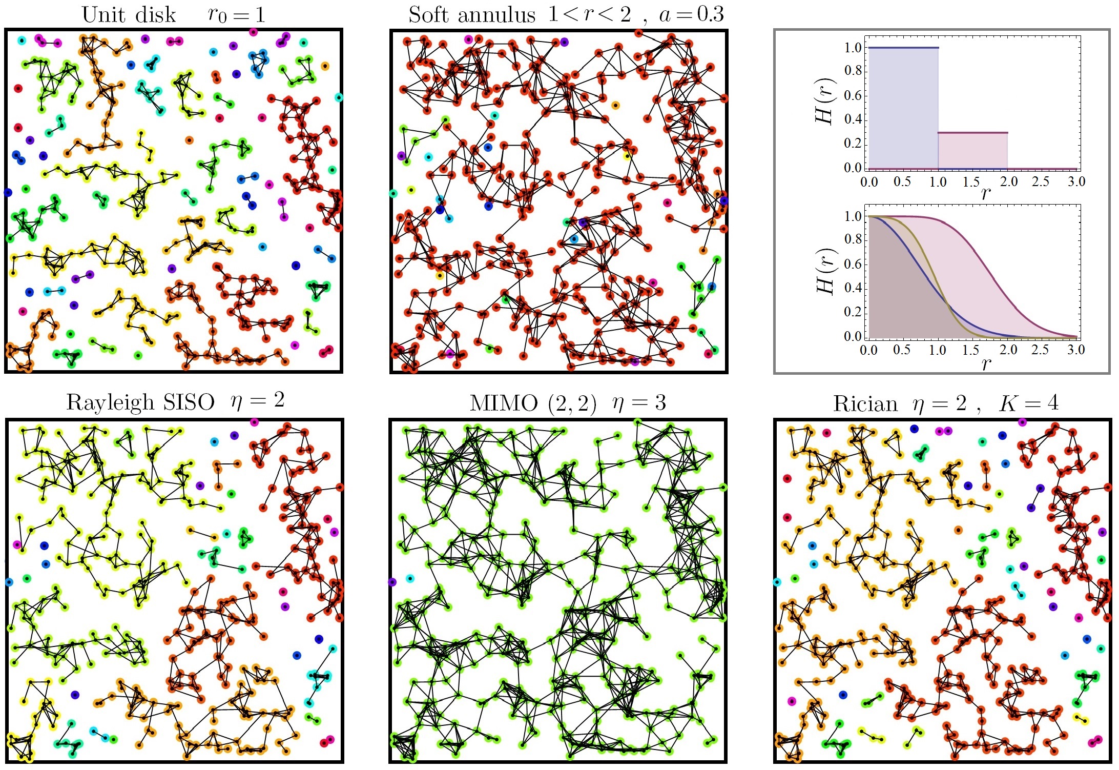
Figure 1: Networks of $N=400$ nodes in a square domain of side $L=20$ resulting from five different connection functions using the same random seed. Clusters of nodes are colour coded. In the top right panel we plot these five $H(r)$ functions in the respective panels. In the lower three we use $\beta=1$.

Fig. 1 shows the effects of several connection functions in forming a RGG; note the striking differences in network topologies. In the simulations, spatial coordinates for $N$ nodes are chosen at random inside a square domain. Nodes $i$ and $j$ are then paired with independent probabilities $H(r_{ij})$. The resulting links are stored in a symmetric zero-one adjacency matrix, and a depth-first search algorithm identifies the connected components of the graph, a process of complexity order $\mathcal{O}(N\ln N)$. For Fig. 1 we use the same random seed as to allow comparison between the different $H(r)$ functions as plotted in the top right panel of Fig. 1, however the process can be repeated in a Monte Carlo fashion (with random seeds) and for different values of $\rho=N/V$ to generate Fig. 6 below.

II.2 Assumptions and notation

Based on these existing examples, we make the following assumptions:

1. Near the origin, $H(r)$ is described by the expansion

   $$H(r)=H(0)+\sum_{\alpha\in{\cal A}}a_{\alpha}r^{\alpha}$$ (7)

   where ${\cal A}\subset(0,\infty)$ has a positive lower bound on the gap size. The minimum of $\cal A$ is denoted $\alpha_{min}$.

2. $H(r)$ is piecewise smooth, with non-smooth points at a discrete and possibly empty set $\{r_{k}\}$, $k\in{\cal K}$, also with a positive lower bound on the gap size.

3. The bulk connectivity mass

   $$M_{d,0}=\left\{\begin{array}[]{cc}2\pi\int H(r)rdr&d=2\\ 4\pi\int H(r)r^{2}dr&d=3\end{array}\right.$$ (8)

   is finite.

4. All derivatives of $H(r)$ are monotonic for sufficiently large $r$.

Remarks: We have $H(0)\in[0,1]$ in all cases. In the case of log-normal fading, corrections for small $r$ are smaller than any power of $r$, ie the expansion is just $H(0)$. If the connectivity mass is finite but $H(r)$ decays very slowly at infinity, some of the local assumptions (and hence Eq. 1) may fail; Mao and Anderson Mao and Anderson (2012) insist on $H(r)=o(r^{-2}\ln(r)^{-2})$ at infinity, which is slightly stronger than finite connectivity mass in $d=2$, for some of their results, but we are mostly interested in exponential decay. The final assumption is to ensure sufficiently rapid decay of the derivatives of $H(r)$ at infinity.

The function $H(r)$ describes the link probability on a line passing through a particular node; we will need various moments of this:

$$H_{m} = \int_{0}^{\infty}H(r)r^{m}dr$$

$$H_{m}^{\prime} = \int_{0}^{\infty}H^{\prime}(r)r^{m}dr$$ (9)

$$H_{m}^{\prime\prime} = \int_{0}^{\infty}H^{\prime\prime}(r)r^{m}dr$$

Integration by parts gives $H_{m}^{\prime}=-mH_{m-1}$ for $m>0$ and $H_{m}^{\prime\prime}=m(m-1)H_{m-2}$ for $m>1$, however the form of $H(r)$ implies that $H_{m}^{\prime}$ and $H_{m}^{\prime\prime}$ have a greater range of validity, since the constant $H(0)$ is removed by differentiation: Our assumptions imply that $H_{m}$ is defined for $-1<m\leq d-1$, $H_{m}^{\prime}$ is defined for $-\alpha_{min}<m\leq d$ and $H_{m}^{\prime\prime}$ is defined for $1-\alpha_{min}<m\leq d+1$. Where there is an explicit formula for non-integer $H_{m}$ and hence for sufficiently large $m$ for $H_{m}^{\prime}$ and $H_{m}^{\prime\prime}$, it may be used to analytically continue the expression to lower $m$; examples are given in Sec. VI below.

The moments may be considered as a Mellin transform evaluated at particular values which depend on the path loss exponent $\eta$. So, if we have $H(r)=g(\beta r^{\eta})$ for some scaled function $g$, a straightforward change of variables gives

$$H_{s-1}=\frac{1}{\eta\beta^{s/\eta}}\{{\cal M}g\}\left(\frac{s}{\eta}\right)$$ (10)

where

$$\{{\cal M}g\}(u)=\int_{0}^{\infty}t^{u-1}g(t)dt$$ (11)

is the Mellin transform of the function $g$.

Occasionally we also define incomplete versions of the moments

$$H_{m}(\epsilon)=\int_{\epsilon}^{\infty}H(r)r^{m}dr$$ (12)

and similarly for the primed versions.

We will also need to define contributions from discontinuities,

$$\Delta_{m} = \sum_{k\in{\cal K}}r_{k}^{m}\left[H(r_{k}+)-H(r_{k}-)\right]$$ (13)

$$\Delta_{m}^{\prime} = \sum_{k\in{\cal K}}r_{k}^{m}\left[H^{\prime}(r_{k}+)-H^{\prime}(r_{k}-)\right]$$ (14)

For the most general calculations we use the further notation

$$\tilde{H}_{-2} = \left\{\begin{array}[]{lc}H_{-1}^{\prime}+\Delta_{-1}&\alpha_{min}>1\\ \displaystyle\lim_{\epsilon\to 0}\left(H_{-1}^{\prime}(\epsilon)+a_{1}\ln\left(|a_{1}|\epsilon\right)+\displaystyle\sum_{\alpha\neq 1}a_{\alpha}\frac{\alpha\epsilon^{\alpha-1}}{\alpha-1}\right)+\Delta_{-1}&\alpha_{min}\leq 1\end{array}\right.$$ (17)

$$3\tilde{H}_{-4} = \left\{\begin{array}[]{lc}H_{-2}^{\prime\prime}-H_{-3}^{\prime}+\Delta_{-2}^{\prime}+\Delta_{-3}&\alpha_{min}>3\\ &\\ \displaystyle\lim_{\epsilon\to 0}\left(H_{-2}^{\prime\prime}(\epsilon)-H_{-3}^{\prime}(\epsilon)+3a_{3}\ln\left(|a_{3}|^{1/3}\epsilon\right)+\displaystyle\sum_{\alpha\neq 3}a_{\alpha}\frac{\alpha(\alpha-2)\epsilon^{\alpha-3}}{(\alpha-3)}\right)+\Delta_{-2}^{\prime}+\Delta_{-3}&\alpha_{min}\leq 3\end{array}\right.$$ (21)

It turns out, however, that in most cases we need the expansions only to second order in the small parameter, and can also assume $\alpha_{min}>1$ (except for the Waxman model). In this case most of the technical details can be avoided, and we find that $\tilde{H}_{-2}$ is given only by the first option, $\tilde{H}_{-4}$ is not needed at all, and terms involving $a_{\alpha}$ (including the hypergeometric functions below) are also not required. So, the reader can safely omit these terms at first sight, and consider them only when a fuller and more general understanding is required.

Figure 2: (a) Geometry for the connectivity mass of a wedge, with the node at the indicated point. We split the domain into two wedges, each with the node located at the edge. (b) The resulting wedge is further split into three parts.

III Connectivity mass

III.1 Integration on a non-centred line

The computation of connection probability, Eq. (1) for moderate to large density is dominated by contributions from the bulk and various boundary components. Each boundary component is controlled by the form of the connectivity mass at and near the boundary, the calculation to which we turn first. This subsection deals with the first integral of $H(r)$, that on an off-centre line, that is needed for the calculations in the later subsections, on the 2D and 3D connectivity mass, respectively.

The connection function is first integrated on a line passing a small distance $x>0$ from the node:

$$F(x)=\int_{0}^{\infty}H(\sqrt{x^{2}+t^{2}})dt$$ (22)

If $\alpha_{min}>3$ we can expand for small $x$ to get

$$F(x) = H_{0}+\frac{x^{2}}{2}[H_{-1}^{\prime}+\Delta_{-1}]$$

$$+\frac{x^{4}}{8}[H_{-2}^{\prime\prime}-H_{-3}^{\prime}+\Delta_{-2}^{\prime}+\Delta_{-3}]+o(x^{4})$$

This may be derived by splitting the integral at the discontinuities, differentiating the result (including integrand and limits) with respect to $x^{2}$ to get the coefficients of the Taylor series.

If $\alpha_{min}\leq 3$ the integrals $H_{-3}^{\prime}$ and $H_{-2}^{\prime\prime}$ diverge, and if $\alpha_{min}\leq 1$ the integral $H_{-1}^{\prime}$ also diverges. In this case we need to split the integrals at a point $\epsilon\ll 1$, and use the small $r$ expansion of $H(r)$ to treat the contribution near the origin separately. We require that $\epsilon$ is much larger than any positive power of $x$; formally we take the limit $x\to 0$ and only then $\epsilon\to 0$. By analogy with the incomplete gamma function, we denote

$$f(x,\epsilon) = \int_{0}^{\epsilon}H(\sqrt{x^{2}+t^{2}})dt$$ (24)

$$F(x,\epsilon) = \int_{\epsilon}^{\infty}H(\sqrt{x^{2}+t^{2}})dt$$ (25)

For $f(x,\epsilon)$, make a change of variable:

$$f(x,\epsilon) = \int_{1}^{\sqrt{(\epsilon^{2}/x^{2})+1}}H(xs)\frac{xs\;ds}{\sqrt{s^{2}-1}}$$ (26)

$$s = \sqrt{(t^{2}/x^{2})+1}$$

Then, expanding for small $x$ (at fixed $\epsilon$) we have

$$f(x,\epsilon) = H(0)\epsilon+\sum_{\alpha}a_{\alpha}f_{\alpha}(x,\epsilon)$$ (27)

$$f_{\alpha}(x,\epsilon) = \frac{\sqrt{\pi}}{2}\frac{\Gamma(-\frac{\alpha+1}{2})}{\Gamma(-\frac{\alpha}{2})}x^{\alpha+1}+\frac{\epsilon^{\alpha+1}}{\alpha+1}+\frac{\alpha\epsilon^{\alpha-1}}{2(\alpha-1)}x^{2}$$

$$+\frac{\alpha(\alpha-2)\epsilon^{\alpha-3}}{8(\alpha-3)}x^{4}+o(x^{4})$$

except that if any of the $\alpha$ are odd integers two of the terms diverge and are replaced by a logarithm:

$$f_{1}(x,\epsilon) = \frac{\epsilon^{2}}{2}+\frac{1}{2}\ln\left(\frac{2\sqrt{e}\epsilon}{x}\right)x^{2}+\frac{x^{4}}{16\epsilon^{2}}+o(x^{4})$$

$$f_{3}(x,\epsilon) = \frac{\epsilon^{4}}{4}+\frac{3\epsilon^{2}}{4}x^{2}+\frac{3}{8}\ln\left(\frac{2e^{3/4}\epsilon}{x}\right)x^{4}+o(x^{4})$$

For even integers (for example the well-studied case $H(r)=e^{-r^{2}}$), the $x^{\alpha+1}$ term is zero, and the series is finite.

The upper integral $F(x,\epsilon)$ has the same expansion as Eq. (III.1), but with incomplete moments $H_{m}(\epsilon)$, $H_{m}^{\prime}(\epsilon)$ and $H_{m}^{\prime\prime}(\epsilon)$.

Putting it back together, we have

$$F(x)=H(0)\epsilon+\sum_{\alpha}a_{\alpha}f_{\alpha}(x,\epsilon)+H_{0}(\epsilon)+\frac{x^{2}}{2}[H_{-1}^{\prime}(\epsilon)+\Delta_{-1}]+\frac{x^{4}}{8}[H_{-2}^{\prime\prime}(\epsilon)-H_{-3}^{\prime}(\epsilon)+\Delta_{-2}^{\prime}+\Delta_{-3}]+o(x^{4})$$ (28)

Note that $F(x)$ does not depend on $\epsilon$: All $\epsilon$ where the relevant series converge should be equivalent, and in particular we may set $\epsilon=0$ where possible to reconstitute the full moment, and otherwise take the limit of a regularised version. So, collecting terms by powers of $x$ we have finally

$$F(x)=H_{0}+\frac{x^{2}}{2}\left[\tilde{H}_{-2}+a_{1}\ln\left(\frac{2\sqrt{e}}{|a_{1}|x}\right)\right]+\frac{3x^{4}}{8}\left[\tilde{H}_{-4}+a_{3}\ln\left(\frac{2e^{3/4}}{|a_{3}|^{1/3}x}\right)\right]+\sum_{\alpha\not\in\{1,3\}}a_{\alpha}\frac{\sqrt{\pi}}{2}\frac{\Gamma(-\frac{\alpha+1}{2})}{\Gamma(-\frac{\alpha}{2})}x^{\alpha+1}+o(x^{4})$$ (29)

where $a_{1}$ and/or $a_{3}$ are deemed to be zero if they do not appear in the expansion of $H(r)$. If they do appear, $|a_{1}|$ and $|a_{3}|^{1/3}$ are included to ensure that the argument of each logarithm is dimensionless. An $a_{2}$ term contributes only at order $x^{2}$: Both $x^{3}$ and $x^{4}$ coefficients vanish. Note that if there are no discontinuities, $\tilde{H}_{-2}$ and $\tilde{H}_{-4}$ correspond to the continuation of the integration by parts expression of $H_{-2}$ and $H_{-4}$ (respectively) to negative index.

III.2 Connectivity mass of polygons

Here we find expansions for the connectivity mass defined in Eq. (2) on and near the boundary. We will use $M_{d,i}$ to denote the mass near a boundary where $d$ is the dimension and $i$ the boundary codimension. The dependence of $M_{d,i}$ on variables may be implicit in the notation; in general it may depend on a parameter (for example the wedge angle) as well as the node location in an appropriate coordinate system.

This section deals with $d=2$, while the next deals with $d=3$. We consider a wedge of total angle $\omega$ and node position in polar coordinates $(r,\phi)$ with connectivity mass denoted $M_{2,2}^{\omega}(r,\phi)$. Using first the simplified geometry of Fig. 2 with $\xi$ a small parameter and (for now) the node on the boundary, the connectivity mass is the sum of three contributions A, B and C as follows:

$$M_{2,2}^{\theta}(\xi\csc\theta,0) = M_{2A}+M_{2B}+M_{2C}$$ (30)

$$M_{2A} = \int_{0}^{\theta}d\phi\int_{0}^{\infty}H(r)rdr=\theta H_{1}$$ (31)

$$M_{2B} = \int_{0}^{\xi}dx\int_{0}^{\infty}dtH(\sqrt{x^{2}+t^{2}})$$ (32)

$$= \int_{0}^{\xi}dxF(x)$$

$$M_{2C} = \int_{0}^{\xi}dx\int_{0}^{x\cot\theta}dtH(\sqrt{x^{2}+t^{2}})$$ (33)

$$= \int_{0}^{\xi}dxf(x,x\cot\theta)$$

where the $2$ in $2A$ etc. denotes the dimension. $M_{2B}$ may be found by integrating the expressions in the previous section, noting that $\xi$, and hence $x$, is small. For $M_{2C}$, we have $x$ small, but we do not have $x\cot\theta\gg x$, so the previous separation between $\epsilon$ and $x$ does not apply. Instead, integrate Eq. (26) directly to obtain $f(x,x\cot\theta)$ and hence

$$M_{2C} = \sum_{\alpha\not\in\{1,3\}}a_{\alpha}\xi^{\alpha+2}\left[\frac{\sqrt{\pi}\Gamma(\frac{-1-\alpha}{2})}{2(\alpha+2)\Gamma(\frac{-\alpha}{2})}+\right.\left.\frac{\csc^{\alpha+1}\theta}{(\alpha+1)(\alpha+2)}\;\>F_{2\hskip 5.0pt1}\left(\frac{1}{2},\frac{-1-\alpha}{2},\frac{1-\alpha}{2},\sin^{2}\theta\right)\right]$$

$$+\frac{H(0)\xi^{2}}{2}\frac{\cos\theta}{\sin\theta}+\frac{a_{1}\xi^{3}}{6}\left[\frac{\cos\theta}{\sin^{2}\theta}+\ln\frac{1+\cos\theta}{\sin\theta}\right]+\frac{a_{3}\xi^{5}}{40}\left[\frac{\cos\theta}{\sin^{2}\theta}\left(3+\frac{2}{\sin^{2}\theta}\right)+3\ln\frac{1+\cos\theta}{\sin\theta}\right]+o(\xi^{5})$$

Thus, for the whole wedge we have

$$M_{2,2}^{\theta}(\xi\csc\theta,0) = \theta H_{1}+\xi H_{0}+\xi^{2}\frac{H(0)}{2}\frac{\cos\theta}{\sin\theta}+\frac{\xi^{3}}{6}\left[\tilde{H}_{-2}+a_{1}\left(\frac{\cos\theta}{\sin^{2}\theta}+\ln\frac{1+\cos\theta}{\sin\theta}+\ln\left(\frac{2e^{5/6}}{|a_{1}|\xi}\right)\right)\right]$$

$$+\frac{\xi^{5}}{40}\left[3\tilde{H}_{-4}+a_{3}\left(\frac{\cos\theta}{\sin^{2}\theta}\left(3+\frac{2}{\sin^{2}\theta}\right)+3\ln\frac{1+\cos\theta}{\sin\theta}+3\ln\left(\frac{2e^{19/20}}{|a_{3}|^{1/3}\xi}\right)\right)\right]$$

$$+\sum_{\alpha\not\in\{1,3\}}a_{\alpha}\xi^{\alpha+2}\left[\frac{\sqrt{\pi}\Gamma(\frac{-1-\alpha}{2})}{2(\alpha+2)\Gamma(\frac{-\alpha}{2})}+\right.\left.\frac{\csc^{\alpha+1}\theta}{(\alpha+1)(\alpha+2)}\;\>F_{2\hskip 5.0pt1}\left(\frac{1}{2},\frac{-1-\alpha}{2},\frac{1-\alpha}{2},\sin^{2}\theta\right)\right]+o(\xi^{5})$$

There are special values of the hypergeometric function for even $\alpha$:

$$\left.F_{2\hskip 5.0pt1}\left(\frac{1}{2},\frac{-1-\alpha}{2},\frac{1-\alpha}{2},\sin^{2}\theta\right)\right|_{\alpha=2} = \cos\theta(3-\cos^{2}\theta)$$ (36)

$$\left.F_{2\hskip 5.0pt1}\left(\frac{1}{2},\frac{-1-\alpha}{2},\frac{1-\alpha}{2},\sin^{2}\theta\right)\right|_{\alpha=4} = \frac{1}{3}\cos\theta(15-20\cos^{2}\theta+8\cos^{4}\theta)$$ (37)

and for limiting angles

$$\left.F_{2\hskip 5.0pt1}\left(\frac{1}{2},\frac{-1-\alpha}{2},\frac{1-\alpha}{2},\sin^{2}\theta\right)\right|_{\theta=0} = \left.F_{2\hskip 5.0pt1}\left(\frac{1}{2},\frac{-1-\alpha}{2},\frac{1-\alpha}{2},\sin^{2}\theta\right)\right|_{\theta=\pi}=1$$ (38)

$$\left.F_{2\hskip 5.0pt1}\left(\frac{1}{2},\frac{-1-\alpha}{2},\frac{1-\alpha}{2},\sin^{2}\theta\right)\right|_{\theta=\frac{\pi}{2}} = \frac{\sqrt{\pi}\Gamma(\frac{1-\alpha}{2})}{\Gamma(\frac{-\alpha}{2})}$$ (39)

Thus the two terms in the sum over $\alpha$ cancel when $\theta=\pi/2$.

Combining two wedges, we have the connectivity mass at a general point of a wedge of angle (and solid angle) $\omega$, with the node at polar point $(r,\theta)$:

$$M_{2,2}^{\omega}(r,\theta) = M_{2,2}^{\theta}(r,0)+M_{2,2}^{\theta^{\prime}}(r,0)$$ (41)

$$= \omega H_{1}+rH_{0}[\sin\theta+\sin\theta^{\prime}]+\frac{H(0)r^{2}}{2}[\sin\theta\cos\theta+\sin\theta^{\prime}\cos\theta^{\prime}]$$

$$+\frac{\tilde{H}_{-2}r^{3}}{6}[\sin^{3}\theta+\sin^{3}\theta^{\prime}]+\frac{3\tilde{H}_{-4}r^{5}}{40}[\sin^{5}\theta+\sin^{5}\theta^{\prime}]+O(r^{\alpha_{min}+2}\ln r)+o(r^{5})$$

where $\theta^{\prime}=\omega-\theta$ and omitted terms involving $a_{\alpha}$ can be found from Eq. (III.2) above.

An important special case is that of an edge, $M_{2,1}$ where $\omega=\pi$ and we may take $\theta=\pi/2$, and so the $a_{\alpha}$ terms cancel. The above expressions reduce to

$$M_{2,1}(r) = \pi H_{1}+2rH_{0}+\frac{r^{3}}{3}\left[\tilde{H}_{-2}+a_{1}\ln\left(\frac{2e^{5/6}}{|a_{1}|r}\right)\right]+\frac{3r^{5}}{20}\left[\tilde{H}_{-4}+a_{3}\ln\left(\frac{2e^{19/20}}{|a_{3}|^{1/3}r}\right)\right]+o(r^{5})$$ (42)

Together with the bulk connectivity mass $M_{2,0}=2\pi H_{1}$ we have all the ingredients for convex polygons.

III.3 Connectivity mass of polyhedra

Here, we find the connectivity mass near the boundary in three dimensional geometries. The connectivity mass of the bulk is $M_{3,0}=4\pi H_{2}$. For a node a small distance $r$ from a face we use cylindrical coordinates and a transformation $s=\sqrt{x^{2}+\rho^{2}}$ in the second line:

$$M_{3,1}(r) = \int_{-r}^{\infty}dx\int_{0}^{\infty}\rho\;d\rho\int_{0}^{2\pi}d\theta\;H(\sqrt{x^{2}+\rho^{2}})$$

$$= M_{3,1}(0)+2\pi\int_{0}^{r}dx\int_{x}^{\infty}ds\;sH(s)$$

$$= 2\pi H_{2}+2\pi\int_{0}^{r}dx\left[H_{1}-\int_{0}^{x}ds\;sH(s)\right]$$

$$= 2\pi\left[H_{2}+rH_{1}-\frac{r^{3}H(0)}{6}-\sum_{\alpha}a_{\alpha}\frac{r^{3+\alpha}}{(\alpha+2)(\alpha+3)}\right]$$

For an edge in 3D of angle $\theta$, use the same splitting and coordinates as in Fig. 2, that is, first consider a node on the boundary, then the interior case consists of two combined 3D wedges. Noting that the solid angle is $2\theta$, we find

$$M_{3,2}^{\theta}(\xi\csc\theta,0) = M_{3A}+M_{3B}+M_{3C}$$ (44)

$$M_{3A} = 2\theta H_{2}$$ (45)

$$M_{3B} = \pi\left[\xi H_{1}-\frac{\xi^{3}H(0)}{6}-\sum_{\alpha}a_{\alpha}\frac{\xi^{3+\alpha}}{(\alpha+2)(\alpha+3)}\right]$$ (46)

Note that the $B$ region is half the slab considered for the face above. Using cylindrical coordinates we have

$$M_{3C} = \int_{0}^{\pi/2-\theta}\int_{0}^{\xi\sec\phi}\int_{-\infty}^{\infty}\rho H(\sqrt{\rho}^{2}+z^{2})dzd\rho d\phi$$

$$= 2\int_{0}^{\pi/2-\theta}\int_{0}^{\xi\sec\phi}\rho F(\rho)d\rho d\phi$$

$$= \int_{0}^{\pi/2-\theta}\left\{H_{0}\xi^{2}\sec^{2}\phi+\frac{\xi^{4}\sec^{4}\phi}{4}\left[\tilde{H}_{-2}+a_{1}\ln\left(\frac{2e^{3/4}}{|a_{1}|\xi\sec\phi}\right)\right]+\sum_{\alpha\neq 1}\frac{a_{\alpha}\sqrt{\pi}}{3+\alpha}\frac{\Gamma(-\frac{\alpha+1}{2})}{\Gamma(-\frac{\alpha}{2})}\xi^{3+\alpha}\sec^{3+\alpha}\phi\right\}d\phi$$

$$+o(\xi^{4})$$

$$= H_{0}\xi^{2}\cot\theta+\frac{\xi^{4}}{4}(\cot\theta+\frac{\cot^{3}\theta}{3})\left[\tilde{H}_{-2}+a_{1}\ln\left(\frac{2e^{3/4}}{|a_{1}|\xi\csc\theta}\right)\right]$$

$$+\sum_{\alpha\neq 1}\frac{a_{\alpha}\sqrt{\pi}}{3+\alpha}\frac{\Gamma(-\frac{\alpha+1}{2})}{\Gamma(-\frac{\alpha}{2})}\xi^{3+\alpha}\cos\theta\hskip 5.0ptF_{2\hskip 5.0pt1}\left(\frac{1}{2},\frac{4+\alpha}{2},\frac{3}{2},\cos^{2}\theta\right)+o(\xi^{4})$$

Thus the combined edge contribution is

$$M_{3,2}^{\theta}(\xi\csc\theta,0)=2\theta H_{2}+\xi\pi H_{1}+\xi^{2}H_{0}\cot\theta-\frac{\xi^{3}\pi H(0)}{6}+\frac{\xi^{4}\tilde{H}_{-2}}{12}(3\cot\theta+\cot^{3}\theta)+O(\xi^{\alpha_{min}+3}\ln\xi)+o(\xi^{4})$$ (48)

with omitted terms given in Eqs. (46,III.3). As in the 2D case, we can now treat a general point (polar coordinates $(r,\theta)$) near an edge of angle $\omega$ (and hence solid angle $2\omega$) as a sum of two such contributions, leading to

$$M_{3,2}^{\omega}(r,\theta) = M_{3,2}^{\theta}(r,0)+M_{3,2}^{\theta^{\prime}}(r,0)$$

$$= 2\omega H_{2}+r\pi H_{1}\left[\sin\theta+\sin\theta^{\prime}\right]+r^{2}H_{0}\left[\sin\theta\cos\theta+\sin\theta^{\prime}\cos\theta^{\prime}\right]-\frac{\pi r^{3}H(0)}{6}[\sin^{3}\theta+\sin^{3}\theta^{\prime}]$$

$$+\frac{r^{4}\tilde{H}_{-2}}{12}[3\sin^{3}\theta\cos\theta+\sin\theta\cos^{3}\theta+3\sin^{3}\theta^{\prime}\cos\theta^{\prime}+\sin\theta^{\prime}\cos^{3}\theta^{\prime}]+O(r^{\alpha_{min}+3}\ln r)+o(r^{4})$$

where $\theta^{\prime}=\omega-\theta$.

Figure 3: Geometry for the connectivity mass of a 3D corner, with the node at the indicated point and the section between it and the corner cut away. The quantities $\xi$, $\eta$, $\zeta$ denote the perpendicular distances to the three faces. The domain is split into eight pieces, uniquely labelled by which of these are relevant, for example $M_{\xi\eta\zeta}$ is the connectivity mass of the piece that was cut away, and $M_{\xi\eta}$ is a semi-infinite kite shaped prism.

Finally we consider a node near a right angled vertex, with angle and solid angle $\omega$, and located at $(r,\theta,\zeta)$ in cylindrical coordinates; the distance to the angled planes are as before $\xi=r\sin\theta$ and $\eta=r\sin\theta^{\prime}$: See Fig. 3. The connectivity mass is obtained by combining previous results for eight regions, for which we keep terms up to and including third order in the small quantities $\xi$, $\eta$ and $\zeta$:

$$M_{3,3}^{\omega}(r,\theta,\zeta)=M_{.}+M_{\xi}+M_{\eta}+M_{\zeta}+M_{\xi\eta}+M_{\xi\zeta}+M_{\eta\zeta}+M_{\xi\eta\zeta}$$ (50)

Here,

$$M_{.}=\omega H_{2}$$ (51)

is from the interior region obtained by translating the vertex so that it coincides with the node,

$$M_{\xi}=\frac{\pi}{2}\left[\xi H_{1}-\frac{\xi^{3}}{6}H(0)+\ldots\right]$$ (52)

is from a quarter slab of width $\xi$, and similarly $M_{\eta}$; see the face contribution above.

$$M_{\zeta}=\omega\left[\zeta H_{1}-\frac{\zeta^{3}}{6}H(0)+\ldots\right]$$ (53)

is from a similar slab with an angle $\omega$ rather than $\pi/2$.

$$M_{\xi\eta} = \frac{1}{2}\left[M_{C3}(\theta,\xi)+M_{C3}(\theta^{\prime},\eta)\right]$$ (54)

$$= \frac{H_{0}}{2}\left[\xi^{2}\cot\theta+\eta^{2}\cot\theta^{\prime}\right]+\ldots$$

is from a semi-infinite strip with cross-section formed by two right angled triangles with common hypotenuse $r$ and angles $\theta$ and $\theta^{\prime}$ respectively.

$$M_{\xi\zeta} = \frac{1}{2}\left[M_{C3}(\arctan(\xi/\zeta),\xi)+M_{C3}(\arctan(\zeta/\xi),\zeta)\right]$$ (55)

$$= H_{0}\xi\zeta+\ldots$$

is from a semi-infinite strip with rectangular cross-section of lengths $\xi$ and $\zeta$, that may be split into two right-angled triangles along the diagonal, and similarly for $M_{\eta\zeta}$. Finally

$$M_{\xi\eta\zeta}=\frac{H(0)}{2}\zeta r^{2}\left[\sin\theta\cos\theta+\sin\theta^{\prime}\cos\theta^{\prime}\right]+\ldots$$ (56)

is from a prism with the same cross-section as $M_{\xi\eta}$ and length $\zeta$; since its extent is small in all directions its contribution (to third order) is given by $H(0)$ multiplied by its volume. Putting this together and expressing $\xi$ and $\eta$ in terms of $r$ and $\theta$ we have

$$M_{3,3}^{\omega}(r,\theta,\zeta) = \omega H_{2}+\left[\frac{\pi}{2}r(\sin\theta+\sin\theta^{\prime})+\omega\zeta\right]H_{1}+\left[\frac{r^{2}}{2}(\sin\theta\cos\theta+\sin\theta^{\prime}\cos\theta^{\prime})+r\zeta(\sin\theta+\sin\theta^{\prime})\right]H_{0}$$ (57)

$$-\left[\pi r^{3}(\sin^{3}\theta+\sin^{3}\theta^{\prime})-6r^{2}\zeta(\sin\theta\cos\theta+\sin\theta^{\prime}\cos\theta^{\prime})+2\omega\zeta^{3}\right]\frac{H(0)}{12}+o(r^{3},\zeta^{3})$$

where again $\theta^{\prime}=\omega-\theta$. As expected, we have $M_{3,2}^{\omega}(r,\theta)=2M_{3,3}^{\omega}(r,\theta,0)$ and $M_{3,1}(r)=M_{3,2}^{\pi}(r,\pi/2)$.

IV Connection probability

IV.1 Separation into boundary components

Having obtained the connectivity mass in the vicinity of various boundaries in two and three dimensions, we are now in a position to evaluate Eq. (1) asymptotically (using Laplace’s method) for large $\rho$, and system size $L$, summing the dominant bulk and/or boundary contributions leading to Eq. (4). We do not have a fully rigorous justification for this separation, however the neglect of contributions from intermediate regions may be justified as follows (in two dimensions; we expect three dimensions to be similar):

Split the integration region $\cal V$ of the outer integral appearing in Eq. (1) into regions by lines a distance $\epsilon_{1}$ and a distance $\epsilon_{2}$ from the boundary. We will take $\rho$ and $L$ large, then choose $\frac{\ln\rho}{\rho}\ll\epsilon_{1}\ll 1$ and $1\ll\epsilon_{2}\ll L$. Then, the contribution from the intermediate regions (ie a distance from the boundary between $\epsilon_{1}$ and $\epsilon_{2}$) can be estimated, and is always of a lower order than at least one of the main (corner, edge, bulk) contributions. For example, the edge contribution in two dimensions (Eq. (65) below) is of the form

$$P_{2,1}=Pe^{\rho\pi H_{1}}(1+o(1))$$ (58)

where $P$ is the perimeter, proportional to $L$; this corresponds to a region in which the distance to an edge is less than $\epsilon_{1}$, but the distance to other edges is greater than $\epsilon_{2}$. Comparing with the bulk and corner contributions, this dominates when

$$\rho^{-1}e^{\rho(\pi-\omega)H_{1}}\lesssim L\lesssim\rho^{-1}e^{\rho\pi H_{1}}$$ (59)

There are three intermediate regions, where one or both of these distances is in $[\epsilon_{1},\epsilon_{2}]$. Taking the region where both are in this range $I_{wb}$ near a corner of angle $\omega$ for example, we can estimate it by

$$I_{wb}\lesssim\rho e^{-\rho(\omega H_{1}+2\epsilon_{1}\sin(\omega/2)H_{0})}$$ (60)

using the connectivity mass at the point closest the corner (an angle $\omega/2$), Eq. (41). So, we find that under our assumptions $P_{2,1}\gg I_{wb}$. The other combinations of regimes may be estimated similarly, leading to the conclusion that in all cases, one of the bulk, edge or corner contributions dominates all three intermediate contributions. We expect a similar analysis to work in three dimensions also. So formally we conjecture that (compare with Eq. 4)

$$\frac{1-P_{fc}}{\sum_{i}\sum_{b\in{\cal B}_{i}}\rho^{1-i}G_{d,i}^{(b)}V_{b}e^{-\rho\Omega_{b}H_{d-1}}}\to 1$$ (61)

in any limit where both $\rho$ and $L$ go to infinity. Including terms in the denominator that are subleading in $\rho$ will not change the result, but should improve the rate of convergence.

IV.2 Polygons

We now present the results of Laplace’s method for expanding Eq. (1) for large $\rho$ in the two dimensional case; three dimensions is considered in the next section. For convex polygons we have the following results from Sec. III.2 above:

$$M_{2,0} = 2\pi H_{1}$$

$$M_{2,1}(r) = \pi H_{1}+2rH_{0}$$

$$+\frac{r^{3}}{3}\left[\tilde{H}_{-2}+a_{1}\ln\left(\frac{2e^{5/6}}{|a_{1}|r}\right)\right]+o(r^{3})$$

$$M_{2,2}(\omega;r,\theta) = \omega H_{1}+r[\sin\theta+\sin\theta^{\prime}]H_{0}$$

$$+\frac{H(0)r^{2}}{2}[\sin\theta\cos\theta+\sin\theta^{\prime}\cos\theta^{\prime}]$$

$$+O(r^{3}\ln r,r^{2+\alpha_{min}})$$

where $\omega$ is the angle of the corner, $(r,\theta)$ are polar coordinates of the node position, and other symbols and details are given in the above section. The argument (as yet only semi-rigorous) is that for combined limits $\rho\to\infty$, $L\to\infty$ so that $P_{fc}\to 1$, a sum of boundary contributions takes into account correctly the connectivity mass at locations of order $r_{0}$ from the boundary, which is not explicitly estimated above. We have

$$P_{fc}=1-P_{2,0}-P_{2,1}-\sum_{corners}P_{2,2}$$ (63)

where the corner contributions are separated out to allow for differing angles, while the bulk and edge contributions involve only the total area and perimeter respectively. The bulk contribution is

$$P_{2,0} = \rho\int_{bulk}e^{-\rho M_{bulk}}dxdy$$ (64)

$$= \rho Ae^{-2\pi\rho H_{1}}$$

Here, $A$ is the area. The edge contribution is (using $y$ to denote displacement along the edge and $x$ normal to it)

$$P_{2,1} = \rho\int_{edge}e^{-\rho M_{2,1}(x)}dxdy$$ (65)

$$= \rho P\int_{0}^{\infty}e^{-\rho\left[[\pi H_{1}+2xH_{0}+\frac{x^{3}}{3}\left[\tilde{H}_{-2}+a_{1}\ln\left(\frac{2e^{5/6}}{|a_{1}|x}\right)\right]+O(x^{5}\ln x)\right]}dx$$

$$= \rho Pe^{-\rho\pi H_{1}}\int_{0}^{\infty}e^{-2\rho H_{0}x}\left[1-\frac{\rho x^{3}}{3}\left[\tilde{H}_{-2}+a_{1}\ln\left(\frac{2e^{5/6}}{|a_{1}|x}\right)\right]+O(x^{5}\ln x)\right]dx$$

$$= Pe^{-\rho\pi H_{1}}\left[\frac{1}{2H_{0}}-\frac{\tilde{H}_{-2}+a_{1}\left[\gamma+\ln\left(\frac{4\rho H_{0}}{e|a_{1}|}\right)\right]}{8\rho^{2}H_{0}^{4}}+O(\rho^{-4}\ln\rho)\right]$$

Here, $P$ is the perimeter and $\gamma$ is Euler’s constant. Each corner contribution is

$$P_{2,2}^{\omega} = \rho\int_{w}e^{-\rho M_{2,2}^{\omega}(r,\theta)}rdrd\theta$$

$$= \rho\int_{0}^{\omega}d\theta\int_{0}^{\infty}rdre^{-\rho\left[\omega H_{1}+rH_{0}(\sin\theta+\sin\theta^{\prime})+\frac{H(0)r^{2}}{2}(\sin\theta\cos\theta+\sin\theta^{\prime}\cos\theta^{\prime})+\frac{\tilde{H}_{-2}r^{3}}{6}(\sin^{3}\theta+\sin^{3}\theta^{\prime})+O(r^{\alpha_{min}+2}\ln r,r^{5})\right]}$$

$$= \rho e^{-\rho\omega H_{1}}\int_{0}^{\omega}d\theta\int_{0}^{\infty}rdre^{-\rho rH_{0}(\sin\theta+\sin\theta^{\prime})}$$

$$\left[1-\frac{\rho H(0)r^{2}}{2}(\sin\theta\cos\theta+\sin\theta^{\prime}\cos\theta^{\prime})-\frac{\rho\tilde{H}_{-2}r^{3}}{6}(\sin^{3}\theta+\sin^{3}\theta^{\prime})+O(r^{\alpha_{min}+2}\ln r,r^{4})\right]$$

$$= e^{-\rho\omega H_{1}}\int_{0}^{\omega}d\theta$$

$$\left[\frac{1}{\rho H_{0}^{2}(\sin\theta+\sin\theta^{\prime})^{2}}-\frac{3H(0)(\sin\theta\cos\theta+\sin\theta^{\prime}\cos\theta^{\prime})}{\rho^{2}H_{0}^{4}(\sin\theta+\sin\theta^{\prime})^{4}}-\frac{4\tilde{H}_{-2}(\sin^{3}\theta+\sin^{3}\theta^{\prime})}{\rho^{3}H_{0}^{5}(\sin\theta+\sin\theta^{\prime})^{5}}+O(\rho^{-\alpha_{min}-2}\ln\rho,\rho^{-4})\right]$$

$$= e^{-\rho\omega H_{1}}\left[\frac{1}{\rho H_{0}^{2}\sin\omega}-\frac{H(0)(2\cos\omega+1)}{\rho^{2}H_{0}^{4}\sin^{2}\omega}-\frac{2\tilde{H}_{-2}}{\rho^{3}H_{0}^{5}\sin\omega}+O(\rho^{-\alpha_{min}-2}\ln\rho,\rho^{-4})\right]$$

IV.3 Polyhedra

We can perform the same analysis on 3D shapes, using the results of Sec. III.3. We find

$$P_{fc}=1-P_{3,0}-P_{3,1}-\sum_{edges}P_{3,2}-\sum_{vertices}P_{3,3}$$ (67)

where as above the edge and corner contributions are considered separately to allow for different angles, while the bulk and surface involve only the total volume and surface area respectively. The bulk, surface and edge contributions are, respectively,

$$P_{3,0} = \rho Ve^{-4\pi\rho H_{2}}$$ (68)

$$P_{3,1} = Se^{-2\pi\rho H_{2}}\left[\frac{1}{2\pi H_{1}}+\frac{2\pi H(0)}{\rho^{2}(2\pi H_{1})^{4}}+\sum_{\alpha}\frac{a_{\alpha}\Gamma(2+\alpha)}{\rho^{2+\alpha}(2\pi H_{1})^{4+\alpha}}+O(\rho^{-5})\right]$$ (69)

$$P_{3,2}^{\omega} = Le^{-2\omega\rho H_{2}}\left[\frac{1}{\rho\pi^{2}H_{1}^{2}\sin\omega}-\frac{2H_{0}}{\rho^{2}\pi^{4}H_{1}^{4}}\frac{2\cos\omega+1}{\sin^{2}\omega}+\frac{2\pi H(0)}{\rho^{3}\pi^{5}H_{1}^{5}\sin\omega}+O(\rho^{-\alpha_{min}-3}\ln\rho,\rho^{-4})\right]$$ (70)

where $V$ is the volume, $S$ the surface area and $L$ the length of an edge. For a right-angled vertex of angle $\omega$ we have using the same approach

$$P_{3,3}^{\omega} = \rho\int_{0}^{\infty}d\zeta\int_{0}^{\omega}d\theta\int_{0}^{\infty}rdr$$

$$e^{-\rho\left[\omega H_{2}+(\frac{\pi}{2}r(\sin\theta+\sin\theta^{\prime})+\omega\zeta)H_{1}+(\frac{r^{2}}{2}(\sin\theta\cos\theta+\sin\theta^{\prime}\cos\theta^{\prime})+r\zeta(\sin\theta+\sin\theta^{\prime}))H_{0}+O(r^{3},\zeta^{3})\right]}$$

$$= \rho\int_{0}^{\infty}d\zeta\left[\frac{e^{-\rho\omega(H_{2}+\zeta H_{1})}}{\rho^{2}(\frac{\pi}{2}H_{1}+\zeta H_{0})^{2}\sin\omega}-\frac{H_{0}e^{-\rho\omega(H_{2}+\zeta H_{1})}}{\rho^{3}(\frac{\pi}{2}H_{1}+\zeta H_{0})^{4}}\frac{2\cos\omega+1}{\sin^{2}\omega}+O(\rho^{-4})\right]$$

Noting again that $\rho$ is large and hence that only small $\zeta$ contribute, we expand the denominators in positive powers of $\zeta$ and integrate to give

$$P_{3,3}^{\omega}=e^{-\omega\rho H_{2}}\left[\frac{4}{\rho^{2}H_{1}^{3}\pi^{2}\omega\sin\omega}-\frac{16H_{0}}{\rho^{3}H_{1}^{5}\pi^{4}}\frac{\pi\sin\omega+2\omega\cos\omega+\omega}{\omega^{2}\sin^{2}\omega}+O(\rho^{-4})\right]$$ (72)

IV.4 Leading and nonleading terms

Comparing the 2D and 3D results of the previous sections with the geometrical factor Eq. (4) we find the quantities given in Tab. 1, which are remarkably simple and general, and one of the main results of this paper. In particular, the geometrical factor depends only on the connection function via the $-i$ power of a single integral, namely $H_{d-2}$.

The nonleading terms involve smaller moments and the $a_{\alpha}$, that is, behaviour of the connection function near the origin. Comparing the leading and second terms in the $P_{d,i}^{\omega}$ and noting that $H_{m}$ scales as $r_{0}^{m+1}$ in terms of a typical length scale $r_{0}$, we find they are the same order of magnitude if $\rho r_{0}^{d}$ is of order unity. Physically this corresponds both to the average degree and to the argument of the exponentials. Thus for densities much above this, the terms in the expansions decrease rapidly, as we expect.

There are, however a few caveats. The coefficients of the higher order terms may increase. This is very common in asymptotic results; formally the series may not converge, but in practice the first few terms remain a useful approximation of the function at values of the variable (density) for which they decrease.

A more serious issue occurs for sharp corners. The value of density at which the first two terms of the 2D corner contribution $P_{2,2}^{\omega}$, Eq. (IV.2), are equal is

$$\rho_{eq}=\frac{H(0)}{H_{0}^{2}}\frac{2\cos\omega+1}{\sin\omega}$$ (73)

which increases for sharp angles (small $\omega$), and also angles approaching $\pi$. Thus care must be taken when approximating $P_{2,2}^{\omega}$ at moderate densities. The optimal angle is $2\pi/3$, for which the second term vanishes; this corresponds to a hexagonal domain, popular in cellular networks. The same holds for $P_{3,2}^{\omega}$; for $P_{3,3}^{\omega}$ the term vanishes at a slightly higher angle of approximately $2.56125$ (for example, close to a hendecagonal prism).

V Curvature effects

The previous calculations may be extended to geometries with curved boundaries. If the boundary is smooth, then at sufficiently large system size $L$, we can assume that the radius of curvature is much greater than the connection range, and so treat the curvature as a small parameter. In two dimensions a generic smooth boundary may be taken to have equation

$$z=\frac{\kappa x^{2}}{2}+O(x^{3})$$ (74)

and we place a node at $x=0$, $z=r>0$. This convention makes the curvature $\kappa>0$ for convex domains. Neglecting terms of order $\kappa^{2}$ and $r^{3}$ for consistency, we find the curvature correction

$$-M_{2,1}^{\kappa}(r) = \int_{-\infty}^{\infty}dx\int_{0}^{\kappa x^{2}/2}dzH(\sqrt{x^{2}+(z-r)^{2}})$$

$$= \int_{-\infty}^{\infty}dx\int_{0}^{\kappa x^{2}/2}dz\left[H(x)+\frac{r^{2}}{2x}H^{\prime}(x)+\ldots\right]$$

$$= \kappa\left[H_{2}+\frac{r^{2}}{2}H^{\prime}_{1}+\ldots\right]$$

$$= \kappa\left[H_{2}-\frac{r^{2}}{2}H_{0}+\ldots\right]$$

using the integration by parts formula following Eq. (9). Thus we update the calculation in Eq. (65) to obtain

$$P_{2,1}=Pe^{-\rho(\pi H_{1}-\kappa H_{2})}\left[\frac{1}{2H_{0}}-\frac{\kappa}{8\rho H_{0}^{2}}+O(\rho^{-2})\right]$$ (76)

Notice that the curvature affects the exponential, hence reducing the effective angle slightly below $\pi$. However the leading order geometrical factor remains unchanged.

In three dimensions, the corresponding leading order expression for the boundary is

$$z=\frac{1}{2}\left(\kappa_{1}x^{2}+\kappa_{2}y^{2}\right)+\ldots$$ (77)

where $(\kappa_{1},\kappa_{2})$ are principal curvatures and $(x,y)$ displacements in the corresponding mutually orthogonal directions. Using polar coordinates we have

$$-M_{3,1}^{\kappa}(r) = \int_{0}^{\infty}\rho d\rho\int_{0}^{2\pi}d\theta\int_{0}^{(\kappa_{1}\cos^{2}\theta+\kappa_{2}\sin^{2}\theta)/2}dz$$

$$\times H(\sqrt{\rho^{2}+(z-r)^{2}})$$

$$= \int_{0}^{\infty}\rho d\rho\int_{0}^{2\pi}d\theta\int_{0}^{(\kappa_{1}\cos^{2}\theta+\kappa_{2}\sin^{2}\theta)/2}dz$$

$$\times\left[H(\rho)+\frac{r^{2}}{2}H^{\prime}(\rho)+\ldots\right]$$

$$= \pi\kappa\left(H_{3}+\frac{r^{2}}{2}H^{\prime}_{2}+\ldots\right)$$

$$= \pi\kappa(H_{3}-r^{2}H_{1}+\ldots)$$

where $\kappa=(\kappa_{1}+\kappa_{2})/2$ is the mean curvature. From this we find

$$P_{3,1}=Se^{-\pi\rho(2H_{2}-\kappa H_{3})}\left[\frac{1}{2\pi H_{1}}-\frac{\kappa}{\rho(2\pi H_{1})^{2}}+O(\rho^{-2})\right]$$ (79)

which has a similar structure to the two dimensional case. Note also that it depends only on the mean curvature $\kappa$ and not the individual principal curvatures.

VI Comparison with previous results and numerics

The above expressions for $P_{fc}$ require only a few specific integrals of $H(r)$ for its evaluation, which for commonly used connection functions are given in Tab. 2. Note that the expressions are valid whenever $\tilde{H}_{s-1}$ is defined; for the soft disk/annulus models, the contribution for negative $s$ comes from the discontinuity(-ies), while in the Rayleigh fading case, from continuation of the integration by parts expressions. In the latter, $\tilde{H}_{-2}$ converges only for $\eta>1$ and $\tilde{H}_{-4}$ converges only for $\eta>3$. Some specific values for $\eta=2$ are given in Tab. 3.

We now compare the general results found above with geometric factors in specific cases studied previously, finding agreement with the above results. The Rayleigh SISO model was considered in Ref. Coon et al. (2012b), giving, for $\eta=2$,

$$G_{d,i}^{\pi/2}=2^{i(i-1)}\left(\frac{\beta}{\pi}\right)^{\frac{i(d-1)}{2}}$$ (80)

for bulk, edges/faces and purely right angled corners in either two or three dimensions. A general angle and path loss exponent was also considered in two dimensions:

$$G_{2,2}^{\omega}=\frac{\beta^{2/\eta}}{\sin\omega\Gamma(1+\eta^{-1})^{2}}$$ (81)

The earlier paper Coon et al. (2012a) gave special cases of these, namely $G_{3,i}^{\pi/2}$ and $G_{2,i}^{\omega}$, with a typo for $G_{2,1}^{\omega}$. The other paper with directly comparable results is Ref. Coon et al. (2014). Here, the model is $2\times 2$ MIMO with $\eta=2$, for which $H_{1}$ and $H_{2}$ are given in Tab. 3. Finally, a circular or spherical boundary and Gaussian connection function were considered in Ref. Giles et al. (to be published). In all cases the results agree with the more general expressions herein.

We test Eq. (61) for the case of a square domain of side length $L$ as shown in Fig. 4. The contributions from separate terms can be seen in Fig. 5. For both of these cases, the comparison is between the sum of boundary contributions and numerical integration of Eq. (1). A further test in Fig. 6 compares the sum of boundary contributions with an ensemble of directly simulated random graphs for a variety of connection functions for a triangular domain. Thus it implicitly also confirms the validity of the assumptions undergirding Eq. (1) for these connection functions.

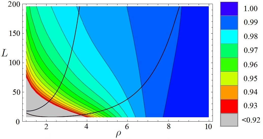
Figure 4: Test of Eq. (61) for a square domain of side length $L$ and node density $\rho$. The expression should tend to $1$ in any limit for which $\rho\to\infty$ and $L\to\infty$. The boundary between regions in which the corners (right), edges (middle) and bulk (left) dominate are shown in black; these appear to have no effect, thus illustrating the uniformity of the expansion.

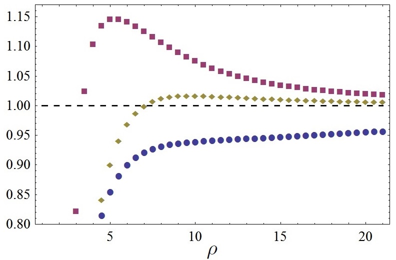
Figure 5: The ratio $\frac{1-P_{fc}-P_{2,0}-P_{2,1}}{P_{2,2}}$ for the square considered in Fig. 4 and side length $L=10$, showing convergence as more terms are included in $P_{2,2}$: Blue circles, purple squares, yellow diamonds to order $\rho^{-1}$, $\rho^{-2}$, $\rho^{-3}$ respectively.

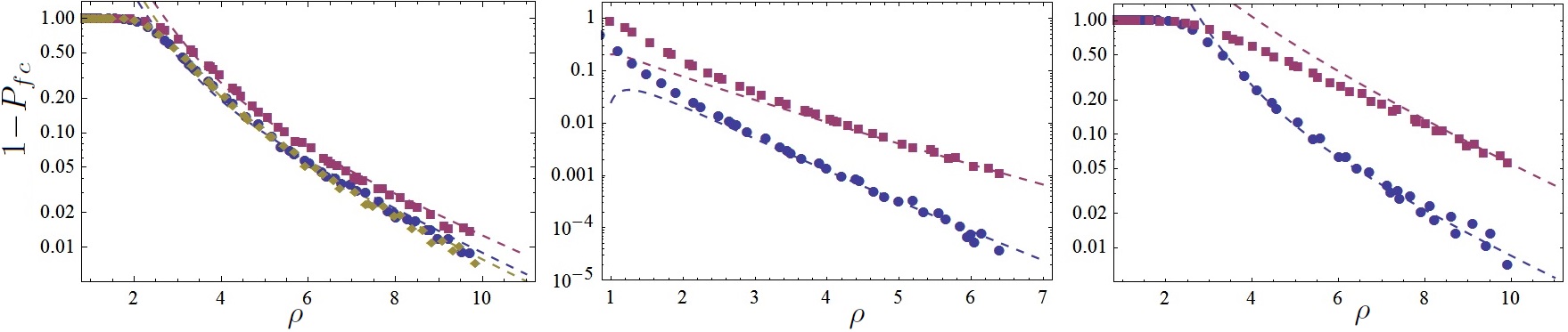
Figure 6: Full connection probability for a right triangle (side lengths 20 and 15) Left: Rayleigh with $\eta=3$ (top), $\eta=2$ (lower dark) and Rician with $\eta=2,K=4$ (lower light). Centre: MIMO with $\eta=3$ (top) and $\eta=2$ (bottom). Right: Soft annulus $r_{-}=1,r_{+}=2,a=1/3$ (top) and hard disk $r_{0}=1$ (bottom).

VII Conclusion

For random geometric graphs in finite geometries, the probability of (full) connection $P_{fc}$ can be conveniently approximated at high but finite node densities as a sum of separable boundary contributions. Showing that these contributions can be obtained from a few moments for a very general class of connection functions and geometries, thus vastly simplifying the evaluation of the relevant multidimensional integrals and hence the evaluation and design of ad-hoc wireless networks is the main contribution of the current paper. The results are in agreement with previous work and with numerics.

A number of previous works considered some examples where the above model and/or geometrical assumptions were relaxed, but not to the level of generality considered here:

• Dimensions other than $2$ or $3$: Eq. (80) suggests further generalisation of the formulas and approach to $d>3$ might be possible (though perhaps with fewer practical applications). On the other hand, for $d=1$ the connection probability is not dominated by that of an isolated node; it is quite likely in many parameter regimes for the network to split into two or more large pieces. For the unit disk model it is rather straightforward to calculate the probability of a gap of given size, but for soft connection functions it remains open.

• Anisotropic connections: These are of particular relevance in three dimensions (where antenna patterns are never exactly isotropic), and where beamforming is desirable to mitigate interference from other nodes. The link pairwise connection probability depends on orientation as well as mutual distance; see Refs. Coon and Dettmann (2013); Georgiou et al. (2013a).

• Non-smooth boundaries: Ref. Coon et al. (2014) considered a conical corner, which is not within the scope of the calculations presented in Sec. V. See also “non-convex” below.

• Non-convex domains with a line-of-sight (LOS) condition: Examples have included keyhole geometries with Georgiou et al. (2015) or without Georgiou et al. (2013c) reflections, circular or spherical obstacles Giles et al. (to be published) and fractal domains Dettmann et al. (to be published). In the latter, remarkably, it is found that $P_{fc}$ decreases toward zero in the limit of high density.

It would be interesting to extend the theory presented here to include these cases as well, providing a practical framework for understanding connectivity in diverse spatial networks.

References

• Gilbert (1961) E. N. Gilbert, J. Soc. Indust. Appl. Math. 9, 533 (1961).
• Barthélemy (2011) M. Barthélemy, Physics Reports 499, 1 (2011).
• Donges et al. (2009) J. F. Donges, Y. Zou, N. Marwan, and J. Kurths, The European Physical Journal Special Topics 174, 157 (2009).
• Robson et al. (2015) C. Robson, S. Barr, P. James, and A. Ford (2015).
• Blanchard and Volchenkov (2008) P. Blanchard and D. Volchenkov, Mathematical analysis of urban spatial networks (Springer Science & Business Media, 2008).
• Bullmore and Sporns (2012) E. Bullmore and O. Sporns, Nature Reviews Neuroscience 13, 336 (2012).
• Nicosia et al. (2013) V. Nicosia, P. E. Vértes, W. R. Schafer, V. Latora, and E. T. Bullmore, Proceedings of the National Academy of Sciences 110, 7880 (2013).
• Higham et al. (2008) D. J. Higham, M. Rašajski, and N. Pržulj, Bioinformatics 24, 1093 (2008).
• Haenggi et al. (2009) M. Haenggi, J. G. Andrews, F. Baccelli, O. Dousse, and M. Franceschetti, IEEE J. Select. Areas Comm. 27, 1029 (2009).
• Sarkar and Haenggi (2013) A. Sarkar and M. Haenggi, Discrete Applied Mathematics 161, 2120 (2013).
• Diaz-Guilera et al. (2009) A. Diaz-Guilera, J. Gómez-Gardenes, Y. Moreno, and M. Nekovee, International Journal of Bifurcation and Chaos 19, 687 (2009).
• Franceschetti et al. (2007) M. Franceschetti, O. Dousse, D. N. Tse, and P. Thiran, Information Theory, IEEE Transactions on 53, 1009 (2007).
• de Morais Cordeiro and Agrawal (2011) C. de Morais Cordeiro and D. P. Agrawal, Ad hoc and sensor networks: theory and applications (World Scientific, 2011).
• Walters (2011) M. Walters, Surveys in Combinatorics 392, 365 (2011).
• Mao and Anderson (2012) G. Mao and B. Anderson, IEEE/ACM Transactions on Networking (TON) 20, 408 (2012).
• Coon et al. (2012a) J. Coon, C. P. Dettmann, and O. Georgiou, J. Stat. Phys. 147, 758 (2012a).
• Mao and Anderson (2013) G. Mao and B. D. Anderson, Information Theory, IEEE Transactions on 59, 1761 (2013).
• Mao and Do Anderson (2014) G. Mao and B. Do Anderson, Wireless Communications, IEEE transactions on 13, 1678 (2014).
• Penrose (to be published) M. D. Penrose, arXiv:1311.3897; Ann. Appl. Prob. (to be published).
• Georgiou et al. (2014) O. Georgiou, C. P. Dettmann, and J. P. Coon, in IEEE ICC 2014 (2014), pp. 77–82.
• Coon et al. (2012b) J. Coon, C. P. Dettmann, and O. Georgiou, Phys. Rev. E 85, 011138 (2012b).
• Coon and Dettmann (2013) J. P. Coon and C. P. Dettmann, IEEE Comm. Lett. 17, 321 (2013).
• Georgiou et al. (2013a) O. Georgiou, C. P. Dettmann, and J. P. Coon, IEEE Trans. Wireless. Comm. 13, 4534 (2013a).
• Georgiou et al. (2013b) O. Georgiou, C. P. Dettmann, and J. P. Coon, EPL 103, 28006 (2013b).
• Georgiou et al. (2015) O. Georgiou, M. Z. Bocus, C. P. Dettmann, J. P. Coon, and M. R. Rahman, IEEE Commun. Lett. 19, 427 (2015).
• Georgiou et al. (2013c) O. Georgiou, C. P. Dettmann, and J. P. Coon, in Proc. ISWCS 2013 (VDE, 2013c), pp. 1–5.
• (27) M. D. Penrose, arxiv:1507.07132.
• Nuttall (1972) A. H. Nuttall, Tech. Rep., DTIC Document (1972).
• Simon (2002) M. K. Simon, Communications, IEEE Transactions on 50, 1712 (2002).
• Balister et al. (2004) P. Balister, B. Bollobás, and M. Walters, Annals of Applied Probability pp. 1869–1879 (2004).
• Kuhn et al. (2003) F. Kuhn, R. Wattenhofer, and A. Zollinger, in Proceedings of the 2003 joint workshop on Foundations of mobile computing (ACM, 2003), pp. 69–78.
• Gao et al. (2011) D. Gao, P. Chen, C. H. Foh, and Y. Niu, EURASIP Journal on Wireless Communications and Networking 2011, 1 (2011).
• Iyer et al. (2009) A. Iyer, C. Rosenberg, and A. Karnik, Wireless Communications, IEEE Transactions on 8, 2662 (2009).
• Durgin et al. (2002) G. D. Durgin, T. S. Rappaport, and D. A. De Wolf, IEEE Transactions on Communications 50, 1005 (2002).
• Coon et al. (2014) J. P. Coon, O. Georgiou, and C. P. Dettmann, in Proceedings of SPASWIN 2014: International workshop on spatial stochastic models for wireless networks (2014).
• Kang and Alouini (2003) M. Kang and M.-S. Alouini, Selected Areas in Communications, IEEE Journal on 21, 418 (2003).
• Alouini and Goldsmith (2000) M.-S. Alouini and A. J. Goldsmith, Wireless Personal Communications 13, 119 (2000).
• Alouini and Simon (2002) M.-S. Alouini and M. K. Simon, Communications, IEEE Transactions on 50, 1946 (2002).
• Erceg et al. (1999) V. Erceg, L. J. Greenstein, S. Y. Tjandra, S. R. Parkoff, A. Gupta, B. Kulic, A. A. Julius, and R. Bianchi, Selected Areas in Communications, IEEE Journal on 17, 1205 (1999).
• Waxman (1988) B. M. Waxman, Selected Areas in Communications, IEEE Journal on 6, 1617 (1988).
• Zegura et al. (1996) E. W. Zegura, K. L. Calvert, and S. B. Acharjee, in INFOCOM’96. Fifteenth Annual Joint Conference of the IEEE Computer Societies. Networking the Next Generation. Proceedings IEEE (IEEE, 1996), vol. 2, pp. 594–602.
• Giles et al. (to be published) A. Giles, O. Georgiou, and C. P. Dettmann, arXiv:1502.05440; J. Stat. Phys. (to be published).
• Dettmann et al. (to be published) C. P. Dettmann, O. Georgiou, and J. P. Coon, arXiv:1409.7520; Proc. IEEE ISWCS 2015 (to be published).