Singular foliations for M-theory compactification

Abstract

We use the theory of singular foliations to study $\mathcal{N}=1$ compactifications of eleven-dimensional supergravity on eight-manifolds $M$ down to $\mathrm{AdS}_{3}$ spaces, allowing for the possibility that the internal part $\xi$ of the supersymmetry generator is chiral on some locus $\mathcal{W}$ which does not coincide with $M$. We show that the complement $M\setminus\mathcal{W}$ must be a dense open subset of $M$ and that $M$ admits a singular foliation ${\bar{\mathcal{F}}}$ endowed with a longitudinal $G_{2}$ structure and defined by a closed one-form ${\boldsymbol{\omega}}$, whose geometry is determined by the supersymmetry conditions. The singular leaves are those leaves which meet $\mathcal{W}$. When ${\boldsymbol{\omega}}$ is a Morse form, the chiral locus is a finite set of points, consisting of isolated zero-dimensional leaves and of conical singularities of seven-dimensional leaves. In that case, we describe the topology of $\bar{\mathcal{F}}$ using results from Novikov theory. We also show how this description fits in with previous formulas which were extracted by exploiting the $\mathrm{Spin}(7)_{\pm}$ structures which exist on the complement of $\mathcal{W}$.

Introduction

$\mathcal{N}=1$ flux compactifications of eleven-dimensional supergravity on eight-manifolds $M$ down to $\mathrm{AdS}_{3}$ spaces MartelliSparks ; Tsimpis provide a vast extension of the better studied class of compactifications down to 3-dimensional Minkowski space Becker1 ; Becker2 ; Constantin , having the advantage that they are already consistent at the classical level MartelliSparks . They form a useful testing ground for various proposals aimed at providing unified descriptions of flux backgrounds Grana and may be relevant to recent attempts to gain a better understanding of F-theory Bonetti . When the internal part $\xi$ of the supersymmetry generator is everywhere non-chiral, such backgrounds can be studied g2 using foliations endowed with longitudinal $G_{2}$ structures, an approach which permits a geometric description of the supersymmetry conditions while providing powerful tools for studying the topology of such backgrounds.

In this paper, we extend the results of g2 to the general case when the internal part $\xi$ of the supersymmetry generator is allowed to become chiral on some locus $\mathcal{W}\subset M$. Assuming that $\mathcal{W}\neq M$, i.e. that $\xi$ is not everywhere chiral, we show that, at the classical level, the Einstein equations imply that the chiral locus $\mathcal{W}$ must be a set with empty interior, which therefore is negligible with respect to the Lebesgue measure of the internal space. As a consequence, the behavior of geometric data along this locus can be obtained from the non-chiral locus $\mathcal{U}\stackrel{{\scriptstyle{\rm def.}}}{{=}}M\setminus\mathcal{W}$ through a limiting process. The geometric information along the non-chiral locus $\mathcal{U}$ is encoded g2 by a regular foliation $\mathcal{F}$ which carries a longitudinal $G_{2}$ structure and whose geometry is determined by the supersymmetry conditions in terms of the supergravity four-form field strength. When $\emptyset\neq\mathcal{W}\subsetneq M$, we show that $\mathcal{F}$ extends to a singular foliation $\bar{\mathcal{F}}$ of the whole manifold $M$ by adding leaves which are allowed to have singularities at points belonging to $\mathcal{W}$. This singular foliation “integrates” a cosmooth BulloLewis ; Drager ; Michor ; Ratiu singular distribution $\mathcal{D}$ (a.k.a. generalized sub-bundle of $TM$), defined as the kernel distribution of a closed one-form ${\boldsymbol{\omega}}$ which belongs to a cohomology class $\mathfrak{f}\in H^{1}(M,\mathbb{R})$ determined by the supergravity four-form field strength. The set of zeroes of ${\boldsymbol{\omega}}$ coincides with the chiral locus $\mathcal{W}$. In the most general case, $\bar{\mathcal{F}}$ can be viewed as a Haefliger structure Haefliger on $M$. The singular foliation $\bar{\mathcal{F}}$ carries a longitudinal $G_{2}$ structure, which is allowed to degenerate at the singular points of singular leaves. On the non-chiral locus $\mathcal{U}$, the problem can be studied using the approach of g2 or the approach advocated in Tsimpis , which makes use of two $\mathrm{Spin}(7)_{\pm}$ structures. We show explicitly how one can translate between these two approaches and prove that the results of g2 agree with those of Tsimpis along this locus.

While the topology of singular foliations defined by a closed one-form can be extremely complicated in general, the situation is better understood in the case when ${\boldsymbol{\omega}}$ is a Morse one-form. The Morse case is generic in the sense that such 1-forms constitute an open and dense subset of the set of all closed one-forms belonging to the cohomology class $\mathfrak{f}$. In the Morse case, the singular foliation $\bar{\mathcal{F}}$ can be described using the foliation graph MelnikovaThesis ; MelnikovaGraph ; FKL associated to the corresponding decomposition of $M$ (see Melnikova2 ; Melnikova3 ; FKL and Gelbukh1 –Gelbukh9 ), which provides a combinatorial way to encode some important aspects of the foliation’s topology — up to neglecting the information contained in the so-called minimal components of the decomposition, components which should possess an as yet unexplored non-commutative geometric description. This provides a far-reaching extension of the picture found in g2 for the everywhere non-chiral case $\mathcal{U}=M$, a case which corresponds to the situation when the foliation graph is reduced to either a circle (when $\mathcal{F}$ has compact leaves, being a fibration over $S^{1}$) or to a single so-called exceptional vertex (when $\mathcal{F}$ has non-compact dense leaves, being a minimal foliation). In the minimal case of the backgrounds considered g2 , the exceptional vertex corresponds to a noncommutative torus which encodes the noncommutative geometry ConnesFol ; ConnesNG of the leaf space.

The paper is organized as follows. Section 1 gives a brief review of the class of compactifications we consider, in order to fix notations and conventions. Section 2 discusses a geometric characterization of Majorana spinors $\xi$ on $M$ which is inspired by the rigorous approach developed in ga1 ; ga2 ; gf for the method of bilinears Tod , in the case when the spinor $\xi$ is allowed to be chiral at some loci. It also gives the Kähler-Atiyah parameterizations of this spinor which correspond to the approach of g2 and to that of Tsimpis and describes the relevant $G$-structures using both spinors and idempotents in the Kähler-Atiyah algebra of $M$. In the same section, we give the general description of the singular foliation $\bar{\mathcal{F}}$ as the Haefliger structure defined by the closed one-form ${\boldsymbol{\omega}}$. Section 3 describes the relation between the $G_{2}$ and $\mathrm{Spin}(7)_{\pm}$ parameterizations of the fluxes as well as the relation between the torsion classes of the leafwise $G_{2}$ structure and the Lee form and characteristic torsion of the $\mathrm{Spin}(7)_{\pm}$ structures defined on the non-chiral locus. The same section gives the comparison of the approach of g2 with that of Tsimpis along that locus. Section 4 discusses the topology of the singular foliation $\bar{\mathcal{F}}$ in the Morse case while Section 5 concludes. The appendices contain various technical details.

Notations and conventions.

Throughout this paper, $M$ denotes an oriented, connected and compact smooth manifold (which will mostly be of dimension eight), whose unital commutative $\mathbb{R}$-algebra of smooth real-valued functions we denote by $\Omega^{0}(M)={{\cal\mathcal{C}}^{\infty}(M,\mathbb{R})}$. Given a subset $A$ of $M$, we let ${\bar{A}}$ denote the closure of $A$ in $M$ (taken with respect to the manifold topology of $M$). The large topological frontier (also called topological boundary) of $A$ is defined as $\mathrm{Fr}(A)\stackrel{{\scriptstyle{\rm def.}}}{{=}}{\bar{A}}\setminus\mathrm{Int}(A)$, where $\mathrm{Int}(A)$ denotes the interior of $A$. The small topological frontier is $\mathrm{fr}(A)\stackrel{{\scriptstyle{\rm def.}}}{{=}}{\bar{A}}\setminus A$. Notice that $\mathrm{fr}(A)\subseteq\mathrm{Fr}(A)$ and that $\mathrm{fr}(A)=\mathrm{Fr}(A)$ when $A$ is open, in which case we speak simply of the frontier of $A$. All fiber bundles we consider are smooth. We use freely the results and notations of ga1 ; ga2 ; gf ; g2 , with the same conventions as there. To simplify notation, we write the geometric product $\diamond$ of ga1 ; ga2 ; gf simply as juxtaposition while indicating the wedge product of differential forms through $\wedge$. If $\mathcal{D}\subset TM$ is a singular (a.k.a. generalized) distribution on $M$ and $\mathcal{U}$ is an open subset of $M$ such that $\mathcal{D}|_{\mathcal{U}}$ is a regular Frobenius distribution (see Appendix D), we let $\Omega_{\mathcal{U}}(\mathcal{D})=\Gamma(\mathcal{U},\wedge(\mathcal{D}|_{\mathcal{U}})^{\ast})$ denote the $\mathcal{C}^{\infty}(\mathcal{U},\mathbb{R})$-module of $\mathcal{D}|_{\mathcal{U}}$-longitudinal differential forms defined on $\mathcal{U}$. When $\dim M=8$, then for any 4-form $\omega\in\Omega^{4}(M)$ we let $\omega^{\pm}\stackrel{{\scriptstyle{\rm def.}}}{{=}}\frac{1}{2}(\omega\pm\ast\omega)$ denote the selfdual and anti-selfdual parts of $\omega$ (namely, $\ast\omega^{\pm}=\pm\omega^{\pm}$). When $M$ is eight-dimensional, we let $\Omega^{4\pm}(M)$ denote the spaces of selfdual and anti-selfdual four-forms, respectively. We use the “Det” convention for the wedge product and the corresponding “Perm” convention for the symmetric product. Hence given a local coframe $e^{a}$ of $M$, we have:

$$\begin{split}&e^{a_{1}}\wedge\ldots\wedge e^{a_{k}}\stackrel{{\scriptstyle{\rm def.}}}{{=}}\sum_{\sigma\in S_{k}}\epsilon(\sigma)e^{a_{\sigma(1)}}\otimes\ldots\otimes e^{a_{\sigma(k)}}~{}~{},\\ &e^{a_{1}}\odot\ldots\odot e^{a_{k}}\stackrel{{\scriptstyle{\rm def.}}}{{=}}\sum_{\sigma\in S_{k}}e^{a_{\sigma(1)}}\otimes\ldots\otimes e^{a_{\sigma(k)}}~{}~{},\end{split}$$ (1)

without prefactors of $\frac{1}{k!}$ in the right hand side, where $S_{k}$ is the symmetric group on $k$ letters and $\epsilon(\sigma)$ denotes the signature of a permutation $\sigma$. This is the convention used, for example, in Spivak . We use $\mathrm{Sym}^{2}_{0}(T^{\ast}M)$ to denote the space of traceless symmetric covariant 2-tensors on $M$ and $\mathrm{Sym}^{2}_{\mathcal{U},0}(\mathcal{D}^{\ast})$ to denote the space of traceless symmetric covariant 2-tensors defined on $\mathcal{U}$ and which are longitudinal to the Frobenius distribution $\mathcal{D}|_{\mathcal{U}}$, when $\mathcal{D}$ is as above. By definition, a $\mathrm{Spin}(7)_{+}$ structure on $M$ is a $\mathrm{Spin}(7)$ structure with respect to the orientation chosen for $M$ while a $\mathrm{Spin}(7)_{-}$ structure is a $\mathrm{Spin}(7)$ structure with respect to the opposite orientation.

1 Basics

We start with a brief review of the set-up, in order to fix notation. As in MartelliSparks ; Tsimpis , we consider 11-dimensional supergravity sugra11 on an eleven-dimensional connected and paracompact spin manifold $\mathbf{M}$ with Lorentzian metric $\mathbf{g}$ (of ‘mostly plus’ signature). Besides the metric, the classical action of the theory contains the three-form potential with four-form field strength $\mathbf{G}\in\Omega^{4}(\mathbf{M})$ and the gravitino $\mathbf{\Psi}$, which is a Majorana spinor of spin $3/2$. The bosonic part of the action takes the form:

$$S_{\rm bos}[\mathbf{g},\mathbf{C}]=\frac{1}{2\mathbf{\kappa}_{11}^{2}}\int_{\mathbf{M}}R\boldsymbol{\nu}-\frac{1}{4\mathbf{\kappa}_{11}^{2}}\int_{\mathbf{M}}\big{(}\mathbf{G}\wedge\star\mathbf{G}+\frac{1}{3}\mathbf{C}\wedge\mathbf{G}\wedge\mathbf{G}\big{)}~{}~{},$$

where $\mathbf{\kappa}_{11}$ is the gravitational coupling constant in eleven dimensions, $\boldsymbol{\nu}$ and $R$ are the volume form and the scalar curvature of $\mathbf{g}$ and $\mathbf{G}=\mathrm{d}\mathbf{C}$. For supersymmetric bosonic classical backgrounds, both the gravitino and its supersymmetry variation must vanish, which requires that there exist at least one solution $\boldsymbol{\eta}$ to the equation:

$$\delta_{\boldsymbol{\eta}}\mathbf{\Psi}\stackrel{{\scriptstyle{\rm def.}}}{{=}}\mathfrak{D}\boldsymbol{\eta}=0~{}~{},$$ (2)

where $\mathfrak{D}$ denotes the supercovariant connection. The eleven-dimensional supersymmetry generator $\boldsymbol{\eta}$ is a Majorana spinor (real pinor) of spin $1/2$ on $\mathbf{M}$.

As in MartelliSparks ; Tsimpis , consider compactification down to an $\mathrm{AdS}_{3}$ space of cosmological constant $\Lambda=-8\kappa^{2}$, where $\kappa$ is a positive real parameter — this includes the Minkowski case as the limit $\kappa\rightarrow 0$. Thus $\mathbf{M}=N\times M$, where $N$ is an oriented 3-manifold diffeomorphic to $\mathbb{R}^{3}$ and carrying the $\mathrm{AdS}_{3}$ metric $g_{3}$ while $M$ is an oriented, compact and connected Riemannian eight-manifold whose metric we denote by $g$. The metric on $\mathbf{M}$ is a warped product:

$$\mathrm{d}\mathbf{s}^{2} = e^{2\Delta}\mathrm{d}s^{2}~{}~{}~{}{\rm where}~{}~{}~{}\mathrm{d}s^{2}=\mathrm{d}s^{2}_{3}+g_{mn}\mathrm{d}x^{m}\mathrm{d}x^{n}~{}~{}.$$ (3)

The warp factor $\Delta$ is a smooth real-valued function defined on $M$ while $\mathrm{d}s_{3}^{2}$ is the squared length element of the $\mathrm{AdS}_{3}$ metric $g_{3}$. For the field strength $\mathbf{G}$, we use the ansatz:

$$\mathbf{G}=\nu_{3}\wedge\mathbf{f}+\mathbf{F}~{}~{},~{}~{}~{}~{}\mathrm{with}~{}~{}\mathbf{F}\stackrel{{\scriptstyle{\rm def.}}}{{=}}e^{3\Delta}F~{}~{},~{}~{}\mathbf{f}\stackrel{{\scriptstyle{\rm def.}}}{{=}}e^{3\Delta}f~{}~{},$$ (4)

where $f\in\Omega^{1}(M)$, $F\in\Omega^{4}(M)$ and $\nu_{3}$ is the volume form of $(N,g_{3})$. For $\boldsymbol{\eta}$, we use the ansatz:

$$\boldsymbol{\eta}=e^{\frac{\Delta}{2}}(\zeta\otimes\xi)~{}~{},$$

where $\xi$ is a Majorana spinor of spin $1/2$ on the internal space $(M,g)$ (a section of the rank 16 real vector bundle $S$ of indefinite chirality real pinors) and $\zeta$ is a Majorana spinor on $(N,g_{3})$.

Assuming that $\zeta$ is a Killing spinor on the $\mathrm{AdS}_{3}$ space $(N,g_{3})$, the supersymmetry condition (2) is equivalent with the following system for $\xi$:

$$\boxed{\mathbb{D}\xi=0~{}~{},~{}~{}Q\xi=0}~{}~{},$$ (5)

where

$$\mathbb{D}_{X}=\nabla_{X}^{S}+\frac{1}{4}\gamma(X\lrcorner F)+\frac{1}{4}\gamma((X_{\sharp}\wedge f)\nu)+\kappa\gamma(X\lrcorner\nu)~{}~{},~{}~{}X\in\Gamma(M,TM)$$

is a linear connection on $S$ (here $\nabla^{S}$ is the connection induced on $S$ by the Levi-Civita connection of $(M,g)$, while $\nu$ is the volume form of $(M,g)$) and

$$Q=\frac{1}{2}\gamma(\mathrm{d}\Delta)-\frac{1}{6}\gamma(\iota_{f}\nu)-\frac{1}{12}\gamma(F)-\kappa\gamma(\nu)$$

is a globally-defined endomorphism of $S$. As in MartelliSparks ; Tsimpis , we do not require that $\xi$ has definite chirality.

The set of solutions of (5) is a finite-dimensional $\mathbb{R}$-linear subspace $\mathrm{\cal K}(\mathbb{D},{Q})$ of the infinite-dimensional vector space $\Gamma(M,S)$ of smooth sections of $S$. Up to rescalings by smooth nowhere-vanishing real-valued functions defined on $M$, the vector bundle $S$ has two admissible pairings $\Scr B_{\pm}$ (see gf ; AC1 ; AC2 ), both of which are symmetric but which are distinguished by their types $\epsilon_{\Scr B_{\pm}}=\pm 1$. Without loss of generality, we choose to work with $\Scr B\stackrel{{\scriptstyle{\rm def.}}}{{=}}\Scr B_{+}$. We can in fact take $\Scr B$ to be a scalar product on $S$ and denote the corresponding norm by $||~{}||$ (see ga1 ; ga2 for details). Requiring that the background preserves exactly $\mathcal{N}=1$ supersymmetry amounts to asking that $\dim\mathrm{\cal K}(\mathbb{D},Q)=1$. It is not hard to check ga1 that $\Scr B$ is $\mathbb{D}$-flat:

$$\mathrm{d}\Scr B(\xi^{\prime},\xi^{\prime\prime})=\Scr B(\mathbb{D}\xi^{\prime},\xi^{\prime\prime})+\Scr B(\xi^{\prime},\mathbb{D}\xi^{\prime\prime})~{}~{},~{}~{}\forall\xi^{\prime},\xi^{\prime\prime}\in\Gamma(M,S)~{}~{}.$$ (6)

Hence any solution of (5) which has unit $\Scr B$-norm at a point will have unit $\Scr B$-norm at every point of $M$ and we can take the internal part $\xi$ of the supersymmetry generator to be everywhere of norm one.

2 Parameterizing a Majorana spinor on $M$

2.1 Globally valid parameterization

Fixing a Majorana spinor $\xi\in\Gamma(M,S)$ which is everywhere of $\Scr B$-norm one, consider the inhomogeneus differential form:

$$\check{E}_{\xi,\xi}=\frac{1}{16}\sum_{k=0}^{8}\boldsymbol{\check{E}}^{(k)}_{\xi,\xi}\in\Omega(M)~{}~{},$$ (7)

whose rescaled rank components have the following expansions in any local orthonormal coframe $(e^{a})_{a=1\ldots 8}$ of $M$ defined on some open subset $U$:

$$\boldsymbol{\check{E}}^{(k)}_{\xi,\xi}=_{U}\frac{1}{k!}\Scr B(\xi,\gamma_{a_{1}...a_{k}}\xi)e^{a_{1}...a_{k}}\in\Omega^{k}(M)~{}~{}.$$

The conditions:

$$\check{E}^{2}=\check{E}~{}~{},~{}~{}~{}\mathcal{S}(\check{E})=1~{}~{},~{}~{}\tau(\check{E})=\check{E}~{}~{}$$ (8)

encode the fact that an inhomogeneous form $\check{E}\stackrel{{\scriptstyle{\rm def.}}}{{=}}\check{E}_{\xi,\xi}$ is of the type (7) for some Majorana spinor $\xi$ which is everywhere of norm one. As a result of the last condition in (8), the non-zero components of $\check{E}$ have ranks $k=0,1,4,5$ and we have $\mathcal{S}(\check{E}_{\xi,\xi})=\boldsymbol{\check{E}}^{(0)}_{\xi,\xi}=||\xi||^{2}=1$, where $\mathcal{S}$ is the canonical trace of the Kähler-Atiyah algebra. Hence:

$$\boxed{\check{E}=\frac{1}{16}(1+V+Y+Z+b\nu)}~{}~{},$$ (9)

where we introduced the notations:

$$V\stackrel{{\scriptstyle{\rm def.}}}{{=}}\boldsymbol{\check{E}}^{(1)}~{}~{},~{}~{}Y\stackrel{{\scriptstyle{\rm def.}}}{{=}}\boldsymbol{\check{E}}^{(4)}~{},~{}~{}Z\stackrel{{\scriptstyle{\rm def.}}}{{=}}\boldsymbol{\check{E}}^{(5)}~{}~{},~{}~{}b\nu\stackrel{{\scriptstyle{\rm def.}}}{{=}}\boldsymbol{\check{E}}^{(8)}~{}~{}.$$ (10)

Here, $b$ is a smooth real valued function defined on $M$ and $\nu$ is the volume form of $(M,g)$, which satisfies $||\nu||=1$; notice the relation $\mathcal{S}(\nu\check{E}_{\xi,\xi})=b$. On a small enough open subset $U\subset M$ supporting a local coframe $(e^{a})$ of $M$, one has the expansions:

$$V=_{U}\Scr B(\xi,\gamma_{a}\xi)e^{a}~{}~{},~{}~{}Y=_{U}\frac{1}{4!}\Scr B(\xi,\gamma_{a_{1}\ldots a_{4}}\xi)e^{a_{1}\ldots a_{4}}~{},$$

$$Z=_{U}\frac{1}{5!}\Scr B(\xi,\gamma_{a_{1}\ldots a_{5}}\xi)e^{a_{1}\ldots a_{5}}~{}~{},~{}~{}b=_{U}\Scr B(\xi,\gamma(\nu)\xi)~{}~{}.$$ (11)

One finds ga1 that (8) is equivalent with the following relations which hold globally on $M$:

$$\boxed{\begin{split}&||V||^{2}=1-b^{2}\geq 0~{}~{},~{}~{}||Y^{\pm}||^{2}=\frac{7}{2}(1\pm b)^{2}~{}~{},\\ &\iota_{V}(\ast Z)=0~{}~{},~{}~{}\iota_{V}Z=Y-b\ast Y~{}~{},\\ &(\iota_{\alpha}(\ast Z))\wedge(\iota_{\beta}(\ast Z))\wedge(\ast Z)=-6\langle\alpha\wedge V,\beta\wedge V\rangle\iota_{V}\nu~{}~{},~{}~{}\forall\alpha,\beta\in\Omega^{1}(M)~{}~{}.\end{split}}$$ (12)

Notice that the first relation in the second row is equivalent with $V\wedge Z=0$, which means that $V$ and $Z$ commute in the Kähler-Atiyah algebra of $(M,g)$.

Remark.

Let (R) denote the second relation (namely $\iota_{V}Z=Y-b\ast Y$) on the second row of (12). Separating the selfdual and anti-selfdual parts shows that (R) is equivalent with the following two conditions:

$$(\iota_{V}Z)^{\pm}=(1\mp b)Y^{\pm}~{}~{}.$$ (13)

Proposition.

Relations (12) imply that the following normalization conditions hold globally on $M$:

$$||Y||^{2}=7(1+b^{2})~{}~{},~{}~{}||Z||^{2}=7(1-b^{2})~{}~{}.$$ (14)

Proof. The first equation in (14) follows from the last relations on the first row of (12) by noticing that $||Y||^{2}=||Y^{+}||^{2}+||Y^{-}||^{2}$ (since $\langle Y^{+},Y^{-}\rangle=0$). We have:

$$||\iota_{V}Z||^{2}=||\ast\iota_{V}Z||^{2}=||V\wedge(\ast Z)||^{2}=||V||^{2}||\ast Z||^{2}=||V||^{2}||Z||^{2}~{}~{},$$ (15)

where in the middle equality we used the first equation on the second row of (12), which tells us that $\ast Z$ is orthogonal on $V$. The second equation in (14) now follows from (15) and from the identity:

$$||\iota_{V}Z||^{2}=(1-b)^{2}||Y^{+}||^{2}+(1+b)^{2}||Y^{-}||^{2}=7(1-b^{2})=7||V||^{2}~{}~{},$$

where we used (13) and both relations in the first row of (12). $\blacksquare$

The twisted selfdual and twisted anti-selfdual parts of $\check{E}$.

The identity $\nu^{2}=1$ implies that the elements:

$$R^{\pm}\stackrel{{\scriptstyle{\rm def.}}}{{=}}\frac{1}{2}(1\pm\nu)~{}~{}$$

are complementary idempotents in the Kähler-Atiyah algebra:

$$(R^{\pm})^{2}=R^{\pm}~{}~{},~{}~{}R^{\pm}R^{\mp}=0~{}~{},~{}~{}R^{+}+R^{-}=\mathrm{id}_{\Omega(M)}~{}~{}.$$ (16)

The (anti)selfdual part of a four-form $\omega\in\Omega^{4}(M)$ can be expressed as:

$$\omega_{\pm}=R^{\pm}\omega~{}~{}.$$

Notice that this relation also gives the twisted (anti)selfdual parts ga1 of an inhomogeneous form $\omega\in\Omega(M)$. The identities:

$$YR^{\pm}=R^{\pm}Y=Y^{\pm}~{}~{},~{}~{}(1+b\nu)R^{\pm}=(1\pm b)R^{\pm}~{}~{}$$

allow us to compute the twisted selfdual part $\check{E}^{+}$ and twisted anti-selfdual part $\check{E}^{-}$ of $\check{E}$:

$$\check{E}^{\pm}=\check{E}R^{\pm}=\frac{1}{16}\left[(1\pm b+V+Z)R_{\pm}+Y^{\pm}\right]\in\Omega(M)~{}~{}.$$ (17)

The following decomposition holds globally on $M$:

$$\check{E}=\check{E}^{+}+\check{E}^{-}~{}~{}.$$

2.2 The chirality decomposition of $M$

Let $S^{\pm}\subset S$ be the rank eight subbundles of $S$ consisting of positive and negative chirality spinors (the eigen-subbundles of $\gamma(\nu)$ corresponding to the eigenvalues $+1$ and $-1$). Since $\gamma(\nu)$ is $\Scr B$-symmetric, $S^{+}$ and $S^{-}$ give a $\Scr B$-orthogonal decomposition $S=S^{+}\oplus S^{-}$. Decomposing a normalized spinor as $\xi=\xi^{+}+\xi^{-}$ with $\xi^{\pm}\stackrel{{\scriptstyle{\rm def.}}}{{=}}\frac{1}{2}(\mathrm{id}_{S}\pm\gamma(\nu))\xi\in\Gamma(M,S^{\pm})$, we have:

$$||\xi||^{2}=||\xi^{+}||^{2}+||\xi^{-}||^{2}=1$$

and:

$$b=\Scr B(\xi,\gamma(\nu)\xi)=||\xi^{+}||^{2}-||\xi^{-}||^{2}~{}~{}.$$

These two relations give:

$$\boxed{||\xi^{\pm}||^{2}=\frac{1}{2}(1\pm b)}~{}~{}.$$ (18)

Notice that $b$ equals $\pm 1$ at a point $p\in M$ iff $\xi_{p}\in S^{\pm}_{p}$. Since $||V||^{2}=1-b^{2}$, the one-form $V$ vanishes at $p$ iff $\xi_{p}$ is chiral i.e. iff $\xi_{p}\in S_{p}^{+}\cup S_{p}^{-}$. Consider the non-chiral locus (an open subset of $M$):

$$\mathcal{U}\stackrel{{\scriptstyle{\rm def.}}}{{=}}\{p\in M|\xi\not\in S_{p}^{+}\cup S_{p}^{-}\}=\{p\in M|\xi^{+}_{p}\neq 0~{}\mathrm{and}~{}~{}\xi_{p}^{-}\neq 0\}=\{p\in M|V_{p}\neq 0\}=\{p\in M||b(p)|<1\}~{}~{},$$

and its closed complement, the chiral locus:

$$\mathcal{W}\stackrel{{\scriptstyle{\rm def.}}}{{=}}M\setminus\mathcal{U}=\{p\in M|\xi_{p}\in S_{p}^{+}\cup S^{-}_{p}\}=\{p\in M|\xi^{+}_{p}=0~{}\mathrm{or}~{}\xi^{-}_{p}=0\}=\{p\in M|V_{p}=0\}=\{p\in M||b(p)|=1\}~{}~{}.$$

The chiral locus $\mathcal{W}$ decomposes further as a disjoint union of two closed subsets, the positive and negative chirality loci:

$$\mathcal{W}=\mathcal{W}^{+}\sqcup\mathcal{W}^{-}~{}~{},$$

where:

$$\mathcal{W}^{\pm}\stackrel{{\scriptstyle{\rm def.}}}{{=}}\{p\in M|\xi_{p}\in S^{\pm}_{p}\}=\{p\in M|b(p)=\pm 1\}=\{p\in M|\xi_{p}^{\mp}=0\}~{}~{}.$$

The extreme cases $\mathcal{W}^{+}=M$ or $\mathcal{W}^{-}=M$, as well as $\mathcal{W}^{+}=\mathcal{W}^{-}=\emptyset$ are allowed. However, the case $\mathcal{U}=\emptyset$ with both $\mathcal{W}^{+}$ and $\mathcal{W}^{-}$ nonempty (then $M=\mathcal{W}^{+}\sqcup\mathcal{W}^{-}$) is forbidden (recall that $b$ is smooth and hence continuous while $M$ is connected). Since $\xi$ does not vanish on $M$, we have:

$$\mathcal{U}^{\pm}\stackrel{{\scriptstyle{\rm def.}}}{{=}}\mathcal{U}\cup\mathcal{W}^{\pm}=\{p\in M|\xi^{\pm}_{p}\neq 0\}~{}~{}.$$

Remark.

Since $|b|\leq 1$ on $M$, the sets $\mathcal{W}^{\pm}$ (when non-empty) consist of critical points of $b$, namely the absolute maxima and minima of $b$ on $M$. Hence the differential of $b$ vanishes at every point of $\mathcal{W}$. In general $\mathcal{W}^{\pm}$ can be quite ‘wild’ (they can be very far from being immersed submanifolds of $M$).

2.3 A topological no-go theorem

Recall that $M$ is compact. The following result clarifies the kind of topologies of the chiral loci which are of physical interest.

Theorem

Assume that the supersymmetry conditions, the Bianchi identity and equations of motion for $G$ as well as the Einstein equations are satisfied. There exist only the following four possibilities:

1. The set $\mathcal{W}^{+}$ coincides with $M$ and hence $\mathcal{W}^{-}$ and $\mathcal{U}$ are empty. In this case, $\xi$ is a chiral spinor of positive chirality which is covariantly constant on $M$ and we have $\kappa=f=F=0$ while $\Delta$ is constant on $M$.

2. The set $\mathcal{W}^{-}$ coincides with $M$ and hence $\mathcal{W}^{+}$ and $\mathcal{U}$ are empty. In this case, $\xi$ is a chiral spinor of negative chirality which is covariantly constant on $M$ and we have $\kappa=f=F=0$ while $\Delta$ is constant on $M$.

3. The set $\mathcal{U}$ coincides with $M$ and hence $\mathcal{W}^{+}$ and $\mathcal{W}^{-}$ are empty.

4. At least one of the sets $\mathcal{W}^{+}$ or $\mathcal{W}^{-}$ is non-empty but both of these sets have empty interior. In this case, $\mathcal{U}$ is dense in $M$ and the union $\mathcal{W}=\mathcal{W}^{+}\cup\mathcal{W}^{-}$ coincides with the topological frontier $\mathrm{Fr}(\mathcal{U})=\mathrm{fr}(\mathcal{U})={\bar{\mathcal{U}}}\setminus\mathcal{U}$ of $\mathcal{U}$.

The proof of the theorem is given in Appendix A.

Remarks.

• The theorem is a strengthening of an observation originally made in MartelliSparks in the case when $\xi$ is nowhere-chiral.

• The theorem holds in classical supergravity only. One may be able to avoid its conclusions by considering quantum corrections.

• Cases 1 and 2 correspond to the classical limit of the compactifications studied in Becker1 ; Becker2 ; Constantin . Case 3 was studied in MartelliSparks ; g2 .

The study of Case 4 is the focus of the present paper. Due to the theorem, we shall from now on assume that we are in this case, i.e. that $\mathcal{W}$ is non-empty and that it coincides with the frontier of $\mathcal{U}$; in particular, we can assume that the closure of $\mathcal{U}$ coincides with $M$:

$$M={\bar{\mathcal{U}}}=\mathcal{U}\sqcup\mathcal{W}~{}~{},~{}~{}\mathcal{W}=\mathrm{Fr}\mathcal{U}~{}~{}.$$

In Figure 1, we sketch the chirality decomposition in two sub-cases of Case 4, which correspond to the assumptions that the one-form ${\boldsymbol{\omega}}\stackrel{{\scriptstyle{\rm def.}}}{{=}}4\kappa e^{3\Delta}V$ is of Morse and Bott-Morse type, respectively.

​​​​​

​​​​​

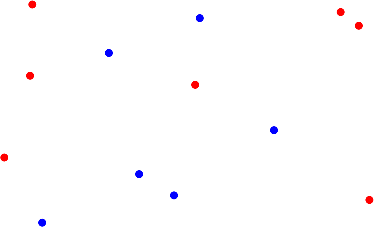
(a) Sketch of the chiral loci in the Morse sub-case of Case 4 of the Theorem. In this case, each of $\mathcal{W}^{+}$ and $\mathcal{W}^{-}$ is a finite set of points, with the points of $\mathcal{W}^{+}$ indicated in red and those of $\mathcal{W}^{-}$ indicated in blue.

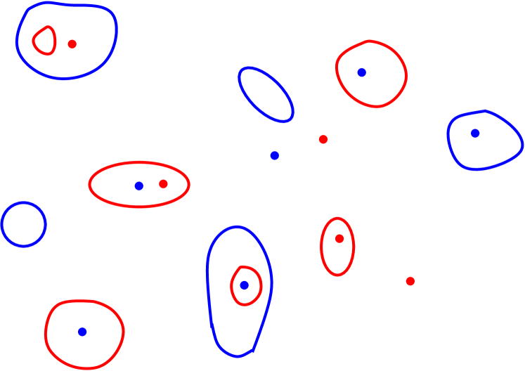
(b) Sketch of $\mathcal{W}^{\pm}$ in the Bott-Morse sub-case of Case 4 of the Theorem. The connected components of $\mathcal{W}$ are submanifolds of various dimensions, shown respectively in red and blue for $\mathcal{W}^{+}$ and $\mathcal{W}^{-}$.

Figure 1: Sketch of chiral loci in two sub-cases of Case 4 of the Theorem, for the case of a two-dimensional manifold $M$. The non-chiral locus $\mathcal{U}$ is the complement of $\mathcal{W}$ in $M$ and is indicated by white space, after performing appropriate cuts which allow one to map $M$ to some region of the plane which is not indicated explicitly. The figures should be interpreted with care in our case $\dim M=8$.

2.4 The singular distribution $\mathcal{D}$

The one-form $V$ determines a singular (a.k.a. generalized) distribution $\mathcal{D}$ (generalized sub-bundle of $TM$) which is defined through:

$$\mathcal{D}_{p}\stackrel{{\scriptstyle{\rm def.}}}{{=}}{\ker V_{p}}~{}~{},~{}~{}\forall p\in M~{}~{}.$$

This singular distribution is cosmooth (rather than smooth) in the sense of Drager (see Appendix D). Notice that $\mathcal{D}$ is smooth iff $\xi$ is everywhere non-chiral — i.e. iff $\mathcal{W}=\emptyset$, which is the case studied in g2 ; in that case, $\mathcal{D}$ is a regular Frobenius distribution. Since in this paper we assume $\mathcal{W}\neq\emptyset$, it follows that $\mathcal{D}$ is not a singular distribution in the sense of Stefan-Sussmann Stefan ; Sussmann . The set of regular points of $\mathcal{D}$ equals the non-chiral locus $\mathcal{U}$ and we have:

$${\rm rk}\mathcal{D}_{p} = 7~{}~{}\mathrm{when}~{}~{}p\in\mathcal{U}~{}~{},$$

$${\rm rk}\mathcal{D}_{p} = 8~{}~{}\mathrm{when}~{}~{}p\in\mathcal{W}~{}~{}.$$

In particular, the restriction $\mathcal{D}|_{\mathcal{U}}$ is a regular Frobenius distribution on the non-chiral locus $\mathcal{U}$. As in g2 , we endow $\mathcal{D}|_{\mathcal{U}}$ with the orientation induced by that of $M$ using the unit norm vector field $n\stackrel{{\scriptstyle{\rm def.}}}{{=}}{\hat{V}}^{\sharp}=\frac{1}{||V||}V^{\sharp}$, which corresponds to the $\mathcal{D}|_{\mathcal{U}}$-longitudinal volume form:

$$\nu_{\top}\stackrel{{\scriptstyle{\rm def.}}}{{=}}\iota_{\hat{V}}\nu|_{\mathcal{U}}=n\lrcorner\nu|_{\mathcal{U}}\in\Omega^{7}_{\mathcal{U}}(\mathcal{D})~{}~{}.$$

Let $\ast_{\perp}:\Omega_{\mathcal{U}}(\mathcal{D})\rightarrow\Omega_{\mathcal{U}}(\mathcal{D})$ denote the corresponding Hodge operator along the Frobenius distribution $\mathcal{D}|_{\mathcal{U}}$:

$$\ast_{\perp}\omega=\ast({\hat{V}}\wedge\omega)=-\iota_{\hat{V}}(\ast\omega)=\tau(\omega)\nu_{\top}~{}~{},~{}~{}\forall\omega\in\Omega_{\mathcal{U}}(\mathcal{D})~{}~{}.$$ (19)

2.5 Spinor parameterization and $G_{2}$ structure on the non-chiral locus

Proposition g2 .

Relations (8) are equivalent on $\mathcal{U}$ with the following conditions:

$$V^{2}|_{\mathcal{U}}=1-b^{2}~{}~{},~{}~{}Y|_{\mathcal{U}}=(1+b\nu)|_{\mathcal{U}}\psi~{}~{},~{}~{}Z|_{\mathcal{U}}=V|_{\mathcal{U}}\psi~{}~{},$$ (20)

where $\psi\in\Omega^{4}_{\mathcal{U}}(\mathcal{D})$ is the canonically normalized coassociative form of a $G_{2}$ structure on the Frobenius distribution $\mathcal{D}|_{\mathcal{U}}$ which is compatible with the metric $g|_{\mathcal{D}}$ induced by $g$ and with the orientation of $\mathcal{D}|_{\mathcal{U}}$.

Let $\varphi\stackrel{{\scriptstyle{\rm def.}}}{{=}}\ast_{\perp}\psi\in\Omega^{3}_{\mathcal{U}}(\mathcal{D})$ be the associative form of the $G_{2}$ structure on $\mathcal{D}|_{\mathcal{U}}$ mentioned in the proposition. We have g2 :

$$\psi = \frac{1}{1-b^{2}}VZ=\frac{1}{1-b^{2}}(1-b\nu)Y\in\Omega^{4}_{\mathcal{U}}(\mathcal{D})~{}~{},$$ (21)

$$\varphi = \frac{1}{||V||}\ast Z=\frac{1}{\sqrt{1-b^{2}}}Z\nu\in\Omega^{3}_{\mathcal{U}}(\mathcal{D})~{}~{}.$$ (22)

On the non-chiral locus, one can parameterize $\check{E}$ as g2 :

$$\check{E}|_{\mathcal{U}}=\frac{1}{16}(1+V+b\nu)(1+\psi)=P|_{\mathcal{U}}\Pi~{}~{},$$ (23)

where:

$$P\stackrel{{\scriptstyle{\rm def.}}}{{=}}\frac{1}{2}(1+V+b\nu)\in\Omega(M)~{}~{},~{}~{}\Pi\stackrel{{\scriptstyle{\rm def.}}}{{=}}\frac{1}{8}(1+\psi)\in\Omega_{\mathcal{U}}(\mathcal{D})$$

and where $P|_{\mathcal{U}}$ and $\Pi$ are commuting idempotents in the Kähler-Atiyah algebra of $\mathcal{U}$. Notice the relations:

$$\varphi=\ast_{\perp}\psi=\ast({\hat{V}}\wedge\psi)~{}~{},~{}~{}\ast\varphi=-{\hat{V}}\wedge\psi~{}~{},~{}~{}\ast\psi={\hat{V}}\wedge\varphi~{}~{}$$ (24)

and:

$$V\varphi=-\varphi V=V\wedge\varphi~{}~{},~{}~{}V\psi=\psi V=V\wedge\psi~{}~{}.$$ (25)

The selfdual and anti-selfdual parts of $\psi$.

We have:

$$\psi^{\pm}=\frac{1}{2}(\psi\pm\ast\psi)=\frac{1}{2}(\psi\pm{\hat{V}}\wedge\varphi)\in\Omega(\mathcal{U})~{}~{}.$$ (26)

Lemma.

The four-forms $\psi^{\pm}\in\Omega(\mathcal{U})$ satisfy the relations:

$${\hat{V}}\psi^{\pm}{\hat{V}}=\psi^{\mp}~{}~{},~{}$$ (27)

$$\psi^{+}\psi^{-}=\psi^{-}\psi^{+}=0~{}~{},~{}$$ (28)

$$\psi^{\pm}=\frac{Y^{\pm}}{1\pm b}|_{\mathcal{U}}~{}~{},~{}$$ (29)

$$||\psi^{+}||^{2}=||\psi^{-}||^{2}=\frac{7}{2}~{}~{}.~{}$$ (30)

Proof.

Using $\psi^{\pm}=R^{\pm}\psi$, relation (28) follows immediately from the fact that $\nu$ commutes with $\psi$. The last relation in (25) gives:

$${\hat{V}}\psi{\hat{V}}=\psi~{}~{}\mathrm{on}~{}~{}\mathcal{U}~{}~{}.$$ (31)

Using the fact that ${\hat{V}}$ and $\nu$ anti-commute in the Kähler-Atiyah algebra while $\psi$ and $\nu$ commute (because $\nu$ is twisted central), relation (31) implies (27). Separating $Y$ into its selfdual and anti-selfdual parts and using the fact that $\nu Y=Y\nu=\ast Y$, the last equality in (21) implies (29), which implies (30) when combined with the first relation in (14). $\blacksquare$

Proposition.

The inhomogeneous differential forms:

$$\Pi^{\pm}\stackrel{{\scriptstyle{\rm def.}}}{{=}}R^{\pm}|_{\mathcal{U}}\Pi=\Pi R^{\pm}|_{\mathcal{U}}=\frac{1}{8}(R^{\pm}|_{\mathcal{U}}+\psi^{\pm})=\frac{1}{16}(1\pm\nu|_{\mathcal{U}}+2\psi^{\pm})\in\Omega(\mathcal{U})$$

satisfy $\Pi=\Pi^{+}+\Pi^{-}$ and ${\hat{V}}\Pi^{\pm}{\hat{V}}=\Pi^{\mp}$ and are orthogonal idempotents in the Kähler-Atiyah algebra of $\mathcal{U}$:

$$(\Pi^{\pm})^{2}=\Pi^{\pm}~{}~{},~{}~{}\Pi^{\pm}\Pi^{\mp}=0~{}~{}.$$

Furthermore, we have:

$$\check{E}^{\pm}|_{\mathcal{U}}=P|_{\mathcal{U}}\Pi^{\pm}~{}~{}.$$ (32)

Notice that $\Pi^{\pm}$ are twisted (anti-)selfdual:

$$\Pi^{\pm}\nu=\pm\Pi^{\pm}~{}~{}.$$

Proof. Notice that $\psi$ and $R^{\pm}$ commute since $\psi$ and $\nu$ commute. The conclusion now follows immediately using the properties of $\Pi$ and $R^{\pm}$. $\blacksquare$

2.6 Spinor parameterization and $\mathrm{Spin}(7)_{\pm}$ structures on the loci $\mathcal{U}^{\pm}$

Extending $\psi^{\pm}$ to $\mathcal{U}^{\pm}$.

Notice that $P\in\Omega(M)$ is globally defined on $M$ while $\Pi\in\Omega(\mathcal{U})$ is only defined on the non-chiral locus.

Proposition.

The four-form $\psi^{\pm}$ has a continuous extension to the locus $\mathcal{U}^{\pm}$, which we denote through $\bar{\psi}^{\pm}\in\Omega^{4}(\mathcal{U}^{\pm})$. Namely:

$$\bar{\psi}^{\pm}\stackrel{{\scriptstyle{\rm def.}}}{{=}}\frac{1}{1\pm b}(Y^{\pm}|_{\mathcal{U}^{\pm}})\in\Omega^{4}(\mathcal{U}^{\pm})~{}~{}.$$

Furthermore, the idempotents $\Pi^{\pm}\in\Omega(\mathcal{U})$ have continuous extensions to idempotents $\bar{\Pi}^{\pm}\in\Omega(\mathcal{U}^{\pm})$, which are given by:

$${\bar{\Pi}}^{\pm}\stackrel{{\scriptstyle{\rm def.}}}{{=}}\frac{1}{8}(R^{\pm}|_{\mathcal{U}^{\pm}}+\bar{\psi}^{\pm})=\frac{1}{16}(1+2\psi^{\pm}\pm\nu)\in\Omega(\mathcal{U}^{\pm})~{}~{}$$ (33)

and which are twisted (anti-)selfdual:

$${\bar{\Pi}}^{\pm}R^{\pm}|_{\mathcal{U}^{\pm}}={\bar{\Pi}}^{\pm}~{}~{},~{}~{}{\bar{\Pi}}^{\pm}R^{\mp}|_{\mathcal{U}^{\pm}}=0~{}~{}.$$

Remarks.

1. Notice that (29) does not provide any information about the limit of $\psi^{\mp}$ along $\mathcal{W}^{\pm}$, so $\psi^{\mp}$ (and hence also $\Pi^{\mp}$) will not generally have an extension to $\mathcal{U}^{\pm}$. However, (30) tells us that $\psi^{\mp}$ is bounded on $M$. In particular, we have:

   $$\lim_{b\rightarrow\pm 1}(V\psi^{\mp})=\lim_{b\rightarrow\pm 1}(\psi^{\mp}V)=0~{}~{}.$$ (34)

2. On the locus $\mathcal{W}^{\pm}$ we have:

   $$b|_{\mathcal{W}^{\pm}}=\pm 1~{}~{},~{}~{}V|_{\mathcal{W}^{\pm}}=Z|_{\mathcal{W}^{\pm}}=Y^{\mp}|_{\mathcal{W}^{\pm}}=0~{}~{},$$ (35)

   where the last relations follow from the last equation in (12) and from (29). The remaining conditions in (12) are automatically satisfied.

3. Notice the relation:

   $$Y^{\pm}|_{\mathcal{W}^{\pm}}=2{\bar{\psi}}^{\pm}|_{\mathcal{W}^{\pm}}~{}~{},$$

   which follows from the fact that $b|_{\mathcal{W}^{\pm}}=\pm 1$.

Proof. Since $Y^{\pm}\in\Omega(M)$ is well-defined on $M$, the conclusion follows immediately from relation (29) and from the fact that $1\pm b$ does not vanish on $\mathcal{U}^{\pm}$. The relations satisfied by $\bar{\Pi}^{\pm}$ on $\mathcal{U}^{\pm}$ follow by continuity from the similar relations satisfied by $\Pi^{\pm}$ on $\mathcal{U}$. $\blacksquare$

While $\Pi^{\mp}$ does not generally have an extension to $\mathcal{W}^{\pm}$, the product $P\Pi^{\mp}$ has zero limit on $\mathcal{W}^{\pm}$:

Proposition.

We have $P|_{\mathcal{W}^{\pm}}=R^{\pm}$ as well as:

$$\exists\lim_{b\rightarrow\pm 1}P\Pi^{\mp}=\check{E}^{\mp}|_{\mathcal{W}^{\pm}}=0~{}~{},~{}~{}\check{E}^{\pm}|_{\mathcal{W}^{\pm}}={\bar{\Pi}}^{\pm}|_{\mathcal{W}^{\pm}}=\frac{1}{8}(R^{\pm}+\bar{\psi}^{\pm})|_{\mathcal{W}^{\pm}}=\frac{1}{16}(1\pm\nu+2\bar{\psi}^{\pm})|_{\mathcal{W}^{\pm}}~{}~{}.$$ (36)

Proof. The relation $P|_{\mathcal{W}^{\pm}}=R^{\pm}$ is obvious. The other statements follow from (17) and (32) using (35). $\blacksquare$

The $\mathrm{Spin}(7)_{\pm}$ structures on $\mathcal{U}^{\pm}$.

Lemma.

Let $(e^{a})_{a=1\ldots 8}$ be a local coframe defined over an open subset $U\subset M$ and let $\eta\in\Gamma(U,S)$. Then:

$$\Scr B(\gamma^{a}\eta,\gamma^{b}\eta)=g^{ab}||\eta||^{2}~{}~{},$$

where $\gamma^{a}=\gamma(e^{a})$ and $g^{ab}=\langle e^{a},e^{b}\rangle$.

Proof. Using the property $(\gamma^{a})^{t}=\gamma^{a}$ and the fact that $(\gamma^{a}\gamma^{b})^{t}=\gamma^{b}\gamma^{a}$, compute:

$$\Scr B(\gamma^{a}\eta,\gamma^{b}\eta)=\Scr B(\eta,\gamma^{a}\gamma^{b}\eta)=\Scr B(\eta,\gamma^{b}\gamma^{a}\eta)=\frac{1}{2}\Scr B(\eta,\{\gamma^{a},\gamma^{b}\}\eta)=g^{ab}\Scr B(\eta,\eta)=g^{ab}||\eta||^{2}~{}~{}.$$

$\blacksquare$

When $\eta$ is non-vanishing everywhere on $U$, the proposition implies that the spinors $\gamma^{a}\eta$ form a linearly-independent set of sections of $S$ above $U$. Taking $\eta$ to have chirality $\pm 1$ and recalling that $\gamma^{a}$ map $S^{\pm}$ into $S^{\mp}$ and that ${\rm rk}S^{+}={\rm rk}S^{-}=8$, this gives:

Corollary.

Let $(e^{a})_{a=1\ldots 8}$ be a local orthonormal coframe defined over an open subset $U\subset M$ and $\eta\in\Gamma(U,S^{\pm})$ be a spinor of chirality $\pm 1$ which is nowhere vanishing on $U$. Then $(\gamma^{a}\eta)_{a=1\ldots 8}$ is a $\Scr B$-orthogonal local frame of $S^{\mp}$ above $U$. Every local section $\xi\in\Gamma(U,S^{\mp})$ expands in this frame as:

$$\xi=\frac{1}{||\eta||^{2}}\sum_{a=1}^{8}\Scr B(\xi,\gamma_{a}\eta)\gamma^{a}\eta~{}~{}.$$

Proposition.

Let $U$ be an open subset of $M$ which supports an orthonormal coframe $e^{a}$ of $(M,g)$. Then:

1. If $\xi^{+}$ is everywhere non-vanishing on $U$, then $\xi^{-}$ expands above $U$ as $\xi^{-}=\sum_{a=1}^{8}L^{+}_{a}\gamma^{a}\xi^{+}=\gamma(L^{+})\xi^{+}$, where $L^{+}_{a}$ are the coefficients of the one-form $L^{+}=L_{a}^{+}\mathrm{d}x^{a}=\frac{1}{1+b}V$.

2. If $\xi^{-}$ is everywhere non-vanishing on $U$, then $\xi^{+}$ expands above $U$ as $\xi^{+}=\sum_{a=1}^{8}L^{-}_{a}\gamma^{a}\xi^{-}=\gamma(L^{-})\xi^{-}$, where $L^{-}_{a}$ are the coefficients of the one-form $L^{-}=L_{a}^{-}\mathrm{d}x^{a}=\frac{1}{1-b}V$.

Proof. Assume that $\xi^{+}$ (respectively $\xi^{-}$) vanishes nowhere on $U$. The corollary shows that $\xi^{\mp}$ expands as $\xi^{\mp}=\sum_{a=1}^{8}L^{\pm}_{a}\gamma^{a}\xi^{\pm}$ where:

$$L^{\pm}_{a}=\frac{1}{||\xi^{\pm}||^{2}}\Scr B(\xi^{\mp},\gamma_{a}\xi^{\pm})~{}~{}.$$ (37)

Recalling that $S^{+}$ and $S^{-}$ are $\Scr B$-orthonormal while $\gamma^{a}$ are $\Scr B$-symmetric, we find:

$$\Scr B(\xi^{+},\gamma_{a}\xi^{-})=\Scr B(\xi^{-},\gamma_{a}\xi^{+})=\frac{1}{2}\Scr B(\xi,\gamma_{a}\xi)=\frac{1}{2}V_{a}~{}~{}.$$

Using this and (18), equation (37) becomes $L^{\pm}_{a}=\frac{1}{1\pm b}V_{a}$.  $\blacksquare$

Remarks.

1. The “+” case of (37) was used in Tsimpis , where no explicit expression for $L^{+}$ (which is denoted by $L$ in loc. cit.) was given.

2. Notice that $L^{+}$ and $L^{-}$ are not independent (they are proportional to each other) and that each of them contains the same information as $V$ and $b$.

Recalling (18), consider the unit norm spinors (of chirality $\pm 1$):

$$\boxed{\eta^{\pm}=\sqrt{1+||L^{\pm}||^{2}}\xi^{\pm}=\sqrt{\frac{2}{1\pm b}}\xi^{\pm}\in\Gamma(\mathcal{U}^{\pm},S^{\pm})}~{}.$$ (38)

Using the fact that $||\eta^{\pm}||=1$ while $\Scr B(\eta^{\pm},\gamma_{a_{1}\ldots a_{k}}\eta^{\pm})$ vanishes unless $k\equiv_{4}0$, we find:

$$\check{E}_{\eta^{\pm},\eta^{\pm}}=\frac{1}{16}(1+\Phi^{\pm}\pm\nu)\in\Omega(\mathcal{U}^{\pm})~{}~{},$$ (39)

where:

$$\Phi^{\pm}\stackrel{{\scriptstyle{\rm def.}}}{{=}}\frac{1}{4!}\Scr B(\eta^{\pm},\gamma_{a_{1}\ldots a_{4}}\eta^{\pm})e^{a_{1}\ldots a_{4}}=\boldsymbol{\check{E}}^{(4)}_{\eta^{\pm},\eta^{\pm}}=\frac{2}{1\pm b}\boldsymbol{\check{E}}^{(4)}_{\xi^{\pm},\xi^{\pm}}\in\Omega^{4}(\mathcal{U}^{\pm})~{}~{}$$ (40)

and where we noticed that $\Scr B(\eta^{\pm},\gamma(\nu)\eta^{\pm})=\pm 1$.

Proposition.

The four-form $\Phi^{+}$ is selfdual while the four-form $\Phi^{-}$ is anti-selfdual. They satisfy the following relations on the locus $\mathcal{U}^{\pm}$:

$$\boxed{\Phi^{\pm}=2\bar{\psi}^{\pm}}~{}.~{}\\$$ (41)

In particular, the inhomogeneous form (39) coincides with the extension (33) of $\Pi^{\pm}$ to this locus:

$$\check{E}_{\eta^{\pm},\eta^{\pm}}=\bar{\Pi}^{\pm}$$

and we have:

$$||\Phi^{\pm}||^{2}=14~{}~{}~{}~{}.$$ (42)

Moreover, the restriction of $\Phi^{+}$ is the canonically-normalized calibration defining a $\mathrm{Spin}(7)$ structure on the open submanifold $\mathcal{U}$ of $M$ while the restriction of $\Phi^{-}$ is the canonically-normalized calibration defining a $\mathrm{Spin}(7)$ structure on the orientation reversal of $\mathcal{U}$.

Proof.

Recalling that $\xi^{\pm}=\frac{1}{2}(1\pm\gamma(\nu))\xi$, the identities $\check{E}_{\xi,\gamma(\nu)\xi}=\check{E}_{\xi,\xi}\nu$ and $\check{E}_{\gamma(\nu)\xi,\xi}=\nu\check{E}_{\xi,\xi}$ of ga1 and the fact that $\nu$ is involutive and twisted central give:

$$\check{E}_{\xi^{\pm},\xi^{\pm}}=\frac{1}{4}(\check{E}_{\xi,\xi}\pm\nu\check{E}_{\xi,\xi}\pm\check{E}_{\xi,\xi}\nu+\nu\check{E}_{\xi,\xi}\nu)=\frac{1}{4}(\check{E}_{\xi,\xi}+\pi(\check{E}_{\xi,\xi}))(1\pm\nu)=\frac{1}{2}\check{E}_{\xi,\xi}^{\mathrm{ev}}(1\pm\nu)=\frac{1}{2}(\check{E}^{\mathrm{ev}}_{\xi,\xi}\pm\ast\tau(\check{E}_{\xi,\xi}^{\mathrm{ev}}))~{}~{}$$

Since the Hodge operator preserves $\Omega^{4}(M)$ and since the reversion $\tau$ of the Kähler-Atiyah algebra restricts to the identity on the space of four-forms, this implies:

$$\boldsymbol{\check{E}}^{(4)}_{\xi^{\pm},\xi^{\pm}}=\frac{1}{2}(\boldsymbol{\check{E}}^{(4)}_{\xi,\xi}\pm\ast\boldsymbol{\check{E}}^{(4)}_{\xi,\xi})=\frac{1}{2}(Y\pm\ast Y)=Y^{\pm}~{}~{},$$

where the superscript $\pm$ indicates the selfdual/anti-selfdual part. Substituting this into (40) gives relation (41). The statements of the proposition regarding the restrictions of $\Phi^{\pm}$ to the open submanifold $\mathcal{U}$ follow from the fact that $\eta_{\pm}$ is a Majorana-Weyl spinor of norm one and of chirality $\pm 1$; it is well-known Joyce that giving such a spinor on an eight-manifold $\mathcal{U}$ induces $\mathrm{Spin}(7)$ structures on the underlying manifold or on its orientation reversal, whose normalized calibrations are given by (40). In particular, (42) holds on $\mathcal{U}$ since there it amounts to the condition that $\Phi^{\pm}$ are canonically normalized. By continuity, this implies that (42) also holds on $\mathcal{W}^{\pm}$. $\blacksquare$

Remarks.

1. The proposition implies that the following relation holds on the non-chiral locus:

   $$\check{E}_{\xi,\xi}|_{\mathcal{U}}=P|_{\mathcal{U}}(\check{E}_{\eta^{+},\eta^{+}}+\check{E}_{\eta^{-},\eta^{-}})~{}~{}.$$

   This shows how the idempotent $\check{E}_{\xi,\xi}|_{\mathcal{U}}$ which characterizes the normalized Majorana spinor $\xi$ on the locus $\mathcal{U}$ relates to the two idempotents $\check{E}_{\eta^{\pm},\eta^{\pm}}|_{\mathcal{U}}=\Pi^{\pm}$ which characterize the Majorana-Weyl spinors $\eta^{\pm}$ and which encode the $\mathrm{Spin}(7)_{\pm}$ structures through the Kähler-Atiyah algebra. While $\check{E}_{\eta^{+},\eta^{+}}$ depends only on the positive chirality spinor $\eta^{+}$ and $\check{E}_{\eta^{-},\eta^{-}}$ depends only on the negative chirality spinor $\eta^{-}$, the idempotent $P$ contains the quantities $b$ and $V$, each of which involves both chirality components of the spinor $\xi$:

   $$b=||\xi^{+}||^{2}-||\xi^{-}||^{2}~{}~{},~{}~{}V=2\Scr B(\xi^{+},\gamma_{m}\xi^{-})e^{m}=(1-b^{2})\Scr B(\eta^{+},\gamma_{m}\eta^{-})e^{m}~{}~{}.$$

   The object $P$ encodes in the Kähler-Atiyah algebra the $\mathrm{SO}(7)$ structure which corresponds to the distribution $\mathcal{D}$ on $\mathcal{U}$. Finally, notice that the idempotent $\Pi$ encodes the $G_{2}$ structure along the distribution $\mathcal{D}$. Notice that $P$ and $\Pi$ commute, while $P$ and $\Pi_{\pm}$ do not commute.

2. Equation (41) implies that $\Phi^{\pm}$ coincides with $\pm Y^{\pm}$ on the locus $\mathcal{W}^{\pm}$ since $b=\pm 1$ there. Notice that (42) agrees via (41) with the last equations in (12).

Spinor parameterization on the loci $\mathcal{U}^{\pm}$.

On the locus $\mathcal{U}$, relations (20) and (41) give:

$$\boxed{\begin{split}&Z|_{\mathcal{U}}=\frac{1}{2}V(\Phi^{+}+\Phi^{-})~{}~{},\\ &Y|_{\mathcal{U}}=\frac{1}{2}[(1+b)\Phi^{+}+(1-b)\Phi^{-}]~{}~{}.\end{split}}$$ (43)

In these relations, $\Phi^{+}$ and $\Phi^{-}$ are not independent but related through:

$$\Phi^{\mp}={\hat{V}}\Phi^{\pm}{\hat{V}}$$

as a consequence of (27). Hence on the non-chiral locus we can eliminate $\Phi^{\mp}$ in terms of $\Phi^{\pm}$ to obtain the following non-redundant parameterizations:

$$Z|_{\mathcal{U}}=\frac{1}{2}\sqrt{1-b^{2}}({\hat{V}}\Phi^{\pm}+\Phi^{\pm}{\hat{V}})~{}~{},~{}~{}Y|_{\mathcal{U}}=\frac{1}{2}\left[(1\pm b)\Phi^{\pm}+(1\mp b){\hat{V}}\Phi^{\pm}{\hat{V}}\right]~{}~{},$$

which give:

$$16\check{E}|_{\mathcal{U}}=P|_{\mathcal{U}}(\Pi_{\pm}+{\hat{V}}\Pi_{\pm}{\hat{V}})=1+V+\frac{1}{2}\left[(1\pm b)\Phi^{\pm}+(1\mp b){\hat{V}}\Phi^{\pm}{\hat{V}}\right]+\frac{1}{2}\sqrt{1-b^{2}}({\hat{V}}\Phi^{\pm}+\Phi^{\pm}{\hat{V}})+b\nu~{}~{}.$$

This imply the following parameterizations on the loci $\mathcal{U}^{\pm}$:

$$\boxed{16\check{E}|_{\mathcal{U}^{\pm}}=1+V+\frac{1}{2}\left[(1\pm b)\Phi^{\pm}+\frac{1}{1\pm b}V\Phi^{\pm}V\right]+\frac{1}{2}(V\Phi^{\pm}+\Phi^{\pm}V)+b\nu}~{}~{},$$

where it is understood that (see (34)):

$$\lim_{b\rightarrow\pm 1}{V\Phi^{\mp}}=\lim_{b\rightarrow\pm 1}{\Phi^{\mp}V}=0~{}~{}$$

and hence (see (36)):

$$16\check{E}|_{\mathcal{W}^{\pm}}={\bar{\Pi}}^{\pm}|_{\mathcal{W}^{\pm}}=\frac{1}{16}(1+\Phi^{\pm}\pm\nu)|_{\mathcal{W}^{\pm}}~{}~{}.$$

Up to expressing $V$ and $b$ through $L^{\pm}$, this is the parameterization which corresponds to the approach of Tsimpis .

2.7 Comparing spinors and G structures on the non-chiral locus

Equation (26) gives:

$$\Phi^{\pm}|_{\mathcal{U}}=2\psi^{\pm}=\psi\pm{\hat{V}}\wedge\varphi~{}~{},$$

i.e.:

$$\boxed{(\Phi^{\pm}|_{\mathcal{U}})_{\top}=\pm\varphi~{}~{},~{}~{}(\Phi^{\pm}|_{\mathcal{U}})_{\perp}=\psi}~{}~{}.$$ (44)

The relation $\xi^{\mp}=\gamma(L^{\pm})\xi^{\pm}$ gives $\eta^{\mp}=\gamma({\hat{V}})\eta^{\pm}$, which shows that the everywhere normalized spinor:

$$\eta_{0}\stackrel{{\scriptstyle{\rm def.}}}{{=}}\frac{1}{\sqrt{2}}(\eta^{+}+\eta^{-})\in\Gamma(\mathcal{U},S)$$ (45)

is a Majorana spinor along $\mathcal{D}$ in the seven-dimensional sense, i.e. we have $D(\eta_{0})=\eta_{0}$ where $D\stackrel{{\scriptstyle{\rm def.}}}{{=}}\gamma({\hat{V}})$ is the real structure of $S$, when the latter is viewed as a complex spinor bundle over $\mathcal{D}$ (see g2 ). The identity $\boldsymbol{\check{E}}^{(4)}_{\eta^{\pm},\eta^{\mp}}=0$ implies the following spinorial expression for $\psi$:

$$\psi=\boldsymbol{\check{E}}^{(4)}_{\eta_{0},\eta_{0}}=\frac{1}{4!}\Scr B(\eta_{0},\gamma_{a_{1}\ldots a_{4}}\eta_{0})e^{a_{1}\ldots a_{4}}~{}~{}.$$ (46)

The relation $\xi^{\mp}=\gamma(L^{\pm})\xi^{\pm}$ gives $\eta^{\mp}=\gamma({\hat{V}})\eta^{\pm}$, which implies:

$$\eta_{0}=\frac{1}{\sqrt{2}}(\mathrm{id}_{S}+\gamma({\hat{V}}))\eta^{+}=\frac{1}{\sqrt{2}}(\mathrm{id}_{S}+\gamma({\hat{V}}))\eta^{-}~{}~{}.$$

Notice that $\frac{1}{2}(\mathrm{id}_{S}+\gamma({\hat{V}}))$ is an idempotent endomorphism of $S$. As explained in g2 , the spinor $\eta_{0}$ induces the $G_{2}$ structure of the distribution $\mathcal{D}$. The situation is summarized in Table 1.

​​​​​​​

​​​​​​​ G structure $\mathrm{Spin}(7)_{+}$ $\mathrm{Spin}(7)_{-}$ $G_{2}$ (on $\mathcal{D}|_{\mathcal{U}}$) $\mathrm{SO}(7)$ ($\mathcal{D}|_{\mathcal{U}}$) spinor $\eta^{+}$ $\eta^{-}$ $\eta_{0}=\frac{1}{\sqrt{2}}(\eta^{+}\!\!+\eta^{-})$ — idempotent ​​$\Pi^{+}\!\!=\!\!\frac{1}{16}(1+\Phi^{+}\!\!+\nu)$ ​​$\Pi^{-}\!\!=\!\!\frac{1}{16}(1+\Phi^{-}\!\!-\nu)$ ​​$\Pi=\Pi^{+}\!\!+\Pi^{-}\!\!=\frac{1}{8}(1+\psi)$ ​​$P=\frac{1}{2}(1+V+b\nu)$ forms $\Phi^{+}=2\psi^{+}$ $\Phi^{-}=2\psi^{-}$ $\varphi$ and $\psi=\ast_{\perp}\varphi$ $b$ and $V$ extends to $\mathcal{U}^{+}$ $\mathcal{U}^{-}$ $\mathcal{U}$ $\mathcal{U}$

Table 1: Summary of various $G$ structures and of their reflections in the Kähler-Atiyah algebra.

Remarks.

1. None of the $G$ structures in Table 1 extends to $M$. In fact, the structure group $\mathrm{SO}(8)$ of the frame bundle of $M$ does not globally reduce, in general, to any proper subgroup. As pointed out in Tsimpis , this is due to the fact that the action of $\mathrm{Spin}(8)$ on the fibers $S_{p}\simeq\mathbb{R}^{16}$ of $S$ (which is the action of $\mathrm{Spin}(8)$ on the direct sum ${\bf 8}_{s}\oplus{\bf 8}_{c}$ of the positive and negative chirality spin $1/2$ representations) is not transitive when restricted to the unit sphere $S^{15}\subset\mathbb{R}^{16}$. As shown in loc. cit, one can in some sense “cure” this problem by considering the manifold ${\hat{M}}\stackrel{{\scriptstyle{\rm def.}}}{{=}}M\times S^{1}$, using the fact that $\mathrm{Spin}(9)$ acts transitively on $S^{15}$. However, such an approach does not immediately provide useful information on the geometry of $M$, in particular the geometry of the singular foliation $\bar{\mathcal{F}}$ discussed in the next subsection is not immediately visible in that approach. It was also shown in loc. cit. that one can repackage the information contained in the $\mathrm{Spin}(7)_{\pm}$ structures into a generalized $\mathrm{Spin}(7)$ structure on ${\hat{M}}$ in the sense of Witt . In particular, it is easy to check that relations (4.8) of Tsimpis are equivalent with some of the exterior differential constraints which can be obtained by expanding equation (3.5) of g2 into its rank components — exterior differential constraints which were discussed at length in ga1 and in the appendix of g2 . As shown in detail in g2 , those exterior differential constraints do not suffice to encode the full supersymmetry conditions for such backgrounds.

2. The fact that the structure group of $TM$ does not globally reduce beyond $\mathrm{SO}(8)$ in this class of examples illustrates some limits of the philosophy that flux compactifications can be described using reductions of structure group. That philosophy is based on the observation that a collection of (s)pinors defines a local reduction of structure group over any open subset of the compactification manifold $M$ along which the stabilizer of the pointwise values of those spinors is fixed up to conjugacy in the corresponding $\mathrm{Spin}$ or $\mathrm{Pin}$ group. However, such a reduction does not generally hold globally on $M$, since the local reductions thus obtained can “jump” — in our class of examples, the jump occurs at the points of the chiral locus $\mathcal{W}$. The appropriate notion is instead that of generalized reduction of structure group, of which the class of compactifications considered here is an example. In this respect, we mention that the cosmooth generalized distribution $\mathcal{D}$ can be viewed as providing a generalized reduction of structure group of $M$, which is an ordinary reduction from $\mathrm{SO}(8)$ to $\mathrm{SO}(7)$ only when restricted to its regular subset $\mathcal{U}$, on which $\mathcal{D}|_{\mathcal{U}}$ provides g2 an almost product structure. We also mention that the conditions imposed by supersymmetry can be formulated globally by using an extension of the language of Haefliger structures (see Section 2.8), an approach which can in fact be used to give a fully general approach to flux compactifications. It is such concepts, rather than the classical concept of $G$ structures Chern , which provide the language appropriate for giving globally valid descriptions of the most general flux compactifications.

2.8 The singular foliation of $M$ defined by $\mathcal{D}$

As in g2 , one can show that the one-form:

$${\boldsymbol{\omega}}\stackrel{{\scriptstyle{\rm def.}}}{{=}}4\kappa e^{3\Delta}V~{}~{}$$

satisfies the following relations which hold globally on $M$ as a consequence of the supersymmetry conditions (5):

$$\mathrm{d}{\boldsymbol{\omega}} = 0~{}~{},~{}~{}$$ (47)

$${\boldsymbol{\omega}}~{} = \mathbf{f}-\mathrm{d}\mathbf{b}~{}~{},~{}~{}\mathrm{where}~{}~{}\mathbf{b}\stackrel{{\scriptstyle{\rm def.}}}{{=}}e^{3\Delta}b~{}~{}.$$

As a result of the first equation, the generalized distribution $\mathcal{D}=\ker V=\ker{\boldsymbol{\omega}}$ determines a singular foliation $\bar{\mathcal{F}}$ of $M$, which degenerates along the chiral locus $\mathcal{W}$, since that locus coincides with the set of zeroes of ${\boldsymbol{\omega}}$. The second equation implies that ${\boldsymbol{\omega}}$ belongs to the cohomology class $\mathfrak{f}\in H^{1}(M,\mathbb{R})$ of $\mathbf{f}$.

Since $\mathcal{D}$ is cosmooth rather than smooth, the notion of singular foliation which is appropriate in our case is that of Haefliger structure Haefliger . More precisely, $\bar{\mathcal{F}}$ can be described as the Haefliger structure defined as follows. Consider an open cover $(U_{\alpha})_{\alpha\in I}$ of $M$ such that each $U_{\alpha}$ is simply-connected and let ${\boldsymbol{\omega}}_{\alpha}\stackrel{{\scriptstyle{\rm def.}}}{{=}}{\boldsymbol{\omega}}|_{U_{\alpha}}\in\Omega^{1}(U_{\alpha})$. We have ${\boldsymbol{\omega}}_{\alpha}=\mathrm{d}{\mathbf{h}}_{\alpha}$ for some ${\mathbf{h}}_{\alpha}\in\Omega^{0}(U_{\alpha})$, where ${\mathbf{h}}_{\alpha}$ are determined up to shifts:

$${\mathbf{h}}_{\alpha}\rightarrow\mathbf{h}^{\prime}_{\alpha}+{\mathbf{c}}_{\alpha}~{}~{},~{}~{}{\mathbf{c}}_{\alpha}\in\mathbb{R}~{}~{}.$$ (48)

For any $\alpha,\beta\in I$ and any $p\in U_{\alpha}\cap U_{\beta}$, consider the orientation-preserving diffeomorphism $\boldsymbol{\phi}_{\alpha\beta}(p)\in\mathrm{Diff}_{+}(\mathbb{R})$ of the real line given by the translation:

$$\boldsymbol{\phi}_{\alpha\beta}(p)(x)\stackrel{{\scriptstyle{\rm def.}}}{{=}}x+{\mathbf{h}}_{\beta}(p)-{\mathbf{h}}_{\alpha}(p)~{}~{}\forall x\in\mathbb{R}~{}~{}.$$

Then $\boldsymbol{\phi}_{\alpha\beta}(p)({\mathbf{h}}_{\alpha}(p))={\mathbf{h}}_{\beta}(p)$. The germ $\hat{\boldsymbol{\phi}}_{\alpha\beta}(p)$ of $\boldsymbol{\phi}_{\alpha\beta}(p)$ at ${\mathbf{h}}_{\alpha}(p)$ is an element of the Haefliger groupoid $\Gamma_{1}^{\infty}$ and it is easy to check that $\hat{\boldsymbol{\phi}}_{\alpha\beta}:U_{\alpha}\cap U_{\beta}\rightarrow\Gamma_{1}^{\infty}$ is a Haefliger cocycle on $M$:

$$\hat{\boldsymbol{\phi}}_{\beta\gamma}(p)\circ\hat{\boldsymbol{\phi}}_{\alpha\beta}(p)=\hat{\boldsymbol{\phi}}_{\alpha\gamma}(p)~{}~{}~{}~{}\forall\alpha,\beta,\gamma\in I~{}~{},~{}~{}\forall p\in U_{\alpha}\cap U_{\beta}\cap U_{\gamma}~{}~{}.$$

Moreover, the shifts (48) correspond to transformations:

$$\hat{\boldsymbol{\phi}}_{\alpha\beta}\rightarrow\hat{\boldsymbol{\phi}}^{\prime}_{\alpha\beta}=\hat{{\mathbf{q}}}_{\beta}\circ\hat{\boldsymbol{\phi}}_{\alpha\beta}\circ\hat{{\mathbf{q}}}_{\alpha}^{-1}~{}~{},$$

where $\hat{\mathbf{q}}_{\alpha}:U_{\alpha}\rightarrow\Gamma_{1}^{\infty}$ are defined by declaring that $\hat{\mathbf{q}}_{\alpha}(p)$ is the germ at $p\in U_{\alpha}$ of the orientation-preserving diffeomorphism $\mathbf{t}_{\alpha}\in\mathrm{Diff}_{+}(\mathbb{R})$ given by the following translation of the real line:

$$\mathbf{t}_{\alpha}(x)=x+{\mathbf{c}}_{\alpha}~{}~{}\forall x\in\mathbb{R}~{}~{}.$$

It follows that the closed one-form ${\boldsymbol{\omega}}$ determines a well-defined element of the non-Abelian cohomology $\in H^{1}(M,\Gamma_{1}^{\infty})$, which is the Haefliger structure defined by ${\boldsymbol{\omega}}$. The singular foliation $\bar{\mathcal{F}}$ which “integrates” $\mathcal{D}$ can be identified with this element.

The approach through Haefliger structures allows one to define rigorously the singular foliation $\bar{\mathcal{F}}$ in the most general case, i.e. without making any supplementary assumptions on the closed one-form ${\boldsymbol{\omega}}$. In general, such singular foliations can be extremely complicated and little is known about their topology and geometry. However, the description of $\bar{\mathcal{F}}$ simplifies when ${\boldsymbol{\omega}}$ is a closed one-form of Morse or Bott-Morse type. In Section 4, we discuss the Morse case, recalling some results which apply to $\bar{\mathcal{F}}$ in that situation.

3 Relating the $G_{2}$ and $\mathrm{Spin}(7)$ approaches on the non-chiral locus

On the non-chiral locus $\mathcal{U}$, we have the regular foliation $\mathcal{F}$ which is endowed with a longitudinal $G_{2}$ structure having associative and coassociative forms $\varphi$ and $\psi$. We also have a $\mathrm{Spin}(7)_{+}$ and a $\mathrm{Spin}(7)_{-}$ structure, which are determined respectively by the calibrations $\Phi^{\pm}=2\psi^{\pm}=\psi\pm{\hat{V}}\wedge\varphi$. Given this data, one can relate various quantities determined by $(\mathcal{D},\varphi)$ to quantities determined by $\Phi^{\pm}$ as we explain below. We stress that the results of this subsection are independent of the supersymmetry conditions (5) and hence they hold in the general situation described above. We mention that the relation between the type of $G_{2}$ structure induced on an oriented submanifold of a $\mathrm{Spin}(7)$ structure manifold and the intrinsic geometry of such submanifolds was studied in Gray ; Cabrera .

3.1 The $\mathrm{G_{2}}$ and $\mathrm{Spin}(7)_{\pm}$ decompositions of $\Omega^{4}(\mathcal{U})$

The group $G_{2}$ has a natural fiberwise rank-preserving action on the graded vector bundle $\wedge(\mathcal{D}|_{\mathcal{U}})^{\ast}$, which is given at every $p\in\mathcal{U}$ by the local embedding of $G_{2}$ as the stabilizer $G_{2,p}$ in $\mathrm{SO}(\mathcal{D}_{p})$ of the 3-form $\varphi_{p}\in\wedge^{3}(\mathcal{D}_{p}^{\ast})$. Since $\mathrm{SO}(\mathcal{D}_{p})$ embeds into $\mathrm{SO}(T_{p}M)$ as the stabilizer of the 1-form $V_{p}\in T_{p}^{\ast}M$, this induces a rank-preserving action of $G_{2,p}$ on $\wedge T_{p}^{\ast}\mathcal{U}$ which can be described as follows. Decomposing any form $\omega\in\wedge T_{p}^{\ast}\mathcal{U}$ as $\omega=\omega_{\perp}+{\hat{V}}\wedge\omega_{\top}$, the action of an element of $g$ of $G_{2}$ on $\omega$ is given by the simultaneous action of $g$ on the components $\omega_{\perp}$ and $\omega_{\top}$, both of which belong to $\wedge\mathcal{D}_{p}^{\ast}$. The corresponding representation of $G_{2}$ at $p$ is equivalent with the direct sum of the representations in which the components $\omega_{\top}$ and $\omega_{\perp}$ transform at $p$. In particular, $F_{\perp,p}$ and $F_{\top,p}$ transform in a $G_{2}$ representation which is equivalent with the direct sum $\wedge^{3}\mathcal{D}^{\ast}_{p}\oplus\wedge^{4}\mathcal{D}^{\ast}_{p}$. The group $\mathrm{Spin}(7)$ is embedded inside $\mathrm{SO}(T_{p}M)$ in two ways, namely as the stabilizers $\mathrm{Spin}(7)_{\pm,p}$ of the selfdual 4-forms $\Phi^{\pm}_{p}$. Then (41) shows that $G_{2,p}$ is the stabilizer of $V_{p}$ in $\mathrm{Spin}(7)_{\pm,p}$. The action of $G_{2,p}$ on $\wedge T^{\ast}_{p}M$ is obtained from that of $\mathrm{Spin}(7)_{\pm,p}$ by restriction. Hence the irreducible components of the action of $\mathrm{Spin}(7)_{\pm,p}$ on $\wedge^{k}(T^{\ast}_{p}M)$ decompose as direct sums of the irreducible components of the action of $G_{2,p}$ on the same space. We have the following decompositions into irreps. (see, for example, Fernandez ; Kthesis ):

$$\wedge^{4}T^{\ast}_{p}M = \wedge^{4}_{{\bf 1},\pm}T^{\ast}_{p}M\oplus\wedge^{4}_{{\bf 7},\pm}T^{\ast}_{p}M\oplus\wedge^{4}_{{\bf 27},\pm}T^{\ast}_{p}M\oplus\wedge^{4}_{{\bf 35},\pm}T^{\ast}_{p}M~{}~{}~{}\mathrm{for}~{}~{}\mathrm{Spin}(7)_{\pm,p}~{}~{},$$

$$\wedge^{4}T^{\ast}_{p}M = \wedge^{4}_{1}T^{\ast}_{p}M\oplus\wedge^{4}_{7}T^{\ast}_{p}M\oplus\wedge^{4}_{27}T^{\ast}_{p}M~{}~{}~{}\mathrm{for}~{}~{}G_{2,p}~{}~{},$$ (49)

$$\wedge^{3}T^{\ast}_{p}M = \wedge^{3}_{1}T^{\ast}_{p}M\oplus\wedge^{3}_{7}T^{\ast}_{p}M\oplus\wedge^{3}_{27}T^{\ast}_{p}M~{}~{}~{}\mathrm{for}~{}~{}G_{2,p}~{}~{},$$

where the numbers used as lower indices indicate the dimension of the corresponding irrep. The last two of these decompositions imply similar decompositions into irreps. of $G_{2,p}$ for the spaces of selfdual and anti-selfdual three- and four-forms:

$$(\wedge^{4}T^{\ast}_{p}M)^{\pm}=\wedge^{4}_{1}T^{\ast}_{p}M\oplus\wedge^{4}_{7}T^{\ast}_{p}M\oplus\wedge^{4}_{27}T^{\ast}_{p}M~{}~{}~{}\mathrm{for}~{}~{}G_{2,p}~{}~{}.$$ (50)

Furthermore, we have:

$$\begin{split}&(\wedge^{4}T^{\ast}_{p}M)^{\pm}=\wedge^{4}_{{\bf 1},\pm}T^{\ast}_{p}M\oplus\wedge^{4}_{{\bf 7},\pm}T^{\ast}_{p}M\oplus\wedge^{4}_{{\bf 27},\pm}T^{\ast}_{p}M~{}~{}~{}\mathrm{for}~{}~{}\mathrm{Spin}(7)_{\pm,p}~{}~{},\\ &(\wedge^{4}T^{\ast}_{p}M)^{\mp}=\wedge^{4}_{{\bf 35},\pm}T^{\ast}_{p}M~{}~{}~{}\mathrm{for}~{}~{}\mathrm{Spin}(7)_{\pm,p}~{}~{},\end{split}$$ (51)

where the $\pm$ superscripts indicate the subspaces of selfdual and anti-selfdual forms while the $\pm$ subscripts indicate which of the $\mathrm{Spin}(7)_{p}$ subgroups of $\mathrm{SO}(T_{p}M)$ we consider. Comparing these two decompositions, one sees immediately that the irreps of $\mathrm{Spin}(7)_{\pm,p}$ appearing in (51) decompose as follows under the $G_{2}$ action on $\wedge^{4}T^{\ast}_{p}M$ which was discussed above:

$$\boxed{\begin{split}&\wedge^{4}_{{\bf k},\pm}T^{\ast}_{p}M=\wedge^{4}_{k}T^{\ast}_{p}M~{}~{},~{}~{}\mathrm{for}~{}~{}k=1,7,27~{}~{}\\ &\wedge^{4}_{{\bf 35},\pm}T^{\ast}_{p}M=\wedge^{4}_{1}T^{\ast}_{p}M\oplus\wedge^{4}_{7}T^{\ast}_{p}M\oplus\wedge^{4}_{27}T^{\ast}_{p}M\end{split}}~{}~{}.$$ (52)

Let $\omega^{(k)}\in\Omega_{k}(\mathcal{U})$ and $\omega^{{\bf[k]}}_{\pm}\in\Omega_{{\bf k}}(\mathcal{U})$ denote the (pointwise) projections of a form $\omega$ on the irreps of $G_{2}$ and $\mathrm{Spin}(7)_{\pm}$ respectively.

3.2 The $G_{2}$ and $\mathrm{Spin}(7)_{\pm}$ parameterizations of $F$

$G_{2}$ parameterization.

Recall from g2 that $F|_{\mathcal{U}}=F_{\perp}+{\hat{V}}\wedge F_{\top}$ and $f|_{\mathcal{U}}=f_{\perp}+f_{\top}{\hat{V}}$, where $f_{\top}\in\Omega^{0}(\mathcal{U})$, $f_{\perp}\in\Omega^{1}_{\mathcal{U}}(\mathcal{D})$, $F_{\top}\in\Omega^{3}_{\mathcal{U}}(\mathcal{D})$ and $F_{\perp}\in\Omega^{4}_{\mathcal{U}}(\mathcal{D})$, with:

$$\boxed{\begin{split}&F_{\perp}=F_{\perp}^{(7)}+F_{\perp}^{(S)}~{}~{}\mathrm{where}~{}~{}F_{\perp}^{(7)}=\alpha_{1}\wedge\varphi\in\Omega^{4}_{7}(\mathcal{D})~{}~{},~{}~{}F_{\perp}^{(S)}=-\hat{h}_{kl}e^{k}\wedge\iota_{e^{l}}\psi\in\Omega^{4}_{\mathcal{U},S}(\mathcal{D})~{}~{}~{}\\ &F_{\top}=F_{\top}^{(7)}+F_{\top}^{(S)}~{}~{}\mathrm{where}~{}~{}F_{\top}^{(7)}=-\iota_{\alpha_{2}}\psi\in\Omega^{3}_{\mathcal{U},7}(\mathcal{D})~{}~{},~{}~{}F_{\top}^{(S)}=\chi_{kl}e^{k}\wedge\iota_{e^{l}}\varphi\in\Omega^{3}_{\mathcal{U},S}(\mathcal{D})~{}\end{split}}~{}~{}.~{}~{}~{}~{}~{}~{}~{}$$ (53)

Here $\alpha_{1},\alpha_{2}\in\Omega^{1}_{\mathcal{U}}(\mathcal{D})$, while ${\hat{h}}=\frac{1}{2}{\hat{h}}_{ij}e^{i}\odot e^{j}$ and $\chi=\frac{1}{2}\chi_{ij}e^{i}\odot e^{j}$ are sections of the bundle $\mathrm{Sym}^{2}_{\mathcal{U}}(\mathcal{D}^{\ast})$. We have $F_{\top}^{(S)}=F_{\top}^{(1)}+F_{\top}^{(27)}$ with $F_{\top}^{(1)}\in\Omega^{3}_{1}(\mathcal{D})~{},~{}F_{\top}^{(27)}\in\Omega^{3}_{\mathcal{U},27}(\mathcal{D})$ and a similar decomposition for $F_{\perp}^{(S)}$. The last relations correspond to the decompositions of $\chi$ and ${\hat{h}}$ into their homothety parts $\mathrm{tr}(\chi)g|_{\mathcal{D}}$, $\mathrm{tr}({\hat{h}})g|_{\mathcal{D}}$ and traceless parts:

$$\chi^{(0)}\stackrel{{\scriptstyle{\rm def.}}}{{=}}\chi-\frac{1}{7}\mathrm{tr}(\chi)g|_{\mathcal{D}}~{}~{},~{}~{}h^{(0)}={\hat{h}}-\frac{1}{7}\mathrm{tr}({\hat{h}})g|_{\mathcal{D}}~{}~{}.$$

Let $h,{\hat{\chi}}\in\mathrm{Sym}^{2}_{\mathcal{U}}(\mathcal{D}^{\ast})$ denote the symmetric tensors defined through:

$$h_{ij}\stackrel{{\scriptstyle{\rm def.}}}{{=}}{\hat{h}}_{ij}-\frac{1}{3}\mathrm{tr}_{g}({\hat{h}})g_{ij}~{}~{},~{}~{}{\hat{\chi}}_{ij}\stackrel{{\scriptstyle{\rm def.}}}{{=}}\chi_{ij}-\frac{1}{4}\mathrm{tr}_{g}(\chi)g_{ij}~{}~{},$$

where:

$$\mathrm{tr}_{g}(\chi)=-\frac{4}{3}\mathrm{tr}_{g}({\hat{\chi}})~{}~{},~{}~{}\mathrm{tr}_{g}({\hat{h}})=-\frac{3}{4}\mathrm{tr}_{g}(h)~{}~{}.$$

The situation is summarized in Table 2.

$G_{2}$ representation	$1$	$7$	$27$
$F_{\perp}\in\Omega^{4}_{\mathcal{U}}(\mathcal{D})$	$\mathrm{tr}_{g}({\hat{h}})$	$\alpha_{1}\in\Omega^{1}_{\mathcal{U}}(\mathcal{D})$	$h^{(0)}\in\mathrm{Sym}^{2}_{\mathcal{U},0}(\mathcal{D}^{\ast})$
$F_{\top}\in\Omega^{3}_{\mathcal{U}}(\mathcal{D})$	$\mathrm{tr}_{g}({\hat{\chi}})$	$\alpha_{2}\in\Omega^{1}_{\mathcal{U}}(\mathcal{D})$	$\chi^{(0)}\in\mathrm{Sym}^{2}_{\mathcal{U},0}(\mathcal{D}^{\ast})$

Table 2: The $G_{2}$ parameterization of $F$ on the non-chiral locus.

$\mathrm{Spin}(7)_{\pm}$ parameterization.

The discussion of the previous subsection gives the following decompositions of the selfdual and anti-selfdual parts of $F$:

$$F^{\pm}=F^{[\bf{1}]}_{\pm}+F^{[\bf{7}]}_{\pm}+F^{[\bf{27}]}_{\pm}\in\Omega^{4\pm}(\mathcal{U})~{}~{},~{}~{}F^{\mp}=F^{[\bf{35}]}_{\pm}\in\Omega^{4\mp}(\mathcal{U})~{}~{}.$$

Since the Hodge operator intertwines $\mathrm{Spin}(7)_{\pm}$ representations, we have:

$$(F^{[\bf{k}]}_{\pm})_{\perp}=\pm\ast_{\perp}(F^{[\bf{k}]}_{\pm})_{\top}~{}~{}~{}\mathrm{for}~{}~{}k=1,7,27~{}~{},$$

$$(F^{[\bf{35}]}_{\pm})_{\perp}=\mp\ast_{\perp}(F^{[\bf{35}]}_{\pm})_{\top}~{}~{}.$$

One can parameterize $F^{[{\bf k}]}_{\pm}$ through a zero-form $\mathcal{F}^{[\bf{1}]}_{\pm}\in\Omega^{0}(\mathcal{U})$, a 2-form $\mathcal{F}^{[{\bf 7}]}_{\pm}\in\Omega^{2}(\mathcal{U})$, a $\mathcal{D}$-longitudinal traceless symmetric covariant tensor $\mathcal{F}^{[{\bf 27}]}_{\pm}\in\mathrm{Sym}^{2}_{\mathcal{U},0}(\mathcal{D}^{\ast})$ and a traceless symmetric covariant tensor $\mathcal{F}^{[{\bf 35}]}_{\pm}\in\mathrm{Sym}^{2}_{0}(T^{\ast}\mathcal{U})$, which are defined by:

$$F^{[\bf{1}]}_{\pm}=\frac{1}{42}\mathcal{F}^{[\bf{1}]}_{\pm}\Phi^{\pm}~{}~{},$$

$$F^{[\bf{7}]}_{\pm}=\frac{1}{96}\Phi\bigtriangleup_{1}\mathcal{F}^{[\bf{7}]}_{\pm}~{}~{},$$

$$F^{[\bf{27}]}_{\pm}=\frac{1}{24}(\mathcal{F}^{[{\bf 27}]}_{\pm})_{ij}e^{i}\wedge\iota_{e^{j}}\Phi^{\mp}~{}~{},$$ (54)

$$F^{[\bf{35}]}_{\pm}=\frac{1}{24}(\mathcal{F}^{[\bf{35}]}_{\pm})_{ab}e^{a}\wedge\iota_{e^{b}}\Phi^{\pm}~{}~{}.$$

The quantities $\mathcal{F}^{[{\bf k}]}$ with $k=1,7,35$ can be recovered from $F$ through the relation:

$$6(\iota_{e^{a}}F)\bigtriangleup_{3}(\iota_{e^{b}}\Phi^{\pm})=g_{ab}\mathcal{F}^{[{\bf 1}]}_{\pm}+(\mathcal{F}^{[{\bf 7}]}_{\pm})_{ab}+(\mathcal{F}^{[{\bf 35}]}_{\pm})_{ab}~{}~{}.$$ (55)

Define:

$$\boxed{\begin{split}&\beta_{1\pm}\stackrel{{\scriptstyle{\rm def.}}}{{=}}(\mathcal{F}^{[\bf{7}]}_{\pm})_{\top}\in\Omega^{1}_{\mathcal{U}}(\mathcal{D})~{}~{},\\ &\beta_{2\pm}\stackrel{{\scriptstyle{\rm def.}}}{{=}}n~{}\lrcorner~{}{\cal F}_{\pm}^{[{\bf 35}]}=(\mathcal{F}^{[{\bf 35}]}_{\pm})_{1j}e^{j}\in\Omega^{1}_{\mathcal{U}}(\mathcal{D})~{}~{},\\ &\sigma_{\pm}\stackrel{{\scriptstyle{\rm def.}}}{{=}}\frac{1}{2}(\mathcal{F}^{[\bf{35}]}_{\pm})_{ij}e^{i}\odot e^{j}\in\mathrm{Sym}^{2}_{\mathcal{U}}(\mathcal{D}^{\ast})~{}~{},\end{split}}~{}~{}$$ (56)

where $e_{a}$ is a local orthonormal frame such that $e_{1}=n\stackrel{{\scriptstyle{\rm def.}}}{{=}}{\hat{V}}^{\sharp}$ and $j=2,\ldots,8$. The fact that $F^{[{\bf 7}]}_{\pm}$ is (anti-)selfdual implies:

$$(\mathcal{F}^{[\bf{7}]}_{\pm})_{\perp}=\mp\iota_{\beta_{1\pm}}\varphi~{}~{}.$$ (57)

$\mathrm{Spin}(7)_{\pm}$ representation	$\mathbf{1}$	$\mathbf{7}$	$\mathbf{27}$	$\mathbf{35}$
component	$F^{[{\bf 1}]}_{\pm}\in\Omega^{4\mp}(\mathcal{U})$	$F^{[{\bf 7}]}_{\pm}\in\Omega^{4\mp}(\mathcal{U})$	$F^{[{\bf 27}]}_{\pm}\in\Omega^{4\mp}(\mathcal{U})$	$F^{[{\bf 35}]}_{\pm}\in\Omega^{4\pm}(\mathcal{U})$
$\mathcal{U}$-tensors	$\mathcal{F}^{[{\bf 1}]}_{\pm}\in\Omega^{0}(\mathcal{U})$	$\mathcal{F}^{[{\bf 7}]}_{\pm}\in\Omega^{2}(\mathcal{U})$	$\mathcal{F}^{[{\bf 27}]}_{\pm}\in\mathrm{Sym}^{2}_{\mathcal{U},0}(\mathcal{D}^{\ast})$	$\mathcal{F}^{[{\bf 35}]}_{\pm}\in\mathrm{Sym}^{2}_{0}(T^{\ast}\mathcal{U})$
$\mathcal{D}$-tensors	$\mathcal{F}^{[{\bf 1}]}_{\pm}\in\Omega^{0}(\mathcal{U})$	$\beta_{1\pm}\in\Omega^{1}_{\mathcal{U}}(\mathcal{D})$	$\mathcal{F}^{[{\bf 27}]}_{\pm}\in\mathrm{Sym}^{2}_{\mathcal{U},0}(\mathcal{D}^{\ast})$	$\begin{array}[]{c}\beta_{2\pm}\in\Omega^{1}_{\mathcal{U}}(\mathcal{D}){}{}\\ \sigma\in\mathrm{Sym}^{2}_{\mathcal{U}}(\mathcal{D}^{\ast})\end{array}$

Table 3: The $\mathrm{Spin}(7)_{\pm}$ parameterization of $F$ on the non-chiral locus and its $\mathcal{D}$-refined version.

Choosing an orthonormal frame with $e_{1}=n={\hat{V}}^{\sharp}$ and recalling (44), relations (3.2) and (56) give the following parameterization of $F$, which refines the parameterization used in Tsimpis by taking into account the decomposition into directions parallel and perpendicular to ${\hat{V}}$:

$$\!\!\!\!\!\!\!\!\!\boxed{\begin{split}&(F^{[\bf{1}]}_{\pm})_{\top}=\pm\frac{1}{42}\mathcal{F}^{[\bf{1}]}_{\pm}\varphi~{}~{},~{}~{}~{}~{}~{}~{}~{}~{}~{}~{}~{}~{}~{}~{}~{}~{}~{}~{}~{}(F^{[\bf{1}]}_{\pm})_{\perp}=\frac{1}{42}\mathcal{F}^{[\bf{1}]}_{\pm}\psi~{}~{},\\ &(F^{[\bf{7}]}_{\pm})_{\top}=\frac{1}{24}\iota_{\beta_{1\pm}}\psi~{}~{},~{}~{}~{}~{}~{}~{}~{}~{}~{}~{}~{}~{}~{}~{}~{}~{}~{}~{}~{}~{}~{}~{}(F^{[\bf{7}]}_{\pm})_{\perp}=\mp\frac{1}{24}\beta_{1\pm}\wedge\varphi~{}~{},\\ &(F^{[\bf{27}]}_{\pm})_{\top}=\mp\frac{1}{24}(\mathcal{F}^{[{\bf 27}]}_{\pm})_{ij}e^{i}\wedge\iota_{e^{j}}\varphi~{}~{},~{}~{}~{}(F^{[\bf{27}]}_{\pm})_{\perp}=\frac{1}{24}(\mathcal{F}^{[{\bf 27}]}_{\pm})_{ij}e^{i}\wedge\iota_{e^{j}}\psi~{}~{},\\ &(F^{[\bf{35}]}_{\pm})_{\top}\!=\pm\frac{1}{24}\big{[}\iota_{\beta_{2\pm}}\psi-\frac{4}{7}(\mathrm{tr}\sigma_{\pm})\varphi+(\sigma_{\pm}^{(0)})_{ij}e^{i}\wedge\iota_{e^{j}}\varphi\big{]}~{}~{},\\ &(F^{[\bf{35}]}_{\pm})_{\perp}\!=\frac{1}{24}\big{[}{\beta_{2\pm}}\wedge\varphi+\frac{4}{7}(\mathrm{tr}\sigma_{\pm})\psi+(\sigma_{\pm}^{(0)})_{ij}e^{i}\wedge\iota_{e^{j}}\psi\big{]}~{}~{}.\end{split}}$$ (58)

To arrive at the above, we used the relations:

$$\varphi\bigtriangleup_{1}(\mathcal{F}^{[\bf{7}]}_{\pm})_{\perp}=\mp 3\iota_{\beta_{1\pm}}\psi~{}~{},~{}~{}\psi\bigtriangleup_{1}(\mathcal{F}^{[\bf{7}]}_{\pm})_{\perp}=\mp 3\beta_{1\pm}\wedge\varphi~{}~{},$$

which follow from (57) and the identities given in the Appendix of Kflows .

Relating the $G_{2}$ and $\mathrm{Spin}(7)_{\pm}$ parameterizations of $F$.

Relation (52) implies:

$$\!\!\!\!\!\!\begin{split}&(F_{\pm}^{\bf[k]})_{\top}=\frac{1}{2}(F_{\top}^{(k)}\pm\ast_{\perp}F_{\perp}^{(k)})~{}~{}~{}~{},~{}~{}~{}(F_{\pm}^{\bf[k]})_{\perp}=\frac{1}{2}(F_{\perp}^{(k)}\pm\ast_{\perp}F_{\top}^{(k)})~{}~{}~{}\mathrm{for}~{}~{}k=1,7,27~{}~{},\\ &(F_{\pm}^{\bf[35]})_{\top}=\frac{1}{2}(F_{\top}\mp\ast_{\perp}F_{\perp})~{}~{}~{}~{}~{},~{}~{}~{}(F_{\pm}^{\bf[35]})_{\perp}=\frac{1}{2}(F_{\perp}\mp\ast_{\perp}F_{\top})~{}~{}.\end{split}$$ (59)

Comparing (58) with (59) and using the $G_{2}$ parameterization of $F_{\top}$ and $F_{\perp}$ given in (53), one can express the quantities in the last row of Table 3 in terms of $\alpha_{1},\alpha_{2}$ and ${\hat{h}},{\hat{\chi}}$:

$$\boxed{\begin{split}&\mathcal{F}^{[{\bf 1}]}_{\pm}=-12\mathrm{tr}_{g}({\hat{h}}\pm{\hat{\chi}})~{}~{},\\ &\sigma_{\pm}~{}~{}~{}=-12({\hat{h}}\mp{\hat{\chi}})~{}~{},\\ &\mathcal{F}^{[{\bf 27}]}_{\pm}=-12({\hat{h}}^{(0)}\pm{\hat{\chi}}^{(0)})~{}~{},\\ &\beta_{1\pm}~{}~{}=-12(\alpha_{2}\pm\alpha_{1})~{}~{},\\ &\beta_{2\pm}~{}~{}=+12(\alpha_{1}\mp\alpha_{2})~{}~{}.\end{split}}$$ (60)

These simple relations provide the connection between the $G_{2}$ parameterization (53) and the refined $\mathrm{Spin}(7)_{\pm}$ parameterizations (58), thus allowing one to relate the $G_{2}$ and $\mathrm{Spin}(7)_{\pm}$ decompositions of $F$.

3.3 Relating the $G_{2}$ torsion classes to the Lee form and characteristic torsion of the $\mathrm{Spin}(7)_{\pm}$ structures

Recall that the Lee form of the $\mathrm{Spin}(7)_{\pm}$ structure determined by $\Phi^{\pm}$ on $\mathcal{U}$ is the one-form defined through:

$$\boxed{\theta_{\pm}\stackrel{{\scriptstyle{\rm def.}}}{{=}}\pm\frac{1}{7}\ast(\Phi^{\pm}\wedge\updelta\Phi^{\pm})=-\frac{1}{7}\ast[\Phi^{\pm}\wedge(\ast\mathrm{d}\Phi^{\pm})]\in\Omega^{1}(\mathcal{U})~{}\Longrightarrow~{}\Phi^{\pm}\wedge\updelta\Phi^{\pm}=\mp 7\ast\theta_{\pm}}~{}~{},$$ (61)

where we use the conventions of Ivanov and the fact that $\ast\Phi^{\pm}=\pm\Phi^{\pm}$. Also recall from loc. cit. that there exists a unique $g$-compatible connection $\nabla^{c}$ with skew-symmetric torsion such that $\nabla^{c}\Phi^{\pm}=0$. This connection is called the characteristic connection of the $\mathrm{Spin}(7)_{\pm}$ structure. Its torsion form (obtained by lowering the upper index of the torsion tensor of $\nabla^{c}$) is given by:

$$\boxed{T_{\pm}=-\updelta\Phi^{\pm}\mp\frac{7}{6}\ast(\theta_{\pm}\wedge\Phi^{\pm})=-\updelta\Phi^{\pm}-\frac{7}{6}\iota_{\theta_{\pm}}\Phi^{\pm}=\pm\ast(\mathrm{d}\Phi^{\pm}-\frac{7}{6}\theta_{\pm}\wedge\Phi^{\pm})\in\Omega^{3}(\mathcal{U})}$$ (62)

and is called the characteristic torsion of the $\mathrm{Spin}(7)_{\pm}$ structure. The normalization relation $||\Phi^{\pm}||^{2}=14$, i.e. $\Phi^{\pm}\wedge\Phi^{\pm}=\pm 14\nu$ implies $\Phi^{\pm}\wedge\iota_{\theta_{\pm}}\Phi^{\pm}=\pm 7\ast\theta_{\pm}$. Thus $\Phi^{\pm}\wedge T_{\pm}=\mp\frac{7}{6}\ast\theta_{\pm}$, where we used (61) and (62). It follows that the Lee form is determined by the characteristic torsion through the equation:

$$\boxed{\theta_{\pm}=\pm\frac{6}{7}\ast(\Phi^{\pm}\wedge T_{\pm})}~{}~{}.$$ (63)

Relation (62) shows that the exterior derivative of $\Phi^{\pm}$ takes the form:

$$\mathrm{d}\Phi^{\pm}=\frac{7}{6}\theta_{\pm}\wedge\Phi^{\pm}\mp\ast T_{\pm}=\pm[\ast(\Phi^{\pm}\wedge T_{\pm})]\wedge\Phi^{\pm}\mp\ast T_{\pm}~{}~{}.$$ (64)

Recall the relation (see g2 ):

$$D_{n}\psi=-3\vartheta\wedge\varphi~{}~{},$$

where $\vartheta\in\Omega^{1}(\mathcal{D})$. Together with (44) and with the formula for the exterior derivative of longitudinal forms (see Appendix C. of g2 ), this gives:

$$(\mathrm{d}\Phi^{\pm})_{\top} = \pm(H_{\sharp}\mp 3\vartheta-3\tau_{1})\wedge\varphi-(\frac{4}{7}\mathrm{tr}A\pm\tau_{0})\psi-A^{(0)}_{jk}e^{j}\wedge\iota_{e^{k}}\psi\mp\ast_{\perp}\tau_{3}~{}~{},$$

$$(\mathrm{d}\Phi^{\pm})_{\perp} = 4\tau_{1}\wedge\psi+\ast_{\perp}\tau_{2}~{}~{},$$

which implies:

$$(\ast\mathrm{d}\Phi^{\pm})_{\top} = -\tau_{2}-4\iota_{\tau_{1}}\varphi~{}~{},$$

$$(\ast\mathrm{d}\Phi^{\pm})_{\perp} = \mp~{}\iota_{(H_{\sharp}\mp 3\vartheta-3\tau_{1})}\psi-(\frac{4}{7}\mathrm{tr}A\pm\tau_{0})\varphi+A^{(0)}_{jk}e^{j}\wedge\iota_{e^{k}}\varphi\mp\tau_{3}~{}~{}.$$ (65)

Using this relation and (44), we can compute $\theta_{\pm}$ from (61) and then determine $T_{\pm}$ from equation (62). We find:

$$\!\!\!\!\boxed{\begin{split}&(\theta_{\pm})_{\top}\!\!=-\frac{4}{7}\mathrm{tr}A\mp\tau_{0}~{}~{}~{}~{}~{}~{}~{},~{}~{}~{}~{}~{}~{}~{}(\theta_{\pm})_{\perp}\!\!=-\frac{4}{7}(H_{\sharp}\mp 3\vartheta-6\tau_{1})~{}~{},\\ &(T_{\pm})_{\top}\!\!=-\frac{2}{3}\iota_{(\pm H_{\sharp}-3\vartheta)}\varphi\mp\tau_{2}~{}~{},~{}~{}(T_{\pm})_{\perp}\!\!=-\frac{1}{6}(\frac{4}{7}\mathrm{tr}A\pm\tau_{0})\varphi-\frac{1}{3}\iota_{(H_{\sharp}\mp 3\vartheta+3\tau_{1})}\psi\pm A_{jk}^{(0)}e^{j}\wedge\iota_{e^{k}}\varphi-\tau_{3}~{}.\end{split}}$$ (66)

To arrive at the last two relations, we used the identities:

$$\iota_{\tau_{2}}\varphi=\iota_{\tau_{3}}\psi=\langle\tau_{3},\varphi\rangle=0~{}~{},~{}~{}$$

which follow from relations (B.13) and (B.14) given in Appendix B of g2 upon using the fact that $\tau_{3}\in\Omega^{3}_{\mathcal{U},27}(\mathcal{D})$.

3.4 Relation to previous work

The problem of determining the fluxes $f,F$ in terms of the geometry along the locus $\mathcal{U}^{+}$ was considered in reference Tsimpis , where the quantities denoted here by $L^{+},\Phi^{+}$ were denoted simply by $L,\Phi$. Using the results of the previous subsections, one can show that the relations given in Theorem 3 of g2 are equivalent, on the non-chiral locus $\mathcal{U}$, with equations (3.16), (3.17) and (3.18) of Tsimpis . This solves the problem of comparing the approach of loc. cit. with that of MartelliSparks ; g2 . The major steps of the comparison with loc. cit. are given in Appendix C.

4 Description of the singular foliation in the Morse case

In this section, we consider the case when the closed one-form ${\boldsymbol{\omega}}\in\Omega^{1}(M)$ is Morse. This case is generic in the sense that Morse one-forms form a dense open subset of the set of all closed one-forms belonging to the fixed cohomology class $\mathfrak{f}$ — hence a form which satisfies equations (47) can be replaced by a Morse form by infinitesimally perturbing $b$. Singular foliations defined by Morse one-forms were studied in Gelbukh1 –Gelbukh9 and Levitt1 –Honda . Let $\Pi_{f}=\mathrm{im}(\mathrm{per}_{\mathfrak{f}})\subset\mathbb{R}$ be the period group of the cohomology class $\mathfrak{f}$ and $\rho(\mathfrak{f})={\rm rk}\Pi_{\mathfrak{f}}$ be its irrationality rank. The general results summarized in the following subsection hold for any smooth, compact and connected manifold of dimension $d$ which is strictly bigger than two, under the assumption that the set of zeroes of ${\boldsymbol{\omega}}$ (which in Novikov theory Farber is called the set of singular points):

$$\mathrm{Sing}({\boldsymbol{\omega}})\stackrel{{\scriptstyle{\rm def.}}}{{=}}\{p\in M|\omega_{p}=0\}$$

is non-empty. Notice that $\mathrm{Sing}({\boldsymbol{\omega}})$ is a finite set since $M$ is compact and since the zeroes of a Morse 1-form are isolated. The complement:

$$M^{\ast}\stackrel{{\scriptstyle{\rm def.}}}{{=}}M\setminus\mathrm{Sing}({\boldsymbol{\omega}})$$

is a non-compact open submanifold of $M$. Below, we shall use the notations $\mathcal{F}_{\boldsymbol{\omega}}$ for the regular foliation induced by ${\boldsymbol{\omega}}$ on $M^{\ast}$ and $\bar{\mathcal{F}}_{\boldsymbol{\omega}}$ for the singular foliation induced on $M$. In our application we have $n=8$ and:

$$\mathrm{Sing}({\boldsymbol{\omega}})=\mathcal{W}~{}~{},~{}~{}M^{\ast}=\mathcal{U}~{}~{},~{}~{}\mathcal{F}_{\boldsymbol{\omega}}=\mathcal{F}~{}~{},~{}~{}\bar{\mathcal{F}}_{\boldsymbol{\omega}}=\bar{\mathcal{F}}~{}~{}.$$

4.1 Types of singular points

Let $\mathrm{ind}_{p}({\boldsymbol{\omega}})$ denote the Morse index of a point $p\in\mathrm{Sing}({\boldsymbol{\omega}})$, i.e. the Morse index at $p$ of a Morse function $h_{p}\in\mathcal{C}^{\infty}(U_{p},\mathbb{R})$ such that $\mathrm{d}h_{p}$ equals ${\boldsymbol{\omega}}|_{U_{p}}$, where $U_{p}$ is some vicinity of $p$. This index does not depend on the choice of $U_{p}$ and $h_{p}$. Let:

$$\mathrm{Sing}_{k}({\boldsymbol{\omega}})\stackrel{{\scriptstyle{\rm def.}}}{{=}}\{p\in\mathrm{Sing}({\boldsymbol{\omega}})|\mathrm{ind}_{p}({\boldsymbol{\omega}})=k\}~{}~{},~{}~{}k=1,\ldots,d$$

$$\Sigma_{k}({\boldsymbol{\omega}})\stackrel{{\scriptstyle{\rm def.}}}{{=}}\{p\in\mathrm{Sing}({\boldsymbol{\omega}})|\mathrm{ind}_{p}({\boldsymbol{\omega}})=k~{}\mathrm{or}~{}\mathrm{ind}_{p}({\boldsymbol{\omega}})=d-k\}~{}~{},~{}~{}k=1,\ldots,\left[\frac{d}{2}\right]~{}~{}.$$

Thus $\Sigma_{k}({\boldsymbol{\omega}})=\mathrm{Sing}_{k}({\boldsymbol{\omega}})\cup\mathrm{Sing}_{n-k}({\boldsymbol{\omega}})$ for $k<\frac{d}{2}$ and $\Sigma_{d_{0}}({\boldsymbol{\omega}})=\mathrm{Sing}_{d_{0}}({\boldsymbol{\omega}})$ when $d=2d_{0}$ is even. In a small enough vicinity of $p\in\mathrm{Sing}_{k}({\boldsymbol{\omega}})$ (which we can assume to equal $U_{p}$ by shrinking the latter if necessary), the Morse lemma applied to $h_{p}$ implies that there exists a local coordinate system $(x_{1},\ldots,x_{d})$ such that:

$$h_{p}=-\sum_{j=1}^{k}{x_{j}^{2}}+\sum_{j=k+1}^{d}x_{j}^{2}~{}~{}.$$

Definition.

The elements of $\Sigma_{0}({\boldsymbol{\omega}})$ are called centers while all other singularities of ${\boldsymbol{\omega}}$ are called saddle points. The elements of $\Sigma_{1}({\boldsymbol{\omega}})$ are called strong saddle points, while all other saddle points are called weak.

Remark.

Strong saddle points are sometimes called “conical points”. That terminology can lead to confusion, since all singular points which are not centers are conical singularities of the singular leaf to which they belong (see below), in the sense that the singular leaf can be modeled by a cone (with one or two sheets) in a vicinity of such a singular point. In other references, a “conical point” means any singularity which is not a center, i.e. what we call a saddle point.

4.2 The regular and singular foliations defined by a Morse 1-form

The regular foliation $\mathcal{F}_{\boldsymbol{\omega}}$.

The Morse 1-form ${\boldsymbol{\omega}}$ defines a regular foliation $\mathcal{F}_{\boldsymbol{\omega}}$ of the open submanifold $M^{\ast}$, namely the foliation which, by the Frobenius theorem, integrates the regular Frobenius distribution $\ker({\boldsymbol{\omega}})|_{M^{\ast}}$. Following Gelbukh7 , we say that a singular point $p\in\mathrm{Sing}({\boldsymbol{\omega}})$ adjoins a leaf $L$ of $\mathcal{F}_{\boldsymbol{\omega}}$ if the union $\{p\}\cup L$ is connected; notice that a center cannot adjoin any leaf of $\mathcal{F}_{\boldsymbol{\omega}}$. Let:

$$s(L)\stackrel{{\scriptstyle{\rm def.}}}{{=}}\{p\in\mathrm{Sing}({\boldsymbol{\omega}})|p~{}\mathrm{adjoins}~{}L\}\subset\mathrm{Sing}({\boldsymbol{\omega}})~{}~{}.$$

The set $s(L)$ is contained in the intersection of $\mathrm{Sing}({\boldsymbol{\omega}})$ with the small topological frontier $\mathrm{fr}(L)$ of $L$:

$$s(L)\subseteq\mathrm{fr}(L)\cap\mathrm{Sing}({\boldsymbol{\omega}})~{}~{}.$$ (67)

Notice that this inclusion can be strict; a beautifully drawn example illustrating this in the two-dimensional case can be found in Gelbukh9 (see Figure 2(c) of loc. cit.). We have $s(L)\cap\Sigma_{0}({\boldsymbol{\omega}})=\emptyset$ and hence $s(L)=\sqcup_{k=1}^{\left[\frac{d}{2}\right]}s_{k}(L)$, where:

$$s_{k}(L)\stackrel{{\scriptstyle{\rm def.}}}{{=}}s(L)\cap\Sigma_{k}(L)~{}~{}.$$

Classification of the leaves of $\mathcal{F}_{\boldsymbol{\omega}}$.

• Compactifiable and non-compactifiable leaves. We say that a leaf $L$ of $\mathcal{F}_{\boldsymbol{\omega}}$ is compactifiable if the set $L\cup\mathrm{Sing}({\boldsymbol{\omega}})$ is compact, which amounts to the condition that the small topological frontier $\mathrm{fr}(L)\stackrel{{\scriptstyle{\rm def.}}}{{=}}{\bar{L}}\setminus L$ of $L$ in $M$ is a (possibly void) subset of $\mathrm{Sing}({\boldsymbol{\omega}})$ and hence a finite set. With this definition, compact leaves of $\mathcal{F}_{\boldsymbol{\omega}}$ are compactifiable, but not all compactifiable leaves are compact. A non-compactifiable leaf of $\mathcal{F}_{\boldsymbol{\omega}}$ is a leaf which is not compactifiable; obviously such a leaf is also non-compact. The closure of a non-compactifiable leaf is a set with non-empty interior ImanishiSing ; Levitt1 , so the small frontier of such a leaf is an infinite set.

• Ordinary and special leaves. The leaf $L$ is called ordinary if $s(L)$ is empty and special if $s(L)$ is non-empty. An ordinary leaf is either compact or non-compactifiable. Any non-compact but compactifiable leaf is a special leaf, but there also exist non-compactifiable special leaves (see Table 4).

The foliation $\mathcal{F}_{\boldsymbol{\omega}}$ has only a finite number of special leaves, because the local form of leaves near the points of $\mathrm{Sing}({\boldsymbol{\omega}})$ (see below) shows that at most two special leaves can contain each such point in their closures (recall that we assume $d\geq 3$) . We shall see later that each non-compactifiable leaf (whether special or not) covers densely some open and connected subset of $M^{\ast}$. Notice that every singular point which is not a center adjoins some special leaf. Hence:

$$\Sigma_{k}({\boldsymbol{\omega}})=\cup_{L=\mathrm{special~{}leaf~{}of~{}}\mathcal{F}_{\boldsymbol{\omega}}}s_{k}(L)~{}~{},~{}~{}\forall k=1\ldots\left[\frac{d}{2}\right]~{}~{}.$$ (68)

type of $L$	compactifiable		non-compactifiable
	compact	non-compact
ordinary	Y	—	Y
special	—	Y	Y
$\mathrm{Card}(\mathrm{fr}L)$	finite		infinite

Table 4: Classification of the leaves of $\mathcal{F}_{\boldsymbol{\omega}}$, where the allowed combinations are indicated by the letter “Y”. A compactifiable leaf is ordinary iff it is compact and it is special iff it is non-compact. A non-compactifiable leaf may be either ordinary or special. Non-compactifiable leaves coincide ImanishiSing ; Levitt1 with those leaves whose small frontier is an infinite set, while compactifiable leaves are those leaves whose small frontier is finite.

The singular foliation $\bar{\mathcal{F}}_{\boldsymbol{\omega}}$.

One can describe FKL ; Farber the singular foliation $\bar{\mathcal{F}}_{\boldsymbol{\omega}}$ of $M$ defined by ${\boldsymbol{\omega}}$ as the partition of $M$ induced by the equivalence relation $\sim$ defined as follows. We put $p\sim q$ if there exists a smooth curve $\gamma:[0,1]\rightarrow M$ such that:

$$\gamma(0)=p~{}~{},~{}~{}\gamma(1)=q~{}~{}\mathrm{and}~{}~{}{\boldsymbol{\omega}}(\dot{\gamma}(t))=0~{}~{}\forall t\in[0,1]~{}~{}.$$

The leaves of $\bar{\mathcal{F}}_{\boldsymbol{\omega}}$ are the equivalence classes of this relation; they are connected subsets of $M$ (which need not be topological manifolds when endowed with the induced topology). Any such leaf is either of the form $\{p\}$ where $p\in\Sigma_{0}({\boldsymbol{\omega}})$ is a center or is a topological subspace of $M$ of Lebesgue covering dimension equal to $n-1$.

Remark.

We stress that $\bar{\mathcal{F}}_{\boldsymbol{\omega}}$ is not generally a foliation of $M$ in the ordinary sense of foliation theory but (as explained in the previous section) it should be viewed as a Haefliger structure. It is not even a $\mathcal{C}^{0}$-foliation, i.e. a foliation in the category of topological manifolds (locally Euclidean Hausdorff topological spaces), because singular leaves of $\bar{\mathcal{F}}_{\boldsymbol{\omega}}$ which pass through strong saddle points can be locally disconnected by removing those points and hence are not topological manifolds.

Regular and singular leaves of $\bar{\mathcal{F}}_{\boldsymbol{\omega}}$.

A leaf $\mathcal{L}$ of $\bar{\mathcal{F}}_{\boldsymbol{\omega}}$ is called singular if it intersects $\mathrm{Sing}({\boldsymbol{\omega}})$ and regular otherwise. The regular leaves of $\bar{\mathcal{F}}_{\boldsymbol{\omega}}$ coincide with the ordinary leaves of $\mathcal{F}_{\boldsymbol{\omega}}$; notice that every center singularity is a singular leaf. On the other hand, each singular leaf which is not a center is a disjoint union of a finite number of special leaves of $\mathcal{F}_{\boldsymbol{\omega}}$ and of some subset $s(\mathcal{L})\stackrel{{\scriptstyle{\rm def.}}}{{=}}\mathcal{L}\cap\mathrm{Sing}({\boldsymbol{\omega}})$ of $\mathrm{Sing}({\boldsymbol{\omega}})$, which we shall call the set of singular points of $\mathcal{L}$. We have:

$$\mathcal{L}\setminus s(\mathcal{L})=L_{1}\sqcup\ldots\sqcup L_{r}\sqcup L^{\prime}_{1}\sqcup\ldots\sqcup L^{\prime}_{t}~{}~{},$$

where $L_{1},\ldots,L_{r}$ are compactifiable special leaves while $L^{\prime}_{1},\ldots,L^{\prime}_{t}$ are non-compactifiable special leaves of $\mathcal{F}_{\boldsymbol{\omega}}$. We also have $s(\mathcal{L})=s^{\mathrm{c}}(\mathcal{L})\cup s^{\mathrm{nc}}(\mathcal{L})$ (generally a non-disjoint union), with:

$$s^{c}(\mathcal{L})\stackrel{{\scriptstyle{\rm def.}}}{{=}}\cup_{i=1}^{r}s(L_{i})~{}~{},~{}~{}s^{\mathrm{nc}}(\mathcal{L})\stackrel{{\scriptstyle{\rm def.}}}{{=}}\cup_{j=1}^{t}(L^{\prime}_{j})~{}~{}.$$

The singular leaf $\mathcal{L}$ decomposes as:

$$\mathcal{L}=\mathcal{L}^{\rm c}\sqcup\mathcal{L}^{\mathrm{nc}}~{}~{},$$ (69)

where the compact part and non-compact part of $\mathcal{L}$ are defined through:

$$\mathcal{L}^{c}~{} \stackrel{{\scriptstyle{\rm def.}}}{{=}} \bar{L}_{1}\cup\ldots\cup\bar{L}_{r}=L_{1}\sqcup\ldots\sqcup L_{r}\sqcup s^{c}(\mathcal{L})$$

$$\mathcal{L}^{\mathrm{nc}} \stackrel{{\scriptstyle{\rm def.}}}{{=}} \mathcal{L}\setminus\mathcal{L}^{c}=(L^{\prime}_{1}\sqcup\ldots\sqcup L^{\prime}_{t})\sqcup(s(\mathcal{L})\setminus s^{c}(\mathcal{L}))~{}~{}.$$

The set $s^{c}(\mathcal{L})$ consists of those singular points of $\mathcal{L}$ which lie on the compact part $\mathcal{L}^{c}$. Notice that both the compact and non-compact parts of $\mathcal{L}$ can be void and that a non-compactifiable special leaf component $L^{\prime}_{j}$ of $\mathcal{L}$ can adjoin points from $s^{c}(\mathcal{L})$ as well as from $s(\mathcal{L})\setminus s^{c}(\mathcal{L})$ simultaneously; furthermore, $\mathcal{L}^{\mathrm{nc}}$ may meet itself at certain points of $s(\mathcal{L})\setminus s^{c}(\mathcal{L})$. When $\mathcal{L}$ is a center leaf $\{p\}$, we define $\mathcal{L}^{\rm c}\stackrel{{\scriptstyle{\rm def.}}}{{=}}s(\mathcal{L})=\{p\}$ and $\mathcal{L}^{\mathrm{nc}}\stackrel{{\scriptstyle{\rm def.}}}{{=}}\emptyset$. Notice that any non-empty subset $A$ of $\mathcal{L}$ determines $\mathcal{L}$ as the saturation of $A$ with respect to the equivalence relation $\sim$. If $S_{\boldsymbol{\omega}}$ denotes the union of $\mathrm{Sing}({\boldsymbol{\omega}})$ with all special leaves of $\mathcal{F}_{\boldsymbol{\omega}}$, then the singular leaves of $\bar{\mathcal{F}}_{\boldsymbol{\omega}}$ (including the centers) coincide with the connected components of $S_{\boldsymbol{\omega}}$. Notice that $\mathrm{fr}(L_{i})=s(L_{i})={\bar{L}}_{i}\cap\mathrm{Sing}({\boldsymbol{\omega}})$ for each compactifiable leaf component $L_{i}$, $i=1\ldots r$. The compact sets ${\bar{L}}_{i}$ meet themselves or each other only in strong saddle points. In particular, we have:

$${\bar{L}}_{i_{1}}\cap{\bar{L}}_{i_{2}}=s(L_{i_{1}})\cap s(L_{i_{2}})=s_{1}(L_{i_{1}})\cap s_{1}(L_{i_{2}})\subset\Sigma_{1}({\boldsymbol{\omega}})~{}~{}\mathrm{for}~{}~{}1\leq i_{1}<i_{2}\leq r~{}~{}.$$

The following definition generalizes the notion of generic Morse function:

Definition.

The Morse form ${\boldsymbol{\omega}}$ is called generic if every singular leaf of $\bar{\mathcal{F}}_{\boldsymbol{\omega}}$ contains exactly one singular point $p\in\mathrm{Sing}({\boldsymbol{\omega}})$.

4.3 Behavior of the singular leaves near singular points

In a small enough vicinity of $p\in\mathrm{Sing}_{k}({\boldsymbol{\omega}})$, the singular leaf $\mathcal{L}_{p}$ passing through $p$ is modeled by the locus $Q_{k}\subset\mathbb{R}^{n}$ given by the equation $h_{p}=0$, where $p$ corresponds to the origin of $\mathbb{R}^{n}$. One distinguishes the cases (see Tables 5 and 6):

• $k\in\{0,n\}$, i.e. $p$ is a center. Then $\mathcal{L}_{p}=\{p\}$ and the nearby leaves of $\mathcal{F}_{p}$ are diffeomorphic to $S^{n-1}$.

• $2\leq k\leq n-2$, i.e. $p$ is a weak saddle point. Then $Q_{k}$ is diffeomorphic to a cone over $S^{k-1}\times S^{n-k-1}$ and $\mathbb{R}^{n}\setminus Q_{k}$ has two connected components while $Q_{k}\setminus\{p\}$ is connected. Removing $p$ does not locally disconnect $\mathcal{L}_{p}$.

• $k\in\{1,n-1\}$, i.e. $p$ is a strong saddle point. Then $Q_{k}$ is diffeomorphic to a cone over $\{-1,1\}\times S^{n-2}$ and $\mathbb{R}^{n}\setminus Q_{k}$ has three connected components while $Q_{k}\setminus\{0\}$ has two components. Removing $p$ locally disconnects $\mathcal{L}_{p}$. A strong saddle point $p\in\Sigma_{1}({\boldsymbol{\omega}})$ is called splitting Gelbukh7 (or blocking Levitt3 ) if it adjoins two different (special) leaves of the regular foliation $\mathcal{F}_{\boldsymbol{\omega}}$ and it is called non-splitting (or a transformation point Gelbukh7 ) if it adjoins a single (special) leaf of $\mathcal{F}_{\boldsymbol{\omega}}$ (see Table 6). If a singular leaf $\mathcal{L}$ contains only one splitting point, then removing it disconnects $\mathcal{L}$. If a singular leaf $\mathcal{L}$ contains more than one splitting point, then removing it may not disconnect $\mathcal{L}$ (an example of such behavior is given in (Gelbukh7, , Figure 7(b))).

Name	Morse index	Local form of $\mathcal{L}_{p}$	Local form of regular leaves
Center	$0$ or $n$	$\bullet=\{p\}$
Weak saddle	between $2$ and $n-2$
Strong saddle	$1$ or $n-1$

Table 5: Types of singular points $p$. The first and third figure on the right depict the case $d=3$ for centers and strong saddles, while the second figure attempts to depict the case $d>3$ for a weak saddle (notice that weak saddles do not exist unless $d>3$). In that case, the topology of the leaves does not change locally when they “pass through” the weak saddle point. $\mathcal{L}_{p}$ denotes the singular leaf of $\bar{\mathcal{F}}_{\boldsymbol{\omega}}$ which passes through $p$.

We have a decomposition $\Sigma_{1}({\boldsymbol{\omega}})=\Sigma_{1}^{\mathrm{sp}}({\boldsymbol{\omega}})\sqcup\Sigma_{1}^{\mathrm{nsp}}({\boldsymbol{\omega}})$ of the set of strong saddle points, where:

$$\Sigma_{1}^{\mathrm{sp}}({\boldsymbol{\omega}})\stackrel{{\scriptstyle{\rm def.}}}{{=}}\{p\in\Sigma_{1}({\boldsymbol{\omega}})|p~{}~{}\mathrm{is~{}a~{}splitting~{}singularity}\}$$

$$\Sigma_{1}^{\mathrm{nsp}}({\boldsymbol{\omega}})\stackrel{{\scriptstyle{\rm def.}}}{{=}}\{p\in\Sigma_{1}({\boldsymbol{\omega}})|p~{}~{}\mathrm{is~{}a~{}non-splitting~{}singularity}\}~{}~{}.$$

Taking into account the local behavior of leaves near the various types of singular points, we find that the decomposition (68) is disjoint for $k\neq 1$:

$$\Sigma_{k}({\boldsymbol{\omega}})=\sqcup_{L=\mathrm{special~{}leaf~{}of~{}}\mathcal{F}_{\boldsymbol{\omega}}}s_{k}(L)~{}~{},~{}~{}\forall k=2\ldots\left[\frac{d}{2}\right]~{}~{}.$$

while the decomposition for $k=1$ may fail to be disjoint:

$$\Sigma_{1}({\boldsymbol{\omega}})=\cup_{L=\mathrm{special~{}leaf~{}of~{}}\mathcal{F}_{\boldsymbol{\omega}}}s_{1}(L)~{}~{}.$$ (70)

More precisely:

$$\Sigma^{\mathrm{nsp}}_{1}({\boldsymbol{\omega}}) = \sqcup_{L=\mathrm{special~{}leaf~{}of~{}}\mathcal{F}_{\boldsymbol{\omega}}}s^{\mathrm{nsp}}_{1}(L)~{}~{}$$

$$\Sigma_{1}^{\mathrm{sp}}({\boldsymbol{\omega}}) = \cup_{L=\mathrm{special~{}leaf~{}of~{}}\mathcal{F}_{\boldsymbol{\omega}}}s_{1}^{\mathrm{sp}}(L)~{}~{},$$

where we defined:

$$s^{\mathrm{nsp}}_{1}(L)\stackrel{{\scriptstyle{\rm def.}}}{{=}}s_{1}(L)\cap\Sigma_{1}^{\mathrm{nsp}}({\boldsymbol{\omega}})~{}~{},~{}~{}s^{\mathrm{sp}}_{1}(L)\stackrel{{\scriptstyle{\rm def.}}}{{=}}s_{1}(L)\cap\Sigma_{1}^{\mathrm{sp}}({\boldsymbol{\omega}})$$

and where the second union may be non-disjoint. This is because two distinct special leaves of $\mathcal{F}_{\boldsymbol{\omega}}$ can meet each other only at a strong saddle point which is a splitting singularity.

Singularity type	Example of global shape for $\mathcal{L}_{p}$
Splitting
Non-splitting

Table 6: Types of strong saddle points. The figures illustrate the two types through two simple examples in the case $d=3$. The figure in the first row uses different colors to indicate two different special compactifiable leaves of $\mathcal{F}_{\omega}$ which are subsets of the same singular leaf of $\bar{\mathcal{F}}_{\boldsymbol{\omega}}$, each of them adjoining the same splitting singular point. The figure in the second row shows a single special compactifiable leaf of $\mathcal{F}_{\boldsymbol{\omega}}$ which adjoins a single non-splitting singular point.

4.4 Combinatorics of singular leaves

Definition.

A singular leaf of $\bar{\mathcal{F}}_{\boldsymbol{\omega}}$ which is not a center is called a strong singular leaf if it contains at least one strong saddle point and a weak singular leaf otherwise.

A weak singular leaf is obtained by adjoining weak saddle points to a single special leaf of $\mathcal{F}_{\boldsymbol{\omega}}$. Such singular leaves are mutually disjoint and their singular points determine a partition of the set $\Sigma_{>1}({\boldsymbol{\omega}})\stackrel{{\scriptstyle{\rm def.}}}{{=}}\cup_{k=2}^{\left[\frac{d}{2}\right]}\Sigma_{k}({\boldsymbol{\omega}})$. The situation is more complicated for strong singular leaves, as we now describe.

At each $p\in\Sigma_{1}({\boldsymbol{\omega}})$, consider the strong singular leaf $\mathcal{L}$ passing through $p$. The intersection of $\mathcal{L}\setminus\{p\}$ with a sufficiently small neighborhood of $p$ is a disconnected manifold diffeomorphic to a union of two cones without apex, whose rays near $p$ determine a connected cone $C_{p}\subset T_{p}M$ inside the tangent space to $M$ at $p$ (see the last row of Table 5). The set $\overset{\bullet}{C}_{p}\stackrel{{\scriptstyle{\rm def.}}}{{=}}C_{p}\setminus\{0_{p}\}$ (where $0_{p}$ is the zero vector of $T_{p}M$) has two connected components, thus $\pi_{0}(\overset{\bullet}{C}_{p})$ is a two-element set. Hence the finite set:

$${\hat{\Sigma}_{1}}({\boldsymbol{\omega}})\stackrel{{\scriptstyle{\rm def.}}}{{=}}\sqcup_{p\in\Sigma_{1}(M)}\pi_{0}(\overset{\bullet}{C}_{p})$$

is a double cover of $\Sigma_{1}({\boldsymbol{\omega}})$ through the projection $\sigma$ that takes $\pi_{0}(\overset{\bullet}{C}_{p})$ to $\{p\}$. Consider the complete unoriented graph having as vertices the elements of ${\hat{\Sigma}_{1}}({\boldsymbol{\omega}})$. This graph has a dimer covering given by the collection of edges:

$${\hat{\mathcal{E}}}=\{\pi_{0}(\overset{\bullet}{C}_{p})|p\in\Sigma_{1}({\boldsymbol{\omega}})\}~{}~{},$$

which connect vertically the vertices lying above the same point of $\Sigma_{1}({\boldsymbol{\omega}})$ (see Figure 2). If $L$ is a special leaf of $\mathcal{F}_{\boldsymbol{\omega}}$ and $p\in\Sigma_{1}({\boldsymbol{\omega}})$ adjoins $L$, then the connected components of the intersection of $L$ with a sufficiently small vicinity of $p$ are locally approximated at $p$ by one or two of the connected components of $\overset{\bullet}{C}_{p}$. The second case occurs iff $p$ is a non-splitting strong saddle point (see Table 6). Hence $L$ determines a subset ${\hat{s}}_{1}(L)$ of ${\hat{\Sigma}}_{1}({\boldsymbol{\omega}})$ such that $\sigma({\hat{s}}_{1}(L))=s_{1}(L)$ and such that the fiber of ${\hat{s}}_{1}(L)$ above a point $p\in s_{1}(L)$ has one element if $p$ is a splitting singularity and two elements if $p$ is non-splitting. If $L^{\prime}$ is a different special leaf of $\mathcal{F}_{\boldsymbol{\omega}}$, then the sets ${\hat{s}}_{1}(L^{\prime})$ and ${\hat{s}}_{1}(L)$ are disjoint, even though their projections $s_{1}(L)$ and $s_{1}(L^{\prime})$ through $\sigma$ may intersect in $\Sigma_{1}({\boldsymbol{\omega}})$. Hence the special leaves of $\mathcal{F}_{\boldsymbol{\omega}}$ define a partition of ${\hat{\Sigma}}_{1}({\boldsymbol{\omega}})$:

$${\hat{\Sigma}}_{1}({\boldsymbol{\omega}})=\sqcup_{L=\mathrm{special~{}leaf~{}of~{}}\mathcal{F}_{\boldsymbol{\omega}}}{\hat{s}}_{1}(L)~{}~{},$$

which projects through $\sigma$ to the generally non-disjoint decomposition (70). Viewing ${\hat{\mathcal{E}}}$ as a disconnected graph on the vertex set ${\hat{\Sigma}}_{1}({\boldsymbol{\omega}})$, we let $\mathcal{E}$ denote the (generally disconnected) graph obtained from ${\hat{\mathcal{E}}}$ upon identifying all vertices belonging to ${\hat{s}}_{1}(L)$ for each special leaf $L$ of $\mathcal{F}_{\boldsymbol{\omega}}$, i.e. by collapsing ${\hat{s}}_{1}(L)$ to a point for each special leaf $L$. Let $p:{\hat{\mathcal{E}}}\rightarrow\mathcal{E}$ denote the corresponding projection. The graph $\mathcal{E}$ has one vertex for each special leaf of $\mathcal{F}_{\boldsymbol{\omega}}$ which adjoins some strong saddle point and an edge for each strong saddle point. Notice that this edge is a loop when the strong saddle point is a non-splitting singularity, since a non-splitting singularity adjoins a single special leaf.

Figure 2: Example of the graphs ${\hat{\mathcal{E}}}$ and $\mathcal{E}$ for a Morse form foliation $\bar{\mathcal{F}}_{\boldsymbol{\omega}}$ with two compact strong singular leaves. The regular foliation $\mathcal{F}_{\boldsymbol{\omega}}$ of $M^{\ast}$ has four special leaves, each of which is compactifiable; they are depicted using four different colors. At the bottom of the picture, we depict $\Sigma_{1}({\boldsymbol{\omega}})$ as well as the schematic shape of the special leaves in the case $d=3$. The strong singular leaves of $\bar{\mathcal{F}}_{\boldsymbol{\omega}}$ correspond to the left and right parts of the figure at the bottom; each of them is a union of two special leaves of $\mathcal{F}_{\boldsymbol{\omega}}$ and of singular points. Each special leaf corresponds to a vertex of $\mathcal{E}$.

A strong singular leaf of $\bar{\mathcal{F}}_{\boldsymbol{\omega}}$ can be written as:

$$\mathcal{L}=(\sqcup_{\alpha=1}^{r+t}{L^{\prime\prime}_{\alpha}})\sqcup s(\mathcal{L})~{}~{},$$ (71)

where $L^{\prime\prime}_{\alpha}$ are special leaves of $\mathcal{F}_{\boldsymbol{\omega}}$ (compactifiable or not). Its set of strong saddle singular points $s_{1}(\mathcal{L})=\cup_{\alpha=1}^{r+t}s_{1}(L^{\prime\prime}_{\alpha})$ is the projection through $\sigma$ of the set ${\hat{s}}_{1}(\mathcal{L})\stackrel{{\scriptstyle{\rm def.}}}{{=}}\sqcup_{\alpha=1}^{r+t}{\hat{s}}_{1}(L^{\prime\prime}_{\alpha})$. Let ${\hat{\mathcal{E}}}_{\mathcal{L}}$ be the (generally disconnected) subgraph of ${\hat{\mathcal{E}}}$ consisting of those edges of ${\hat{\mathcal{E}}}$ which meet ${\hat{s}}_{1}(\mathcal{L})$. Then $s_{1}(\mathcal{L})$ is obtained from ${\hat{\mathcal{E}}}_{\mathcal{L}}$ by contracting each edge to a single point. If all special leaves $L$ of $\mathcal{F}_{\boldsymbol{\omega}}$ are known, then ${\hat{\mathcal{E}}}_{\mathcal{L}}$ uniquely determines the strong singular leaf $\mathcal{L}$. Indeed, ${\hat{\mathcal{E}}}_{\mathcal{L}}$ contains the information about how the special leaves which form $\mathcal{L}$ meet themselves and each other at the strong saddle points. Since $\mathcal{L}$ is connected and maximal with this property, the graph $\mathcal{E}_{\mathcal{L}}$ obtained from ${\hat{\mathcal{E}}}_{\mathcal{L}}$ by identifying to a single point the vertices of each of the subsets ${\hat{s}}_{1}(L^{\prime\prime}_{\alpha})$ is a connected component of $\mathcal{E}$. It follows that the strong singular leaves of $\bar{\mathcal{F}}_{\boldsymbol{\omega}}$ are in one to one correspondence with the connected components of the graph $\mathcal{E}$ — namely, their subgraphs ${\hat{\mathcal{E}}}_{\mathcal{L}}$ are the preimages through $p$ of those components.

In our application, the set $\mathrm{Sing}({\boldsymbol{\omega}})=\mathcal{W}=\mathcal{W}^{+}\sqcup\mathcal{W}^{-}$ consists of positive and negative chirality points of $\xi$, which are the points where $b$ attains the values $b=\pm 1$. Relation (47) implies that $\mathbf{f}$ satisfies:

$$\oint_{\gamma}\mathbf{f}=0~{}~{}$$

for any smooth closed curve $\gamma\in\mathcal{L}\setminus\mathcal{W}$ and hence $\mathfrak{f}$ restricts to a trivial class in singular cohomology along each leaf $\mathcal{L}$ of $\bar{\mathcal{F}}$:

$$\iota^{*}(\mathfrak{f})=0\in H^{1}(\mathcal{L},\mathbb{R})~{}~{},$$

where $\iota:\mathcal{L}\hookrightarrow M$ is the inclusion map while $H^{1}(\mathcal{L},\mathbb{R})$ is the first singular cohomology group (which coincides with the first de Rham cohomology group when $\mathcal{L}$ is non-singular). The pull-back of $\mathbf{f}$ to $\mathcal{L}\setminus\mathcal{W}$ is given by:

$$\mathbf{f}|_{\mathcal{L}\setminus\mathcal{W}}=\mathbf{f}_{\perp}=\mathrm{d}_{\perp}\mathbf{b}~{}~{}.$$

Notice that $f_{\perp}$ and $b$ have well-defined limits (equal to $f_{p}$ and $b(p)\in\{-1,1\}$) at each singular point $p\in\mathcal{L}\cap\mathcal{W}$ of a singular leaf $\mathcal{L}$. If $p_{1},p_{2}\in\mathcal{L}\cap\mathcal{W}$ are two singular points lying on the same singular leaf $\mathcal{L}$ and $\gamma:(0,1)\rightarrow\mathcal{L}\setminus\mathcal{W}$ is a smooth path which has limits at $0,1$ given by $p_{1}$ and $p_{2}$, then the integral $\int_{\gamma}\mathbf{f}$ is well-defined and given by:

$$\int_{\gamma}\mathbf{f}=e^{3\Delta(p_{2})}b(p_{2})-e^{3\Delta(p_{1})}b(p_{1})~{}~{},$$

where $b(p_{i})\in\{-1,1\}$.

4.5 Homology classes of compact leaves

Let $H_{\boldsymbol{\omega}}$ be the (necessarily free) subgroup of $H_{n-1}(M,\mathbb{Z})$ generated by the compact leaves of $\mathcal{F}_{\boldsymbol{\omega}}$ and let $c({\boldsymbol{\omega}})\stackrel{{\scriptstyle{\rm def.}}}{{=}}{\rm rk}H_{\boldsymbol{\omega}}$ denote the number of homologically independent compact leaves. It was shown in Gelbukh1 that $H_{\boldsymbol{\omega}}$ admits a basis consisting of homology classes $[L_{i}]$ $(i=1,\ldots,c({\boldsymbol{\omega}}))$ of compact leaves and that the homology class of any compact leaf $L$ of $\mathcal{F}_{\boldsymbol{\omega}}$ expands in this basis as:

$$[L]=\sum_{i=1}^{c({\boldsymbol{\omega}})}n_{i}[L_{i}]~{}~{}\mathrm{where}~{}~{}n_{i}\in\{-1,1\}~{}~{}.$$

Furthermore Gelbukh1 ; Gelbukh3 , there exists a system of $\mathbb{Z}$-linearly independent one-cycles $\gamma_{i}\in H_{1}(M,\mathbb{Z})$ $(i=1,\ldots,c({\boldsymbol{\omega}}))$ such that $(\gamma_{i},[L_{j}])=\delta_{ij}$ and such that $\gamma_{i}$ provide a direct sum decomposition:

$$H_{1}(M,\mathbb{Z})=\langle\gamma_{1},\ldots,\gamma_{c({\boldsymbol{\omega}})}\rangle\oplus\iota_{\ast}(H_{1}(\Delta))~{}~{},$$

where $\iota:\Delta\hookrightarrow M$ is the inclusion map. Let $\mathcal{H}_{\boldsymbol{\omega}}\stackrel{{\scriptstyle{\rm def.}}}{{=}}H_{\boldsymbol{\omega}}\cap(\ker\mathrm{per}_{\boldsymbol{\omega}})^{\perp}$. Then Gelbukh5 the subgroup $\mathcal{H}_{\boldsymbol{\omega}}$ is a direct summand in $H_{\boldsymbol{\omega}}$ while $H_{\boldsymbol{\omega}}$ is a direct summand in $H_{n-1}(M,\mathbb{Z})$. Furthermore, only the following values are allowed for ${\rm rk}\mathcal{H}_{\boldsymbol{\omega}}$:

$${\rm rk}\mathcal{H}_{\boldsymbol{\omega}}\in\{0,\ldots\rho({\boldsymbol{\omega}})-2\}\cup\{\rho({\boldsymbol{\omega}})\}~{}~{}.$$

4.6 The Novikov decomposition of $M$

What we shall call the “Novikov decomposition” is a generalization of the Morse decomposition Milnor ; Morse1 ; Morse2 , which was introduced in Melnikova2 ; Melnikova3 (see also FKL ; Honda ) and used extensively in Gelbukh1 –Gelbukh9 ; the name is motivated by analogy with “Morse decomposition”, due to the role which this decomposition plays in the modern study of the topology of closed one-forms Farber . Define $C^{\mathrm{max}}$ to be the union of all compact leaves and $C^{\mathrm{min}}$ to be the union of all non-compactifiable leaves of $\mathcal{F}_{\boldsymbol{\omega}}$; it is clear that these two subsets of $M$ are disjoint. Then it was shown in ImanishiSing ; Levitt1 that both $C^{\mathrm{max}}$ and $C^{\mathrm{min}}$ are open subsets of $M$ which have a common topological small frontier $F$ given by the (disjoint) union $F_{0}\cup\mathrm{Sing}({\boldsymbol{\omega}})$, where $F_{0}$ is the union of all those leaves of $\mathcal{F}_{\boldsymbol{\omega}}$ which are compactifiable but non-compact:

$$\mathrm{fr}C^{\mathrm{max}}=\mathrm{fr}C^{\mathrm{min}}=F\stackrel{{\scriptstyle{\rm def.}}}{{=}}F_{0}\sqcup\mathrm{Sing}({\boldsymbol{\omega}})~{}~{}.$$

Each of the open sets $C^{\mathrm{max}}$ and $C^{\mathrm{min}}$ has a finite number of connected components, which are called the maximal and minimal components of the set $M\setminus F=C^{\mathrm{max}}\sqcup C^{\mathrm{min}}$. We let:

• $N_{\mathrm{max}}({\boldsymbol{\omega}})\stackrel{{\scriptstyle{\rm def.}}}{{=}}|\pi_{0}(C^{\mathrm{max}})|$ denote the number of maximal components

• $N_{\mathrm{min}}({\boldsymbol{\omega}})\stackrel{{\scriptstyle{\rm def.}}}{{=}}|\pi_{0}(C^{\mathrm{min}})|$ denote the number of minimal components

Indexing these by $C^{\mathrm{max}}_{j}$ and $C^{\mathrm{min}}_{a}$ (where $j=1,\ldots,N_{\mathrm{max}}({\boldsymbol{\omega}})$ and $a=1,\ldots,N_{\mathrm{min}}({\boldsymbol{\omega}})$), we have:

$$C^{\mathrm{max}}=\sqcup_{j=1}^{N_{\mathrm{max}}({\boldsymbol{\omega}})}C_{j}^{\mathrm{max}}~{}~{},~{}~{}C^{\mathrm{min}}=\sqcup_{a=1}^{N_{\mathrm{min}}({\boldsymbol{\omega}})}C_{a}^{\mathrm{min}}~{}~{}$$ (72)

and hence (since (72) are finite and disjoint unions) we also have:

$$\overline{C^{\mathrm{max}}}=\cup_{j=1}^{N_{\mathrm{max}}({\boldsymbol{\omega}})}\overline{C_{j}^{\mathrm{max}}}~{}~{},~{}~{}\overline{C^{\mathrm{min}}}=\cup_{a=1}^{N_{\mathrm{min}}({\boldsymbol{\omega}})}\overline{C_{a}^{\mathrm{min}}}~{}~{},$$

$$F=\mathrm{fr}C^{\mathrm{max}}=\cup_{j=1}^{N_{\mathrm{max}}({\boldsymbol{\omega}})}\mathrm{fr}C_{j}^{\mathrm{max}}=\mathrm{fr}C^{\mathrm{min}}=\cup_{a=1}^{N_{\mathrm{min}}({\boldsymbol{\omega}})}\mathrm{fr}C_{a}^{\mathrm{min}}~{}~{}.$$

Notice that the unions appearing in these equalities need not be disjoint anymore, in particular the small frontiers of two distinct maximal components can intersect each other and similarly for two distinct minimal components. Let :

$$\Delta\stackrel{{\scriptstyle{\rm def.}}}{{=}}M\setminus C^{\mathrm{max}}=\overline{C^{\mathrm{min}}}=C^{\mathrm{min}}\sqcup F~{}~{}$$

be the union of all non-compact leaves and singularities. This subset has a finite number (which we denote by $v({\boldsymbol{\omega}})$) of connected components $\Delta_{s}$:

$$\Delta=\sqcup_{s=1}^{v({\boldsymbol{\omega}})}\Delta_{s}~{}~{}.$$ (73)

The connected components of $F$ (which are again in finite number) are finite unions of singular points and of non-compact but compactifiable leaves of $\mathcal{F}_{\boldsymbol{\omega}}$ which coincide with the ‘compact parts’ of the singular leaves of $\bar{\mathcal{F}}_{\boldsymbol{\omega}}$ (see (69)).

One can show FKL ; Levitt2 that each maximal component $C_{j}^{\mathrm{max}}$ is diffeomorphic to the open unit cylinder over any of the (compact) leaves $L_{j}$ of the restricted foliation $\mathcal{F}_{\boldsymbol{\omega}}|_{C_{j}^{\mathrm{max}}}$, through a diffeomorphism which maps this restricted foliation to the foliation of the cylinder given by its sections $L_{j}\times\{t\}$:

$$C_{j}^{\mathrm{max}}\simeq L_{j}\times(0,1)~{}~{}.$$ (74)

In particular, we have:

$$\rho({\boldsymbol{\omega}}|_{C_{j}^{\mathrm{max}}})=0~{}~{}.$$

Being connected, each non-compactifiable leaf $L$ of $\mathcal{F}_{\boldsymbol{\omega}}$ is contained in exactly one minimal component. It was shown in ImanishiSing (see also Appendix of Levitt1 ) that $L$ is dense in that minimal component. Furthermore, one has FKL ; Levitt1 :

$$\rho({\boldsymbol{\omega}}|_{C_{a}^{\mathrm{min}}})\geq 2~{}~{},~{}~{}a=1,\ldots,N_{\mathrm{min}}({\boldsymbol{\omega}})~{}~{}.$$

In particular, any minimal component $C_{a}^{\mathrm{min}}$ must satisfy $b_{1}(C_{a}^{\mathrm{min}})\geq 2$.

Definition.

The foliation $\mathcal{F}_{\boldsymbol{\omega}}$ is called compactifiable if each of its leaves is compactifiable, i.e. if it has no minimal components.

4.7 The foliation graph

Since each maximal component $C_{j}^{\mathrm{max}}$ is a cylinder, its frontier consists of either one or two connected components. When the frontier of $C_{j}^{\mathrm{max}}$ is connected, there exists exactly one connected component $\Delta_{s_{j}}$ of $\Delta$ such that $\mathrm{fr}C_{j}^{\mathrm{max}}\subset\Delta_{s_{j}}$. When the frontier of $C_{j}^{\mathrm{max}}$ has two connected components, there exist distinct indices $s^{\prime}_{1}$ and $s^{\prime\prime}_{j}$ such that these components are subsets of $\Delta_{s^{\prime}_{j}}$ and $\Delta_{s^{\prime\prime}_{j}}$, respectively. These observations allow one to define a graph as follows FKL ; Honda :

Definition.

The foliation graph $\Gamma_{\boldsymbol{\omega}}$ of ${\boldsymbol{\omega}}$ is the unoriented graph whose vertices are the connected components $\Delta_{s}$ of $\Delta$ and whose edges are the maximal components $C_{j}^{\mathrm{max}}$. An edge $C_{j}^{\mathrm{max}}$ is incident to a vertex $\Delta_{s}$ iff a connected component of $\mathrm{fr}C_{j}^{\mathrm{max}}$ is contained in $\Delta_{s}$; it is a loop at $\Delta_{s}$ iff $\mathrm{fr}C_{j}^{\mathrm{max}}$ is connected and contained in $\Delta_{s}$. A vertex $\Delta_{s}$ of $\Gamma_{\boldsymbol{\omega}}$ is called exceptional (or of type II) if it contains at least one minimal component; otherwise, it is called regular (or of type I).

The terminology type I, type II for vertices is used in Gelbukh7 . Since $M$ is connected, it follows that $\Gamma_{\boldsymbol{\omega}}$ is a connected graph. Notice that $\Gamma_{\boldsymbol{\omega}}$ can have loops and multiple edges as well as terminal vertices.

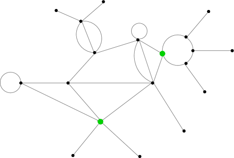
Figure 3: An example of foliation graph. Regular (a.k.a type I) vertices are represented by black dots, while exceptional (a.k.a. type II) vertices are represented by green blobs. All terminal vertices are regular vertices and correspond to center singularities. Notice that the graph can have multiple edges as well as loops.

Let ${\rm deg}\Delta_{s}$ denote the degree (valency) of $\Delta_{s}$ as a vertex of the foliation graph. A regular vertex $\Delta_{s}$ can be of two types:

• A center singularity $\Delta_{s}=\{p\}$ (with $p\in\Sigma_{0}({\boldsymbol{\omega}})$), when ${\rm deg}\Delta_{s}=1$. In this case, $\Delta_{s}$ is a terminal vertex of $\Gamma_{\boldsymbol{\omega}}$.

• A compact singular leaf when ${\rm deg}\Delta_{s}\geq 2$.

Every exceptional vertex is a union of minimal components, singular points and compactifiable non-compact leaves of $\mathcal{F}_{\boldsymbol{\omega}}$. For any vertex $\Delta_{s}$ of the foliation graph, we have Gelbukh7 :

$$|\Delta_{s}\cap\Sigma_{1}^{\mathrm{sp}}({\boldsymbol{\omega}})|\geq{\rm deg}\Delta_{s}+2m_{\Delta_{s}}-2~{}~{},$$

where $m_{\Delta_{s}}$ is the number of minimal components contained in $\Delta_{s}$. In particular, a regular vertex with ${\rm deg}\Delta_{s}>2$ is a compact singular leaf which contains at least one splitting strong saddle singularity. The number of edges $e(\Gamma_{\boldsymbol{\omega}})$ equals $N_{\mathrm{max}}({\boldsymbol{\omega}})$ while the number of vertices $v(\Gamma_{\boldsymbol{\omega}})$ equals $v({\boldsymbol{\omega}})$. Furthermore, it was shown in Gelbukh8 that the cycle rank $b_{1}(\Gamma_{\boldsymbol{\omega}})$ equals $c({\boldsymbol{\omega}})$. Thus:

$$e(\Gamma_{\boldsymbol{\omega}})=N_{\mathrm{max}}({\boldsymbol{\omega}})~{}~{},~{}~{}v(\Gamma_{\boldsymbol{\omega}})=v({\boldsymbol{\omega}})\leq|\mathrm{Sing}({\boldsymbol{\omega}})|~{}~{},~{}~{}b_{1}(\Gamma_{\boldsymbol{\omega}})=c({\boldsymbol{\omega}})~{}~{}.$$

The graph Euler identity $e(\Gamma_{\boldsymbol{\omega}})=v(\Gamma_{\boldsymbol{\omega}})+b_{1}(\Gamma_{\boldsymbol{\omega}})-1$ implies:

$$N_{\mathrm{max}}({\boldsymbol{\omega}})=c({\boldsymbol{\omega}})+v({\boldsymbol{\omega}})-1\leq c({\boldsymbol{\omega}})+|\mathrm{Sing}({\boldsymbol{\omega}})|-1~{}~{},$$

where we noticed that $v({\boldsymbol{\omega}})\leq|\mathrm{Sing}({\boldsymbol{\omega}})|$ since each $\Delta_{s}$ contains at least one singular point. An example of foliation graph is depicted in Figure 3.

Constraints on the foliation graph from the irrationality rank of ${\boldsymbol{\omega}}$.

When the chiral locus $\mathcal{W}$ is empty (i.e. when ${\boldsymbol{\omega}}$ is nowhere-vanishing) we have $\mathrm{Sing}({\boldsymbol{\omega}})=\emptyset$ and ${\bar{\mathcal{F}}}_{\boldsymbol{\omega}}=\mathcal{F}_{\boldsymbol{\omega}}$ is a regular foliation. Even though this doesn’t fit our assumption $\mathrm{Sing}{\boldsymbol{\omega}}\neq\emptyset$, one can define a (degenerate) foliation graph also in this situation (which was considered in g2 ). In this case, knowledge of the irrationality rank of $\mathfrak{f}$ determines the topology of the foliation $\mathcal{F}_{\boldsymbol{\omega}}$ for any ${\boldsymbol{\omega}}\in\mathfrak{f}$. Namely, one has only two possibilities (see Figure 4):

• $\rho(\mathfrak{f})=1$, i.e. $\mathfrak{f}$ is projectively rational. Then there exists exactly one maximal component (which coincides with $M$) and no minimal component. The foliation “graph” consists of one loop and has no vertices; $M$ is a fibration over $S^{1}$ as a consequence of Tischler’s theorem Tischler .

• $\rho(\mathfrak{f})>1$, i.e. $\mathfrak{f}$ is projectively irrational. There exists exactly one minimal component (which coincides with $M$) and no maximal component, i.e. $\mathcal{F}_{\boldsymbol{\omega}}$ is a minimal foliation. Then the foliation graph consists of a single exceptional vertex and every leaf of $\mathcal{F}_{\boldsymbol{\omega}}$ is dense in $M$. As explained in g2 , the noncommutative geometry of the leaf space is described by the $C^{\ast}$ algebra $C(M/\mathcal{F}_{\boldsymbol{\omega}})$ of the foliation, which is a non-commutative torus of dimensions $\rho({\boldsymbol{\omega}})$. Notice that this refined topological information is not reflected by the foliation graph.

​​​​​

​​​​​

(a) Foliation graph when $\mathcal{W}=\emptyset$ and $\rho({\boldsymbol{\omega}})=1$.

(b) Foliation graph when $\mathcal{W}=\emptyset$ and $\rho({\boldsymbol{\omega}})>1$.

Figure 4: Degenerate foliation graphs in the everywhere non-chiral case.

The situation is much more complicated when $\mathrm{Sing}({\boldsymbol{\omega}})$ is non-empty, in that knowledge of $\rho({\boldsymbol{\omega}})$ does not suffice to specify the topology of the foliation. In this case, knowledge of $\rho(\mathfrak{f})$ allows one to say only the following:

• When $\rho(\mathfrak{f})=1$, then the foliation $\mathcal{F}_{\boldsymbol{\omega}}$ is compactifiable for any ${\boldsymbol{\omega}}\in\mathfrak{f}$ FKL and the inequality (75) below requires $c({\boldsymbol{\omega}})\geq 1$. Hence the foliation graph $\Gamma_{\boldsymbol{\omega}}$ has only regular vertices and must have at least one cycle. Except for this, nothing else can be said about $\mathcal{F}_{\boldsymbol{\omega}}$ only by knowing that $\rho(\mathfrak{f})=1$. Indeed, it was shown in Gelbukh8 that any compactifiable Morse form foliation $\mathcal{F}_{{\boldsymbol{\omega}}^{\prime}}$ with $c({\boldsymbol{\omega}}^{\prime})\geq 1$ can be realized as the foliation defined by a Morse form ${\boldsymbol{\omega}}$ belonging to a projectively rational cohomology class. It was also shown in loc. cit. that such a foliation can in fact be realized by a Morse form of any irrationality rank lying between $1$ and $c({\boldsymbol{\omega}}^{\prime})$, inclusively.

• When $\rho(\mathfrak{f})>1$, then $\mathcal{F}_{\boldsymbol{\omega}}$ may be either compactifiable or non-compactifiable, hence the foliation graph may or may not have exceptional vertices; when $\mathcal{F}_{\boldsymbol{\omega}}$ is compactifiable, then $\Gamma_{\boldsymbol{\omega}}$ has no exceptional vertices and has a number of cycles at least equal to $\rho({\boldsymbol{\omega}})$. Criteria for compactifiability of $\mathcal{F}_{\boldsymbol{\omega}}$ can be found in FKL ; Gelbukh1 ; Gelbukh5 and are given below.

Theorem FKL ; Gelbukh1 ; Gelbukh5 .

The following statements are equivalent:

1. $\mathcal{F}_{\boldsymbol{\omega}}$ is compactifiable

2. The period morphism $\mathrm{per}_{\mathfrak{f}}:\pi_{1}(M)\rightarrow\mathbb{R}$ factorizes through a group morphism $\pi_{1}(M)\rightarrow K$, where $K$ is a free group

3. $H_{\boldsymbol{\omega}}^{\perp}\subset\ker{\boldsymbol{\omega}}$

4. ${\rm rk}\mathcal{H}_{\boldsymbol{\omega}}=\rho({\boldsymbol{\omega}})$.

The first criterion above is Proposition 2 in (FKL, , Sec. 8.2). Since $\mathcal{H}_{\boldsymbol{\omega}}\subset H_{\boldsymbol{\omega}}$, we have ${\rm rk}\mathcal{H}_{\boldsymbol{\omega}}\leq{\rm rk}H_{\boldsymbol{\omega}}=c({\boldsymbol{\omega}})$ and the theorem shows that compactifiability of $\mathcal{F}_{\boldsymbol{\omega}}$ requires:

$$\rho({\boldsymbol{\omega}})\leq c({\boldsymbol{\omega}})~{}~{}.$$ (75)

Remark.

By its construction, the foliation graph discards topological information about the restriction of the foliation to the minimal components of the Novikov decomposition, which are represented in the graph by exceptional vertices. As in the case $\mathrm{Sing}({\boldsymbol{\omega}})=\emptyset$, the $C^{\ast}$ algebra of the foliation should provide more refined information about the topology of ${\bar{\mathcal{F}}}_{\boldsymbol{\omega}}$ than the foliation graph. To our knowledge, this $C^{\ast}$ algebra has not been computed for foliations given by a Morse 1-form.

The oriented foliation graph.

For each maximal component $C_{j}^{\mathrm{max}}$, the diffeomorphism (74) can be chosen such that the sign of the integral $\int_{\gamma_{j}}{\boldsymbol{\omega}}$ is positive along any smooth curve $\gamma_{j}:(0,1)\rightarrow C^{\mathrm{max}}_{j}$ which projects to the interval $(0,1)$. Identifying the corresponding edge $e_{j}$ with this interval, this gives a canonical orientation $\vec{e}_{j}$ of $e_{j}$ which corresponds to “moving along $e_{j}$ in the direction of increasing value if $h_{j}$”, where $h_{j}$ is any locally-defined smooth function on an open subset of $C^{\mathrm{max}}_{j}$ whose exterior derivative equals ${\boldsymbol{\omega}}$. It follows that the foliation graph $\Gamma_{\boldsymbol{\omega}}$ admits a canonical orientation, which makes it into the oriented foliation graph $\vec{\Gamma}_{\boldsymbol{\omega}}$.

Weights on the oriented foliation graph.

Using the canonical orientation, the integrals:

$$w_{j}\stackrel{{\scriptstyle{\rm def.}}}{{=}}\int_{\gamma_{j}}{\boldsymbol{\omega}}$$ (76)

(whose value does not depend on the choice of $\gamma_{j}$ as above) provide canonical positive weights on $\vec{\Gamma}_{\boldsymbol{\omega}}$ FKL ; Honda . These weights can be used Gelbukh3 to describe the set of Morse 1-forms ${\boldsymbol{\omega}}$ which have the property that ${\bar{\mathcal{F}}}_{\boldsymbol{\omega}}=\bar{\mathcal{F}}$ for a fixed singular foliation $\bar{\mathcal{F}}$.

Expression for the weights in terms of $\mathbf{b}$ and $\mathbf{f}$.

In our application, the vector field $n={\hat{V}}^{\sharp}\in\Gamma(T\mathcal{U})$ is orthogonal to the leaves of $\mathcal{F}$ and satisfies:

$$n\lrcorner{\boldsymbol{\omega}}=4\kappa e^{3\Delta}||V||=n\lrcorner\mathbf{f}-\partial_{n}\mathbf{b}\geq 0~{}~{}$$ (77)

as a consequence of (47). Equality with zero in the right hand side occurs only at the points of $\mathcal{W}=\mathrm{Sing}({\boldsymbol{\omega}})$. It follows that the orientation of the edges of the foliation graph is in the direction of $n$ and that we can take $\gamma_{j}$ to be any integral curve $\ell_{j}$ of the vector field $n|_{C_{j}^{\mathrm{max}}}$. Relation (77) gives:

$$w_{j}=\mathbf{b}_{j}(\gamma_{j}(1))-\mathbf{b}_{j}(\gamma_{j}(0))+\int_{\gamma_{j}}\mathbf{f}~{}~{}.$$

When $\mathcal{F}_{\boldsymbol{\omega}}$ is compactifiable, this relation implies that the sum of weights along all edges of a cycle of the oriented foliation graph $\vec{\Gamma}_{\boldsymbol{\omega}}$ equals the period of $\mathfrak{f}$ along the corresponding homology 1-cycle $\alpha\in H_{1}(M)$ of $M$:

$$\sum_{\vec{e}_{j}~{}\mathrm{in~{}a~{}cycle~{}of~{}}\vec{\Gamma}_{\boldsymbol{\omega}}}w_{j}=\int_{\alpha}\mathfrak{f}~{}~{}.$$

4.8 The fundamental group of the leaf space

Even though the quotient topology of the leaf space $M/{\bar{\mathcal{F}}}_{\boldsymbol{\omega}}$ can be very poor, one can use the classifying space $\mathcal{G}$ of the holonomy pseudogroup of the regular foliation $\mathcal{F}_{\boldsymbol{\omega}}$ Hclass to define the fundamental group of the leaf space through Levitt3 :

$$\pi_{1}(M/\bar{\mathcal{F}}_{\boldsymbol{\omega}})\stackrel{{\scriptstyle{\rm def.}}}{{=}}\pi_{1}(B\mathcal{G})~{}~{}.$$

Notice that $B\mathcal{G}$ is an Eilenberg-MacLane space of type $K(\pi,1)$ Hclass , (i.e. all its homotopy groups vanish except for the fundamental group) since $\mathcal{F}_{\boldsymbol{\omega}}$ is defined by a closed one-form and hence the holonomy groups of its leaves are trivial. One finds Levitt3 :

$$\pi_{1}(M/\bar{\mathcal{F}}_{\boldsymbol{\omega}})=\pi_{1}(M)/\mathcal{L}_{\boldsymbol{\omega}}~{}~{},$$

where $\mathcal{L}_{\boldsymbol{\omega}}$ is the smallest normal subgroup of $\pi_{1}(M)$ which contains the fundamental group of each leaf of $\mathcal{F}_{\boldsymbol{\omega}}$. Notice that $M\setminus\mathrm{Sing}({\boldsymbol{\omega}})$ is connected (since $M$ is) and that the inclusion induces an isomorphism $\pi_{1}(M\setminus\mathrm{Sing}({\boldsymbol{\omega}}))\simeq\pi_{1}(M)$, since we assume $\dim M\geq 3$ and hence $\mathrm{Sing}{\boldsymbol{\omega}}$ has codimension at least 3 in $M$. In particular, the period map of ${\boldsymbol{\omega}}$ can be identified with that of ${\boldsymbol{\omega}}|_{M\setminus\mathrm{Sing}({\boldsymbol{\omega}})}$. Since ${\boldsymbol{\omega}}$ vanishes along the leaves of $\mathcal{F}_{\boldsymbol{\omega}}$, this map factors through the projection $\pi_{1}(M)\rightarrow\pi_{1}(M/\bar{\mathcal{F}}_{\boldsymbol{\omega}})$, inducing a map $\mathrm{per}_{0}({\boldsymbol{\omega}}):\pi_{1}(M/\bar{\mathcal{F}}_{\boldsymbol{\omega}})\rightarrow\mathbb{R}$.

A minimal component $C^{\mathrm{min}}_{a}$ is called weakly complete Levitt3 if any curve $\gamma\subset C^{\mathrm{min}}_{a}$ contained in $C^{\mathrm{min}}_{a}$ and for which $\int_{\gamma}{\boldsymbol{\omega}}$ vanishes has its two endpoints on the same leaf of $\mathcal{F}_{\boldsymbol{\omega}}$; various equivalent characterizations of weakly complete minimal components can be found in loc. cit. Let:

• $N^{\prime}_{\mathrm{min}}({\boldsymbol{\omega}})$ denote the number of minimal components which are not weakly complete

• $N^{\prime\prime}_{\mathrm{min}}({\boldsymbol{\omega}})$ denote the number of minimal components which are weakly complete

• $C^{\mathrm{min}}_{a_{1}},\ldots,C^{\mathrm{min}}_{a_{k}}$ (where $1\leq a_{1}<\ldots<a_{N^{\prime\prime}_{\mathrm{min}}({\boldsymbol{\omega}})}\leq N_{\mathrm{min}}({\boldsymbol{\omega}})$) denote those minimal components of the Novikov decomposition which are weakly complete

• ${\boldsymbol{\omega}}_{j}\stackrel{{\scriptstyle{\rm def.}}}{{=}}{\boldsymbol{\omega}}|_{C^{m}_{a_{j}}}$ denote the restriction of ${\boldsymbol{\omega}}$ to the weakly complete minimal component $C^{\mathrm{min}}_{a_{j}}$

• $\Pi_{j}({\boldsymbol{\omega}})\stackrel{{\scriptstyle{\rm def.}}}{{=}}\Pi({\boldsymbol{\omega}}_{j})$ denote the period group of ${\boldsymbol{\omega}}_{j}$. Then $\Pi_{j}({\boldsymbol{\omega}})$ is a free Abelian group of rank ${\rm rk}\Pi_{j}({\boldsymbol{\omega}})=\rho(\omega_{j})\geq 2$ Levitt3 .

With these notations, it was shown in Levitt3 that $\pi_{1}(M/\bar{\mathcal{F}}_{\boldsymbol{\omega}})$ is isomorphic with a free product of free Abelian groups:

$$\pi_{1}(M/\bar{\mathcal{F}}_{\boldsymbol{\omega}})\simeq F_{\boldsymbol{\omega}}\ast\Pi_{1}({\boldsymbol{\omega}})\ast\ldots\ast\Pi_{N^{\prime\prime}_{\mathrm{min}}({\boldsymbol{\omega}})}({\boldsymbol{\omega}})~{}~{},$$

where $\ast$ denotes the free product of groups. Furthermore Levitt3 ; Gelbukh2 , the free group $F_{\boldsymbol{\omega}}$ factors as:

$$F_{\boldsymbol{\omega}}\simeq\pi_{1}(\Gamma_{\boldsymbol{\omega}})\ast\mathbb{Z}^{\ast K({\boldsymbol{\omega}})}~{}~{},$$

where $\pi_{1}(\Gamma_{\boldsymbol{\omega}})\simeq\mathbb{Z}^{\ast c({\boldsymbol{\omega}})}$ is the fundamental group of the foliation graph and $K({\boldsymbol{\omega}})$ is a non-negative integer which satisfies $K({\boldsymbol{\omega}})\geq N^{\prime}_{\mathrm{min}}({\boldsymbol{\omega}})$ and $K({\boldsymbol{\omega}})+c({\boldsymbol{\omega}})+N^{\prime\prime}_{\mathrm{min}}({\boldsymbol{\omega}})\leq b^{\prime}_{1}(M)$. Here, $b^{\prime}_{1}(M)$ denotes the first noncommutative Betti number of $M$ Levitt1 , whose definition is recalled in Appendix E (which also summarizes some further information on the topology of $\bar{\mathcal{F}}$).

4.9 On the relation to compactifications of M-theory on 7-manifolds

One way in which one may attempt to think about our class of compactifications is via a two-step reduction of eleven-dimensional supergravity, as follows:

1. First, reduce eleven-dimensional supergravity along a leaf of the foliation down to a supergravity theory in four dimensions; this would of course be a gauged supergravity theory since the restrictions of $F$ and $f$ to a leaf are generally non-trivial.

2. Further reduce the resulting four-dimensional theory down to three dimensions, along the “one-dimensional space” orthogonal to the leaf.

This way of thinking, which corresponds to an attempt at generalizing the well-known, but much simpler case of “generalized Scherk-Schwarz compactifications with a twist” (see, for example, Vandoren ), turns out to be rather naive, for the following reasons:

• In the general case when $\mathcal{W}$ is nonempty and differs from $M$, there is no such thing as a “typical leaf” of the regular foliation $\mathcal{F}$ of $\mathcal{U}=M\setminus\mathcal{W}$, in the sense that the leaves of this foliation are not all diffeomorphic with each other. As explained above, what happens instead is that the leaves of the restriction of $\mathcal{F}$ to each of the maximal or minimal components of the Novikov decomposition of M are diffeomorphic with each other, which means that for each component of the Novikov decomposition one generally has a distinct diffeomorphism class of leaves. As such, it is unclear which of these seven-manifolds one is supposed to reduce on in step 1 above. Furthermore, the extended foliation $\bar{\mathcal{F}}$ also contains singular leaves, and it is not immediately clear (from a Physics perspective) how to correctly reduce eleven-dimensional supergravity, in the presence of fluxes, on such singular seven-manifolds. One should also note that the leaves of the restriction of $\mathcal{F}$ to a minimal component of the Novikov decomposition are non-compact, so the reduction along such leaves cannot be understood as a Kaluza-Klein reduction in the ordinary sense.

• In general, there is no nice “one-dimensional space” transverse to the leaves. As explained above, the best candidate for such a space is a non-commutative space whose “commutative parts” can be described by the foliation graph, but where some unknown non-commutative pieces have to be pasted in at the exceptional vertices. It is of course already unclear how to correctly reduce a four-dimensional supergravity theory on a graph, let alone on a non-commutative space.

As pointed out in (g2, , Subsection 4.4.), many of the issues mentioned above already appear in the much simpler case when $\xi$ is everywhere non-chiral. In that situation, the foliation graph is either a circle (and the Novikov decomposition is reduced to a single maximal component, all leaves being compact and mutually diffeomorphic, being the fibers of a fibration over the circle) or a non-commutative torus of dimension given by the projective irrationality rank of ${\boldsymbol{\omega}}$ (in which case the Novikov decomposition is reduced to a single minimal component, all leaves being non-compact, mutually diffeomorphic and dense in $M$). Only the first of these two cases has a chance at a meaningful interpretation as a “generalized Scherk-Schwarz compactification with a twist”, where the twist is provided by the Ehresmann connection discussed in (g2, , Appendix E), whose parallel transport generates the defining diffeomorphism $\phi_{a_{\mathfrak{f}}}$ which presents $M$ as a mapping torus in that case (see (g2, , Subsection 4.2)). A proper analysis of that case (which is the simplest of this class of compactifications) is already considerably more subtle than might seem at first sight, for the following reason. As shown in (g2, , Subsection 2.6), the restriction of $\xi$ to a leaf $L$ of $\mathcal{F}$ induces the spinor $\eta_{0}$ of equation (45) (see also (g2, , eq. (2.21))) which, as shown in loc. cit., is the normalized Majorana spinor (in the seven-dimensional sense) along the seven-manifold $L$ which induces its $G_{2}$ structure and which should be used to perform the compactification of eleven-dimensional supergravity on $L$ – a reduction which would constitute the first step outlined above. Notice, however, that what one needs in our case is not the standard $\mathcal{N}=1$ compactification of eleven-dimensional supergravity on a 7-manifold with $G_{2}$ structure which is usually considered in the literature following Minasian , since the latter is a compactification down to four-dimensional Minkowski space — while what would be needed in our case would be a compactification down to a space which is related to $\mathrm{AdS}_{3}\times S^{1}$. Also recall from (g2, , Subsection 2.6) that $\eta_{0}$ is a Majorana (a.k.a. real) spinor on $L$ (in the seven-dimensional sense) with respect to a real structure which is dependent of the precise leaf $L$ under consideration and not only of its diffeomorphism class. In particular, the $G_{2}$ structure depends on the leaf $L$ (it varies from leaf to leaf) in the complicated manner described by Theorems 1 and 2 of g2 and it is not invariant under the parallel transport of the Ehresmann connection mentioned above, so proper analysis of the second step of the reduction is considerably more involved than what one might expect based on analogy with previous work on Scherk-Schwarz-like constructions.

A conceptually better (and more uniform) way to think of the “relation to seven-dimensional compactifications” (beyond the results of g2 and of this paper, which can be viewed as already providing such a relation since they express very explicitly the geometry of $M$ in terms of the seven-dimensional geometry of the leaves of the foliation) is to consider the “partial decompactification limit” in which the leaf space is “large”. The correct way to formulate this mathematically employs the theory of adiabatic limits of foliations (see, for example, Kordyukov ), which, in its most general form, concerns their behavior when the leaf space (understood, in general, as a non-commutative space) is “large” in an appropriate spectral sense. This relates to extending the ordinary adiabatic argument (which lies behind a proper Kaluza-Klein formulation of the idea of “two-step reduction”) to the case of foliations. Though this subject is well-outside the scope of the present paper, we mention that such a way of formulating the problem leads to non-trivial mathematical questions given the fact that the adiabatic limit of foliations is poorly understood for the case of foliations which are not Riemannian, such as those which are of interest in our case (see Remark 3 after Theorem 2 of reference g2 ). The adiabatic limit for the general situation when one has to deal with a singular foliation $\bar{\mathcal{F}}$ does not seem to have been investigated in the Mathematics literature.

4.10 A non-commutative description of the leaf space ?

Recall from g2 that the leaf space of $\mathcal{F}$ admits a very explicit description as a non-commutative torus in the everywhere non-chiral case (the case $\mathcal{U}=M$, when the foliation graph is reduced either to a circle or to a single exceptional vertex). This leads to the speculation Levitt3 that the topological information which is lost when constructing the exceptional vertices of the foliation graph in the general case could be encoded by some sort of non-commutative geometry, as expected from the fact that such vertices are constructed by collapsing at least one minimal component of the Novikov decomposition to a single point; since the minimal components are foliated by dense leaves, the $C^{\ast}$-algebra of their leaf space must be non-commutative. Unfortunately, it is non-trivial to make this expectation precise, because one also has to take into account the effect of the singular leaves of $\bar{\mathcal{F}}$, so progress on this question would first require giving a proper definition/construction of the $C^{\ast}$-algebras of singular foliations in the sense of Haefliger, a task which, to our knowledge, has not yet been carried out in the mathematics literature. One may hope that some modification of the construction of Androulidakis1 ; Androulidakis2 (which applies to singular foliations in the sense of Stefan-Sussmann) would lead to a solution of this problem for the case of Haefliger structures, a case which is logically orthogonal to that considered in loc. cit.

5 Conclusions and further directions

We studied $\mathcal{N}=1$ compactifications of eleven-dimensional supergravity down to $\mathrm{AdS}_{3}$ in the case when the internal part $\xi$ of the supersymmetry generator is not required to be everywhere non-chiral, but under the assumption that $\xi$ is not chiral everywhere. We showed that, in such cases, the Einstein equations require that the locus $\mathcal{W}$ where $\xi$ becomes chiral must be a set with empty interior and therefore of measure zero. The regular foliation of g2 is replaced in such cases by a singular foliation ${\bar{\mathcal{F}}}$ (equivalently, by a Haefliger structure on $M$) which “integrates” a cosmooth singular distribution (generalized bundle) $\mathcal{D}$ on $M$. The singular leaves of $\bar{\mathcal{F}}$ are precisely those leaves which meet the chiral locus $\mathcal{W}$, thus acquiring singularities on that locus.

We discussed the topology of such singular foliations in the generic case when ${\boldsymbol{\omega}}$ is a Morse one-form, showing that it is governed by the foliation graph of MelnikovaThesis ; MelnikovaGraph ; FKL . On the non-chiral locus, we compared the foliation approach of g2 with the $\mathrm{Spin}(7)_{\pm}$ structure approach of Tsimpis , giving explicit formulas for translating between the two methods and showing that they agree. It would be interesting to study what supplementary constraints — if any — may be imposed on the topology of $\bar{\mathcal{F}}$ (and on its foliation graph) by the supersymmetry conditions; this would require, in particular, a generalization of the work of FKL ; Honda .

The singular foliation $\bar{\mathcal{F}}$ is defined by a closed one-form ${\boldsymbol{\omega}}$ whose zero set coincides with the chiral locus. Along the leaves of $\bar{\mathcal{F}}$ and outside the intersection of the latter with $\mathcal{W}$, the torsion classes are determined by the fluxes g2 . For the singular leaves in the Morse case, this leads to a more complicated version of the problems which were studied in Kcones1 ; Kcones2 for metrics with $G_{2}$ holonomy (the case of torsion-free $G_{2}$ structures).

The backgrounds discussed in this paper display a rich interplay between spin geometry, the theory of G-structures, the theory of foliations and the topology of closed one-forms Farber . This suggests numerous problems that could be approached using the methods and results of reference g2 and of this paper — not least of which concerns the generalization to the case of singular foliations of the non-commutative geometric description of the leaf space. In this regard, we note that a complete solution of this problem requires extending the construction of the $C^{\ast}$ algebra of regular foliations to the case of singular foliations in the sense of Haefliger — a generalization which would be different from (and, in fact, “orthogonal” to) that performed in Androulidakis1 ; Androulidakis2 for the case of singular foliations in the sense of Stefan-Sussmann. This problem is unsolved already for the case of singular foliations defined by a Morse one-form (the difficulty being in how to deal with the singular leaves). It would be interesting to study quantum corrections to this class of backgrounds, with a view towards clarifying their effect on the geometry of $\bar{\mathcal{F}}$. As mentioned in the introduction, the class of backgrounds discussed here appears to be connected with the proposals of Grana and Bonetti , connections which deserve to be explored in detail.

One of the reasons why the class of backgrounds studied in this paper may be of wider interest is because, as pointed out in Tsimpis , the structure group of $M$ does not globally reduce to a a proper subgroup of $\mathrm{SO}(8)$. This is the origin of the phenomena discussed in this paper, which illustrate the limitations of the theory of classical G-structures as well as of the theory of regular foliations. In its classical form Chern , the former does not provide a sufficiently wide conceptual framework for a fully general global description of all flux compactifications.

Appendix A Proof of the topological no-go theorem

Lemma.

If $\kappa=0$, then $F$ and $f$ must vanish and $\Delta$ must be constant on $M$. Furthermore, both $\xi^{+}$ and $\xi^{-}$ must be covariantly constant on $M$ (and hence $\xi$ is also covariantly constant) and $b$ must be constant on $M$.

Proof. The scalar part of the Einstein equations takes the form MartelliSparks :

$$e^{-9\Delta}\Box e^{9\Delta}+72\kappa^{2}=\frac{3}{2}||F||^{2}+3||f||^{2}~{}~{}.$$

Integrating this by parts on $M$ when $\kappa=0$, implies that $F$ and $f$ must vanish while $\Delta$ must be constant on $M$. In this case $Q=0$ and $\mathbb{D}=\nabla^{S}$ so the supersymmetry conditions (5) reduce to the condition that $\xi$ is covariantly constant on $M$. Then (6) implies that each of $\xi^{+}$ and $\xi^{-}$ are covariantly constant and hence $b$ is constant on $M$ while $V,~{}Y$ and $Z$ are covariantly constant since $\nabla^{S}$ is a Clifford connection in the sense of BGV . Notice that both $\xi^{+}$ and $\xi^{-}$ can still be non-vanishing so we can still have $|b|<1$, in which case $V$ is also non-vanishing and we still have a global reduction of structure group to $G_{2}$ on $M$. $\blacksquare$

Proof of the Theorem. The argument is based on the results of Tsimpis . Let us assume that $\mathrm{Int}\mathcal{W}$ is non-empty. Then at least one of the subsets $\mathcal{W}^{+}$ and $\mathcal{W}^{-}$ has non-empty interior and we can suppose, without loss of generality, that $\mathrm{Int}\mathcal{W}^{+}\neq 0$. Let $U$ be an open non-void subset of $\mathcal{W}^{+}$. By the definition of $\mathcal{W}^{+}$, we must have $\xi=\xi^{+}$ and thus $b=+1$ and $V=0$ at any point of $\mathcal{W}^{+}$ and hence of $U$. Since the one-form $L$ of Tsimpis (which we denote by $L_{+}$) is given in terms of $V$ by expression (37), it follows that $L_{+}$ vanishes at every point of $U$. The second of equations (3.16) of Tsimpis (notice that we can use the differential equations of Tsimpis on the subset $U$ of $\mathcal{W}^{+}$ since $U$ is open) shows that the following relation holds on $U$:

$$e^{-12\Delta}\ast\mathrm{d}\ast\Big{(}e^{12\Delta}\frac{L_{+}}{1+L_{+}^{2}}\Big{)}-4\kappa\frac{1-L_{+}^{2}}{1+L_{+}^{2}}=0~{}~{}$$

and since $L_{+}|_{U}=0$ this gives $\kappa=0$. The Lemma now implies that $b$ is constant on $M$ and since the set $\mathcal{W}^{+}$ where $b$ equals $+1$ is non-void by assumption, it follows that $b=+1$ on $M$ i.e. that we must have $\mathcal{W}^{+}=M$, which is Case 1 in the Theorem. Had we assumed that $\mathrm{Int}\mathcal{W}^{-}$ were non-empty, we would have concluded in the same way that $\mathcal{W}^{-}=M$, which is Case 2 in the theorem.

The argument above shows that either Case 1 or Case 2 of the Theorem hold or that both $\mathcal{W}^{+}$ and $\mathcal{W}^{-}$ must have empty interior. If at least one of them is a non-empty set, then we are in Case 4 of the Theorem. If both of them are empty sets, then $\mathcal{U}$ coincides with $M$ by the definition of $\mathcal{U},\mathcal{W}^{+}$ and $\mathcal{W}^{-}$ and we are in Case 3. In Case 4, the fact that $\mathcal{W}^{\pm}$ have empty interiors and the fact that they are both closed and disjoint implies immediately that they are both contained in the closure of $U$ and hence so is their union $\mathcal{W}$. Since $M$ equals $\mathcal{U}\cup\mathcal{W}$, this implies that the closure of $\mathcal{U}$ equals $M$ i.e. that $\mathcal{U}$ is dense in $M$. By the definition of $\mathcal{U}$ and $\mathcal{W}$ we have $\mathcal{W}=M\setminus\mathcal{U}$ and, since $M$ is the closure of $\mathcal{U}$, this means that $\mathcal{W}$ is the frontier of $\mathcal{U}$. $\blacksquare$

Appendix B The case $\kappa=0$

For completeness, we briefly discuss the case $\kappa=0$ (which corresponds to compactifications down to Minkowski space $\mathbb{R}^{1,2}$).

B.1 When $M$ is compact

In this case, the lemma of Appendix A implies that $F$ and $f$ vanish while $\xi$ (thus also $V$) are covariantly constant on $M$ and hence $b$ (and thus the norm of $V$) are constant on $M$; furthermore, $\Delta$ is constant on $M$. The operator $\mathbb{D}$ of (5) reduces to $\nabla^{S}$ while $Q$ reduces to zero. Since $\nabla^{S}$ is a Clifford connection on $S$ while $\nabla\nu=0$, it follows that $\nabla^{S}$ commutes with $\gamma(\nu)$. Therefore, the supersymmetry equation $\nabla^{S}\xi=0$ implies $\nabla^{S}\xi^{\pm}=0$. When $\xi$ is non-chiral, this shows that the space of solutions $\dim\mathrm{\cal K}(\nabla^{S},0)$ must be at least two-dimensional provided that it is non-trivial. In fact, existence of a non-trivial and non-chiral solution of the supersymmetry equations (5) is equivalent with existence of two non-trivial chiral solutions of opposite chirality. Due to this fact, the non-chiral case corresponds to $\mathcal{N}=2$ (rather than $\mathcal{N}=1$) supersymmetry of the effective 3-dimensional theory. Notice that this phenomenon is specific to the Minkowski case $\kappa=0$, since the operator $\mathbb{D}$ does not commute with $\gamma(\nu)$ when $\kappa$ is non-vanishing. We thus distinguish the cases:

1. $\xi$ has definite chirality at some point (and hence at every point) of $M$, which amounts to $|b|=1$. Then the metric $g$ of $M$ has holonomy contained either in $\mathrm{Spin}(7)_{+}$ (when $\xi=\xi_{+}$, i.e. $b=+1$ and $\mathcal{W}=\mathcal{W}^{+}=M$, $\mathcal{U}=\mathcal{W}^{-}=0$, which is Case 1 of the topological no-go theorem of Subsection 2.3) or in $\mathrm{Spin}(7)_{-}$ (when $\xi=\xi^{-}$, i.e. $b=-1$ and $\mathcal{W}=\mathcal{W}^{-}=M$, $\mathcal{U}=\mathcal{W}^{+}=0$, which is Case 2 of the topological no-go theorem), while $V$ vanishes identically on $M$. As a consequence, the distribution $\mathcal{D}=\ker V$ has corank zero and coincides with $TM$; the foliation $\mathcal{F}$ becomes a codimension zero foliation consisting of a single leaf equal to $M$. These cases correspond to the classical limit of the well-known compactifications of Becker1 . The holonomy equals $\mathrm{Spin}(7)_{\pm}$ iff. $M$ is simply-connected (which is allowed in this case). Notice that this class of Minkowski compactifications cannot be viewed as the $\kappa\rightarrow 0$ limit of the compactifications considered in g2 (which correspond to Case 3 of the topological no-go theorem) or in this paper (which correspond to Case 4 of the topological no-go theorem). In particular, one cannot take the limit $\kappa\rightarrow 0$ of the formulas given in Theorems 1, 2, 3 of g2 (which only apply to Case 3 or to the regular foliation $\mathcal{F}$ of the non-chiral set $\mathcal{U}$ of Case 4), since one encounters division by zero.

   Remark.

   One can also consider for example the case when $\mathrm{\cal K}(\nabla^{S},0)\subset\Gamma(M,S^{+})$ has dimension 2, which corresponds to the classical limit of the compactifications considered in BeckerCY . In this case, $M$ has holonomy contained in $\mathrm{SU}(4)\subset\mathrm{Spin}(7)_{+}$, i.e. it is a Calabi-Yau fourfold. One can turn on fluxes by considering the leading quantum correction to the Bianchi identity for $\mathbf{G}$ in such a way as to preserve $\mathcal{N}=2$ supersymmetry BeckerCY (in which case $F$ must be a primitive $(2,2)$ form) or $\mathcal{N}=1$ supersymmetry (in which case $F$ satisfies a weaker constraint, see (TsimpisSU4, , Subsection 3.1)).

2. $\xi$ is nowhere chiral on $M$, which amounts to $|b|<1$ and thus $||V||\neq 0$. Then $\mathcal{D}=\ker V$ is the (corank one) kernel distribution of a non-trivial covariantly constant one-form. The metric $g$ of $M$ has holonomy contained in $G_{2}$, the $G_{2}$ group at every point $p\in M$ being contained in the subgroup of $\mathrm{SO}(T_{p}M,g_{p})\simeq\mathrm{SO}(8)$ consisting of those proper rotations which preserve the one-form $V_{p}\in T_{p}^{\ast}M$ (rotations which form the group $\mathrm{SO}(\mathcal{D}_{p},g_{p}|_{\mathcal{D}_{p}})\simeq\mathrm{SO}(7)$). The holonomy group at $p$ coincides with the intersection of the $\mathrm{Spin}(7)_{+}$ and $\mathrm{Spin}(7)_{-}$ subgroups given by the stabilizers of $\xi^{\pm}_{p}$. The regular foliation $\mathcal{F}$ has codimension one, the restriction of the metric to each leaf having holonomy contained in $G_{2}$. As explained above, such compactifications lead to an effective action having $\mathcal{N}=2$ supersymmetry in 3 dimensions. They can be viewed as the limit $\kappa\rightarrow 0$ of Case 3 of the topological no-go theorem (a case which was studied in g2 ), the supersymmetry enhancement arising at the value $\kappa=0$. In fact, when $||V||\neq 0$, one can immediately take the limit $\kappa\rightarrow 0$ in the formulas of Theorems 1,2 and 3 of loc. cit., since $\kappa$ appears at most linearly in those expressions (and hence the limit is manifest). Using the fact that $b=0$ while $\Delta$ and $||V||$ are constant in the limit of interest here, one immediately checks, for example, that Theorem 1 of g2 reduces to a tautology (since $F=0$) while Theorem 2 gives $H=A=0$, which is equivalent with the fact that $V$ is covariantly constant ($\nabla V=0$) as well as $\vartheta=0$ (in the notations of loc. cit.), which is equivalent with $D_{n}\varphi=D_{n}\psi=0$ (which is a consequence of the fact that $\mathcal{D}$ is the kernel distribution of a covariantly constant one-form) and $\boldsymbol{\tau}_{0}=\boldsymbol{\tau}_{1}=\boldsymbol{\tau}_{2}=\boldsymbol{\tau}_{3}=0$, which shows that the $G_{2}$ structure has trivial torsion classes, thus corresponding, as expected, to a metric whose restriction to the leaves of $\mathcal{F}$ has $G_{2}$ holonomy. Since $H=A=0$, it follows by Reinhart’s criterion that $\mathcal{F}$ is a Riemannian foliation (the metric $g$ is bundle-like for $\mathcal{F}$). Notice that such $\mathcal{N}=2$ Minkowski compactifications are different from the classical limit of the Calabi-Yau fourfold compactifications considered in BeckerCY , which instead correspond to the case when the two-dimensional space of solutions $\mathrm{\cal K}(\nabla^{S},0)$ consists of chiral spinors of the same chirality and hence arise as a particular case of 1. above. In the case discussed here $\mathrm{\cal K}(\nabla^{S},0)\subset\Gamma(M,S)$ is spanned by two chiral spinors of opposite chirality. As in BeckerCY , one could turn on fluxes in such Minkowski compactifications (while preserving $\mathcal{N}=2$ supersymmetry) by considering the quantum correction to the Bianchi identity of $\mathbf{G}$ which is induced by 5-brane anomaly cancellation, leading to a class of “first order corrected compactifications” which, in our opinion, deserve further study.

For reader’s convenience, we reproduce below some results of (g2, , Theorem 3) which are relevant for this discussion, where we use arrows to indicate the limit $\kappa=0$ with constant $\Delta$ and constant $b$ (as required by the lemma of Appendix A). Solving the supersymmetry conditions, i.e. finding at least one non-trivial solution $\xi$ for (5) which is everywhere non-chiral (and which can be taken to be everywhere of norm one) was shown in g2 to give the following constraints:

• On the fluxes $f\in\Omega^{1}(M)$ and $F\in\Omega^{4}(M)$:

  $$f = 4\kappa V+e^{-3\Delta}\mathrm{d}(e^{3\Delta}b)\rightarrow 0,$$

  $$F_{\perp} = \alpha_{1}\wedge\varphi-\hat{h}_{ij}e^{i}\wedge\iota_{e^{j}}\psi~{}~{},$$

  $$F_{\top} = -\iota_{\alpha_{2}}\psi+\chi_{ij}e^{i}\wedge\iota_{e^{j}}\varphi~{}~{},$$

  with:

  $$\alpha_{1}=\frac{1}{2||V||}(\mathrm{d}b)_{\perp}\rightarrow 0~{}~{} ~{}~{}\alpha_{2}=-\frac{b}{2||V||}(\mathrm{d}b)_{\perp}+\frac{3||V||}{2}(\mathrm{d}\Delta)_{\perp}\rightarrow 0~{}~{},$$ , (78)

  $$\mathrm{tr}_{g}(\hat{\chi})=\kappa-\frac{1}{2||V||}(\mathrm{d}b)_{\top}\rightarrow 0~{}~{} ~{}~{}\mathrm{tr}_{g}(\hat{h})=2\kappa b-\frac{3||V||}{2}(\mathrm{d}\Delta)_{\top}+\frac{b}{2||V||}(\mathrm{d}b)_{\top}\rightarrow 0~{}~{},~{}~{}$$ ,

  where:

  $$\hat{h}_{ij}=h^{(0)}_{ij}+\frac{1}{7}\mathrm{tr}_{g}(\hat{h})g_{ij}~{}~{}~{},~{}~{}~{}\chi_{ij}=\chi^{(0)}_{ij}+\frac{1}{7}\mathrm{tr}_{g}(\chi)g_{ij}~{}~{},~{}~{}~{}\mathrm{tr}_{g}(\chi)=-\frac{4}{3}\mathrm{tr}_{g}(\hat{\chi})~{}~{}.$$

  In the above limit, the fluxes vanish by the no-go theorem and one finds $\chi={\hat{h}}=0$.

• On the quantities $H$, $\mathrm{tr}A$ and $\vartheta$ of the foliation $\mathcal{F}$:

  $$H_{\sharp}=3(\mathrm{d}\Delta)_{\perp}-\frac{b}{||V||^{2}}(\mathrm{d}b)_{\perp}\rightarrow 0~{},$$

  $$\mathrm{tr}A=-\frac{8\kappa b}{||V||}+12(\mathrm{d}\Delta)_{\top}-\frac{b(\mathrm{d}b)_{\top}}{||V||^{2}}\rightarrow 0~{},$$

  $$\vartheta=\frac{b}{2}(\mathrm{d}\Delta)_{\perp}-\frac{1+b^{2}}{6||V||^{2}}(\mathrm{d}b)_{\perp}\rightarrow 0~{}~{},$$ (79)

• On the torsion classes (notice that $\boldsymbol{\tau}_{3}$ is not constrained) of the leafwise $G_{2}$ structure:

  $$\boldsymbol{\tau}_{0}=\frac{4}{7||V||}\Big{[}2\kappa(3+b^{2})-\frac{3b}{2}||V||(\mathrm{d}\Delta)_{\top}+\frac{1+b^{2}}{2||V||}(\mathrm{d}b)_{\top}\Big{]}\rightarrow 0~{},$$

  $$\boldsymbol{\tau}_{1}=-\frac{3}{2}(\mathrm{d}\Delta)_{\perp}\rightarrow 0~{}~{},~{}~{}~{}\boldsymbol{\tau}_{2}=0~{},~{}$$

  $$\boldsymbol{\tau}_{3}=\frac{1}{||V||}(\chi^{(0)}_{ij}-h^{(0)}_{ij})e^{i}\wedge\iota_{e^{j}}\varphi\rightarrow 0~{}.$$ (80)

B.2 When $M$ is non-compact

Even though our interest is specifically in the case when $M$ is compact, it may be instructive to consider for the moment also the non-compact case (this is the only place in this paper where we shall do so). Let us assume that $M$ is non-compact but connected and paracompact. In this case, the lemma of Appendix A fails to hold (and hence non-vanishing fluxes are allowed) but the first part of the proof of the topological no-go theorem (which is independent of the lemma) still applies, showing the the condition $\kappa\neq 0$ still requires that the closed sets $\mathcal{W}^{+}$ and $\mathcal{W}^{-}$ have empty interior. When $\kappa=0$, however, any of these sets may acquire interior points. In that case, one has a background given by a warped product of $\mathbb{R}^{1,2}$ with the non-compact Riemannian manifold $(M,g)$ and we have $\mathbf{f}=\mathrm{d}\mathbf{b}$ on $M$. The geometry can be described as follows upon using the chirality decomposition $M=\mathcal{U}\sqcup\mathcal{W}^{+}\sqcup\mathcal{W}^{-}$ (we must of course assume that the warp factor $\Delta$ is smooth on $M$ also in the Minkowski limit, in order to have a meaningful physical interpretation in supergravity):

• The open submanifold $\mathcal{U}$ of $M$ can support non-vanishing fluxes $F|_{\mathcal{U}}$ and $f|_{\mathcal{U}}$ and carries a regular codimension one foliation $\mathcal{F}$ (the foliation which integrates the kernel distribution of the one-form $V|_{\mathcal{U}}$) endowed with a longitudinal $G_{2}$ structure, whose geometry is determined by the case $\kappa=0$ of Theorems 2, 3 of reference g2 . This is the non-compact version of the solutions discussed at point 2 of the previous subsection. Notice that both $b$ and $\Delta$ may be non-constant in the non-compact case and hence the limit $\kappa\rightarrow 0$ (which is again trivial to take) is slightly different from that given in the previous subsection.

• Up to a conformal transformation, the restriction $g|_{\mathrm{Int}\mathcal{W}^{+}}$ has holonomy contained in $\mathrm{Spin}(7)_{+}$, the type of the solution along $\mathrm{Int}\mathcal{W}^{+}$ being, locally, the classical limit (the limit when the effect of the tadpole term induced by 5-brane anomaly cancellation in M-theory is neglected) of the non-compact version of the solution considered in Becker1 ; in particular, the restriction $F|_{\mathcal{W}^{+}}$ is self-dual while the restriction of $f$ to $\mathcal{W}^{+}$ is completely determined by the warp factor, as in loc. cit. These conclusions follow either from the computations of Becker1 (computations which are local in nature and hence apply on $\mathrm{Int}\mathcal{W}^{+}$) or more directly by setting $\kappa=0,b=+1,V=L=0$ in the results of Appendix C, which gives $F|_{\mathcal{W}^{+}}=F^{[27]}|_{\mathcal{W}^{+}}$ and $\theta_{+}=-6\mathrm{d}\Delta$, $T_{+}=\ast(\Phi^{+}\wedge\mathrm{d}\Delta)$ on this locus (see the last remark in that appendix).

• The restriction of $F|_{\mathcal{W}^{-}}$ is anti-selfdual while $g|_{\mathrm{Int}\mathcal{W}^{-}}$ is conformally of holonomy contained in $\mathrm{Spin}(7)_{-}$, the type of the solution along $\mathrm{Int}\mathcal{W}^{-}$ being, locally, the classical limit of the non-compact version of the solutions considered in Becker1 , up to a change of orientation of $\mathrm{Int}\mathcal{W}^{-}$.

Notice that the one-form $V$ vanishes along $\mathcal{W}^{+}$ and $\mathcal{W}^{-}$ but that it does not vanish anywhere on $\mathcal{U}$. In general, the closures $\mathcal{W}^{\pm}$ of the open submanifolds $\mathrm{Int}\mathcal{W}^{\pm}$ need not themselves be manifolds, since the frontiers $\mathrm{Fr}(\mathcal{W}^{\pm})=\mathrm{fr}(\mathcal{W}^{\pm})$ could be quite “wild”, i.e. quite far from being immersed submanifolds of $M$. Globally, the geometry of $M$ can be described by saying that $M$ admits a metric-compatible “cosmooth generalized G-structure of type $(G_{2},\mathrm{Spin}(7)_{+},\mathrm{Spin}(7)_{-})$, supported on $(\mathcal{U},\mathrm{Int}\mathcal{W}^{+},\mathrm{Int}\mathcal{W}^{-})$”, where the of the $\mathrm{Spin}(7)_{\pm}$ components are conformally parallel. As in Subsection 2.8, one can pack this information into a Haefliger structure, which amounts, geometrically, to adding “singular leaves” to the foliation $\mathcal{F}$, thus completing it to a singular foliation $\bar{\mathcal{F}}$. Namely, $\bar{\mathcal{F}}$ will contain supplementary leaves of codimension one which meet the frontier $\mathrm{Fr}(\mathcal{W})=\mathrm{fr}(\mathcal{W})$ (being singular there) as well as supplementary leaves of codimension zero (dimension eight) which are given by the connected components of the open sets $\mathrm{Int}\mathcal{W}^{\pm}$. The latter are open submanifolds of $M$ whose induced metric has $\mathrm{Spin}(7)_{\pm}$ holonomy. When the form ${\boldsymbol{\omega}}$ is Morse, the sets $\mathcal{W}^{+}$ and $\mathcal{W}^{-}$ are finite (and hence have empty interior) and the second kind of supplementary leaves do not appear; in this case, one has a codimension one Morse form foliation of the non-compact manifold $M$, which can again be described using a foliation graph. The geometric description given above could be used, in principle, to attempt a mathematical classification of all non-compact backgrounds given by warped products $\mathrm{AdS}_{3}\times_{\Delta}M$, but such a study lies well outside the scope of the present paper.

Remark.

Note that $F$ and $f$ need not be “small” on the locus $\mathcal{U}$ in this class of non-compact Minkowski reductions. The small flux approximation (with $M$ non-compact) along the locus $\mathrm{Int}\mathcal{W}^{+}$ was studied in Tsimpis .

Appendix C Comparison with the results of Tsimpis

Recall that the positive chirality component $\xi^{+}$ of $\xi$ is non-vanishing along the locus $\mathcal{U}^{+}$ and hence defines a $\mathrm{Spin}(7)_{+}$ structure on the open submanifold $\mathcal{U}$ of $M$. The locus $\mathcal{U}^{+}$ was studied in Tsimpis using this $\mathrm{Spin}(7)_{+}$ structure. In this appendix, we show that the results of Tsimpis agree with those of g2 along the non-chiral locus $\mathcal{U}$ when taking into account the relation between $L$ and $V$ given in Subsection 2.6 and the relation between the $G_{2}$ and $\mathrm{Spin}(7)_{+}$ parameterizations of the fluxes given in Subsection 3.2. Note that reference Tsimpis uses the notation $\Phi\stackrel{{\scriptstyle{\rm def.}}}{{=}}\Phi^{+}$ and $L\stackrel{{\scriptstyle{\rm def.}}}{{=}}L^{+}$. Accordingly, in this appendix we work only with the $\mathrm{Spin}(7)_{+}$ structure and we drop the “+” superscripts and subscripts indicating this structure. Only the major steps of some computations (many of which were performed using code based on the package Ricci Ricci for Mathematica^®) are given below.

Equations for $L$ ($V$).

Using the relation $L=\frac{1}{1+b}V$, equations (Tsimpis, , (3.16)) take the following form when written in an arbitrary local frame of $\mathcal{U}$:

$$\mathrm{d}\Big{(}e^{3\Delta}V\Big{)}=0~{}~{},~{}~{}e^{-12\Delta}\ast\mathrm{d}\ast(e^{12\Delta}V)-8\kappa b=0~{}~{}.$$ (81)

These coincide with the equations discussed in the Remarks after Theorem 3 of g2 .

Equations for fluxes in terms of $L$ ($V$).

The first two and last of relations (3.2) take the following coefficient form in the $\mathrm{Spin}(7)_{+}$ case, being equivalent with equations (Tsimpis, , (C.2)):

$$F^{[\bf{1}]}_{a_{1}a_{2}a_{3}a_{4}}=\frac{1}{42}\Phi_{a_{1}a_{2}a_{3}a_{4}}\mathcal{F}^{[\bf{1}]}~{}~{},$$

$$F^{[\bf{7}]}_{a_{1}a_{2}a_{3}a_{4}}=\frac{1}{24}\Phi_{[a_{1}a_{2}a_{3}}{}^{a}\mathcal{F}^{[\bf{7}]}_{a_{4}]a}~{}~{},$$ (82)

$$F^{[\bf{35}]}_{a_{1}a_{2}a_{3}a_{4}}=\frac{1}{6}\Phi_{[a_{1}a_{2}a_{3}}{}^{a}\mathcal{F}^{[\bf{35}]}_{a_{4}]a}~{}~{}.$$

Furthermore, the $\mathrm{Spin}(7)_{+}$ case of relation (55) has the following coefficient form, which is equivalent with (Tsimpis, , (C.1)):

$$F_{a_{1}a_{2}a_{3}a_{4}}{\Phi^{a_{1}a_{2}a_{3}}}_{a_{5}}=g_{a_{4}a_{5}}\mathcal{F}^{[{\bf 1}]}+\mathcal{F}^{[{\bf 7}]}_{a_{4}a_{5}}+\mathcal{F}^{[{\bf 35}]}_{a_{4}a_{5}}~{}~{}.$$ (83)

Reference Tsimpis uses the notations:

$$(P^{\bf{7}})_{rs}^{pq}\stackrel{{\scriptstyle{\rm def.}}}{{=}}\frac{1}{4}\left(\delta_{[r}^{p}\delta^{q}_{s]}-\frac{1}{2}\Phi_{rs}{}^{pq}\right)~{}~{},$$ (84)

$$(L\otimes\mathcal{F}^{[\bf{7}]})_{a_{1}a_{2}a_{3}}^{\bf{48}}=6\left(L_{[a_{1}}\mathcal{F}^{[\bf{7}]}_{a_{2}a_{3}]}+\frac{1}{7}\Phi_{a_{2}a_{2}a_{3}}{}^{b}L^{a}\mathcal{F}^{[\bf{7}]}_{ab}\right)\Longleftrightarrow(L\otimes\mathcal{F}^{[\bf{7}]})^{\bf{48}}=2L\wedge\mathcal{F}^{[\bf{7}]}-\frac{1}{7}\iota_{\iota_{L}\mathcal{F}^{[\bf{7}]}}\Phi~{},$$

$$(L\otimes F^{[\bf{27}]})_{a_{1}a_{2}a_{3}}^{\bf{48}}\stackrel{{\scriptstyle{\rm def.}}}{{=}}L^{a}F^{[\bf{27}]}_{aa_{1}a_{2}a_{3}}~{}~{}~{}\mathrm{i.e.}~{}~{}~{}L\otimes F^{[\bf{27}]}\stackrel{{\scriptstyle{\rm def.}}}{{=}}\iota_{L}F^{[\bf{27}]}~{}~{}.$$

Using the relation $L=\frac{1}{1+b}V$ and the identity $||V||^{2}=1-b^{2}$, one computes, for example:

$$||L||^{2}\!\!=\frac{1-b}{1+b}~{}~{},~{}~{}1+||L||^{2}\!\!=\frac{2}{1+b}~{}~{},~{}~{}1-||L||^{2}\!\!=\frac{2b}{1+b}~{}~{},~{}~{}\frac{1-||L||^{2}}{1+||L||^{2}}\!\!=b~{}~{},~{}~{}\frac{L}{1+||L||^{2}}\!\!=\frac{1}{2}V~{}~{}.$$

Due to such identities, equations (Tsimpis, , (3.17)) take the form:

$$\begin{split}&f=e^{-3\Delta}\mathrm{d}(e^{3\Delta}b)+4\kappa V~{}~{},\\ &\frac{1}{12}\mathcal{F}^{[\bf{1}]}=\frac{||V||}{2(1+b)}e^{-3\Delta}[\mathrm{d}(e^{3\Delta}(1+b))]_{\top}-\kappa(1+2b)~{}~{},\\ &\frac{1}{96}\mathcal{F}^{[\bf{7}]}_{pq}=-\frac{1}{2(1+b)}e^{-3\Delta}(P^{\bf{7}})^{rs}_{pq}V_{r}\partial_{s}(e^{3\Delta}(1+b))~{}~{},\\ &\frac{1}{24}\mathcal{F}^{[\bf{35}]}_{pq}=-\frac{||V||}{1+b}\nabla_{(p}{\hat{V}}_{q)}+\frac{1+b^{2}}{2(1+b)||V||}{\hat{V}}_{(p}\nabla_{q)}b+\frac{3(1-b)||V||}{2(1+b)}{\hat{V}}_{(p}\nabla_{q)}\Delta+\mathbb{T}_{pq}-\\ &-\frac{1}{14(1+b)}\left[\frac{3(1-b)||V||}{1+b}(\mathrm{d}b)_{\top}+9(1-b)||V||(\mathrm{d}\Delta)_{\top}+8(1-b)(1+2b)\kappa\right]{\hat{V}}_{p}{\hat{V}}_{q}-\\ &-\frac{1}{14(1+b)}\left[\frac{(1-b)||V||}{2(1+b)}(\mathrm{d}b)_{\top}+\frac{3}{2}(15-2b)||V||(\mathrm{d}\Delta)_{\top}-(1+15b-2b^{2})\kappa\right]g_{pq}~{}~{},\end{split}~{}~{}$$ (85)

where the quantity $\mathbb{T}_{ab}$ (which appears in the last equation of (Tsimpis, , (3.17))) can be expressed as:

$$\mathbb{T}_{ab}\stackrel{{\scriptstyle{\rm def.}}}{{=}}-\frac{1}{4}\Phi_{(a}{}^{cde}(L\otimes F^{[\bf{27}]})^{\bf{48}}_{b)cd}L_{e}=\frac{1}{4}\Phi_{(a}{}^{cde}L^{f}F^{[{\bf 27}]}_{b)fcd}L_{e}=\frac{1-b}{2(1+b)}(\iota_{e^{(a}}\Phi)\bigtriangleup_{3}[(\iota_{e^{b)}}F^{[{\bf 27}]})_{\parallel}]~{}~{}.$$ (86)

In an orthonormal local frame with $e_{1}=n$, we have:

$$\mathbb{T}_{11}=\mathbb{T}_{1j}=\mathbb{T}_{j1}=0~{}~{},~{}~{}\mathbb{T}_{ij}=\frac{1-b}{2(1+b)}(\iota_{e^{(i}}\varphi)\bigtriangleup_{2}^{\perp}(\iota_{e^{j)}}F_{\top}^{[{\bf 27}]})=-\frac{1-b}{24(1+b)}\mathcal{F}^{[{\bf 27}]}_{ij}~{}~{}.$$

The first equation in (85) coincides with a relation given in Theorem 3 of g2 . The second equation in (85) can be written as:

$$\mathcal{F}^{[{\bf 1}]}=12\left[\frac{3||V||}{2}(\mathrm{d}\Delta)_{\top}+\frac{||V||}{2(1+b)}(\mathrm{d}b)_{\top}-\kappa(1+2b)\right]~{}~{},\\$$ (87)

while the third relation in (85) separates as follows into parts parallel and perpendicular to $n$:

$$\mathcal{F}_{\top}^{[{\bf 7}]}=-6||V||\left[3(\mathrm{d}\Delta)_{\perp}+\frac{(\mathrm{d}b)_{\perp}}{(1+b)}\right]~{}~{},$$

$$\mathcal{F}_{\perp}^{[{\bf 7}]}=6||V||\left[3\iota_{(\mathrm{d}\Delta)_{\perp}}\varphi+\frac{1}{1+b}\iota_{(\mathrm{d}b)_{\perp}}\varphi\right]~{}~{}.$$ (88)

In an orthonormal frame as above, we find that the last equation in (85) amounts to:

$$\mathcal{F}_{11}^{[\bf{35}]}=12\left[-\frac{3}{2}||V||(\mathrm{d}\Delta)_{\top}-\kappa(1-2b)+\frac{1+b}{2||V||}(\mathrm{d}b)_{\top}\right]~{}~{},$$

$$\mathcal{F}_{1i}^{[\bf{35}]}e^{i}=12\left[\frac{1+b}{2||V||}(\mathrm{d}b)_{\perp}-\frac{3}{2}||V||(\mathrm{d}\Delta)_{\perp}\right]~{}~{},$$ (89)

$$\frac{1}{2}\mathcal{F}_{ij}^{[\bf{35}]}e^{i}\odot e^{j}=\frac{12}{7}\left[\frac{3}{2}||V||(\mathrm{d}\Delta)_{\top}-\frac{1+b}{2||V||}(\mathrm{d}b)_{\top}+\kappa(1-2b)\right]g-12(h^{(0)}-\chi^{(0)})~{}~{}.$$

Substituting the expressions for $\alpha_{1},\alpha_{2}$ and ${\hat{h}},{\hat{\chi}}$ given in Theorem 3 of g2 , it is now easy to check that relations (87)-(C) are equivalent with:

$$\mathcal{F}^{[{\bf 1}]}=-12\mathrm{tr}({\hat{h}}+{\hat{\chi}})~{}~{},$$

$$\mathcal{F}_{\top}^{[{\bf 7}]}=-12(\alpha_{1}+\alpha_{2})~{}~{},$$

$$\mathcal{F}_{\perp}^{[{\bf 7}]}=~{}12\iota_{(\alpha_{1}+\alpha_{2})}\varphi~{}~{},$$

$$\mathcal{F}_{11}^{[\bf{35}]}=12\mathrm{tr}({\hat{h}}-{\hat{\chi}})~{}~{},$$ (90)

$$\mathcal{F}_{1i}^{[\bf{35}]}e^{i}=12(\alpha_{1}-\alpha_{2})~{}~{},$$

$$\frac{1}{2}\mathcal{F}_{ij}^{[\bf{35}]}e^{i}\odot e^{j}=-12({\hat{h}}-{\hat{\chi}})~{}~{},$$

which in turn are equivalent with (60) when $\mathcal{F}^{[{\bf k}]}$ are expressed in the $\mathrm{Spin}(7)_{+}$ parameterization using (56) and (57).

Remark.

To arrive at equations (C), one uses the relations:

$${\hat{V}}_{(1;1)}=0~{}~{},~{}~{}{\hat{V}}_{(1;j)}=\frac{1}{2}H_{j}~{}~{},~{}~{}{\hat{V}}_{(i;j)}=-A_{ij}~{}~{},$$ (91)

which can be derived by using the local expressions given in Appendix C of g2 . Notice that the tensor $\frac{1}{2}V_{(a,b)}e^{a}\odot e^{b}=\frac{1}{2}V_{a;b}e^{a}\odot e^{b}={\hat{V}}_{(a;b)}e^{a}\otimes e^{b}$ is the Hessian $\mathrm{Hess}({\hat{V}})$ of ${\hat{V}}$, where we remind the reader that we use conventions (1), which were also used in g2 .

Equations for the $\mathrm{Spin}(7)_{+}$ structure in terms of $V$ and of the fluxes.

Reference Tsimpis uses a one-form $\omega^{1}\in\Omega^{1}(M)$ and a three-form $\omega^{2}\in\Omega^{3}(M)$ which are given by (Tsimpis, , eq. (3.18)):

$$\begin{split}\!\!\!&\omega^{1}_{m}\!\!=\!\!\frac{\kappa}{2}L_{m}+\!\!\frac{3}{4}\partial_{m}\Delta+\!\!\frac{1}{168}(L_{m}\mathcal{F}^{[\bf{1}]}-\!\!L^{i}\mathcal{F}_{im}^{[\bf{7}]})~{}~{}\Leftrightarrow~{}\omega^{1}\!\!=\!\!\frac{\kappa}{2}L+\!\!\frac{3}{4}\mathrm{d}\Delta+\!\!\frac{1}{168}(\mathcal{F}^{[\bf{1}]}L-\!\!\iota_{L}\mathcal{F}^{[\bf{7}]})~{}~{},\\ \!\!\!&\omega^{2}_{mpq}\!\!=\!\!\frac{1}{192}(L\otimes\mathcal{F}^{[\bf{7}]})^{\bf{48}}_{mpq}+\!\!\frac{1}{4}(L\otimes F^{[\bf{27}]})^{\bf{48}}_{mpq}~{}\Leftrightarrow~{}\omega^{2}\!\!=\!\!\frac{1}{192}(2L\wedge\mathcal{F}^{[\bf{7}]}-\!\!\frac{6}{7}\iota_{\iota_{L}\mathcal{F}^{[\bf{7}]}}\Phi)+\!\!\frac{1}{4}\iota_{L}F^{[\bf{27}]}~{}.\end{split}$$ (92)

These forms satisfy the equation (cf. (Tsimpis, , eq. (3.15))):

$$\partial_{[m}\Phi_{pqrs]}=-8\Phi_{[mpqr}\omega^{1}_{s]}-\frac{4}{15}\varepsilon_{mpqrs}{}^{ijk}\omega^{2}_{ijk}~{}~{}\Longleftrightarrow~{}~{}\mathrm{d}\Phi=-8\Phi\wedge\omega^{1}+8\ast\omega^{2}~{}~{},$$ (93)

where to arrive at the coordinate-free relation we used the expression:

$$(\ast\omega^{2})_{mpqrs}=-\frac{1}{5!}\epsilon_{mpqrsabc}(\omega^{2})^{abc}~{}~{}.$$

Defining $\theta^{\prime}\in\Omega^{1}(M)$ and $T^{\prime}\in\Omega^{3}(M)$ through:

$$\omega^{1}\stackrel{{\scriptstyle{\rm def.}}}{{=}}-\frac{7}{48}\theta^{\prime}~{}~{},~{}~{}\omega^{2}\stackrel{{\scriptstyle{\rm def.}}}{{=}}-\frac{1}{8}T^{\prime}~{}~{},$$ (94)

equations (93) take the form:

$$\mathrm{d}\Phi=\frac{7}{6}\theta^{\prime}\wedge\Phi-\ast T^{\prime}~{}~{}.$$ (95)

Relation (64) tells us that the Lee-form $\theta$ and the characteristic torsion form $T$ of the $\mathrm{Spin}(7)_{+}$ structure form the particular solution of this inhomogeneous equation which also satisfies condition (63). It follows that $(\theta^{\prime},T^{\prime})$ must differ from $(\theta,T)$ through a solution $(\theta^{0},T^{0})$ of the homogeneous equation associated with (95), i.e. we must have:

$$\theta^{\prime}=\theta+\theta^{0}~{}~{},~{}~{}T^{\prime}=T+T^{0}~{}~{}\mathrm{with}~{}~{}T^{0}=-\frac{7}{6}\iota_{\theta^{0}}\Phi~{}~{},$$ (96)

where $\theta^{0}\in\Omega^{1}(M)$. Using (41), we find:

$$T^{0}_{\perp}=-\frac{7}{6}(\theta_{\top}^{0}\varphi+\iota_{\theta^{0}_{\perp}}\psi)~{}~{},~{}~{}T^{0}_{\top}=\frac{7}{6}\iota_{\theta^{0}_{\perp}}\varphi~{}~{}$$ (97)

and hence:

$$\boxed{\begin{split}&\omega^{1}_{\top}=-\frac{7}{48}(\theta_{\top}+\theta^{0}_{\top})~{}~{},~{}~{}\omega^{2}_{\top}=-\frac{1}{8}\left(T_{\perp}+\frac{7}{6}\iota_{\theta^{0}_{\perp}}\varphi\right)~{}~{}\\ &\omega^{1}_{\perp}=-\frac{7}{48}(\theta_{\perp}+\theta^{0}_{\perp})~{}~{},~{}~{}\omega^{2}_{\perp}=-\frac{1}{8}\left[T_{\top}-\frac{7}{6}(\iota_{\theta^{0}_{\perp}}\psi+\theta^{0}_{\top}\varphi)\right]\end{split}}~{}~{}.$$ (98)

Using the refined $\mathrm{Spin}(7)_{+}$ parameterization given in Table 3 and relations (60), equations (92) can be seen to be equivalent with:

$$\omega^{1}_{\top}\!\!=\!\!\frac{3}{4}(\mathrm{d}\Delta)_{\top}\!+\!\frac{\kappa||V||}{2(1+b)}\!-\!\frac{||V||}{14(1+b)}\mathrm{tr}_{g}({\hat{h}}+{\hat{\chi}})~{}~{},~{}~{}\omega^{2}_{\top}\!\!=\!\!\frac{||V||}{14(1+b)}\iota_{(\alpha_{1}+\alpha_{2})}\varphi~{}~{},$$ (99)

$$\omega^{1}_{\perp}\!\!=\!\!\frac{3}{4}(\mathrm{d}\Delta)_{\perp}\!+\!\frac{||V||}{14(1+b)}(\alpha_{1}+\alpha_{2})~{}~{},~{}~{}\omega^{2}_{\perp}\!\!=\!\!\frac{3||V||}{56(1+b)}\iota_{(\alpha_{1}+\alpha_{2})}\psi\!+\!\frac{||V||}{8(1+b)}(h^{(0)}_{ij}\!+\!\chi^{(0)}_{ij})e^{i}\wedge\iota_{e^{j}}\varphi~{}.$$

Combining (98) and (66), we find that equations (99) agree with the relations given for the torsion classes of the $G_{2}$ structure in Theorems 2 and 3 of g2 provided that:

$$\boxed{\theta^{0}=-\frac{1}{7}\theta}~{}~{}.$$ (100)

Conclusion.

Combining the results of the paragraph above, we conclude that equations (Tsimpis, , (3.16), (3.17), (3.18)) are equivalent on the non-chiral locus with the results of Theorems 2 and 3 of g2 . Furthermore, the results of Section 3 and of this appendix provide a complete dictionary which allows one to translate between the language of g2 and that of Tsimpis along the non-chiral locus.

Remark.

When $M$ is non-compact and $\kappa=0$, setting $V=L=0$ and $b=+1$ in the relations above allows us to determine the nature of the solution along the locus $\mathrm{Int}\mathcal{W}^{+}$ . Doing so in (85) and (92) and using (C) gives $f=3\mathrm{d}\Delta$ and $F^{[1]}=F^{[7]}=F^{[35]}=0$ (thus $F|_{\mathcal{W}^{+}}=F^{[27]}|_{\mathcal{W}^{+}}$ is self-dual) and $\omega^{1}=\frac{3}{4}\mathrm{d}\Delta$, $\omega^{2}=0$. Relations (96) and (100) give $\theta^{\prime}=\frac{6}{7}\theta$, so (94) implies $\theta=-6\mathrm{d}\Delta$. Relation (93) gives $\mathrm{d}\Phi=-6\Phi\wedge\mathrm{d}\Delta$, hence (62) implies $T=\ast(\Phi\wedge\mathrm{d}\Delta)$ on $\mathrm{Int}\mathcal{W}^{+}$. It follows that the conformally transformed metric $e^{3\Delta}g|_{\mathrm{Int}\mathcal{W}^{+}}$ has holonomy contained in $\mathrm{Spin}(7)_{+}$ (the transformation rules of $T$ and $\theta$ under a conformal transformation can be found, for example, in (Ivanov, , Proposition 4.1)).

Appendix D Generalized bundles and generalized distributions

Let $M$ be a connected and paracompact Hausdorff manifold. Recall that a generalized subbundle $F$ of a vector bundle $E$ on $M$ is simply a choice of a subspace of each fiber of that bundle. A (local) section of $F$ is a (local) section $s$ of $E$ such that $s(p)\in F_{p}$ for any point $p$ lying in the domain of definition of $s$; such a section is called smooth when it is smooth as a section of the bundle $E$. The set of smooth sections of $E$ over any open subset $U$ of $M$ forms a module over $\mathcal{C}^{\infty}(U,\mathbb{R})$ which we denote by $\mathcal{C}^{\infty}(U,F)$. The modules $\mathcal{C}^{\infty}(U,F)$ need not be finitely generated; furthermore the module $\mathcal{C}^{\infty}(M,F)$ of global smooth sections of $F$ need not be projective or finitely generated . We say that $F$ is algebraically locally finitely generated if every point of $M$ has an open neighborhood $U$ such that $\mathcal{C}^{\infty}(U,F)$ is finitely generated as a $\mathcal{C}^{\infty}(U,\mathbb{R})$-module. A generalized subbundle of $E$ is called regular if it is an ordinary smooth subbundle of $E$. Some references for the theory of generalized subbundles are BulloLewis ; Drager .

The rank of a generalized sub-bundle $F$ is the map ${\rm rk}F:M\rightarrow\mathbb{N}$ which associates to each point of $M$ the dimension of the fiber of $F$ at that point. The corank of $F$ is the function ${\rm corank}F\stackrel{{\scriptstyle{\rm def.}}}{{=}}\dim M-{\rm rk}F:M\rightarrow\mathbb{N}$. A point $p\in M$ is called a regular point for $F$ if the rank function is locally constant at $p$. The regular set of $F$ is the open subset of $M$ consisting of all regular points, while its closed complement is the singular set of $F$; this is the set of points where the rank of the fiber of $F$ ‘jumps’. Notice that $F$ is regular iff all points of $M$ are regular for $F$, i.e. (since $M$ is connected) iff the rank function of $F$ is constant on $M$.

$F$ is called smooth if its fiber at any point $p$ of $M$ is generated as a vector space by the values at $p$ of some finite collection of smooth local sections of $E$ (equivalently, if any point of $F_{p}$ is the value at $p$ of a smooth local section of $E$). It is called cosmooth if, for all $p\in M$, the fiber $F_{p}$ can be presented as the intersection of the kernels of the values at $p$ of the elements of a finite collection of smooth local sections of the bundle $E^{\ast}$ dual to $E$; this amounts to the condition that $F$ is the polar of a smooth generalized subbundle of $G$ of $E^{\ast}$, i.e. that each of its fibers $F_{p}$ coincides with the subspace of $E_{p}$ where all linear functionals from $G_{p}\subset E_{p}^{\ast}={\rm Hom}_{\mathbb{R}}(E_{p},\mathbb{R})$ vanish. It is easy to see that the rank of a smooth generalized bundle is a lower semicontinuous function, while the rank of a cosmooth generalized subbundle is upper semicontinuous. As a consequence, the set of regular points of a generalized subbundle $F$ is open and dense in $M$ (hence the singular set is nowhere dense) when $F$ is either smooth or cosmooth. Also notice that $F$ is both smooth and cosmooth iff its rank function is constant on $M$ i.e. iff $F$ is regular.

It was shown in Drager that a generalized subbundle $F$ of $E$ is smooth iff there exists a finite collection $s_{1}\ldots s_{N}$ of smooth global sections of $E$ such that $F_{p}$ is the linear span of $s_{1}(p),\ldots,s_{N}(p)$ for all $p\in M$; furthermore, the number $N$ of sections needed to generate all fibers of $F$ is bounded from above by $(1+\dim M){\rm rk}E$. Hence any generalized subbundle of $E$ is pointwise globally finitely-generated in this manner.

A generalized subbundle of $TM$ is called a singular (or generalized) distribution on $M$ while a generalized subbundle of $T^{\ast}M$ is called a singular (or generalized) codistribution on $M$. Notice that a regular generalized (co)distribution is the same as a Frobenius (co)distribution (a subbundle of the (co)tangent bundle).

Remark.

Given a smooth generalized codistribution which is algebraically locally finitely generated, its polar need not be algebraically locally finitely generated. To see this, consider the following:

Example.

Let $M=\mathbb{R}$ and take the smooth generalized codistribution generated by the one-form $V=f(x)\mathrm{d}x$, where $f\in\mathcal{C}^{\infty}(\mathbb{R},\mathbb{R})$ is a smooth function which is everywhere non-vanishing outside the interval $[0,1]$ and vanishing on $[0,1]$. The dual $\mathcal{D}$ of this codistribution has rank one on the interval $[0,1]$ and rank zero on its complement. For $p=0\in[0,1]$ and $I$ any open interval containing $p$, the space $\mathcal{C}^{\infty}(I,\mathcal{D})\subset\mathcal{C}^{\infty}(I,\mathbb{R})$ consists of all functions $h\in\mathcal{C}^{\infty}(I,\mathbb{R})$ whose open support $\mathrm{supp}(h)\stackrel{{\scriptstyle{\rm def.}}}{{=}}\{x\in\mathbb{R}|h(p)\neq 0\}$ is contained in the open interval $I_{+}\stackrel{{\scriptstyle{\rm def.}}}{{=}}I\cap(0,+\infty)$. Such functions form an ideal of $\mathcal{C}^{\infty}(I,\mathbb{R})$ which is not finitely generated.

A generalized distribution $\mathcal{D}\subset TM$ with polar generalized codistribution $\mathcal{D}^{\mathrm{o}}\subset T^{\ast}M$ is called:

• Cartan integrable at a point $p\in M$ if there exists an immersed submanifold $N$ of $M$, passing through $p$, such that $T_{p}N=\mathcal{D}_{p}$

• Cartan integrable, if it is Cartan integrable at every point of $M$

• Pfaff integrable, if the ${{\cal\mathcal{C}}^{\infty}(M,\mathbb{R})}$-module of global smooth sections $\mathcal{C}^{\infty}(M,\mathcal{D}^{\mathrm{o}})\subset\Omega^{1}(M)$ is globally generated by a finite number of exact forms (in particular, this requires that $\mathcal{D}^{\mathrm{o}}$ is globally algebraically finitely generated). It is is easy to see that Pfaff integrability implies that $\mathcal{C}^{\infty}(M,\mathcal{D}^{\mathrm{o}})$ is a differential ideal of the (graded-commutative) differential graded ring $(\Omega(M),d,\wedge)$. This in turn implies (but generally is not equivalent with) Pfaff’s condition, which states that any finite set ${\boldsymbol{\omega}}_{1},\ldots,{\boldsymbol{\omega}}_{N}$ of generators of $\mathcal{C}^{\infty}(M,\mathcal{D}^{\mathrm{o}})$ over ${{\cal\mathcal{C}}^{\infty}(M,\mathbb{R})}$ has the property that $\mathrm{d}{\boldsymbol{\omega}}\wedge{\boldsymbol{\omega}}_{1}\wedge\ldots\wedge{\boldsymbol{\omega}}_{N}=0$ for all ${\boldsymbol{\omega}}\in\mathcal{C}^{\infty}(M,\mathcal{D}^{\mathrm{o}})$.

Cartan integrability and Pfaff integrability are logically independent conditions when $\mathcal{D}$ is not regular, i.e. there exist Pfaff integrable generalized distributions which are not Cartan integrable and Cartan integrable generalized distributions which are not Pfaff integrable. Furthermore, Pfaff’s condition is no longer equivalent with Pfaff integrability, unlike the case when $\mathcal{D}$ is regular. Conditions for Cartan integrability of cosmooth generalized distributions were given in Freeman .

Almost all cosmooth generalized distributions arising in practice fail to be globally Cartan integrable. Due to this fact, one usually adopts the following definition. A leaf of a cosmooth distribution $\mathcal{D}$ is a maximal connected subset $\mathcal{L}$ of $M$ with the property that any two points $p,q$ of $\mathcal{L}$ can be connected by a smooth curve $\gamma:[0,1]\rightarrow M$ ($\gamma(0)=p,\gamma(1)=q$) such that the tangent vector of $\gamma$ at each $t\in(0,1)$ lies inside the subspace $\mathcal{D}_{\gamma(t)}$. With this definition, the leaves can be singular (i.e. they need not be immersed submanifolds of $M$) and Cartan integrability at a point insures existence of a leaf through that point which is locally an immersed submanifold of dimension equal to $\dim\mathcal{D}_{p}$. When $\mathcal{D}$ fails to be Cartan integrable at $p$, the leaf through $p$ is singular at $p$.

Remark.

Our terminology agrees with that of BulloLewis but differs from the notion used by other authors. For example:

• A Stefan-Sussmann distribution (i.e. a singular distribution in the sense of Stefan and Sussmann ) is what we call a smooth singular distribution. For such singular distributions Stefan and Sussmann proved a generalization of the Frobenius integrability theorem (see Michor and Ratiu for textbook treatments).

• What the authors of Androulidakis1 ; Androulidakis2 call singular distribution is what we call an algebraically locally finitely generated smooth distribution. For such singular distributions, the Stefan-Sussmann integrability theorem states (similarly to the Frobenius theorem) that $\mathcal{D}$ is integrable iff it is locally involutive with respect to the Poisson bracket .

• The integrability conditions for a non-regular cosmooth distribution (equivalently, for a non-regular smooth codistribution) are much more complicated Freeman than those given by Stefan and Sussmann for smooth distributions.

The cosmooth singular distribution defined by $V$.

Consider the codistribution $\mathcal{V}\subset T^{\ast}M$ on $M$ which is generated at every point by $V$, i.e. $\mathcal{V}_{p}=\mathbb{R}V_{p}\subset T_{p}M$. This distribution is smooth (since $V$ is) as well as globally algebraically finitely generated by the single smooth section $V$ of $T^{\ast}M$. Let $\mathcal{D}\subset TM$ be the polar of this codistribution. Thus $\mathcal{D}$ is the generalized subbundle of $TM$ defined by associating to a point $p$ of $M$ the kernel of the one-form $V_{p}$ (which coincides with the orthogonal complement in $T_{p}M$ of the dual vector $n_{p}=V^{\sharp}_{p}$ at that point). It follows that $\mathcal{D}$ is cosmooth (as the polar of a smooth codistribution) but that it need not be algebraically locally finitely generated (see the example above). Notice that $\mathcal{D}$ is smooth iff it is a regular Frobenius distribution, which happens only when $V$ is everywhere non-vanishing, i.e. when the Majorana spinor $\xi$ is everywhere non-chiral. The fiber $\mathcal{D}_{p}=\ker V_{p}\subset T_{p}M$ of $\mathcal{D}$ at a point $p\in M$ has rank seven when $V_{p}\neq 0$ and rank eight when $V_{p}=0$. Since $\mathcal{D}$ is cosmooth, its rank function ${\rm rk}\mathcal{D}=8-{\rm rk}\mathcal{V}:M\rightarrow\mathbb{N}$ is upper semicontinuous; its value at $p$ equals $7$ when $V_{p}\neq 0$ and equals 8 otherwise. Assuming that we are in Case 4 of the topological no-go theorem of Subsection 2.3, it follows that ${\rm corank}\mathcal{D}$ equals $1$ on the non-chiral locus $\mathcal{U}$ and vanishes on the chiral locus $\mathcal{W}$. The set of regular points of $\mathcal{D}$ coincides with $\mathcal{U}$.

Appendix E Some topological properties of singular foliations defined by a Morse one-form

E.1 Some topological invariants of $M$

Let $b_{1}^{\prime}(M)$ denote the first noncommutative Betti number Levitt1 of $M$, i.e. the maximum rank of a quotient group of $\pi_{1}(M)$ which is a free group. Let $\mathfrak{H}(M)$ denote the largest rank of a subgroup of $H^{1}(M,\mathbb{Z})$ on which the cup product vanishes identically. It was shown in Gelbukh2 that $b_{1}^{\prime}(M)\leq\mathfrak{H}(M)$. Moreover, $\mathfrak{H}(M)$ has the following properties which are useful in computations Melnikova1 ; Melnikova2 :

1. $\mathfrak{H}(M_{1}\times M_{2})=\max(\mathfrak{H}(M_{1}),\mathfrak{H}(M_{2}))$.

2. $\mathfrak{H}(M_{1}\#M_{2})=\mathfrak{H}(M_{1})+\mathfrak{H}(M_{2})$ for $\dim M_{i}\geq 2$, where $\#$ denotes the connected sum.

3. Let $r={\rm rk}(\ker\cup)$, where $\cup$ is the cup product on $H^{1}(M,\mathbb{Z})$. Then:

   $$\frac{b_{1}(M)+b_{2}(M)r}{b_{2}(M)+1}\leq\mathfrak{H}(M)\leq\frac{b_{1}(M)b_{2}(M)+r}{b_{2}(M)+1}~{}~{}.$$

   Since $r\leq b_{1}(M)$, this gives $\mathfrak{H}(M)\leq b_{1}(M)$.

4. One has $\mathfrak{H}(T^{n})=1$ and $\mathfrak{H}(M^{2}_{g})=g$ where $T^{n}$ is the $n$-torus and $M^{2}_{g}$ an orientable closed surface of genus $g$.

Combining the inequalities above gives:

$$\boxed{b_{1}^{\prime}(M)\leq\mathfrak{H}(M)\leq b_{1}(M)}~{}~{}.$$

Notice that $H_{n-1}(M,\mathbb{Z})$ is torsion free since it is isomorphic to $H^{1}(M,\mathbb{Z})\simeq{\rm Hom}(\pi_{1}(M,\mathbb{Z}),\mathbb{Z})$ by Poincaré duality — since $M$ is a manifold, both groups are finitely generated and thus free Abelian. If $A\subset H_{n-1}(M,\mathbb{Z})$ is any subgroup, we let $A^{\perp}\subset H_{1}^{\rm tf}(M,\mathbb{Z})$ denote the polar of $A$ with respect to the intersection pairing $(~{},~{}):H^{\rm tf}_{1}(M,\mathbb{Z})\times H_{n-1}(M,\mathbb{Z})\rightarrow\mathbb{Z}$ (which is a perfect pairing).

E.2 Estimate for the number of splitting saddle points

Define:

$$\boxed{D({\boldsymbol{\omega}})\stackrel{{\scriptstyle{\rm def.}}}{{=}}1+\frac{|\Sigma_{1}^{\mathrm{sp}}({\boldsymbol{\omega}})|-|\Sigma_{0}({\boldsymbol{\omega}})|}{2}\in\frac{1}{2}\mathbb{Z}}~{}~{},$$

where the numbers appearing in the right hand side where defined in Section 4. It was shown in Gelbukh7 that $D({\boldsymbol{\omega}})\geq 0$, equality being attained iff ${\boldsymbol{\omega}}$ is exact. When ${\boldsymbol{\omega}}$ is not exact, one further has $D({\boldsymbol{\omega}})\geq 1$, i.e. $D({\boldsymbol{\omega}})$ can never take the value $\frac{1}{2}$. All greater integer and half-integer values can be realized for some Morse form ${\boldsymbol{\omega}}$ belonging to any given nontrivial cohomology class $\mathfrak{f}\in H^{1}(M,\mathbb{R})\setminus\{0\}$.

E.3 Estimates for $c$ and $N_{\mathrm{min}}$

It was shown in Gelbukh2 that:

$$\boxed{c({\boldsymbol{\omega}})+N_{\mathrm{min}}({\boldsymbol{\omega}})\leq b_{1}^{\prime}(M)}$$ (101)

and that every value of $c({\boldsymbol{\omega}})$ between zero and $b_{1}^{\prime}(M)$ is attained by some ${\boldsymbol{\omega}}$ which is generic and which has compactifiable foliation $\mathcal{F}_{\boldsymbol{\omega}}$ (i.e. which has $N_{\mathrm{min}}({\boldsymbol{\omega}})=0$). This inequality implies the non-exact estimate $c({\boldsymbol{\omega}})+N_{\mathrm{min}}({\boldsymbol{\omega}})\leq\mathfrak{H}(M)$ of Gelbukh8 . The latter reference also gives the following estimate which is independent from (101):

$$\boxed{c({\boldsymbol{\omega}})+2N_{\mathrm{min}}({\boldsymbol{\omega}})\leq b_{1}(M)}~{}~{}.$$ (102)

Finally, the following inequality holds Gelbukh7 :

$$\boxed{c({\boldsymbol{\omega}})+N_{\mathrm{min}}({\boldsymbol{\omega}})\leq D({\boldsymbol{\omega}})}~{}~{}.$$ (103)

This implies an older estimate of Melnikova1 . Notice that $D({\boldsymbol{\omega}})$ can be smaller, equal to or larger than $b_{1}^{\prime}({\boldsymbol{\omega}})$ so (103) is independent of (101) unless one has more information about the form ${\boldsymbol{\omega}}$.

E.4 Criteria for existence and number of homologically independent compact leaves

Theorem Gelbukh5 .

The following statements are equivalent:

1. $\mathcal{F}_{\boldsymbol{\omega}}$ has at least one compact leaf $L$

2. There exists a smooth non-constant function $h\in{{\cal\mathcal{C}}^{\infty}(M,\mathbb{R})}$ (which need not be Morse !) such that ${\boldsymbol{\omega}}\sim\mathrm{d}h$

3. There exists a closed one-form $\alpha$ (which need not be Morse !) such that $\alpha\wedge{\boldsymbol{\omega}}=0$, $\alpha$ has integer periods (i.e. $[\alpha]\in H^{1}(M,\mathbb{Z})$) and $\alpha$ is not identically zero. Moreover, $L$ can be chosen with $[L]\neq 0$ in $H_{n-1}(M,\mathbb{Z})$ iff $\alpha$ can be chosen with $[\alpha]\neq 0$ in $H^{1}(M,\mathbb{R})$.

Theorem Gelbukh5 .

The following statements are equivalent:

1. $\mathcal{F}_{\boldsymbol{\omega}}$ has $c$ homologically independent compact leaves

2. There exist $c$ cohomologically independent (over $\mathbb{R}$) closed one-forms $\alpha_{i}$ with integer periods, each of which satisfies $\alpha_{i}\wedge{\boldsymbol{\omega}}=0$.

E.5 Generic forms

Recall that the Morse form ${\boldsymbol{\omega}}$ is called generic if each singular leaf of $\mathcal{F}_{\boldsymbol{\omega}}$ contains exactly one singular point. Some special properties of such Morse forms are summarized in the following:

Proposition Gelbukh7 .

Let ${\boldsymbol{\omega}}$ be a generic Morse one-form. Then:

1. $D({\boldsymbol{\omega}})$ is an integer and satisfies $D({\boldsymbol{\omega}})\leq b_{1}^{\prime}(M)$. Furthermore, any value between $0$ and $b_{1}^{\prime}(M)$ can be realized on $M$ by some generic Morse 1-form ${\boldsymbol{\omega}}$.

2. All regular (a.k.a. type I) vertices of $\Gamma_{\boldsymbol{\omega}}$ have degree at most 3 while each exceptional (a.k.a. type II) vertex contains exactly one minimal component.

3. If each of the minimal components of ${\boldsymbol{\omega}}$ is weakly complete, then equality holds in (103).

E.6 Exact forms

Let the Morse one-form ${\boldsymbol{\omega}}$ be exact, thus $\rho({\boldsymbol{\omega}})=0$. In this particular case, we have ${\boldsymbol{\omega}}=\mathrm{d}h$ for some globally-defined Morse function $h\in{{\cal\mathcal{C}}^{\infty}(M,\mathbb{R})}$. Since $M$ is compact and connected, $h$ attains its maximum and minimum on $M$ and the image $h(M)\subset\mathbb{R}$ is a closed interval $[a_{1},a_{N}]$, where $a_{1}<\ldots<a_{N}$ are the critical values of $h$. We have $\mathrm{Sing}({\boldsymbol{\omega}})=\cup_{j=1}^{N}S_{j}$, where $S_{j}\stackrel{{\scriptstyle{\rm def.}}}{{=}}\mathrm{Sing}({\boldsymbol{\omega}})\cap h^{-1}(a_{j})$ is the set of those critical points of $h$ having critical value $a_{j}$. The leaves of the singular foliation $\bar{\mathcal{F}}_{\boldsymbol{\omega}}$ are the connected components of the level sets $h^{-1}(\{x\})$, where $x\in[a_{1},a_{N}]$. The singular leaves are those connected components of $h^{-1}(a_{j})$ which contain at least one point of $S_{j}$. Hence the foliation $\mathcal{F}_{\boldsymbol{\omega}}$ is compactifiable and its foliation graph projects onto the chain graph which has $a_{j}$ as its vertices. The singular points belonging to $S_{1}$ and $S_{N}$ are centers, while the remaining critical points are saddle points. The geometry of such foliations is a classical subject in Morse theory Milnor ; Morse1 ; Morse2 . In this case, the form ${\boldsymbol{\omega}}$ is generic iff $h$ is generic in the sense of Morse theory, i.e. iff $|S_{j}|=1$ for all $j=1,\ldots,N$. In this case, $M$ can be constructed by successively attaching handles starting from the ball $h^{-1}([0,a_{1}))$.

E.7 Behavior under exact perturbations

Fix $\mathfrak{f}\in H^{1}(M)$ and let $\Omega(\mathfrak{f})\stackrel{{\scriptstyle{\rm def.}}}{{=}}\{{\boldsymbol{\omega}}\in\Omega(M)|\mathrm{d}{\boldsymbol{\omega}}=0~{}~{}\mathrm{and}~{}~{}{\boldsymbol{\omega}}\in\mathfrak{f}\}$ be endowed with the $\mathcal{C}^{\infty}$ topology. Define:

• $\Omega_{\mathrm{\cal M}}(\mathfrak{f})\stackrel{{\scriptstyle{\rm def.}}}{{=}}\{{\boldsymbol{\omega}}\in\Omega(\mathfrak{f})|{\boldsymbol{\omega}}~{}\mathrm{is~{}Morse}\}$

• $\Omega_{\mathrm{\cal K}}(\mathfrak{f})\stackrel{{\scriptstyle{\rm def.}}}{{=}}\{{\boldsymbol{\omega}}\in\Omega_{\mathrm{\cal M}}(\mathfrak{f})|\mathcal{F}_{\boldsymbol{\omega}}~{}\mathrm{has~{}at~{}least~{}one~{}compact~{}leaf}\}$

• $\Omega_{\mathrm{cf}}(\mathfrak{f})\stackrel{{\scriptstyle{\rm def.}}}{{=}}\{{\boldsymbol{\omega}}\in\Omega_{\mathrm{\cal M}}(\mathfrak{f})|\mathcal{F}_{\boldsymbol{\omega}}~{}\mathrm{is~{}compactifiable}\}$

• $\Omega_{\mathrm{gen}}(\mathfrak{f})\stackrel{{\scriptstyle{\rm def.}}}{{=}}\{{\boldsymbol{\omega}}\in\Omega_{\mathrm{\cal M}}(\mathfrak{f})|\mathcal{F}_{\boldsymbol{\omega}}~{}\mathrm{is~{}generic}\}$

Theorem Gelbukh6 .

We have:

1. $\Omega_{\mathrm{\cal M}}(\mathfrak{f})$ is open and dense in $\Omega(\mathfrak{f})$ while $\Omega_{\mathrm{gen}}(\mathfrak{f})$ is dense (but not necessarily open) in $\Omega(\mathfrak{f})$ (and hence also in $\Omega_{\mathrm{\cal M}}(\mathfrak{f})$).

2. $\Omega_{\mathrm{\cal K}}(\mathfrak{f})$ and $\Omega_{\mathrm{cf}}(\mathfrak{f})$ are open in $\Omega(\mathfrak{f})$

3. $\Omega_{\mathrm{cf}}(\mathfrak{f})\cap\Omega_{\mathrm{gen}}(\mathfrak{f})$ is open in $\Omega(\mathfrak{f})$

4. The restriction of the function $c$ (which counts the number of homologically independent compact leaves) to $\Omega_{\mathrm{\cal K}}(\mathfrak{f})$ is lower semicontinuous.

References

- (1) D. Tsimpis, M-theory on eight-manifolds revisited: N = 1 supersymmetry and generalized Spin(7) structures, JHEP 0604 (2006) 027.
- (2) D. Martelli and J. Sparks, G-structures, fluxes and calibrations in M-theory, Phys. Rev. D 68 (2003), 085014.
- (3) K. Becker, A Note on compactifications on - holonomy manifolds, JHEP 0105 (2001) 003.
- (4) M. Becker, D. Constantin, S. J. Gates, Jr., W. D. Linch III, W. Merrell, J. Phillips, M theory on manifolds, fluxes and 3-D, N=1 supergravity, Nucl. Phys. B 683 (2004), 67.
- (5) D. Constantin, M-theory vacua from Warped compactifications on holonomy manifolds, Fortsch.Phys. 53 (2005), 1272–1329.
- (6) M. Grana, C. S. Shahbazi, M. Zambon, -manifolds in compactifications to four dimensions, arXiv:1405.3698 [hep-th].
- (7) F. Bonetti, T. W. Grimm, T. G. Pugh, Non-Supersymmetric F-Theory Compactifications on Manifolds, arXiv:1307.5858 [hep-th].
- (8) E. M. Babalic, C. I. Lazaroiu, Foliated eight-manifolds for M-theory compactification, JHEP 01 (2015) 140.
- (9) P. Stefan, Accessible sets, orbits, and foliations with singularities, Proc. London Math. Soc. 29 (1974) 3, 699–713.
- (10) H. J. Sussmann, Orbits of families of vector fields and integrability of distributions. Trans. of the A.M.S. 180 (1973), 171–188.
- (11) L. D. Drager, J. M. Lee, E. Park, K. Richardson, Smooth distributions are finitely generated, Ann. Global Anal. Geom. 41 (2012) 3, 357–369.
- (12) F. Bullo, A. Lewis, Geometric Control of Mechanical Systems, Texts in Applied Mathematics 49, Springer, 2004.
- (13) P. W. Michor, Topics in Differential Geometry, Graduate Studies in Mathematics 93, 2008.
- (14) J. E. Marsden, T. S. Ratiu, internet supplement for Introduction to Mechanics and Symmetry.
- (15) A. Haefliger, Homotopy and integrability, in Manifolds, Amsterdam 1970, Lecture Notes in Mathematics 197, Springer (1971), pp 133–175.
- (16) I. A. Mel’nikova. Compact foliations of Morse forms, Ph.D. thesis. Moscow State University, 1995.
- (17) I. A. Mel’nikova, Singular points of a Morsian form and foliations, Moscow Univ. Math. Bull. 51 (1996) 4, 33–36.
- (18) M. Farber, G. Katz, J. Levine, Morse theory of harmonic forms, Topology 37 (1998) 3, 469–483
- (19) I. A. Mel’nikova, A test for non-compactness of the foliation of a Morse form, Russ. Math. Surveys 50 (1995), 444–445.
- (20) I. A. Mel’nikova, An indicator of the noncompactness of a foliation on , Math. Notes 53 (1993) 3, 356–358.
- (21) I. Gelbukh, Presence of minimal components in a Morse form foliation, Differential Geom. Appl. 22 (2005), 189–198.
- (22) I. Gelbukh, Number of minimal components and homologically independent compact leaves for a Morse form foliation, Studia Sci. Math. Hungar. 46 (2009) 4, 547–557.
- (23) I. Gelbukh, Ranks of collinear Morse forms, J. Geom. Phys. 61 (2011) 2, 425–435.
- (24) I. Gelbukh, On collinear closed one-forms, Bull. Aust. Math. Soc. 84 (2011), 322–336.
- (25) I. Gelbukh, On compact leaves of a Morse form foliation, Publ. Math. Debrecen 78 (2011) 1, 37–48.
- (26) I. Gelbukh, Close cohomologous Morse forms with compact leaves, Czech. Math. Journal 63 (2013), 515–528.
- (27) I. Gelbukh, The number of split points of a Morse form and the structure of its foliation, Mathematica Slovaca 63 (2013) 2, 331–348.
- (28) I. Gelbukh, On the structure of a Morse form foliation, Czech. Math. J. 59 (2009) 1, 207–220.
- (29) I. Gelbukh, The number of minimal components and homologically independent compact leaves of a weakly generic Morse form on a closed surface, Rocky Mountains J. Math. 43 (2013) 5, 1537–1552.
- (30) A. Connes, A survey of foliations and operator algebras, Operator algebras and applications, Part 1, pp. 521–628, in Proc. Sympos. Pure Math. 38 (1982), AMS.
- (31) A. Connes, Noncommutative Geometry, Academic Press, San Diego, CA, 1994.
- (32) C. I. Lazaroiu, E. M. Babalic, I. A. Coman, Geometric algebra techniques in flux compactifications (I), arXiv:1212.6766 [hep-th].
- (33) C. I. Lazaroiu, E. M. Babalic, Geometric algebra techniques in flux compactifications (II), JHEP 06 (2013) 054.
- (34) C. I. Lazaroiu, E. M. Babalic, I. A. Coman, The geometric algebra of Fierz identities in various dimensions and signatures, JHEP 09 (2013) 156.
- (35) K. P. Tod, All Metrics admitting Super-covariantly Constant Spinors, Phys. Lett. B 121 (1983), 241–244.
- (36) M. Spivak, A comprehensive introduction to differential geometry, Publish or Perish, 1999.
- (37) E. Cremmer, B. Julia and J. Scherk, Supergravity Theory in Eleven-Dimensions, Phys. Lett. B 76 (1978), 409.
- (38) D. V. Alekseevsky, V. Cortes, Classification of -(super)-extended Poincare algebras and bilinear invariants of the spinor representation of , Commun. Math. Phys. 183 (1997) 3, 477–510.
- (39) D. V. Alekseevsky, V. Cortes, C. Devchand, A. V. Proyen, Polyvector Super-Poincare Algebras, Commun. Math. Phys. 253 (2005) 2, 385–422.
- (40) D. Joyce, Compact manifolds with special holonomy, Oxford university press, 2000.
- (41) F. Witt, Generalised -manifolds, Commun. Mat. Phys. 265 (1006) 2, 275–303; Special metric structures and closed forms, Ph.D. thesis, Oxford.
- (42) S. S. Chern, The geometry of structures, Bull. Amer. Math. Soc. 72, (1966) 2, 167–219.
- (43) I. Androulidakis, G. Skandalis, The holonomy groupoid of a singular foliation, J. Reine Angew. Math. 626 (2009), 1–37.
- (44) I. Androulidakis, M. Zambon, Holonomy transformations for singular foliations, Advances in Mathematics 256 (2014) 348–397.
- (45) A. Gray, Vector cross products on manifolds, Trans. Amer. Soc. 141 (1969), 463-504; Correction, 148 (1970), 625.
- (46) M. Cabrera, Orientable Hypersurfaces of Riemannian Manifolds with -Structure, Acta Mathematica Hungarica 76 (1997)3, 235–247.
- (47) M. Fernandez, A classification of Riemannian manifolds with structure group , Ann. Mat. Pura Appl. 143 (1982), 101–122.
- (48) S. Karigiannis, Deformations of and Structures on Manifolds, Canadian Journal of Mathematics 57 (2005), 1012–1055.
- (49) S. Karigiannis, Flows of -structures, I, Quarterly Journal of Mathematics 60 (2009), 487–522.
- (50) S. Ivanov, Connections with torsion, parallel spinors and geometry of -manifolds, Math. Res. Lett. 11 (2004), 171–186.
- (51) P. Arnoux, G. Levitt, Sur l’unique ergodicite des 1-formes fermees singulieres, Invent. Math. 84 (1986) 1, 141–156.
- (52) G. Levitt, 1-formes fermees singulieres et groupe fondamental, Invent. Math. 88 (1987), 635–667.
- (53) G. Levitt, Groupe fondamental de respace des feuilles dans les feuilletages sans holonomie, J. Differ. Geom. 31 (1990), 711–761.
- (54) H. Imanishi, On codimension one foliations defined by closed one forms with singularities, J. Math. Kyoto Univ. 19 (1979), 285–291.
- (55) H. Imanishi, Structure of codimension 1 foliations without holonomy on manifolds with abelian fundamental group, J. Math. Kyoto Univ. 19 (1979), 481–495.
- (56) K. Honda, A note on Morse theory of harmonic one forms, Topology 38 (1999) 1, 223–233.
- (57) M. Farber, Topology of Closed One-Forms, Mathematical Surveys and Monographs 108, 2004.
- (58) J. Milnor, Lectures on the h-cobordism theorem, Princeton Math. Notes, Princeton U.P., 1965.
- (59) M. Audin, M. Damian, Morse Theory and Floer Homology, Springer, 2014.
- (60) L. Nicolaescu, An invitation to Morse theory, Second Edition, Springer, 2011.
- (61) D. Tischler, On fibering certain foliated manifolds over , Topology 9 (1970), 153–154.
- (62) A. Haefliger, Groupoϊdes d’holonomie de classifiants, in Structures Transverses des Feuilletages, Asterisque 116 (1984) 70–97.
- (63) H. Looyestijn, E. Plauschinn, S. Vandoren, New potentials from Scherk-Schwarz reductions, JHEP 1012 (2010) 016.
- (64) P. Kaste, R. Minasian and A. Tomasiello, Supersymmetric M-theory compactifications with fluxes on seven-manifolds and G-structures, JHEP 0307 (2003) 004.
- (65) Y. A. Kordyukov, Adiabatic limits and spectral geometry of foliations, Math. Ann. 313 (1999) 4, 763 – 783.
- (66) S. Karigiannis, Desingularization of G2 manifolds with isolated conical singularities, Geom. Topol. 13 (2009), 1583–1655.
- (67) S. Karigiannis, J. D. Lotay, Deformation theory of G2 conifolds, arXiv:1212.6457 [math.DG]
- (68) N. Berline, E. Getzler, M. Vergne, Heat Kernels and Dirac Operators, Grundlehren Math. Wiss. 298, Springer-Verlag, New York (1992).
- (69) K. Becker and M. Becker, “M theory on eight manifolds,” Nucl. Phys. B 477 (1996) 155.
- (70) D. Prins and D. Tsimpis, Type IIA supergravity and M-theory on manifolds with structure, Phys. Rev. D 89 (2014) 6, 064030.
- (71) J. M. Lee, D. Lear, J. Roth, J. Coskey, L. Nave, Ricci — A Mathematica package for doing tensor calculations in differential geometry, http://www.math.washington.edu/ lee/Ricci/ .
- (72) M. Freeman, Fully integrable Pfaffian systems, Ann. Math. 119 (1984), 465–510.
- (73) I. A. Mel’nikova, Non-compact leaves of foliations of Morse forms, Math. Notes 63 (1998) 6, 760–763.