Hadron structure from lattice QCD - outlook and future perspectives

Abstract

We review results on hadron structure using lattice QCD simulations with pion masses close or at the physical value. We pay particular attention to recent successes on the computation of the mass of the low-lying baryons and on the challenges involved in evaluating energies of excited states and resonance parameters, as well as, in studies of nucleon structure.

1 Introduction

An impressive progress in algorithms and increased computational resources have allowed lattice QCD simulations with dynamical quarks with masses fixed at their physical values. Such simulations remove the need for a chiral extrapolation, thereby eliminating a significant source of a systematic uncertainty that has proved difficult to quantify in the past. However, new challenges are presented: An increase of statistical noise leads to large uncertainties on most of the observables of interest. New approaches to deal with this problem are being developed that include better algorithms to speed up the computation of the quark propagators, as well as, efficient (approximate) ways to increase the statistics. Another challenge is related to the fact that most of the particles become unstable if the lattice size is large enough and methods to study decays on a finite lattice in Euclidean time need further development.

In this talk we review recent results on hadron structure obtained using improved discretization schemes, notably Wilson-type fermion actions and domain wall fermions. In particular, the Wilson-type twisted mass fermion (TMF) action is particularly suitable for hadron structure studies, mainly due to the automatic ${\cal O}(a)$ improvement, where $a$ is the lattice spacing. Several TMF ensembles have been produced including an ensemble simulated with two degenerate light quarks ($N_{f}=2$) with mass being approximately the physical value, which, for technical reasons, also includes a clover term in the action but avoids smearing of the gauge links [1]. We will refer to this ensemble as the ’physical point ensemble’ and present a number of new results. The other TMF ensembles are simulated with light quarks having masses larger than physical but where simulations are performed for three values of $a$ allowing to study the dependence on the lattice spacing and to take the continuum limit. These ensembles include simulations with strange and charm quarks in the sea ($N_{f}=2+1+1$) besides $N_{f}=2$ TMF ensembles. In particular, we will use an $N_{f}=2+1+1$ ensemble having a pion mass $m_{\pi}=373$ MeV to study lattice systematics by performing a high statistics analysis including all disconnected contributions to key nucleon observables.

2 Lattice formalism

An ab Initio non-perturbative solution of Quantum Chromodynamics (QCD) is based on defining the theory on a four-dimensional Euclidean lattice that ensures gauge invariance. While this approach allows a direct simulation of the original theory, it introduces systematic uncertainties. These so called lattice artifacts need to be carefully investigated before lattice QCD results can be compared to observables. In summary, in order to obtain final results in lattice QCD we need to take into account the following:

• Due to the finite lattice spacing, simulations for at least three values of $a$ are needed in order to take the continuum limit $a\rightarrow 0$.

• Due to the finite lattice volume $L^{3}\times T$, simulations at different volumes are needed in order to take the infinite volume limit $L\rightarrow\infty$. For zero-temperature calculations, as the ones reported here, the temporal extent $T$ is typically twice the spatial extent $L$.

• Due to the tower of QCD eigenstates entering a typical correlation function one needs a careful identification of the hadron state of interest. How severe this so called contamination due to the excited states is differs depending on the observable e.g. for the nucleon axial charge $g_{A}$ is found to be minimal, while for the $\sigma$-terms is large.

• In most hadron structure calculations contributions arising from the coupling of e.g. the electromagnetic current to sea quarks are neglected. These so called disconnected contributions are technically difficult to evaluate and have large gauge noise. They thus require new techniques and much larger statistics as compared to the connected contributions. Taking advantage of new approaches that are particularly suited for new computer architectures such as graphic cards (GPUs) the evaluation of these diagrams to sufficient accuracy has become feasible. This has been demonstrated for pion masses of about 300 MeV to 400 MeV [2, 3, 4, 5]. Their applicability for the physical point is being tested.

• Up to very recently, lattice QCD simulations were performed at larger than physical values of the light quark masses and thus the results required chiral extrapolation. Simulations with light quark masses fixed to their physical values are now feasible, which eliminates a systematic error inherent in all lattice QCD computations in the past. However, most lattice QCD results at the physical point are still preliminary since lattice artifacts have not been studied to the required accuracy. This issue is currently being addressed.

In order to evaluate hadron masses one needs the computation of two-point functions. For a hadron $h$ we construct the two-point function of momentum p by acting on the vacuum with a creation operator $J^{\dagger}_{h}$ that has the quantum numbers of $h$

$$\langle J_{h}(t_{s})J_{h}^{\dagger}(0)\rangle = \sum_{n,\bf{x}}e^{i{\bf p}.{\bf x}}\langle 0|J_{h}\>e^{-H_{QCD}t_{s}}|n><n|J_{h}^{\dagger}|0\rangle$$ (1)

$$= \sum_{n}|\langle 0|J_{h}|n\rangle|^{2}e^{-E_{n}t_{s}}\stackrel{{\scriptstyle t_{s}\rightarrow\infty;{\bf p}={\bf 0}}}{{\longrightarrow}}|\langle 0|J_{h}|h\rangle|^{2}\>e^{-m_{h}t_{s}},$$ (2)

which yields its mass for ${\bf p}={\bf 0}$ in the large Euclidean time limit. Note that the noise to signal increases with $t_{s}$ e.g. like $e^{(m_{h}-\frac{3}{2}m_{\pi})t_{s}}$ for a baryon and thus in any lattice QCD computation there is a delicate balance between taking the large Euclidean time limit and controlling the gauge noise. So called smearing techniques are developed that allow the construction of interpolating fields that have larger overlap with the ground state and equivalently smaller overlap with excited states so that the latter are damped out faster.

3 Recent achievements

A number of collaborations are currently producing simulations with physical values of the quark mass with each collaboration typically using a different ${\cal O}(a)$-improved discretization scheme. Notably, the MILC [6], BMW (Budapest-Marseille-Wuppertal) [7] and ETM (European Twisted Mass) [1] collaborations have already generated simulations with light quark masses fixed to their physical value using staggered, clover and twisted mass fermions, respectively. Clover gauge configurations have also been produced by the QCDSF [8] and PACS-CS [9] collaborations at near physical pion mass value. Recently the RBC/UKQCD collaboration reported results using domain wall fermions (DWF) simulated with physical values of the light quark masses [10]. These recent developments are paving the way for lattice QCD to provide results, which can be directly compared to experimental measurements.

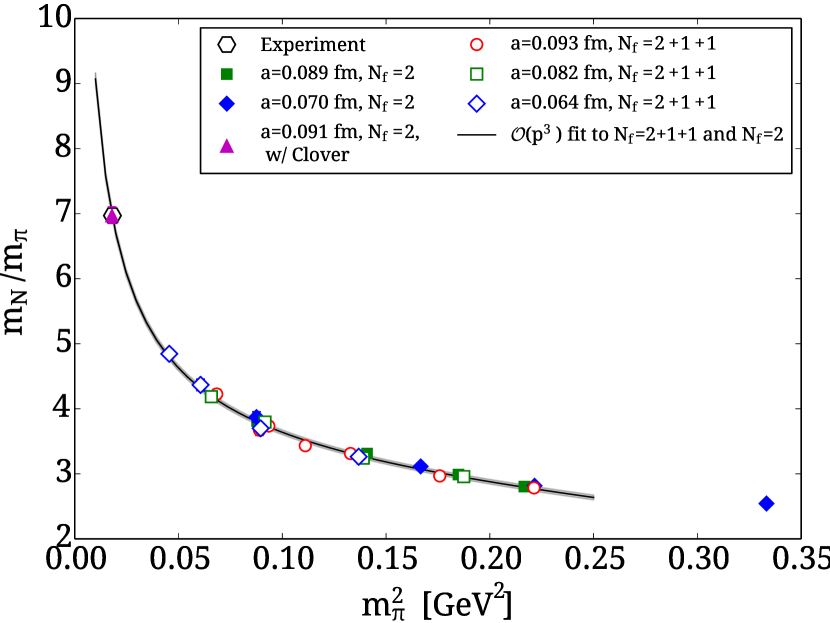
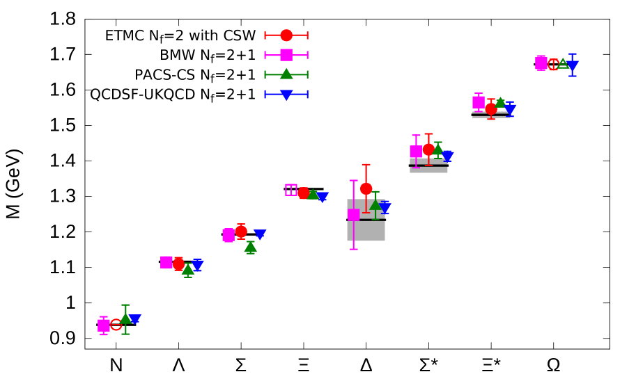
Figure 1: Left: Results on the ratio of the proton to the pion mass versus $m_{\pi}^{2}$ using TMF. The solid line is a leading oder chiral fit using $m_{\pi}<300$ MeV excluding the value at the physical point. Right: Lattice QCD results on the octet and decuplet baryon masses compared to the experimental values shown by the horizontal bands. Results by the ETM collaboration are shown in red circles for the physical point ensemble [11]. Also shown are results using clover fermions from BMW [12] (magenta squares), from PACS-CS [13] (green triangles), and from QCDSF-UKQCD [14] (blue inverted triangles). Open symbols show the baryon mass used as input to the calculations.

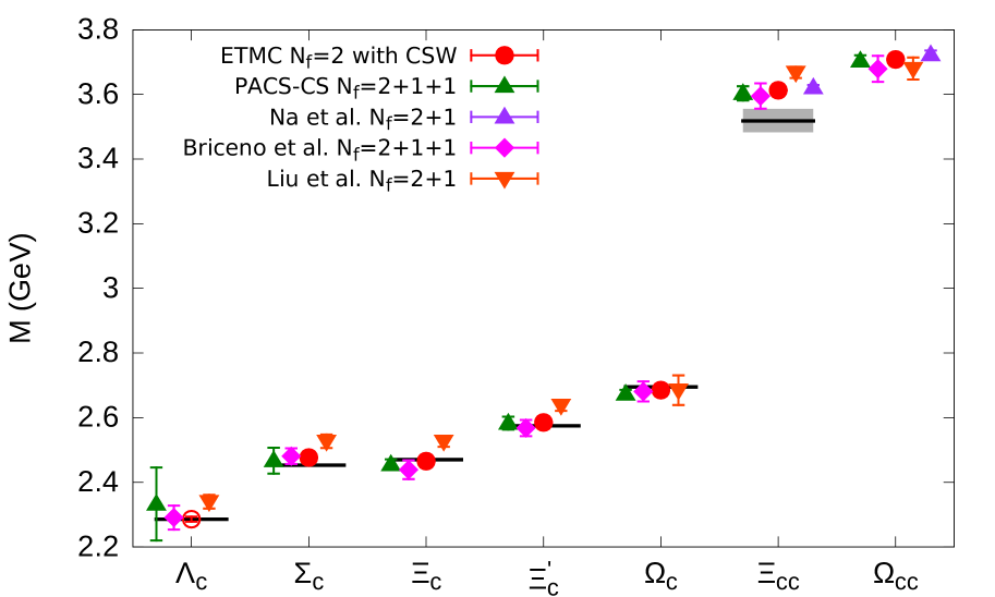
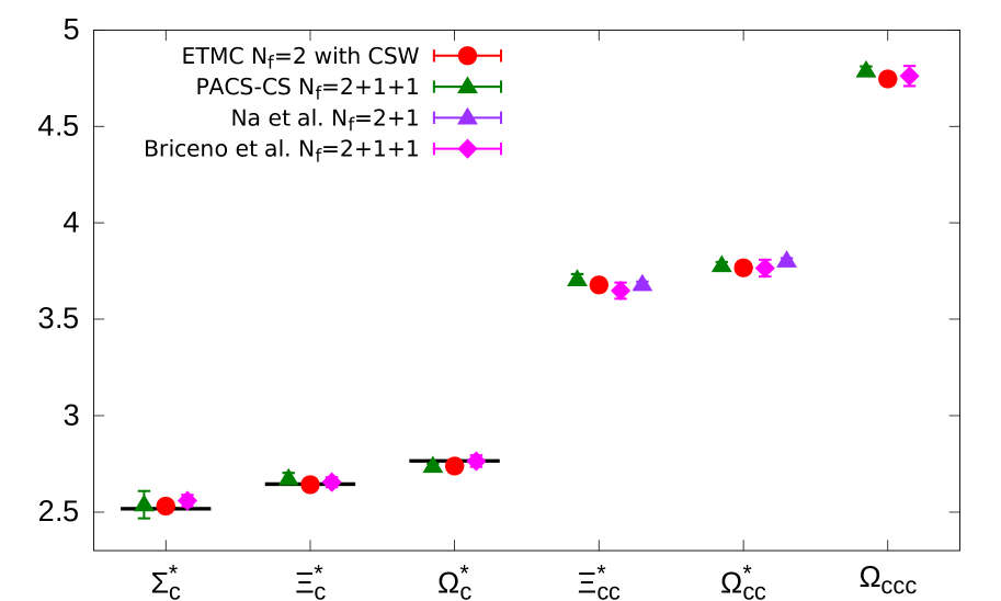
Figure 2: Results by ETMC are shown in red circles for the mass of the spin-$1/2$ (left) and spin-$3/2$ (right) charmed baryons for the physical point ensemble. Included are results from various hybrid actions with staggered sea quarks from Refs. [15] (purple triangles), [16] (magenta diamonds) and [17] (orange inverted triangles). Results from PACS-CS [18] are shown in green triangles.

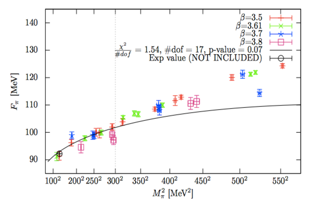
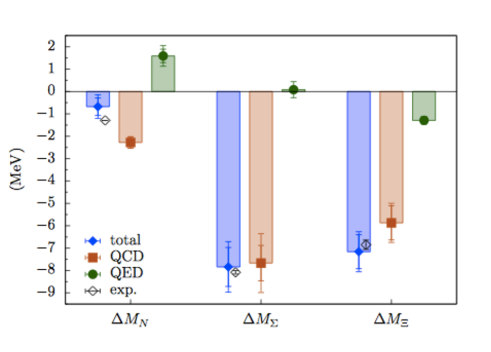
Figure 3: Left: Results on the pion decay constant $f_{\pi}$ by BMW. The solid line is the result of fitting NLO SU(2) chiral perturbation theory for $m_{\pi}<300$ MeV, taken from Ref. [7]. Right: Baryon spectrum with mass splitting by BMW taken from Ref. [21].

In Fig. 1 we show the ratio of the nucleon mass to the pion mass $m_{N}/m_{\pi}$ versus $m_{\pi}^{2}$ for a number of $N_{f}=2$ and $N_{F}=2+1+1$ TMF ensembles including the one with the physical point ensemble (with pion mass $m_{\pi}=130$ MeV, $a=0.094$ fm and $L=4.5$ fm) for which the dimensionless ratio $m_{N}/m_{\pi}$ agrees with its experimental value. In the same figure we also show results on the low-lying baryon spectrum from the ETM, BMW, PACS-CS and QCDSF-UKQCD collaborations. The set of TMF results shown in Fig. 1 is obtained using the physical point ensemble, thus requiring no chiral extrapolation, reducing drastically the systematic error that was found to be dominated by the chiral extrapolation in an earlier study using TMF [19]. These results are, however, obtained at one lattice spacing and volume. The analysis of Ref. [19] has shown that lattice artifacts both due to the finite volume and lattice spacing $a$ are small and thus the values obtained for the physical point ensemble are expected to have small lattice artifacts. This is indeed corroborated by the fact that the ’raw’ lattice data agree with the experimental values [11]. In Fig. 2 we show the corresponding results for the mass of the charmed baryons using the physical point ensemble in the case of TMF. As can be seen, the known values of the masses of the charmed baryons are reproduced and thus our computation provides a prediction for the yet unmeasured masses. Our preliminary values for the $\Xi_{cc}^{*}$ is 3.678(8) GeV, for the $\Omega^{+}_{cc}$ is 3.708(10) GeV, for $\Omega^{*+}_{cc}$ 3.767(11) GeV and for $\Omega^{++}_{ccc}$ 4.746(3) GeV.

The BMW collaboration has produced a number of ensembles using $N_{f}=2+1$ clover improved Wilson fermions with HEX smearing. They represent the most comprehensive set of ensembles for light pion masses close to and at the physical point. Their results on the pion decay constant $f_{\pi}$ are shown in Fig. 3. Fitting to NLO SU(2) chiral perturbation theory using pion masses up to 300 MeV they reproduce the physical value of $f_{\pi}$.

The BMW and QCDSF-UKQCD [20] collaborations investigated the mass splitting due to isospin breaking and electromagnetic effects. In Fig. 3 we show the results on the nucleon, $\Sigma$ and $\Xi$ baryons by the BMW collaboration [21] where isospin and electromagnetic effects were treated to lowest order. The agreement with the experimental values is a spectacular success of lattice QCD.

4 Challenges and future perspectives

The results shown in the previous section highlight the success of lattice QCD and the promise it holds to provide insight on many other observables. We will briefly discuss some of the challenges that need to be addressed in order for this to happen.

4.1 Excited states and resonances

In order to go beyond the low-lying spectrum one needs a formulation to extract excited states. The standard approach is to use a variational basis of interpolating fields to construct a correlation matrix of two-point functions:

$$G_{jk}(t_{s})=\langle{J_{j}(t_{s})J_{k}^{\dagger}(0)}\rangle\>,j,k=1,\ldots N$$ (3)

and then solve the generalized eigenvalue problem (GEVP) defined by

$$G(t)v_{k}(t;t_{0})=\lambda_{k}(t;t_{0})G(t_{0})v_{k}(t;t_{0})\rightarrow\lambda_{k}(t;t_{0})=e^{-E_{k}(t-t_{0})}\quad,$$ (4)

which yields the N lowest eigenstates.

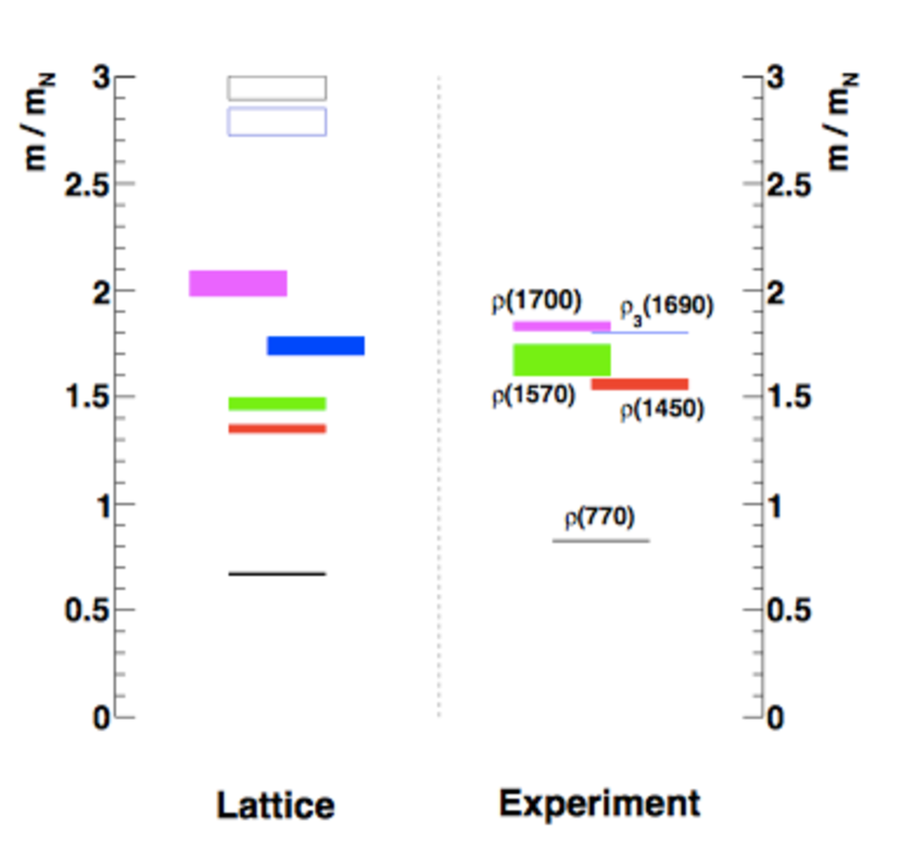
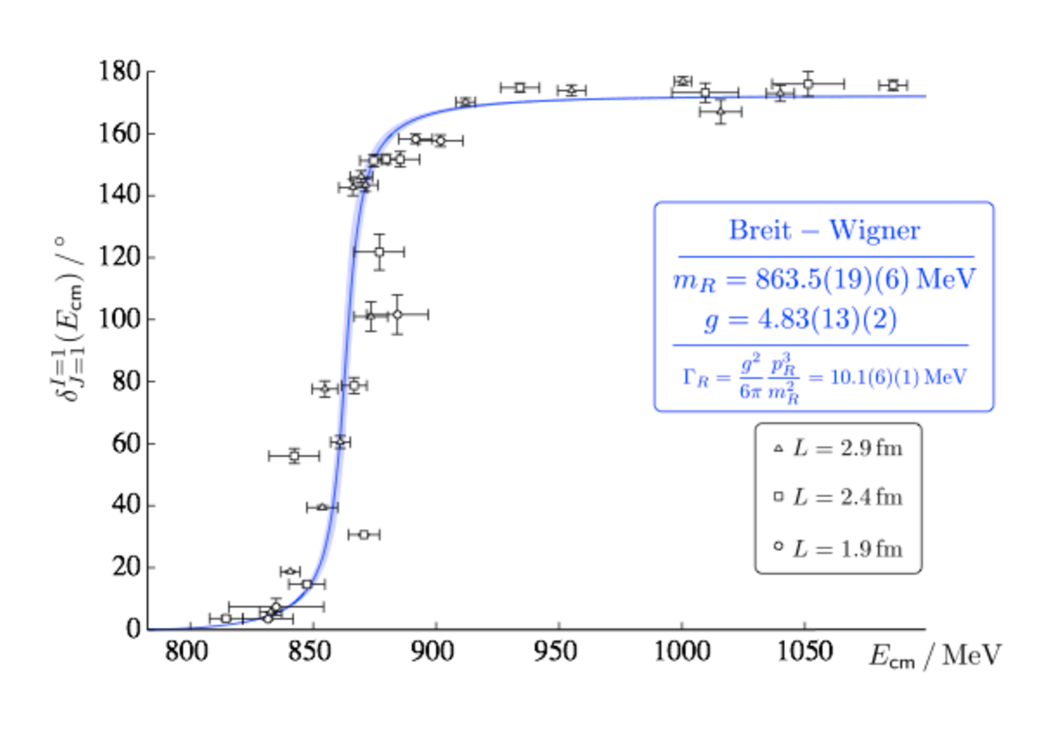
Figure 4: Left: Excited states of the $\rho$-meson at $m_{\pi}\sim 400$ MeV at one lattice spacing and one lattice volume, compared to experiment [22]. Right: The $\rho$-meson width, taken from Ref. [23].

A lot of effort has been devoted to construct appropriate bases using lattice symmetries by e.g. the Hadron Spectrum Collaboration. In order to determine the energy of an excited state one: i) must extract all states lying below the state of interest, ii) include disconnected diagrams, iii) treat appropriately resonances and unstable particles that require including multi-hadron states. Given the increased complexity of the problem it comes with no surprise that the calculations performed so far have not reached the maturity of ground state mass computations. In Fig. 4 we show results obtained on the $\rho$-meson excited spectrum [22] at $m_{\pi}=400$ MeV, as well as, on the width of the $\rho$-meson using using $N_{f}=2+1$ clover fermions and 3 asymmetric lattices [23]. These results, although still at larger than physical pion masses, provide a promising framework for the study of unstable particles.

4.2 Nucleon Structure

In order to evaluate hadron matrix elements one needs the appropriate three-point functions. There are two contributions we typically need to evaluate: the so called connected and disconnected parts, the former having the current coupled to a valence quark, while the later to a sea quark. Methods to evaluate the connected contribution are well developed see e.g. [24]. The disconnected contributions are much more demanding for technical reasons but also because they are prone to large gauge noise. Thus in most hadron structure computations they were neglected.

4.2.1 Axial charges

Some important nucleon observables only need the connected part. These are isovector quantities for which the disconnected contributions vanish in the isospin limit. The nucleon axial charge $g_{A}$ is extracted from the nucleon matrix element of the isovector axial-vector current and thus it is protected from disconnected contributions. It is also well-determined experimentally from $\beta$-decays and can be extracted directly at zero momentum transfer squared $q^{2}$ from $\langle N({\bf p}^{\prime})|j_{A}|N({\bf p})\rangle|_{q^{2}=0}$. It thus comprises an ideal benchmark quantity for lattice QCD.

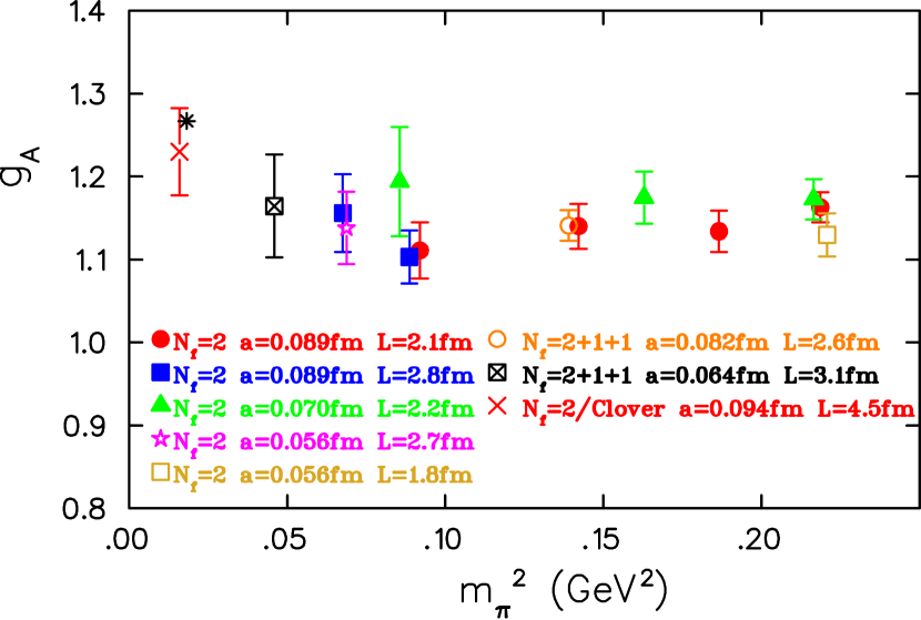
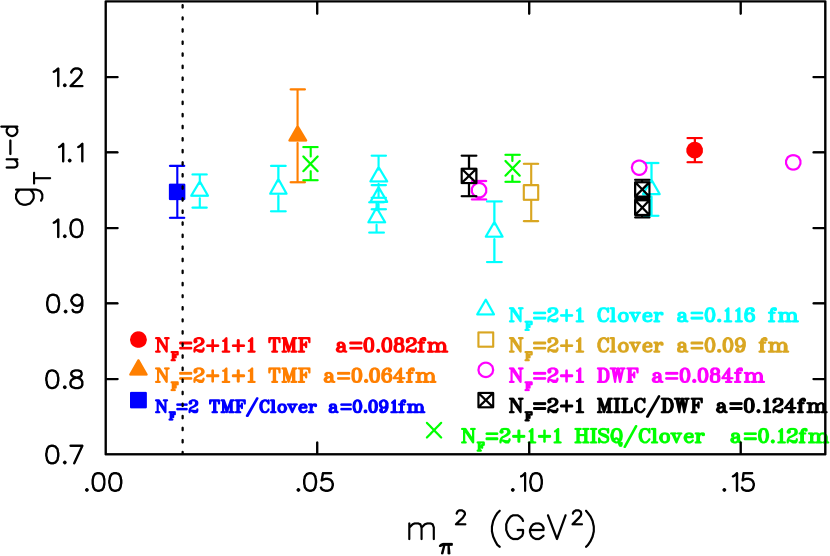
Figure 5: Left: Nucleon axial charge using TMF fermions. Right: Nucleon isovector tensor charge using TMF (ETMC) [25], DWF (RBC) [26], $N_{f}=2$ (QCDSF-UKQCD) [27] and $N_{f}=2+1$ (LHPC) [28] clover fermions, and clover on $N_{f}=2+1+1$ staggered (PNDME) [29].

We show in Fig. 5 results on the nucleon axial charge using the TMF ensembles. They are the ’raw’ lattice QCD data in the sense that they have not been volume corrected nor extrapolated to the continuum limit, but have been non-perturbatively renormalized. They are obtained by fitting to the plateau of an appropriately defined ratio of the three- to two-functions using a sink-source separation of about 1 fm. Within the current errors no dependence on the lattice spacing and volume is observed. While results at higher pion mass underestimate $g_{A}$, a fact observed by all lattice QCD collaborations, at the physical point we find a value that is in agreement with experiment. Despite the fact that the statistical error is still large, this is a very welcome result that would resolve a puzzle that persisted for some time showing the importance of computing observables at the physical point.

Having computed the axial charge it is straight forward to calculate the isovector scalar and tensor charges. The value of the latter is particularly relevant for searching for new type of interactions beyond the Standard Model. There is a planned SIDIS on ³He/Proton experiment to take place at JLab after the upgrade at 11 GeV. In lattice QCD it is computed by replacing the axial-vector current by the tensor current $j_{T}^{3}=\bar{\psi}(x)\sigma^{\mu\nu}\frac{\tau^{3}}{2}\psi(x)$. Studies have shown that $g^{u-d}_{T}$ has a similar behavior to $g_{A}$ as far as the contribution from excited states is concerned. We show results in Fig. 5 obtained using TMF, clover, DWF and in a mixed action set-up of staggered sea and clover valence quarks. As can seen, all lattice QCD results are in agreement and a preliminary value of $g_{T}^{u-d}=1.048(34)$ in $\overline{\rm MS}$ at 2 GeV is obtained from the TMF ensemble directly at the physical point.

4.2.2 Disconnected quark loop contributions

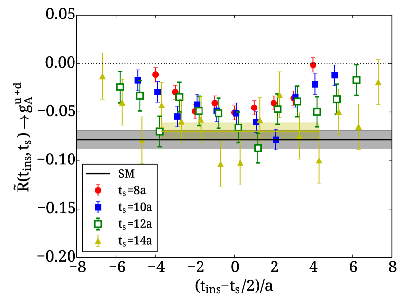
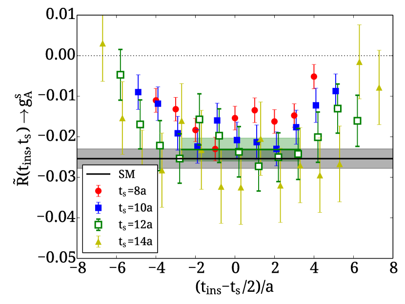
Figure 6: Disconnected contributions to the isoscalar (left) and strange (right) nucleon axial charge for the B55 ensemble.

Disconnected quark loop contributions arise from the coupling of the current to sea quarks. They are notoriously difficult to compute in lattice QCD. The technical reason is that one must compute a close quark loop given by $L(x)=Tr\left[\Gamma G(x;x)\right]\>$ for a general bilinear ultra-local operator of the form $\bar{\psi}(x)\Gamma\psi(x)$. This requires the computation of quark propagators from all ${\bf x}$ (all-to-all propagator) and thus it is $L^{3}$ more expensive as compared to the calculation of hadron masses. The other reason is that these loops tend to have large gauge noise and therefore large statistics are necessary to obtain a meaningful result. Special techniques that utilize stochastic noise on all spatial lattice sites are utilized in order to allow for the computation of the all-to-all propagator reducing the number of inversions to $N_{r}$ with $N_{r}\ll L^{3}$. The gauge noise is reduced by increasing statistics at low cost using low precision inversions and correcting for the bias (truncated solver method (TSM) or all-mode-averaging). Despite these new approaches the computation of these contributions would be too expensive using conventional computers. We take advantage of graphics cards (GPUs) for which we developed special multi-GPU codes. These computer architectures are ideal for approaches like TSM. We have illustrated the applicability of these methods by performing a high-statistics analysis using an $N_{f}=2+1+1$ TMF ensemble with $L=2.6$ fm, $a$ = 0.082 fm at $m_{\pi}$ = 373 MeV, referred to as the B55 ensemble. We analyzed 4700 gauge configurations yielding a total of ${\sim 150,000}$ statistics. The results on the disconnected contributions to the nucleon axial charge due to the light quarks $g^{u+d}_{A}$ and due to the strange $g^{s}_{A}$ are shown in Fig. 6. We obtain a non-zero negative value, which is ${\cal O}(10\%)$ for the u- and d-quarks and has to be taken into account when e.g. discussing the intrinsic spin $\frac{1}{2}\Delta\Sigma$ carried by quarks in the nucleon.

4.2.3 Electromagnetic form factors

The nucleon electromagnetic form factors are extracted from

$$\langle N(p^{\prime},s^{\prime})|j^{\mu}(0)|N(p,s)\rangle=\bar{u}_{N}(p^{\prime},s^{\prime})\left[\gamma^{\mu}{F_{1}(q^{2})}+\frac{i\sigma^{\mu\nu}q_{\nu}}{2m}{F_{2}(q^{2})}\right]u_{N}(p,s)\quad.$$ (5)

We would like to discuss here two studies at near physical pion mass: the one with the physical point ensemble of ETMC at $m_{\pi}=130$ MeV [30] and the one by LHPC using $N_{f}=2+1$ clover fermions configurations produced by the BMW collaboration with $a=0.116$ MeV and $m_{\pi}=149$ MeV [31].

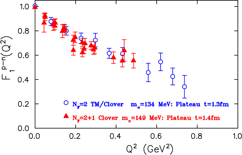
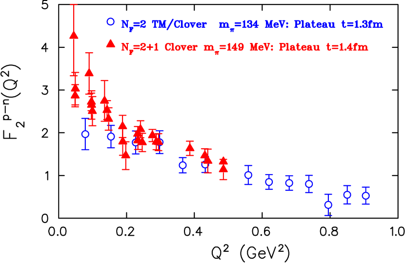
Figure 7: Results on the isovector Dirac (left) and Pauli (right) form factors versus $Q^{2}=-q^{2}$. The statistics is about $\sim 10^{3}$ for ETMC and 7750 for LHPC.

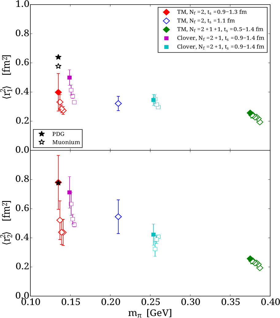
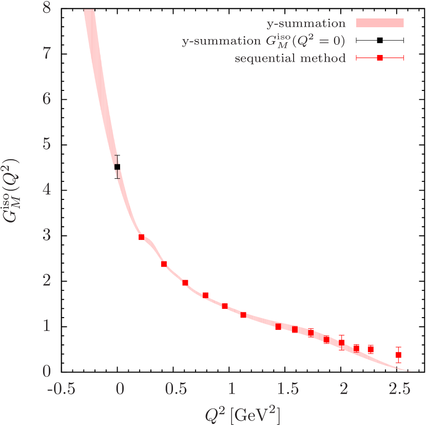
Figure 8: Left: Results on the isovector Dirac (top) and Pauli (bottom) radii versus $m_{\pi}^{2}$ from ETMC (diamonds) and LHPC (squares) [30]. Right: Magnetic form factor directly at $Q^{2}=0$, as determined by the red band [32]. The red points show the results with the conventional method.

Comparing the results on the Dirac and Pauli form factors between ETMC and LHPC in Fig. 7 we observe an overall agreement independently of the discretization scheme. The Dirac and Pauli radii can be extracted by fitting the $Q^{2}$-dependence of $F_{1}(Q^{2})$ and $F_{2}(Q^{2})$ to a dipole form, $\frac{A_{i}}{(1+Q^{2}/M_{i}^{2})^{2}}$, with $i=1,2,A_{1}=1$ and taking the derivative: $\langle r_{i}^{2}\rangle=-\frac{6}{F_{i}}\frac{dF_{i}}{dQ^{2}}|_{Q^{2}=0}=\frac{12}{M_{i}^{2}}$. The results are shown is Fig. 8 and clearly increase as the pion mass decreases, as well as the sink-source separation increases from $\sim 1$ fm to $\sim 1.3$ fm (see Ref. [30] for more details). However, fitting to a dipole to extract the radii introduces a model-dependence. We developed a novel method that extracts the value directly at $Q^{2}=0$. The first application of this method was to extract the anomalous magnetic moment determined by the magnetic form factor $G_{M}(0)$ or equivalently $F_{2}(0)$. In Fig. 8, our results on the isovector $G_{M}$ for the B55 ensemble are shown with the red band. As can be seen, the method provides a good determination of $G_{M}(0)$ without requiring any assumption of its $Q^{2}$-dependence (see Ref. [32] for more details).

5 Conclusions

Simulations at the physical point are now feasible and this opens exciting possibilities for the study of hadron structure. In this work we presented an overview of lattice QCD results obtained directly at or close to the physical point from a number of lattice QCD collaborations, such as results on the hyperon and charmed baryon masses and isospin splitting, the pion decay constant, as well as, on the axial and tensor charges, and electromagnetic form factors of the nucleon. We find a value of $g_{A}$ that is in agreement with experiment and provide a preliminary value for the tensor charge. The computation of disconnected contributions are briefly reviewed focusing on the disconnected quark contributions to the nucleon axial charge. First results at the physical point highlight the need for higher statistics in order that careful cross-checks can be carried out. Noise reduction techniques such as all-mode-averaging, improved methods for disconnected diagrams and smearing techniques are currently being pursued aiming at decreasing our errors on the quantities obtained at the physical point. When this is achieved, lattice QCD can provide reliable predictions on quantities probing beyond the standard model physics such as $g_{T}$, as well as, on the nucleon $\sigma$-terms.

6 Acknowledgments

I would like to thank the members of the ETMC and in particular my close collaborators A. Abdel-Rehim, M. Constantinou, K. Jansen, K. Hadjiyiannakou, C. Kallidonis, G. Koutsou, K. Ottnad, M. Petschlies and A. Vaquero for their contributions to the TMF results shown in this talk. Partial support was provided by the EU ITN project PITN-GA-2009-238353 (ITN STRONGnet) and IA project IA-GA-2011-283286 HadronPhysics3 . This work used computational resources provided by PRACE, JSC, Germany and the Cy-Tera project (NEA Y$\Pi$O$\Delta$OMH/$\Sigma$TPATH/0308/31).

7 Bibliography

References

- [1] , A. Abdel-Rehim et al. (ETMC), PoS(LATTICE2013) 264 (2013); A. Abdel-Rehim et al., (ETMC) PoS(LATTICE2014) 119 (2014).
- [2] C. Alexandrou et al., Comput. Phys. Commun. 185, 1370 (2014) [arXiv:1309.2256].
- [3] A. Abdel-Rehim et al., Phys. Rev. D 89, no. 3, 034501 (2014) [arXiv:1310.6339].
- [4] C. Alexandrou et al., PoS(LATTICE2014) 140 (2014).
- [5] S. Meinel et al., PoS(LATTICE2014) 139 (2014).
- [6] A. Bazavov et al. [Fermilab Lattice and MILC Collaboration], arXiv:1407.3772 [hep-lat].
- [7] S. Durr et al., arXiv:1310.3626 [hep-lat].
- [8] G. S. Bali et al., Nucl. Phys. B 866, 1 (2013).
- [9] S. Aoki et al. [PACS-CS Collaboration], Phys. Rev. D 81, 074503 (2010).
- [10] S. Syritsyn et al., (RBC/UKQCD) PoS(LATTICE2014) 134 (2014).
- [11] C. Alexandrou et al., PoS(LATTICE2014) 151 (2014).
- [12] S. Durr et al. Science 322, 1224 (2008).
- [13] S. Aoki et al. [PACS-CS Collaboration], Phys. Rev. D 79, 034503 (2009).
- [14] W. Bietenholz et al., Phys. Rev. D 84, 054509 (2011).
- [15] H. Na and S. A. Gottlieb, PoS LAT 2007, 124 (2007); H. Na and S. Gottlieb, PoS LATTICE 2008, 119 (2008).
- [16] R. A. Briceno, H. W. Lin and D. R. Bolton, Phys. Rev. D 86, 094504 (2012).
- [17] L. Liu, H. W. Lin, K. Orginos and A. Walker-Loud, Phys. Rev. D 81, 094505 (2010).
- [18] Y. Namekawa et al. [PACS-CS Collaboration], Phys. Rev. D 87, 094512 (2013).
- [19] C. Alexandrou, V. Drach, K. Jansen, C. Kallidonis and G. Koutsou, arXiv:1406.4310 [hep-lat].
- [20] R. Horsley et al. (QCDSF-UKQCD) Phys. Rev. D 86, 114511 (2012); PoS Lattice 2013, 499 (2013).
- [21] Sz. Borsanyi et al., Phys. Rev. Lett. 111 (2013) 252001.
- [22] J. Bulava et al., [arXiv:1310.7887[hep-lat]].
- [23] J. J. Dudek, R. G. Edwards and C.E. Thomas, Phys. Rev. D 87 (2013) 034505.
- [24] C. Alexandrou, Prog. Part. Nucl. Phys. 67, 101 (2012) [arXiv:1111.5960 [hep-lat]].
- [25] C. Alexandrou, M. Constantinou, K. Jansen, G. Koutsou and H. Panagopoulos, arXiv:1311.4670 [hep-lat].
- [26] Y. Aoki et al., Phys. Rev. D 82, 014501 (2010).
- [27] D. Pleiter et al. [QCDSF/UKQCD], PoS LATTICE 2010, 153 (2010) [arXiv:1101.2326 [hep-lat]].
- [28] J. R. Green et al., Phys. Rev. D 86, 114509 (2012).
- [29] T. Bhattacharya et al., Phys. Rev. D 89, 094502 (2014).
- [30] C. Alexandrou et al. (ETMC), PoS (LATTICE2014) 148 (2014).
- [31] J. R. Green et al., Phys. Rev. D 90, 074507 (2014).
- [32] C. Alexandrou et al. (ETMC), PoS (LATTICE2014) 144 (2014).