Efficient simulation of semiflexible polymers

Abstract

Using a recently developed bead-spring model for semiflexible polymers that takes into account their natural extensibility, we report an efficient algorithm to simulate the dynamics for polymers like double-stranded DNA (dsDNA) in the absence of hydrodynamic interactions. The dsDNA is modelled with one bead-spring element per basepair, and the polymer dynamics is described by the Langevin equation. The key to efficiency is that we describe the equations of motion for the polymer in terms of the amplitudes of the polymer’s fluctuation modes, as opposed to the use of the physical positions of the beads. We show that, within an accuracy tolerance level of $5\%$ of several key observables, the model allows for single Langevin time steps of $\approx 1.6$, 8, 16 and 16 ps for a dsDNA model-chain consisting of 64, 128, 256 and 512 basepairs (i.e., chains of 0.55, 1.11, 2.24 and 4.48 persistence lengths) respectively. Correspondingly, in one hour, a standard desktop computer can simulate 0.23, 0.56, 0.56 and 0.26 ms of these dsDNA chains respectively. We compare our results to those obtained from other methods, in particular, the (inextensible discretised) WLC model. Importantly, we demonstrate that at the same level of discretisation, i.e., when each discretisation element is one basepair long, our algorithm gains about 5-6 orders of magnitude in the size of time steps over the inextensible WLC model. Further, we show that our model can be mapped one-on-one to a discretised version of the extensible WLC model; implying that the speed-up we achieve in our model must hold equally well for the latter. We also demonstrate the use of the method by simulating efficiently the tumbling behaviour of a dsDNA segment in a shear flow.

I Introduction

Over the last decades, there has been a surge in research activities in the physical properties of biopolymers, such as double-stranded DNA (dsDNA), filamental actin (F-actin) and microtubules. Semiflexibility is a common feature they share: they preserve mechanical rigidity over a range, characterised by the persistence length $l_{p}$, along their contour. (E.g., for a dsDNA, F-actin and microtubules, $l_{p}\approx 40$ nm dnapersist ; wang , $\sim 16\mu$m Factinpersist and $\sim 5$ mm micropersist respectively.)

Recently, two of us introduced a bead-spring model for semiflexible polymers leeuwen . The model has four parameters. Three of them determine the mechanical properties: the average inter-bead distance $a$, the longitudinal stiffness $\lambda$, and the bending stiffness $\kappa$. The fourth parameter is related to the viscosity of water $\xi$ and sets the time scale. In earlier work leeuwen ; leeuwen1 we determined a set of values for the first three parameters that are able to reproduce the mechanical properties of double-stranded DNA in experiment, and we studied the canonical averages of a number of equilibrium properties. In most of the present paper, we restrict ourselves to the same set of parameter values.

In this paper, we primarily discuss how the equations of motion of our model can be efficiently integrated in time. There is no hydrodynamic interactions among the beads. This is in fact not a problem when it comes to comparing to experimental results for dsDNA segments up to a few persistence lengths, since at these lengths a semiflexible polymer does not form a coil, and therefore should be free-draining. Indeed, this is the feature that allows us to meaningfully compare the diffusion coefficients of short model dsDNA segments to those from experiments, from which we determine the fourth (and the last) parameter of the model, $\xi$, which describes the Langevin friction on the beads.

The default simulation approach to integrate the corresponding Langevin equations of motion in time for our model would be a simple integration scheme such as the Euler method, using the bead positions as dynamical variables. In this paper we develop a time-forward integration scheme by using the properties of (a very good approximation of) the polymer’s fluctuation modes in this model leeuwen1 , and allowing a set of representative equilibrium and dynamical observables to differ by at most 5%, we achieve 2-3 orders of magnitude speed-ups in comparison to the default method. With average inter-bead distance $a\approx 0.33$ nm as a model parameter, the length of a dsDNA basepair, the maximum size $\Delta t_{\text{max}}$ of the time step is summarised in Table 1.

chain length (bp)	$\quad\Delta t_{\text{max}}$ (ps)
64	1.59
128	7.96
256	15.9
512	15.9

Table 1: With average inter-bead distance $a\approx 0.33$ nm — the length of a dsDNA basepair — as a model parameter, the maximum size of the integration time step $\Delta t_{\text{max}}$ are shown for various chain lengths for dsDNA. The persistence length we use is $l_{p}\approx 37.6$ nm wang , corresponding to $\approx 114$ basepairs.

We also relate our work to existing theoretical work on semiflexible polymers. We show that our model can be mapped one-on-one to the discretised version of the extensible wormlike chain (WLC) model ober ; implying that the speed-up we achieve in our model must hold equally well for the latter. We further demonstrate that if in our model the longitudinal stiffness $\lambda$ is made very large while keeping fixed its resistance to bending $\kappa$, it effectively reduces to a discretised version of the inextensible WLC model kratky . (The inextensible WLC model, its subsequent modifications mods1 ; mods2 ; mods3 ; mods4 , and recent analyses recent1 ; recent2 ; recent3 ; recent4 ; recent5 ; recent6 have been very successful in describing static/mechanical properties of dsDNA, such as its force-extension curve and the radial distribution function of its end-to-end distance.) Since the contour length of the polymer is constrained in the original inextensible WLC model, Lagrangian multipliers of a varying degree of sophistication have been introduced in its computer implementation in order to enforce a contour length that is either strictly fixed liverpool1 ; liverpool2 ; liverpool3 ; liverpool4 ; kroy ; morse ; montesi , or fixed on average winkler1 ; winkler2 . In particular, we show that in the limit of large $\lambda$ at fixed $\kappa$ the dynamical equations of the beads in our model approach those similar to the ones that Morse morse ; montesi developed in order to simulate the inextensible WLC. Using this relation between our model and the inextensible WLC, we demonstrate that the maximal allowable time step $\Delta t_{\text{max}}$ for the inextensible WLC model of a dsDNA chain of 63 basepairs is $\approx 0.02$ fs, in good agreement with Ref. frey (that has recently implemented Morse’s algorithm for the inextensible WLC). In other words, as shown in Table 1, to simulate dsDNA our model achieves a maximal allowable time step that is 5-6 orders of magnitude larger than that of the inextensible WLC.

This paper is organised as follows. In Sec. II we briefly introduce the model, and identify the parameter values of the model Hamiltonian for dsDNA. Here we also show that our model, in the parameter space, can be mapped one-on-one to the discretised version of the extensible WLC model. In Sec. III we describe the equations for polymer dynamics. Section IV is devoted to the time-integrated algorithm for the equation of motion for the polymer in mode representation. In Sec. V we test the time-integration algorithm for dsDNA. In Sec. VI we discuss coarse-graining in our model, which leads us to the result that in the limit of large $\lambda$ at fixed $\kappa$ the dynamical equations of the beads in our model approach those similar to the ones that Morse morse ; montesi developed in order to simulate the inextensible WLC. In Sec. VII we elaborate on our numerical results presented in Table 1, and we conclude the paper with a discussion in Sec. VIII, including a wider comparison to the time steps achieved in the existing literature. Finally, in the Supplementary Information we present a movie of a tumbling dsDNA segment in a shear flow, generated by the use of this algorithm, to illustrate the usefulness of the simulation approach.

II The model

The model we use for semiflexible polymers is described in detail in Ref. leeuwen . The Hamiltonian for the model is of the form

$${\cal H}=\frac{\lambda}{2}\sum^{N}_{n=1}(|{\bf u}_{n}|-d)^{2}-\kappa\sum^{N-1}_{n=1}{\bf u}_{n}\cdot{\bf u}_{n+1}.$$ (1)

Here ${\bf u}_{n}={\bf r}_{n}-{\bf r}_{n-1}$ is the bond vector between bead $n-1$ and $n$, with ${\bf r}_{n}$ being the position of the $n$-th bead ($n=0,1,\cdots,N$). The first term in this Hamiltonian relates to the longitudinal stiffness of the chain, while the second term relates to its resistance to bending. The parameters in the Hamiltonian are the following. The quantity $d$ sets the length scale of a bond — if only the first term would be present, bonds would assume the length $d$. The presence of the second term in the Hamiltonian causes an elongation of the bonds such that the average bond length is $a=bd$, with a factor $b$ that depends on the type of the polymer. Further, $\lambda$ and $\kappa$ are two parameters, relating to the longitudinal (stretching) and transverse (bending) stiffness of the chain. In order to have ${\cal H}$ represent semiflexible polymers, both parameters $\lambda$ and $\kappa$ typically will have to be large. Instead of working in terms of $\lambda$ and $\kappa$, we choose the ratios $\nu=\kappa/\lambda$ and $T^{*}=k_{B}T/(\lambda d^{2})$ as characteristic parameters to describe the model leeuwen , which reduces the Hamiltonian to

$$\frac{\cal H}{k_{B}T}=\frac{1}{2T^{*}}\left[\sum^{N}_{n=1}(u_{n}-1)^{2}-2\nu\sum^{N-1}_{n=1}{\bf u}_{n}\cdot{\bf u}_{n+1}\right],$$ (2)

with $u_{n}\equiv\left|{\bf u}_{n}\right|$ is the length of the scaled bond vector. Note that stability of the Hamiltonian requires $0<\nu<1/2$, and that in these variables leeuwen ; leeuwen1

$$b=\frac{1}{1-2\nu}\quad\mbox{and}\quad l_{p}=\frac{ab^{2}\nu}{T^{*}}=\frac{\kappa a^{3}}{k_{B}T}.$$ (3)

II.1 The model parameters for dsDNA

For dsDNA the physical distance between the beads equals $a=0.33$ nm, i.e. the length of a basepair. The two parameters $T^{*}$ and $\nu$ can be chosen by matching the force-extension curve for the polymer, leading to $\nu=0.35$ and $T^{*}=0.034$ leeuwen . Following Eq.(3), the factor $b$ then turns out to be $\approx 3.3$, so that the length parameter $d\approx 0.1$ nm. The number of beads $(N+1)$ simply equals the number of basepairs present in the dsDNA chain.

The equilibrium and the dynamical properties of the model, specially in relation to the well-known properties of semiflexible polymers have been studied in detail in Refs. leeuwen ; leeuwen1 . Nevertheless, in order to demonstrate the usability of this model for reaching long length and time-scales on a computer we need to revisit the dynamical equations resulting from the Hamiltonian (2).

II.2 Relating our model to the extensible WLC

We start with the expression for the extensible WLC as given by Obermayer and Frey ober

$${\cal H}=\frac{k_{B}T}{2}\int^{L}_{0}ds\left(l_{p}\,|{\bf r}^{\prime\prime}|^{2}+k_{x}\,[|{\bf r}^{\prime}|-1]^{2}\right),$$ (4)

where ${\bf r}(s)$ is the contour of the chain, ${\bf r}^{\prime}$ the first derivative and ${\bf r}^{\prime\prime}$ the second derivative with respect to the contour length parameter $s$. In order to simulate the dynamical behaviour of the continuous chain, the chain is represented by a set of $N$ discrete points

$$s_{n}=n\Delta s,\quad\quad\quad L=N\Delta s,\quad\quad\quad{\bf r}_{n}={\bf r}(s_{n}).$$ (5)

The derivatives are replaced by

$${\bf r}^{\prime}\Rightarrow\frac{{\bf r}_{n}-{\bf r}_{n-1}}{\Delta s}=\frac{{\bf u}_{n}}{\Delta s},$$ (6)

and

$${\bf r}^{\prime\prime}\Rightarrow\frac{{\bf u}_{n+1}-{\bf u}_{n}}{\Delta s}=\frac{{\bf r}_{n+1}-2{\bf r}_{n}+{\bf r}_{n-1}}{(\Delta s)^{2}}$$ (7)

The points on the chain will correspond to the beads of our Hamiltonian. We take $\Delta s=a$ as the distance between the points for a transparent comparison between the models.

Inserting these derivatives into the Hamiltonian (4) yields

$${\cal H}=\frac{k_{B}T}{2a}\sum^{N}_{n=1}\left(l_{p}|{\bf u}_{n+1}-{\bf u}_{n}|^{2}+k_{x}[u_{n}-a]^{2}\right).$$ (8)

Writing out the squares and collecting the terms of the same nature we get

$${\cal H}=\frac{k_{B}T}{2a}\sum_{n}\left([2l_{p}+k_{x}]u^{2}_{n}-2l_{p}{\bf u}_{n}\cdot{\bf u}_{n+1}-2k_{x}a\,u_{n}\right).$$ (9)

We have left out the irrelevant constant and ignored the minor difference between the coefficient of first and last bond in the term with $u^{2}_{n}$ and those of the other bonds.

In order to compare the expression (9) with our Hamiltonian (1) we must realise that the Hamiltonian (4) uses a scaling that is not the same as ours. So there is an overall constant $f$ difference between the two Hamiltonians. Keeping this in mind we get the relations

$$f\,\frac{k_{b}T}{a}l_{p}=\kappa,\quad\quad f\,\frac{k_{b}T}{2a}(2l_{p}+k_{x})=\lambda,\quad\quad f\,k_{b}T\,k_{x}=\lambda d.$$ (10)

The overall factor $f$ is determined from the second relation (3) between the persistence length $l_{p}$ and our constant $\kappa$. The first relation (10) yields

$$f=1/a^{2}.$$ (11)

Using this in the last relation of Eq. (10) we get the connection between $k_{x}$ and $\lambda$.

$$k_{x}=\frac{\lambda da^{2}}{k_{B}T}.$$ (12)

Inserting Eqs. (3) and (12) into the middle relation of Eq. (10) leads to the relation

$$2\kappa+\frac{\lambda d}{a}=\lambda,\quad\quad{\rm or}\quad\quad\frac{d}{a}=\frac{1}{b}=1-2\nu,$$ (13)

which is consistent with the first relation (3).

Thus the discretised extensible WLC is identical to our model with the above given connection of the parameters, except for a small difference for the strength of the interaction parameters of the first and last bond. This implies that any conclusion we draw on our model is equally valid for discretised versions of the extensible WLC.

III Polymer dynamics

We describe the polymer dynamics in terms of the Langevin equation. It is natural to choose the positions of the beads as the dynamical variables, obeying the equations

$$\frac{d{\bf r}_{n}(t)}{dt}=-\frac{1}{\xi}\frac{\partial{\cal H}}{\partial{\bf r}_{n}}+{\bf g}_{n}(t).$$ (14)

Here $\xi$ is the friction coefficient and ${\bf g}_{n}$ is the Gaussian distributed random thermal force on bead $n$ due to the solvent molecules, with the fluctuation spectrum

$$\langle g^{\alpha}_{m}(t)\,g^{\beta}_{n}(t^{\prime})\rangle=\frac{2k_{B}T}{\xi}\,\delta^{\alpha,\beta}\,\delta_{m,n}\,\delta(t-t^{\prime}).$$ (15)

For numerical evaluation of these equations it is useful to reduce time and distances to dimensionless variables. We therefore scale distances and time by $d$ and time by $\xi/\lambda$, i.e., we write the bead positions as ${\bf r}_{n}={\bf r}^{\prime}_{n}d$ and $t=\xi\tau/\lambda$, which gives the Langevin equation the form

$$\frac{d{\bf r}^{\prime}_{n}(t)}{d\tau}=-\frac{\partial{\cal H}^{\prime}}{\partial{\bf r}^{\prime}_{n}}+{\bf g}^{\prime}_{n}(\tau).$$ (16)

Correspondingly, the dimensionless random force

$${\bf g}^{\prime}_{n}=\frac{{\bf g}_{n}d}{\lambda}$$ (17)

has the correlation function

$$\langle g^{\prime\alpha}_{m}(\tau)\,g^{\prime\beta}_{n}(\tau^{\prime})\rangle={2T^{*}}\,\delta^{\alpha,\beta}\,\delta_{m,n}\,\delta(\tau-\tau^{\prime}).$$ (18)

In order to restore notational simplicity henceforth we omit the primes on the variables.

III.1 The dynamical equations in terms of polymer’s fluctuation modes

It is of course possible to simulate polymer dynamics using the default Euler method, Eqs. (16-18), with the bead positions as variables. This however only allows Langevin time step $\Delta\tau=0.1$, and at $\Delta\tau\approx 0.3$ (corresponding to 0.16 and 0.48 ps respectively — $\Delta\tau=1$ corresponds to 1.5 ps, see Sec. VII.2) the integration scheme even becomes unstable. An equivalent manner to simulate polymer dynamics is to use its fluctuation modes as variables. The main advantage of the latter is that the modes with longer length-scales have slower decay times, and as result one can make a separation in time scales, which in turn allows for the possibility of larger time steps, i.e., faster simulations that eventually achieves 2-3 orders of magnitude larger integration time steps. In this section we describe the method.

As for describing polymer dynamics in terms of the polymer’s fluctuation modes (described by the mode variables ${\bf R}_{p}$), note that any transformation of the type

$$\left\{\begin{array}[]{rcl}{\bf R}_{p}&=&\displaystyle\sum_{n}{\bf r}_{n}\,\phi_{n,p},\\[11.38109pt] {\bf r}_{n}&=&\displaystyle\sum_{p}\phi_{n,p}\,{\bf R}_{p},\end{array}\right.$$ (21)

where $\phi_{n,p}$ is an orthogonal matrix, satisfying

$$\sum_{p}\phi_{m,p}\,\phi_{n,p}=\delta_{mn},$$ (22)

leaves the dynamical equation (16) form invariant; i.e.,

$$\frac{d{\bf R}_{p}(t)}{d\tau}=-\frac{\partial{\cal H}}{\partial{\bf R}_{p}}+{\bf G}_{p}.$$ (23)

Here ${\bf G}_{p}$ is the transform of ${\bf g}_{n}$:

$${\bf G}_{p}=\sum_{n}{\bf g}_{n}\,\phi_{n,p},$$ (24)

whereas the derivative with respect to ${\bf R}_{p}$ can be calculated with the chain rule

$$\frac{\partial{\cal H}}{\partial{\bf R}_{p}}=\sum_{n}\frac{\partial{\cal H}}{\partial{\bf r}_{n}}\phi_{n,p}.$$ (25)

Returning to our Hamiltonian (2), we see that it can be rewritten in the form leeuwen

$$\frac{{\cal H}}{k_{B}T}-N/2=\frac{1}{2}\sum_{m,n}{\bf r}_{m}\cdot H_{m,n}{\bf r}_{n}-L_{c}={\cal H}^{*}-L_{c},$$ (26)

with $L_{c}$ the contour length

$$L_{c}=\sum_{n}u_{n}.$$ (27)

In this form of the Hamiltonian, the ${\cal H}^{*}$ term is not only quadratic in the bead positions, but also $H_{mn}$ becomes diagonal under the transformation ($p=0,1,\ldots,N-1$) leeuwen

$$\phi_{n,p}=\left(\frac{2}{N+1}\right)^{1/2}\,\cos\left(\frac{p(n+1/2)\pi}{N+1}\right),$$ (28)

which are of the same form as the Rouse modes for a flexible polymer rouse , with eigenvalues

$$\zeta^{l}_{p}=2\left[1-\cos\left(\frac{p\pi}{N+1}\right)\right]\left[1-2\nu\cos\left(\frac{p\pi}{N+1}\right)\right].$$ (29)

In other words, ${\cal H}^{*}$ is simply expressed as

$${\cal H}^{*}=\frac{1}{2}\sum_{p}\zeta^{l}_{p}R^{2}_{p}.$$ (30)

Unfortunately though, the term $L_{c}$ in the Hamiltonian (26) is not diagonal in the Rouse mode representation, meaning that $L_{c}$ contains coupling among different Rouse modes. Consequently, the equation of motion for the polymer takes the form

$$\frac{d{\bf R}_{p}(t)}{d\tau}=-\zeta_{p}^{l}{\bf R}_{p}+{\bf H}_{p}+{\bf G}_{p},$$ (31)

where ${\bf H}_{p}=-\partial{L_{c}}/\partial{\bf R}_{p}$. In this form it becomes clear that the times scales for the modes, given by $(\zeta^{l}_{p})^{-1}$, vary widely with the mode index $p$, ranging from large for small $p$ to small for $p$ of the order $N$. In the next sections, by separating the time-scales in this manner, that the important physics is contained in the low modes and that treating them correctly opens up a window of opportunity to take large time steps in the numerical integration of Eq. (23).

Having said the above, we also note that the choice of the Rouse modes in representing the dynamical equation is by no means unique. An equivalent representation in terms of the polymer’s fluctuation modes, well-elaborated in one of our own publications leeuwen1 is as follows. In terms of the bead positions ${\bf r}_{n}$ of the chain one can expand the Hamiltonian around its ground state, which has a configuration of a straight rod. The second term in this expansion, involving the Hessian $\partial^{2}{\cal H}/\partial{\bf r}_{m}\partial{\bf r}_{n}$, is also quadratic in the bead positions, but it includes not only ${\cal H}^{*}$, but also some contribution from $L_{c}$. Indeed, as shown in Ref. leeuwen1 , the corresponding modes then yield the well-known transverse (bending) and longitudinal (stretching) modes of a semiflexible chain, with eigenvalues $\zeta^{t}_{p}$ and $\zeta^{l}_{p}$ respectively. [Of these, the longitudinal modes are identical to the Rouse modes (28-29), which explains our choice of notation for the eigenvalue in Eq. (29).] Thus, an equivalent, and perhaps more natural, choice of representing the dynamical equation (23) would be to use the longitudinal and the transverse modes. Our experience, however, is that using the Rouse mode representation makes the code faster and more robust for parameters $T^{*}$ and $\nu$ typical for dsDNA, to which we stick to in the rest of this paper (and also in our earlier publication leeuwen1 ).

IV Time-integrated algorithm for the equation of motion for the polymer in mode representation

We start with the (obvious) statement that without the coupling term ${\bf H}_{p}$, the integration of the equations (31) is straightforward. Each mode develops as an Ornstein-Uhlenbeck process, which admits an exact solution. As this is the basis of our refinements of the algorithm, we illustrate our method of time-integration of the equation of motion for the polymer by considering one scalar mode $R(t)$ with decay coefficient $\zeta$, a coupling force $H(t)$ and random force $G(t)$. It is useful to first make the substitution (c.f. the interaction representation in quantum mechanics)

$$R(t)=\exp(-\zeta t)\,\tilde{R}(t),$$ (32)

leading to the equation for $\tilde{R}(t)$

$$\frac{d\tilde{R}(t)}{dt}=[H(t)+G(t)]\,\exp(\zeta t).$$ (33)

Integrating this equation over a finite time interval $\Delta t$ and multiplying the result with $\exp(-\zeta\Delta t)$ then yields

$$R(t+\Delta t)=\exp(-\zeta\Delta t)\,R(t)+\overline{H}(t)+\overline{G}(t),$$ (34)

where $\overline{G}$ is given by

$$\overline{G}(t)=\int^{\Delta t}_{0}dt^{\prime}\,\exp[\zeta(t^{\prime}-\Delta t)]\,G(t+t^{\prime}),$$ (35)

and likewise, $\overline{H}$ is given by

$$\overline{H}(t)=\int^{\Delta t}_{0}dt^{\prime}\,\exp[\zeta(t^{\prime}-\Delta t)]\,H(t+t^{\prime}).$$ (36)

The distribution of $\overline{G}(t)$ is, as an integral (sum) over independent Gaussian random variables, i.e., a Gaussian random variable with variance

$$w^{2}(\Delta t)=T^{*}[1-\exp(-2\zeta\Delta t)]/\zeta;$$ (37)

i.e., in formula (35) the distribution reads

$$P(\overline{G})=\frac{1}{\sqrt{\pi}w(\Delta t)}\exp\left(-\frac{\overline{G}^{2}}{2w^{2}(\Delta t)}\right).$$ (38)

Note here that Equation (34) is an exact substitute for the Langevin equation with an arbitrary time step.

From the above one sees that the use of the polymer’s fluctuation modes to time-integrate the equation of motion has two aspects:

• If we manage to make $H$ small, we may treat the modes to be evolving independently, with only a small perturbation due to the coupling.

• We need to find an expression for the integral $\overline{H}(t)$, while we only have an expression for the initial value $H(t)$.

Clearly, the more successful we are with point (i), the less severe point (ii) becomes.

IV.1 A more functional form of ${\bf H}_{p}$ for polymer dynamics

The expression for ${\bf H_{p}}$ follows from Eqs. (26) and (29)

$${\bf H}_{p}=\frac{\partial L_{c}}{\partial{\bf R}_{p}}=\sum_{n}\,\frac{\partial L_{c}}{\partial{\bf r}_{n}}\phi_{n,p}=\sum_{n}\,[\hat{\bf u}_{n}-\hat{\bf u}_{n+1}]\,\phi_{n,p},$$ (39)

where $\hat{\bf u}_{n}={\bf u}_{n}/u_{n}$, is the unit bond vector, and $u_{n}=|{\bf u}_{n}|$. By rearranging the summation variable $n$ we write

$${\bf H}_{p}=\sum^{N}_{n=1}\hat{\bf u}_{n}\,\chi_{n,p},$$ (40)

with

$$\chi_{n,p}=\phi_{n,p}-\phi_{n-1,p}=2\left(\frac{2}{N+1}\right)^{1/2}\sin\left(\frac{p\pi}{2(N+1)}\right)\,\sin\left(\frac{pn\pi}{N+1}\right).$$

(41)

Using the bond-length factor $b$ introduced in (3), it is natural to write

$$\hat{\bf u}_{n}={\bf u}_{n}/b+\Delta\hat{\bf u}_{n}=(1-2\nu){\bf u}_{n}+\Delta\hat{\bf u}_{n}.$$ (42)

Inherent to Eq. (42) is the build-up of the following approximation scheme, as we demonstrate below. In the limit of small $T^{*}$ (i.e., high $\lambda$) — e.g., $T^{*}=0.034$ for dsDNA — the chain does not stretch much, hence we expect $\Delta\hat{\bf u}_{n}$ to be much smaller than ${\bf u}_{n}/b$; in other words, setting $\Delta\hat{\bf u}_{n}$ to zero provides a rather good approximation for $\hat{\bf u}_{n}$. Further, since ${\bf u}_{n}$ can be expressed as

$${\bf u}_{n}=\sum^{N}_{q=1}\chi_{n,q}{\bf R}_{q},$$ (43)

with

$$\sum^{N}_{n=1}\chi_{n,p}\,\chi_{n,q}=\left[2\sin\left(\frac{p\pi}{2(N+1)}\right)\right]^{2}\delta_{p,q},$$ (44)

we can write

$${\bf H}_{p} = (1-2\nu)\left[2\sin\left(\frac{p\pi}{2(N+1)}\right)\right]^{2}\,{\bf R}_{p}+\Delta{\bf H}_{p},$$ (45)

where $\Delta{\bf H}_{p}$ is simply given by

$$\Delta{\bf H}_{p}=\sum^{N}_{n=1}\chi_{n,p}\,{\bf u}_{n}\,[1/u_{n}-(1-2\nu)].$$ (46)

The first term of (45) can be combined with $-\zeta^{l}_{p}{\bf R}_{p}$ in Eq. (31), leading to the combination

$$\zeta_{p}=\zeta_{p}^{l}-(1-2\nu)\left[2\sin\left(\frac{p\pi}{2(N+1)}\right)\right]^{2},$$ (47)

which curiously enough is a reasonably good approximation of the eigenvalue $\zeta^{t}_{p}$ for the $p$-th transverse mode leeuwen1 . This allows us to rewrite Eq. (31) as

$$\frac{d{\bf R}_{p}(t)}{d\tau}=-\zeta_{p}{\bf R}_{p}+\Delta{\bf H}_{p}+{\bf G}_{p},$$ (48)

with the hope that $\Delta{\bf H}_{p}$ remains small in comparison to the full term ${\bf H}_{p}$. We will test this in Sec. IV.2.

We note that the dynamical equation (48) is still an exact representation of the Langevin equation (14).

IV.2 Time-integration of $\Delta{\bf H}_{p}$

Following the notation of Eq. (36) we now discuss an approximation for

$$\overline{\Delta{\bf H}_{p}(\tau)}=\int^{\Delta t}_{0}dt^{\prime}\,\exp[\zeta^{t}_{p}(t^{\prime}-\Delta t)]\,\Delta{\bf H}_{p}(t+t^{\prime}).$$ (49)

In any time-forward integration process we clearly know the initial value of the integrand in (49). We assume that the integrand will decay in the interval $\Delta\tau$ with an exponent comparable to the decay of the modes around $p$, as the strongest correlation exists between nearby modes leeuwen1 . A further assumption we make here is that since $\Delta{\bf H}_{p}$ contains purely the bond-length fluctuations, which are part of the longitudinal fluctuations of the chain, we expect the exponent to be equal to $\zeta^{l}_{p}$; leading us to the approximation

$$\Delta{\bf H}_{p}(\tau+\tau^{\prime})\simeq\Delta{\bf H}_{p}(\tau)\exp(-\zeta^{l}_{p}\tau^{\prime}).$$ (50)

Then the integral (36) simply reduces to

$$\overline{\Delta{\bf H}_{p}}(\tau)\simeq\Delta{\bf H}_{p}(\tau)\frac{\exp(-\zeta_{p}\Delta\tau)-\exp(-\zeta^{l}_{p}\Delta\tau)}{\zeta^{l}_{p}-\zeta_{p}}.$$ (51)

For modes where $\zeta_{p}\Delta\tau$ and $\zeta^{l}_{p}\Delta\tau$ are both small, the expression reduces to

$$\overline{\Delta H_{p}(\tau)}\simeq\Delta H_{p}(\tau)\,\Delta\tau,\quad\quad\quad p\quad{\rm small}.$$ (52)

Indeed, this is precisely what one would expect for the modes that do not decay in the interval $\Delta\tau$. Similarly, for the modes where $\zeta^{l}_{p}\Delta\tau$ is large one gets

$$\overline{\Delta{\bf H}_{p}}(\tau)\simeq\Delta{\bf H}_{p}(\tau)\frac{\exp(-\zeta_{p}\Delta\tau)}{\zeta^{l}_{p}-\zeta_{p}},$$ (53)

i.e. an exponentially small contribution. In other words, the form (50) gives a smooth suppression of the coupling between the high-$p$ modes, depending on the choice of $\Delta\tau$. For time steps $\Delta\tau$ in which the high modes are equilibrated, we treat them as independent modes. In the extreme limit of very large $\Delta\tau$ all the modes become independent. That limit clearly misses the important non-linear effects between the modes, which essentially puts a limit on how large $\Delta\tau$ we can get away with.

V Testing the time-integration algorithm for dsDNA

Having explained the time-integration algorithm in the previous section in general terms within this bead-spring model, we now set out to test it on a single dsDNA chain. However, before we do so, it is imperative to us that we check whether Eq. (48) provides a reasonable time-integration scheme. That starts with a comparison of the ${\bf H}_{p}$ and $\Delta{\bf H}_{p}$ terms in Eq. (48).

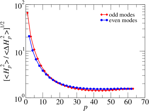
Figure 1: (Color online) The ratio $[\langle H_{p}^{2}\rangle/\langle\Delta H_{p}^{2}\rangle]^{1/2}$ for a dsDNA chain of length $N=63$.

V.1 Comparing ${\bf H}_{p}$ and $\Delta{\bf H}_{p}$ for dsDNA

Both ${\bf H}_{p}$ and $\Delta{\bf H}_{p}$ are fluctuating quantities, so a proper comparison between them would be to plot the ratio of $[\langle H_{p}^{2}\rangle/\langle\Delta H_{p}^{2}\rangle]^{1/2}$ as a function of $p$. In doing so we note that odd-$p$ modes are even under reversal of renumbering the beads from $n$ to $N-n$ and even-$p$ modes are odd under this reversal. Since the ground state is even under this reversal, it means that the odd-$p$ modes are excited more by thermal fluctuations. We therefore plot this ratio separately for the even and the odd modes in Fig. 1 for a dsDNA with $N=63$, i.e., a dsDNA chain 64 basepairs long. The plot shows the approximation scheme (45) in action — for low $p$-values, i.e., modes corresponding to large length-scales, the remainder $\Delta{\bf H}_{p}$ is only a fraction of ${\bf H}^{(0)}_{p}$. This opens up a systematic way of dealing with $\Delta{\bf H}_{p}$ that still couples the different (Rouse) modes, which we exploit in the next subsection.

V.2 Testing the vulnerability of the algorithm to enlarging $\Delta\tau$ for dsDNA

As already pointed in Sec. IV.1, with the approximations (50-53) we cannot limitlessly increase $\Delta\tau$. We now test numerically on dsDNA how far we can go on with increasing $\Delta\tau$ for $N=63,127,255$ and $511$. In other words, we obtain the values of $\Delta\tau_{\text{max}}$ for these values of $N$. The quantities we track, collectively denoted by $Q(t)$, in order to determine $\Delta\tau_{\text{max}}$ are the autocorrelation functions in time of (i) the end-to-end vector and (ii) the middle bond, and (iii) the mean-square displacement (msd) of the middle bead wrt the position of the centre-of-mass of the chain. Our test procedures are divided into two groups: the equilibrium values for these quantities, collectively denoted as $Q(0)$ and their dynamical behaviour. The test procedure is as follows.

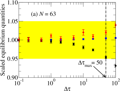
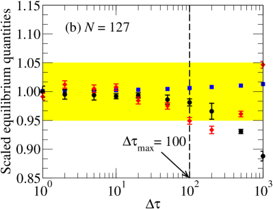
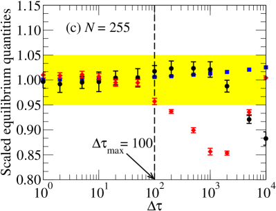
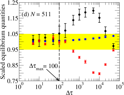
Figure 2: (Color online) Determination of $\Delta\tau_{\text{max}}$ from the equilibrium values $Q(0)$. The autocorrelation functions in time of the end-to-end vector are shown in black circles, the middle bond in blue squares, and the mean-square displacement (msd) of the middle bead wrt the position of the centre-of-mass of the chain in red diamonds. The data are rescaled by their MC values: (a) $N=63$, (b) $N=127$, (c) $N=255$ and (d) $N=511$. The error bars for the autocorrelation functions in time of the middle bond are not shown since they are smaller than the symbol size. The yellow band represents $5\%$ validity thresholds. See text for details.

In the first group, we determine the quantities (i-iii) for several values of $\Delta\tau$, namely (a) $N=63:\Delta\tau=$0.1, 0.2, 0.5, 1, 2, 5, 10, 20, 50 and 100, (b) $N=127:\Delta\tau=$1, 2, 5, 10, 20, 50, 100, 200, 500 and 1000, (c) $N=255:\Delta\tau=$1, 2, 5, 10, 20, 50, 100, 200, 500, 1000, 2000, 5000 and 10000, (d) $N=511:\Delta\tau=$ 5, 10, 20, 50, 100, 200, 500, 1000, 2000, 5000, 10000, 20000 and 50000. The data are averaged over 13 realisations of run length $\tau=8\times 10^{7}$ for $N=63$, $\tau=8\times 10^{8}$ million for $N=127$, $\tau=8\times 10^{9}$ for $N=255$ and $\tau=4\times 10^{10}$ for $N=511$ for each realisation. In the first group of tests we determine their equilibrium values as a function of $\Delta\tau$. As benchmarks of these equilibrium quantities we also perform Monte Carlo (MC) simulations, which are carried out again by using the mode representation, permitting one to take large MC steps in the slow modes and small steps in the fast modes. We accept the runs as valid if all measured observables deviate at most $5\%$ from their MC values, the other ones we reject as invalid, leading to a set of $\Delta\tau_{\text{max}}$ values for each $N$.

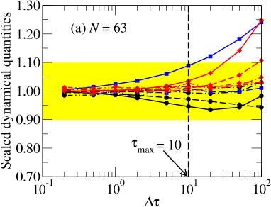
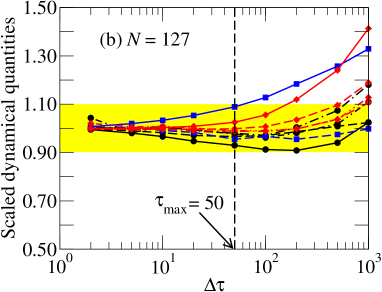
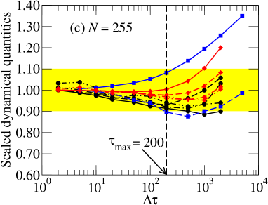
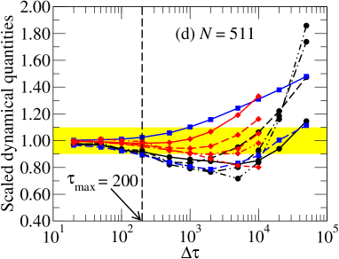
Figure 3: (Color online) Determination of $\Delta\tau_{\text{max}}$ from $Q(t)$. The autocorrelation functions in time of the end-to-end vector are shown in black circles, the middle bond in blue squares, and the mean-square displacement (msd) of the middle bead wrt the position of the centre-of-mass of the chain in red diamonds. The data are rescaled by $\tilde{Q}(\Delta\tau_{\text{min}})$. (a) $N=63$ ($\Delta\tau_{\text{min}}=0.1$): $\tau=100$ (solid line), 1000 (long-dashed), 10000 (dashed-dot-dashed), 100000 (dashed-dot-dot-dashed); (b) $N=127$ , ($\Delta\tau_{\text{min}}=1$): $\tau=1000$ (solid line), 10000 (long-dashed), 100000 (dashed-dot-dashed), 1000000 (dashed-dot-dot-dashed); (c) $N=255$ ($\Delta\tau_{\text{min}}=1$): $\tau=10000$ (solid line), 100000 (long-dashed), 1000000 (dashed-dot-dashed), 10000000 (dashed-dot-dot-dashed) and (d) $N=511$ ($\Delta\tau_{\text{min}}=5$): $\tau=100000$ (solid line), 1000000 (long-dashed), 10000000 (dashed-dot-dashed), 100000000 (dashed-dot-dot-dashed). The yellow band represents $10\%$ validity thresholds. See text for details.

The procedure is demonstrated in Fig. 2. We scale the equilibrium values by the corresponding MC ones, which means that the $y$-values of the rescaled equilibrium quantities should lie between 0.95 and 1.05, indicated by the yellow band representing our acceptance threshold. The highest $\Delta\tau$ values, for which all the equilibrium quantities — taking into consideration the error bars — fall within the yellow band gets us the $\Delta\tau_{\text{max}}$ values for each $N$ for the first group of test.

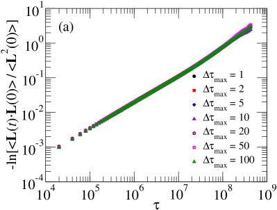
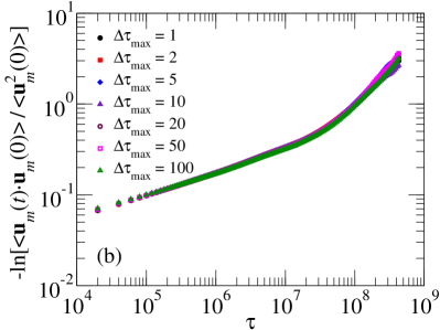
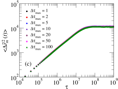
Figure 4: (Color online) The $Q(t)$ curves for $\Delta\tau=\Delta\tau_{\text{min}}$ to $\Delta\tau_{\text{max}}$ for $N=255$: the normalised autocorrelation function of the end-to-end vector ${\mathbf{L}}$ (a) and the middle bond vector ${\mathbf{u}}_{m}$ (b), and the means-square displacement $\langle\Delta\tilde{r}^{2}_{m}(t)\rangle$ of the middle bead measured wrt the centre-of-mass of the chain (c). The data for all values of $\Delta\tau$ coincide, as they should. The figure thus demonstrates the validity of our procedure.

In the second group of tests we use time-dependent quantities $Q(t)$. In this case MC simulations are of no help, so we treat the lowest value of $\Delta\tau$ for each $N$ as the benchmark. Let us describe the procedure for $N=63$, for which the lowest value of $\Delta\tau$ equals $\Delta\tau_{\text{min}}=0.1$. We choose a few fixed values of the time $\tau$, such as $\tau=100$, 1000, 10000 and 100000; first obtain the quantities $Q(\tau)$ and numerically differentiated quantity $dQ(\tau)/d\tau$ for all values of $\Delta\tau$, and thereafter the effective decay constant for $Q(\tau)$, i.e., ratio $\tilde{Q}(\tau)=\displaystyle{\frac{1}{Q(\tau)}\frac{dQ(\tau)}{d\tau}}$. [Clearly, for a given value of $\tau$, $\tilde{Q}(\tau)$ is also a function of $\Delta\tau$, i.e., $\tilde{Q}(\tau)\equiv\tilde{Q}(\tau,\Delta\tau)$.] We then demand that at these values of $\tau$ the ratio $\tilde{Q}(\Delta\tau)/\tilde{Q}(\Delta\tau_{\text{min}})$ does not deviate from unity by more than $10\%$. The $10\%$ is chosen by the following criterion: the statistical errors in the quantities $Q(t)$ are typically of order $2\%$, which accumulate to $\sim 4\%$ for $\tilde{Q}(t)$, to which we need to add our $5\%$ criterion as explained above, and further round their sum off to $10\%$. (The larger tolerance for the dynamical variables is a consequence of a lack of clean benchmark data, which was provided by MC simulations for equilibrium observables.) The result of this procedure is presented in Fig. 3 — note that this (numerical) procedure is prone to noise more than it has been for the first group that involved $Q(0)$, so we only carry out the procedure for which the procedure is not spoiled by noise in the data.

The results from the two figures 2-3 are summarised in Table 2. The final value of $\Delta\tau_{\text{max}}$ for any given value of $N$ is clearly the smaller one emerging from the two groups. Said differently, use of the final values of $\Delta\tau_{\text{max}}$ (as it appears in Table 2) in simulations means that the data for $Q(t)$ should not differ from each other by more than $5\%$ at any time. As an example of the validity of our procedure, we plot the $Q(t)$ curves for $N=255$ in Fig. 4 — for all $\Delta\tau$ values between $\Delta\tau_{\text{min}}$ and $\Delta\tau_{\text{max}}$ the curves are on top of each other as they should be.

$\quad N\quad$	$\quad\Delta\tau_{\text{max}}$ from equilibrium	$\quad\Delta\tau_{\text{max}}$ from dynamical	final $\Delta\tau_{\text{max}}\quad$
	quantities $Q(0)$	quantities $Q(t)$	min[columns 2 and 3]
63	50	10	10
127	100	50	50
255	100	200	100
511	100	200	100

Table 2: List of $\Delta\tau_{\text{max}}$ values for the values of $N$ studied in this paper for dsDNA.

VI Coarse-graining in our model

Up until now we have chosen the average spacing between the beads to coincide with the length of a dsDNA basepair $\approx 0.33$ nm. There is nothing special about this choice. In this section we explore the case when the average spacing between the beads is larger than the length of a dsDNA basepair, i.e., coarse-graining in our model, and its consequences.

While coarse-graining, we note that we have to consistently conform to the force extension curve for the dsDNA. The force extension relation proposed by Wang et al. wang has the form

$$\frac{Fl_{p}}{k_{B}T}=\frac{1}{4}\left[{1-\frac{\langle L\rangle}{L_{c}}+\frac{F}{K_{0}}}\right]^{-2}-\frac{1}{4}+\frac{\langle L\rangle}{L_{c}}-\frac{F}{K_{0}},$$ (54)

where $F$ is the applied force and $\langle L\rangle$ the average extension. The equation contains two empirical parameters: the persistence length $l_{p}$ and the force constant $K_{0}$. We convert them in dimensionless quantities as

$$r=\frac{l_{p}}{a},\quad\quad\quad y=\frac{l_{p}K_{0}}{k_{B}T},$$ (55)

where $a$ is the length of a basepair. The model parameters $T^{*}$ and $\nu$ are calculated by a fit to this force-extension curve as leeuwen

$$T^{*}=\frac{(2r^{2}+y)r}{y^{2}}\quad\quad\quad{\rm and}\quad\quad\quad\nu=\frac{r^{2}}{2r^{2}+y}.$$ (56)

We now make the choice for the discretization distance to be a multiple of the length of a basepair, and represent it by $ka$. With this choice, the parameter $l_{p}/a$ for the force extension curve changes from $r$ to $r_{k}=r/k$. The force constant $K_{0}$ and the persistence length $l_{p}$ must remain the same for the coarse-grained description of the chain, implying that $y$ remains the same as well. The new parameters $T^{*}_{k}$ and $\nu_{k}$ for our model then read

$$T^{*}_{k}=\frac{(2r^{2}+k^{2}y)r}{k^{3}y^{2}},\quad\quad\quad\nu_{k}=\frac{r^{2}}{2r^{2}+k^{2}y}.$$ (57)

Thus with increasing $k$ the model travels through a sequence of parameter points $(T^{*}_{k},\nu_{k})$ all leading to the same force-extension curve (54). As long as $k\ll r$ the loss of information due to coarse-graining will be small and the parameters $(T^{*}_{k},\nu_{k})$ will adequately describe the polymer at the chosen coarse-grained level. Moreover, while coarse-graining we must remember that the average inter-bead spacing should not exceed the persistence length, i.e., $k$ should stay well below $r$. In Table 3 below we give a set of parameters $(T^{*}_{k},\nu_{k})$ for a number of values of $k$.

$k$	$T^{*}_{k}$	$\nu_{k}$
$\quad 1\quad$	$\quad 0.034\quad$	$\quad 0.35\quad$
$\quad 2\quad$	$\quad 0.008\quad$	$\quad 0.1875\quad$
$\quad 5\quad$	$\quad 0.002192\quad$	$\quad 0.0437956\quad$
$\quad 10\quad$	$\quad 0.001024\quad$	$\quad 0.0117188\quad$
$\quad 12\quad$	$\quad 0.000847\quad$	$\quad 0.00819672\quad$
$\quad 15\quad$	$\quad 0.000673\quad$	$\quad 0.00527704\quad$
$\quad 20\quad$	$\quad 0.000503\quad$	$\quad 0.00298211\quad$

Table 3: Parameter values for dsDNA for our model under coarse-graining. With increasing $k$ the model travels through a sequence of parameter points $(T^{*}_{k},\nu_{k})$, all leading to the same force-extension curve (54). The case $k=1$ corresponds to the situation when the inter-bead spacing is the length of a basepair, $\approx 0.33$ nm.

VI.1 The $\nu\rightarrow 0$ limit and the inextensible WLC model

In Table 3 we observe that with increasing degree of coarse-graining the value of $\nu$ becomes progressively smaller. Since the condition $k<r$ provides an upper bound for $k$, the range of $k$ is rather small for the dsDNA to get really close to zero. (This is however not the case for f-actin, for which the table analogous to Table 3 can be found in Appendix A.) In the limit $\nu=0$, i.e., $\lambda\rightarrow\infty$ at fixed $\kappa$ — this is the same limit $k_{x}\rightarrow\infty$ for the extensible WLC, c.f. Sec. II.2 — our model physically approaches a discretised version of the inextensible WLC model. In this limit the chain gets stiffer to stretching but keeps the same persistence length. In this section we discuss how, in the case of $\nu\rightarrow 0$, the straightforward Euler method of integrating the bead positions leads to an algorithm similar to the one developed by Morse morse ; montesi .

For the limit $\nu\rightarrow 0$ at fixed $\kappa$ the time scaling $\tau=\lambda t/\xi$ that we have been using so far, is not useful. In this time scaling the coefficient of the stretching force is set to unity. But now we employ a time scaling where $\lambda$ is replaced by $\kappa$, such that the coefficient of the bending forces equals unity. The corresponding transformation, which we indicate with a bar over the new variables, reads

$$\bar{\tau}=\kappa t/\xi=\nu\tau,\quad\quad\bar{T}^{*}=T^{*}/\nu,\quad\quad\bar{\bf g}_{n}={\bf g}_{n}\nu,$$ (58)

The reduced Hamiltonian then obtains the form

$$\bar{\cal H}^{*}=\left[\frac{1}{2\nu}\sum^{N}_{n=1}(|{\bf u}_{n}|-1)^{2}-\sum^{N-1}_{n=1}{\bf u}_{n}\cdot{\bf u}_{n+1}\right].$$ (59)

In terms of these new variables the dynamic equations change to

$$\frac{d{\bf r}_{n}}{d\bar{\tau}}=-\frac{\partial\bar{\cal H}^{*}}{\partial{\bf r}_{n}}+\bar{\bf g}_{n}$$ (60)

with the correlation function

$$\langle\bar{g}^{\alpha}_{m}(\bar{\tau})\bar{g}^{\beta}_{n}(\bar{\tau}^{\prime})\rangle=2\,\bar{T}^{*}\delta^{\alpha,\beta}\delta_{m,n}\delta(\bar{\tau}-\bar{\tau}^{\prime}).$$ (61)

In order to implement the limit $\nu\rightarrow 0$, we symbolically write the equations of motion for the beads as

$$\frac{d{\bf r}_{n}}{d\bar{\tau}}={\bf f}_{n}=-\frac{\partial\bar{\cal H}^{*}}{\partial{\bf r}_{n}}+\bar{\bf g}_{n}=-\frac{\partial\bar{\cal H}^{*}}{\partial{\bf u}_{n}}+\frac{\partial\bar{\cal H}^{*}}{\partial{\bf u}_{n+1}}+\bar{\bf g}_{n}.$$ (62)

The differentiation in Eq. (62) is straightforward, with exception of the first term in Eq. (59) which we write as

$$\frac{\partial}{\partial{\bf u}_{n}}\frac{1}{2\nu}\left(\sum^{N}_{m=1}(|{\bf u}_{m}|-1)^{2}\right)\equiv f^{\nu}_{n}\,{\bf u}_{n}.$$ (63)

The quantity $f^{\nu}_{n}$ may be considered as a “tension” that keeps the length of the $n$-th bond close to unity. It obtains a finite limit for $\nu\rightarrow 0$. Once we have an expression for the $f^{\nu}_{n}$, the dynamical equations follow. We determine the value of $f^{\nu}_{n}$ by the requirement that it keeps the evolution of the chain configuration on the constrained subspace $u_{n}=1$; i.e., $f^{\nu}_{n}$ play the same role as the Lagrange multipliers that preserve the contour length of the chain at all times in the discretised version of the WLC morse .

Since the $f^{\nu}_{n}$ are still undetermined we write the equations of motion (63) as

$$\frac{d{\bf r}_{n}}{d\bar{\tau}}=-f^{\nu}_{n}\,{\bf u}_{n}+f^{\nu}_{n+1}{\bf u}_{n+1}+{\bf f}^{r}_{n},$$ (64)

where ${\bf f}^{r}_{n}$ contains the regular terms of the forces. Let us then consider a finite increment $\Delta\tau$ in time. In this time interval the bond vector ${\bf u}_{n}$ changes by the amount

$$\Delta{\bf u}_{n}=\left(f^{\nu}_{n-1}{\bf u}_{n-1}-2f^{\nu}_{n}\,{\bf u}_{n}+f^{\nu}_{n+1}{\bf u}_{n+1}+{\bf f}^{r}_{n}-{\bf f}^{r}_{n-1}\right)\Delta\tau,$$ (65)

leading to the tentative new value of the bond vector as

$${\bf u}^{\prime}_{n}={\bf u}_{n}+\Delta{\bf u}_{n}.$$ (66)

Now requiring that $u^{\prime}_{n}=u_{n}=1$ leads to the equations

$$2{\bf u}_{n}\cdot\Delta{\bf u}_{n}+\Delta{\bf u}_{n}\cdot\Delta{\bf u}_{n}=0\quad\quad{\rm or}\quad\quad({\bf u}_{n}+{\bf u}^{\prime}_{n})\cdot\Delta{\bf u}_{n}=0.$$ (67)

As we do not a priori know ${\bf u}^{\prime}_{n}$, we first take as zeroth order approximation ${\bf u}^{\prime}_{n}={\bf u}_{n}$ and solve for $\Delta{\bf u}_{n}$ in the second equation (67). Then we compute the first approximation to ${\bf u}^{\prime}_{n}$ with equation (66) and iterate the cycle till it converges, which is typically reached in two or three steps.

The structure of the second equation (67) is

$$\begin{array}[]{rcl}\left(\begin{array}[]{rcclcc}-2&b_{1}&0&0&\cdots&0\\[5.69054pt] b_{1}&-2&b_{2}&0&\cdots&0\\[5.69054pt] 0&b_{2}&-2&b_{3}&\cdots&0\\[5.69054pt] \cdots&\cdots&\cdots&\cdots&\cdots&\cdots\\[5.69054pt] 0&\cdots&0&b_{N-2}&-2&b_{N-1}\\[5.69054pt] 0&\cdots&0&0&b_{N-1}&-2\\[5.69054pt] \end{array}\right)\left(\begin{array}[]{c}f^{\nu}_{1}\\[5.69054pt] f^{\nu}_{2}\\[5.69054pt] f^{\nu}_{3}\\[5.69054pt] \cdots\\[5.69054pt] f^{\nu}_{N-1}\\[5.69054pt] f^{\nu}_{N}\\[5.69054pt] \end{array}\right)&=&\left(\begin{array}[]{c}d_{1}\\[5.69054pt] d_{2}\\[5.69054pt] d_{3}\\[5.69054pt] \cdots\\[5.69054pt] d_{N-1}\\[5.69054pt] d_{N}\\[5.69054pt] \end{array}\right),\end{array}$$ (68)

with

$$b_{n}={\bf u}_{n}\cdot{\bf u}_{n+1},\quad\quad\quad{\rm and}\quad\quad\quad d_{n}=({\bf u}_{n}+{\bf u}^{\prime}_{n})\cdot({\bf f}^{r}_{n-1}-{\bf f}^{r}_{n}).$$ (69)

As the matrix in Eq. (68) is tridiagonal, the solution $f^{\nu}_{n}$ is obtained by an ${\cal O}(N)$ operation. With the converged $\Delta{\bf u}_{n}$ we update the bond vectors (which is equivalent to updating the positions, since the centre-of-mass of the chain is not affected by the motion).

This implementation of the inextensible WLC is an alternative for the standard procedure of implementing the constraints morse using Lagrange multipliers that preserve the contour lengths of the chain at all times. Not only that the parameters $f^{\nu}_{n}$ play the same role as the Lagrange multipliers, but also the equations for the $f^{\nu}_{n}$ are similar to the ones for the Lagrange parameters, involving the same matrix as in Eq. (68). The difference is in the right hand side of Eq. (69) and the definition of the remaining forces ${\bf f}^{r}_{n}$ which involve in the standard procedure additional metric pseudo-forces. Moreover, if we systematically evaluate the forces at the midpoint

$${\bf u}^{m}_{n}=({\bf u}_{n}+{\bf u}^{\prime}_{n})/|{\bf u}_{n}+{\bf u}^{\prime}_{n}|,$$ (70)

then this scheme is symmetric in time between forward and backward motion, which implies that detailed balance is obeyed to third order in the displacements.

VII $\Delta\tau_{\text{max}}$ values for double-stranded DNA

VII.1 Time step for the inextensible WLC

For a fair comparison between the maximum allowable time-step $\Delta\bar{\tau}_{\text{max}}$ between our model and the inextensible WLC we have simulated our model at fixed values of $l_{p}/a$ (or $\kappa$) for a series of decreasing values of the parameters $\nu$. In order to stay close to dsDNA we have taken the value of $l_{p}/a$ of dsDNA. For the chain length $N=63$ beads we use the (default) Euler scheme.

Recall from Sec. III.1 that for $\nu=0.35$ nm the safe limit for the Euler scheme for the bead position updates is $\Delta\tau=0.1$, and the code becomes even unstable at $\Delta\tau\approx 0.3$. Such instabilities also occur for other values of $\nu$, and with progressively smaller values of $\nu$ we found the stability limit to behave as $\Delta\bar{\tau}\simeq 0.6\nu$ — the $\nu$ dependence comes from the factor $1/\nu$ in the harmonic confining potential [the first term in the Hamiltonian (59)]. So if we were to study the maximum allowable time step from a series for decreasing $\nu$, we would end up with time step zero for in the limit $\nu\rightarrow 0$.

The limit procedure as developed in Sec. VI.1 instead leads to a finite allowable timestep, which thus is the largest that can be used for small values of $\nu$ or in the inextensible limit. We find that a time step $\Delta\bar{\tau}=0.00005$ gets the equilibrium average end-to-end distance and the average of the squared displacement of the middle monomer within 5% of the theoretically calculated values. Translating this value to the scaling used by Obermayer and Frey ober (who implemented Morse’s algorithm morse ; montesi , and used the coefficient of the fluctuations of the random forces to be equal to 2 as opposed to $2\bar{T}^{*}$ as we have used) we get a value $5\times 10^{-6}$ for the time-step, which is of the same order as used by them.

From this analysis one sees that using the forward Euler scheme, modelling dsDNA as an (extensible) bead-spring model (that leads to $\nu=0.35$) we get to $\Delta\tau_{\text{max}}=0.1$, which translates to $\Delta\bar{\tau}_{\text{max}}\approx 0.035$, while the same scheme for inextensible WLC leads to $\Delta\bar{\tau}_{\text{max}}=0.00005$. I.e., just by allowing the chain to be naturally extensible into account we gain a factor $\sim 10^{3}$ in the time-step.

VII.2 Translating $\Delta\tau_{\text{max}}$ to real times

We now translate $\Delta\tau_{\text{max}}$ to real times using the experimental parameters characteristic for dsDNA.

To this end we note that in Langevin dynamics there are no hydrodynamic interactions among the beads, leading to the centre-of-mass diffusion of a single chain $D=k_{B}T/(N\xi)$. In experiments hydrodynamic interactions are always present, however, they only become important when the chain is long enough to exhibit self-avoiding walk statistics. Thus, as long as the chains are substantially smaller than the persistence length, they behave essentially as straight rods, for which hydrodynamic interactions among beads are not important. In other words, for chains substantially smaller than the persistence length we can meaningfully compare the centre-of-mass diffusion coefficient resulting from our model and experiments. This comparison then yields us the correspondence of $\Delta\tau_{\text{max}}$ to real times.

The diffusion coefficient of small dsDNA segments has been studied using various techniques, such as capillary electrophoresis stellwagena ; stellwagenb , dynamic light scattering dls , NMR nmr , and fluorescent recovery after photobleaching frap . Of these, the first three converge on the value $D\approx 1.07\times 10^{8}$ nm²/s for a 20 bp dsDNA in water at room temperature ($23^{\circ}$ C), while the last one reports $5.3\times 10^{7}$ nm²/s for dsDNA segment of length 21 bp. We decide to stick to the values reported by the first three because of the consistency among different experimental methods, and upon equating $D=k_{B}T/(N\xi)$ to $\approx 1.07\times 10^{8}$ nm${}^{2}/$s for $N=20$, with $k_{B}T=4.089$ pN nm at $23^{\circ}$ C, we obtain

$$\xi=1.91\times 10^{-12}\mbox{\,kg/s}.$$ (71)

Further, writing the relation $t=\xi\tau/\lambda$ [see Sec. II, and the paragraph above Eq. (16)], in terms of the parameters $T^{*}$ and $\nu$, the conversion between the real time $t$ and the dimensionless time $\tau$ is obtained as

$$t=\frac{T^{*}}{b^{2}}\,\frac{a^{2}\xi}{k_{B}T}\,\tau=\nu\,\frac{a}{l_{p}}\,\frac{a^{2}\xi}{k_{B}T}\,\tau.$$ (72)

The combination $a^{2}\xi/(k_{B}T)$ is with $a=0.33$ nm and the value of $\xi$ from Eq. (71) equal to

$$\frac{a^{2}\xi}{k_{B}T}=52.0\mbox{\, ps}.$$ (73)

Inserting the dsDNA values $l_{p}/a=114$ and $\nu=0.35$ one gets

$$t\equiv c\tau,\quad\quad{\rm with}\quad\quad c=0.16\mbox{\, ps}.$$ (74)

i.e. one unit of dimensionless time corresponds to $0.16$ ps of real time. For the sake of completeness, the corresponding conversion factor between $t$ and $\bar{\tau}$ is given by

$$t\equiv\bar{c}\bar{\tau},\quad\quad{\rm with}\quad\quad\bar{c}=0.45\mbox{\, ps}.$$ (75)

chain length (bp)	$\quad\Delta\tau_{\text{max}}\quad$	$\quad\Delta t_{\text{max}}$ (ps)	$\quad t_{\text{max}}$ (ms)
64	10	1.59	0.23
128	50	7.96	0.56
256	100	15.9	0.56
512	100	15.9	0.25

Table 4: Time forward integration steps $\Delta t_{\text{max}}$ in real times for various chain lengths. Also noted in the last column the amount of real time $t_{\text{max}}$ our model can simulate on a standard linux desktop computer in one hour.

With the above information we can now translate $\Delta\tau_{\text{max}}$, the maximum time step, to real times $\Delta t_{\text{max}}$ in Table 4. Also noted in the last column of Table 4 is the amount of real time $t_{\text{max}}$ our model can simulate in an hour on a standard linux desktop computer.

For completeness we mention the conversion of $\bar{\tau}$ to real times, which is useful for small $\nu$ as occurring in the coarse-grained representation of the polymer. This conversion reads in analogy with (72)

$$t=\frac{\bar{T}^{*}}{b^{2}}\,\frac{a^{2}\xi}{k_{B}T}\,\bar{\tau}=\frac{a}{l_{p}}\,\frac{a^{2}\xi}{k_{B}T}\,\bar{\tau}.$$ (76)

With $\Delta\bar{\tau}_{\text{max}}\approx 0.00005$ we find $\Delta t_{\text{max}}\approx 0.02$ fs, for dsDNA in the inextensible WLC limit, which is about 5-6 orders of magnitude smaller than those listed in the second column of Table 4.

$k$	$c_{k}=t/\tau$ in ps
$\quad 1\quad$	$\quad 1.54\quad$
$\quad 2\quad$	$\quad 13.09\quad$
$\quad 5\quad$	$\quad 119.434\quad$
$\quad 10\quad$	$\quad 511.327\quad$
$\quad 12\quad$	$\quad 741.622\quad$
$\quad 15\quad$	$\quad 1165.66\quad$
$\quad 20\quad$	$\quad 2081.9\quad$

Table 5: The ratio between the real time $t$ and the scaled time $\tau$ under coarse-graining, with coarse-graining parameter $k$. The corresponding values of $T^{*}_{k}$ and $\nu_{k}$ can be found in Table 3.

We also note that coarse-graining increases the factor between real and scaled time substantially, as can be seen from Table 5. For the dimerized dsDNA chain we show in Fig. 5 the time evolution of the MSD of the end-to-end vector for a chain of 256 base pairs and that of 128 dimerized base pairs. Both have the same force-extension curves and the latter is simulated with the parameters $T^{*}_{2}=0.008$ and $\nu_{2}=0.1875$. The figure shows that the correspondence between the two is excellent. In general, the net gain in real time upon coarse-graining remains modest: although the value of $c_{k}$ increases with $k$ as listed in Table 5, it also leads to smaller $\nu_{k}$, further leading to smaller allowable time steps, as discussed in Sec. VII.1. The eventual largest time-step under coarse-graining for dsDNA, in real time, is still larger than the allowable time step for the $\nu=0$ case for inextensible WLC; i.e., even with a small $\nu_{k}$ it remains efficient to use the model rather than the limit $\nu=0$ procedure. A further advantage of coarse-graining is that longer polymers can be simulated in the time associated with the smaller number of beads, but that is true for any model.

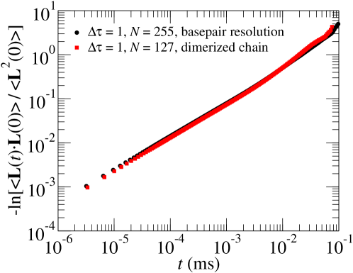
Figure 5: (Color online) The end-to-end vector data for a chain of 256 base pairs and that of the corresponding chain of 128 dimerized basepairs.

VIII Conclusion

Using a recently developed bead-spring model, in the absence of hydrodynamic interactions among the beads, in this paper we have developed an efficient algorithm to simulate the dynamics of dsDNA as a semiflexible polymer. Polymer dynamics in the model is described by the Langevin equation. We consider dsDNA at persistence length $l_{p}\approx 37.7$ nm that corresponds to $114$ beads in the model. The model can be mapped one-on-one to the extensible WLC. We show that, within an accuracy tolerance level of $5\%$ of several key observables, the model allows for large single Langevin time steps; as summarised in Table 4.

The key to such large time steps is to use the polymer’s fluctuation modes as opposed to the individual beads for simulating the dynamics. The conventional simulation approach would be to integrate the corresponding Langevin equations of motion in time, with a simple integration scheme such as the Euler method. This is however, not an efficient method, as one can get to $\Delta t_{\text{max}}$ to $\approx 0.16$ ps; at $\Delta t_{\text{max}}\approx 0.48$ ps the integration algorithm even becomes unstable. Instead, we use the polymer’s fluctuation modes to integrate the dynamical equations forward in time. Although any choice of orthogonal basis functions can be used to describe the polymer’s fluctuation modes, we found that the choice of the Rouse modes provides the most stable and robust results. Use of the Rouse modes allows us to take 2 to 3 orders of magnitude larger time steps for integrating the Langevin equations forward in time, as evidenced in Table 4.

We remark that the numbers in the table are only indicative for the order of magnitude of the allowable time step for various reasons. First of all, the choice 5% for the equilibrium quantities (consistently, 10% for the dynamical quantities) is arbitrary. Secondly, the percentage error in the physical observables depends on the quantity chosen. We find that in most cases the msd of the middle monomer decides the size of $\Delta t_{\text{max}}$. The end-to-end vector also plays that role in a few cases, while the middle bond is not at all critical. For the accuracy percentage (of course) it also matters whether one takes e.g. the square of the end-to-end vector (as we did) or the vector itself (the latter choice halves the error). Finally, the maximum allowable time step depends also on the parameters $T^{*}$ and $\nu$. We found that the dependence on $T^{*}$ is rather weak but the sensitivity to the value of $\nu$ is much stronger. Nevertheless, despite these reservations, the gain of 2 to 3 orders of magnitude by changing the integration variables from bead positions to Rouse modes stands firm. Importantly, a similar speed-up can also be achieved for the extensible WLC, since our model can be mapped one-on-one to it.

Like almost any other model, ours allows for coarse-graining. As the model is restricted to conform to the force-extension curve, the two parameters of the model $T^{*}$ and $\nu$ travels through a sequence of points, all leading to the same force-extension curve. We have shown that $\nu$ becomes progressively smaller under increasing degree of coarse-graining. Although not really applicable to the case for dsDNA (but certainly for f-actin), $\nu$ can be made to become so small that physically our model approaches the limit of inextensible WLC. We have shown that in the limit of $\nu\rightarrow 0$ the dynamical equations of the beads approach a form similar to the ones developed by Morse morse ; montesi for simulating the inextensible WLC. Using these equations we have simulated a dsDNA chain of length $N=63$ in the inextensible limit using the bead positions as dynamical variables (with the default Euler updating scheme). By means of doing so,we have demonstrated that just by changing the model from inextensible to extensible bead-spring we gain $\approx 3$ orders of magnitude in the size of the time-step. Combining this speed-up with the ones achieved by using the Rouse modes as integration variables as opposed to the bead positions, we have achieved 5-6 orders of magnitude speed-up in the size of the time-step in comparison to the inextensible WLC.

Further, we note that Langevin dynamics simulations are widely used for the simulation of biopolymers, but most publications do not present a clear translation of the simulation time in real time (picoseconds or nanoseconds) and the experimental observation used to make this translation; and certainly do not explore the maximal time step which does not cause significant systematic errors. We found reports of time steps of 12.9 ps timestep1 , 5 ps timestep2 and 3.8 ps timestep3 , in simulations in which a bead represents 4, 9 and 37 basepairs respectively; A back-of-the-envelop estimate then yields that by-and-large, these time steps are below the maximal time step estimated by us for an integration scheme in real-space coordinates.

Finally, while our model is not well-suited for hard-core interactions, it does allow for adding other forces to the monomers. In order to showcase this, we have simulated dsDNA segments in a shear flow, where the viscous drag force due to the shear flow makes the chain tumble in space. The equations of motion Eq. (14) then become

$$\frac{d{\bf r}_{n}(t)}{dt}=-\frac{1}{\xi}\frac{\partial{\cal H}}{\partial{\bf r}_{n}}+\dot{\gamma}\,y_{n}\hat{\bf x}+{\bf g}_{n}(t),$$ (77)

where $\dot{\gamma}$ is the shear rate. These equations are easily transformed into mode equations. In the Supplementary Information we present a movie of a tumbling dsDNA chain of 255 base pairs; the chain tumbles in water with a velocity field ${\bf v}({\bf r})=\dot{\gamma}y\hat{x}$, with shear rate $\dot{\gamma}\approx 1.54\times 10^{8}$ s^-1 (which corresponds to Weissenberg number $\mbox{Wi}\approx 5.55\times 10^{3}$, calculated from the moment of inertia of a straight rod of the same length as the dsDNA segment leeuwen ; leeuwen1 ). In the movie the centre-of-mass of the chain always remains at the origin of the co-ordinate system. The data for the movie are generated with $\Delta t=\Delta t_{\text{max}}=16$ ps, and took about three minutes to generate on a linux desktop; it contains 3,000 snapshots, with consecutive snapshots being 8 ns apart. A detailed study of the tumbling motion of the dsDNA in a shear flow is however not the focus of this paper; it will be taken up in an upcoming one.

Appendix A Coarse-graining f-actin

The persistence length of f-actin is orders of magnitude longer than that of dsDNA. Liu and Pollack liu report values $l_{p}=8.75\,\mu$m for f-actin, while the length of actin monomer is 5.5 nm stef . Also the force constant $K_{0}$ is orders larger than the dsDNA value. Liu and Pollack find for $K_{0}=35.5$ nN. This leads to the dimensionless parameters

$$r=l_{p}/a=1591\quad\mbox{and}\quad y=7.65\times 10^{7}$$ (78)

for f-actin. In order to determine $\xi$, we use the information that the time taken for an actin filament with a contour length $L=10$ microns (corresponding to $N=L/a=1818$ beads) and a diameter of 5 nm in a solution with a viscosity of 0.1 Pa s (water) at a temperature of $20^{\circ}$C has to diffuse its own length is $t^{*}=1.5\times 10^{4}$ s. This leads us to the equation

$$t^{*}=L^{2}/(6D)=\xi L^{3}/(6ak_{B}T);\quad\mbox{i.e.,}\quad\xi=5.5\times 10^{-11}\,\,\mbox{kg/s},$$ (79)

where $D$ denotes the diffusion coefficient of the f-actin filament, further yielding

$$\frac{a^{2}\xi}{k_{B}T}\approx 0.4\,\,\mu\mbox{s}.$$ (80)

With these values we can now calculate with the expressions (56) the values of the effective $\bar{T}^{*}_{k}$ and $\nu_{k}$ for f-actin, which are shown in Table 6.

$k$	$\bar{T}^{*}_{k}$	$\nu_{k}$	$\bar{c}_{k}$ (in $\mu$s)
1	0.000713	0.030603	0.00025
2	0.001298	0.008019	0.00402
5	0.003159	0.001301	0.15713
10	0.006294	0.000326	2.51414
20	0.012575	8.14832 $\times 10^{-5}$	40.2263
50	0.031428	1.30391 $\times 10^{-5}$	1571.34

Table 6: Coarse-grained parameters for f-actin.

The variation in $\bar{T}^{*}_{k}$ with $k$ does not have significant consequences since $\bar{T}^{*}_{k}$ enters the dynamical equations only in the form of $\sqrt{\bar{T}^{*}_{k}}$. The decrease of $\nu_{k}$ with increasing $k$, on the other hand, has much more severe consequences on the dynamics, as it makes the chain effectively more inextensible. In contrast to dsDNA one already runs into — even for fairly mild coarse-graining — quite small values of $\nu_{k}$. E.g., for $k=50$, which would mean about 75 beads per persistence length, the value of $\nu_{k}$ is so small that for all practical purposes our model behaves (except of course the force-extension curve) as the inextensible WLC, and our maximum time-step then would then be $\Delta\bar{\tau}_{\text{max}}\approx 0.00005$.

Even more interesting is the ratio between the real time and the scaled time involving the $k$-dependent parameters [c.f. Eq. (76)]:

$$t=\bar{c}_{k}\bar{\tau}=k^{4}\frac{a}{l_{p}}\frac{a^{2}\xi}{k_{B}T}\bar{\tau}.$$ (81)

E.g., even with a small maximal allowable timestep $\Delta\bar{\tau}_{\text{max}}=0.00005$ the large value of $\bar{c}_{k}$ for $k=50$ leads to

$$\Delta t_{\text{max}}=0.00005\times 1571.34\times 0.4\,\mu{\rm s}=0.03\,\mu{\rm s}.$$ (82)

This is orders of magnitude larger than the order of picosecond estimates for $\Delta t_{\text{max}}$ for dsDNA.

References

- (1) C. Bustamante, J. F. Marko, E. D. Siggia and S. Smith, Science 265, 1599 (1994); J. F. Marko and E. D. Siggia, Macromolecules 28, 8759 (1995).
- (2) M. D. Wang, H. Yin, R. Landick, J. Gelles and S. M. Block, Biophys. J. 72 1335 (1997).
- (3) A. Ott et al., Phys. Rev. E 48, 1642 (1993).
- (4) F. Gittes, B. Mickey, J. Nettleton and J. Howard, J. Cell Biol. 120, 923 (1993).
- (5) G. T. Barkema and J. M. J. van Leeuwen, J. Stat. Mech. P12019 (2012).
- (6) G. T. Barkema, D. Panja and J. M. J. van Leeuwen, J. Stat. Mech. P11008 (2014).
- (7) B. Obermayer and E. Frey, Phys.Rev. E 80, 040801(R) (2009).
- (8) O. Kratky and G. Porod, Recl. Trav. Chim. Pays-Bas. 68, 1106 (1949).
- (9) J. J. Hermans and R. Ullman, Physica 18, 951 (1952).
- (10) H. Daniels, Proc. R. Soc. Edinburgh, Sect. A: Math. Phys. Sci. 63, 290 (1952).
- (11) N. Saito, K. Takahashi and Y. Yunoki, J. Phys. Soc. Jpn. 22, 219 (1967).
- (12) H. Yamakawa, Pure Appl. Chem. 46, 135 (1976).
- (13) C. Bouchiat et al., Biophys. J. 76, 409 (1999).
- (14) J. Wilhelm and E. Frey, Phys. Rev. Lett. 77, 2581 (1996).
- (15) J. Samuel and S. Sinha, Phys. Rev. E 66, 050801 (2002).
- (16) A. Dhar and D. Chaudhuri, Phys. Rev. Lett. 89, 065502 (2002).
- (17) P. Gutjahr, R. Lipowsky and J. Kierfeld, Europhys. Lett., 76, 994 (2006).
- (18) B. Obermayer, O. Hallatschek, E. Frey and K. Kroy, Eur. Phys. J. E 23, 375 (2007).
- (19) R.E. Goldstein, S.A. Langer, Phys. Rev. Lett. 75, 1094 (1995).
- (20) N.-K. Lee, D. Thirumalai, Biophys. J. 86, 2641 (2004).
- (21) Y. Bohbot-Raviv, W. Z. Zhao, M. Feingold, C. H. Wiggins, R. Granek, Phys. Rev. Lett. 92, 098101 (2004).
- (22) T. B. Liverpool, Phys. Rev. E 72, 021805 (2005).
- (23) J. T. Bullerjahn, S. Sturm, L. Wolff and K. Kroy, Europhys. Lett. 96, 48005 (2011).
- (24) D. C. Morse, Adv. Chem. Phys. 128, 65 (2004).
- (25) A. Montesi, D. C. Morse and M. Pasquali, J. Chem. Phys. 122, 084903 (2005).
- (26) L. Harnau, R. G. Winkler and P. Reineker, J. Chem. Phys. 104, 6355 (1996).
- (27) R. G. Winkler, J. Chem. Phys. 118, 2919 (2003).
- (28) P. S. Lang, B. Obermayer and E. Frey, Phys. Rev. E 89, 022606 (2014).
- (29) P. E. Rouse, J. Chem. Phys. 21, 1272 (1953).
- (30) C. Forrey and M. Muthukumar, Biophys. J. 91, 25 (2006).
- (31) S. A. Allison, R. Austin and M. Hogan, J. Chem. Phys. 90, 3843 (1989).
- (32) G. Chirico and J. Langowski, Biopolymers 34, 415 (1994).
- (33) N. C. Stellwagen, S. Magnusdóttir, C. Gelfi and P. G., Righetti, J. Mol. Biol. 305, 1025 (2001).
- (34) E. Stellwagen and N. C. Stellwagen, Electrophoresis 23, 2794 (2002).
- (35) W. Eimer and R. Pecora, J. Chem. Phys. 94, 2324 (1991).
- (36) G. F. Bonifacio, T. Brown, G. L. Conn and A. N. Lane, Biophys. J. 73, 1532 (1997).
- (37) G. L. Lukacs, P. Haggie, O. Seksek, D. Lechardeur, N. Freedman and A. S. Verkman, J. Biol. Chem. 275, 1625 (2000).
- (38) X. Liu and G.H. Pollack, Biophys. J. 83, 2705 (2002).
- (39) W. Steffen, D. Smith, R. Simmons and J. Sleep, Proc. Natl. Acad. Sci. (USA) 98, 14949 (2001).