Nonlinear predictive latent process models for integrating spatio-temporal exposure data from multiple sources

Abstract

Spatio-temporal prediction of levels of an environmental exposure is an important problem in environmental epidemiology. Our work is motivated by multiple studies on the spatio-temporal distribution of mobile source, or traffic related, particles in the greater Boston area. When multiple sources of exposure information are available, a joint model that pools information across sources maximizes data coverage over both space and time, thereby reducing the prediction error.

We consider a Bayesian hierarchical framework in which a joint model consists of a set of submodels, one for each data source, and a model for the latent process that serves to relate the submodels to one another. If a submodel depends on the latent process nonlinearly, inference using standard MCMC techniques can be computationally prohibitive. The implications are particularly severe when the data for each submodel are aggregated at different temporal scales.

To make such problems tractable, we linearize the nonlinear components with respect to the latent process and induce sparsity in the covariance matrix of the latent process using compactly supported covariance functions. We propose an efficient MCMC scheme that takes advantage of these approximations. We use our model to address a temporal change of support problem whereby interest focuses on pooling daily and multiday black carbon readings in order to maximize the spatial coverage of the study region.

FLA

, , and T1Supported by Grants from the National Institute of Environmental Health Sciences (ES07142, ES000002, ES012044, ES016454, ES009825), the National Cancer Institute (CA134294), and the U.S. Environmental Protection Agency (EPA) Grant R-832416. T2Supported by the postdoctoral training Grant CA090301 from the National Cancer Institute.

1 Introduction and background

An important scientific goal in environmental health research is the identification of sources of air pollution responsible for the well-documented health effects of air pollution. A pollution source of great interest is motor vehicle (i.e., traffic) emissions. Because traffic pollution is inherently higher near busy roads and major highways and falls off to background levels relatively quickly in space, concentrations of traffic-related pollutants exhibit large amounts of spatial heterogeneity within an urban area. Therefore, epidemiologic studies of the health effects of traffic pollution that use a centrally sited ambient monitor suffer from large amounts of exposure measurement error [Zeger et al. (2000)]. However, because it is not always feasible to obtain exposure recordings at each study subject’s residence at a given time (a special case of spatio-temporal misalignment), it is now common practice in air pollution epidemiology for researchers to collect data from monitoring networks on the intra-urban spatio-temporal variability in traffic pollution levels. These data are used to make predictions of the exposure process, which are then used as a surrogate for true exposures in health effects models [Adar et al. (2010); Berhane et al. (2004); Wannemuehler et al. (2009)]. Note that this creates a measurement error problem [Gryparis et al. (2009)].

In this article we consider statistical models for prediction of spatio-temporal concentrations of black carbon (BC), thought to be a surrogate for traffic-related air particle levels [Janssen et al. (2011)], in the greater Boston-area. One complicating factor in the development of such models in our Boston-area analysis, however, is that the logistical and financial demands of maintaining a dedicated monitoring network are prohibitive. Accordingly, rather than set up a single network with a standardized monitoring protocol, our collaborators have augmented existing ambient monitoring data with targeted residence-specific indoor pollution monitoring aimed at increasing both the spatial and temporal coverage of the study region and period, respectively. Early work by our group [Gryparis et al. (2007)] focused on latent variable models for the integration of spatio-temporal data from multiple sources when all data were measured at the same temporal (in this case, daily) scale. The resulting number of monitors producing daily BC data was modest (under 90), limiting our ability to fully explore the spatio-temporal structure in the data. Specifically, such data sparsity motivated us to fit relatively simple spatial models separately for warm and cold seasons, as opposed to fitting more complex and likely more realistic spatio-temporal correlation structures across the entire study period.

Since this initial work, data at additional spatial locations have been collected. In this work, we consider data from 93 additional indoor monitors and explore how incorporation of these data improves our ability to explore the spatio-temporal patterns in the resulting monitoring data and ultimately the predictive performance of the resulting exposure models. One factor complicating the integration of these new data is the fact that this more recent monitoring campaign yielded concentration data at temporal scales different than the original BC data. Whereas the original data were collected on a daily time scale, the more recent monitoring campaign yielded multiday integrated readings. Therefore, our scientific interest focuses on the integration of data from these disparate sources into a unified exposure prediction framework, while rigorously accounting for changes in temporal support and the fact that different monitors operate irregularly in time. Given a modeling strategy that satisfies these goals, we assess the improvement in predictive performance of the models that incorporate all the data versus simpler models that only use the original daily data. While there has been a wide body of statistical work on spatio-temporal modeling of air pollution, most of these efforts have focused on data without substantial temporal misalignment and with a single type of pollution measurement. Although there is a considerable literature on the change of spatial and spatio-temporal support [Gelfand, Zhu and Carlin (2001)] and the use of aggregated data in spatial statistics [Gotway and Young (2002, 2007); Fuentes and Raftery (2005)], these proposed methods largely rely on the linear change-of-support and data assimilation. For example, Calder (2007, 2008) develops dynamic process convolution models—effectively, multivariate time series models—for multivariate spatio-temporal air quality data that allow one to solve the linear change-of-support problem. We are not aware of references that focus on the nonlinear change of temporal support in spatio-temporal statistics.

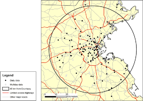
Figure 1: Spatial coverage of monitors. The HSPH (Countway) monitor is at the center of the circle in Downtown Boston.

We now outline the structure of the available BC data in more detail. The three data types that we use in our model and describe below are (i) daily average outdoor BC concentrations (abbreviated as BCO), (ii) daily average indoor BC concentrations (BCI) and (iii) multiday aggregated indoor BC concentrations (BCA), in $\mu g/m^{3}$. Figure 1 and Figure 4 of the online supplements [Bliznyuk et al. (2014)] display the spatial and temporal coverage of the study region and periods, distinguishing the different data types.

Daily outdoor data (BCO)

A sizeable fraction of the BCO readings that we use come from Gryparis et al. (2007). These data, generated from two different exposure assessment studies, were collected by outdoor monitors at 48 spatial locations in Boston and its suburbs over the period from mid October 1999 to the end of September 2004. The length of time each monitor operated ranged from 2 weeks to hundreds of days. These monitoring efforts resulted in 4219 daily BC readings. Our analyses supplement these data with additional daily BC data collected as part of a recent NIH Program Project Grant (PPG), which added 2696 daily readings from 52 distinct sites taken between mid March 2006, and early November 2008. The observations from the two studies do not occur at the same spatial locations, thus, we have 100 distinct sites, with over 6900 daily BCO readings.

Daily indoor data (BCI)

These data consist of 318 daily indoor concentrations of BC from 45 distinct households, recorded between mid November 1999 and early December 2003. Of these 45 sites, 30 overlap spatially and temporally with the BCO data. Further details are in Gryparis et al. (2007).

Multiday aggregated indoor data (BCA)

Multiday measurements of indoor BC were collected as part of the Normative Aging Study (NAS). There are 93 observations, one per household, each of which is a measurement of concentration aggregated over multiple days; the corresponding daily concentrations are not available. The lengths of measurement, which range from 3 to 14 days, and starting dates of the monitoring periods are different across the households. The data correspond to the period from mid July 2006 through late March 2008. The spatial locations of the multiday data are distinct from those of the daily data.

To achieve the scientific goals outlined above, we develop a Bayesian hierarchical framework for inference and prediction where a joint model for all exposure measurements depends on a set of submodels, one for each data source, and a model for the latent process that relates the submodels to one another. In particular, we focus on the case in which the submodels depend on the latent process nonlinearly, which frequently occurs when the different data sources yield data on different surrogates of pollution or at varying temporal or spatial scales.

Inference for nonlinear hierarchical models with latent Gaussian structure is computationally challenging. When the likelihood is not Gaussian, likelihood-based and Bayesian inference involve high-dimensional integration with respect to the random effects that cannot be expressed in closed form. While MCMC is a standard approach for such models in a Bayesian framework, convergence and mixing are often troublesome [Christensen and Waagepetersen (2002), Christensen, Roberts and Sköld (2006)] because of the high-dimensionality of the random effects and the dependence between random effects (particularly in spatio-temporal specifications) and cross-level dependence between random effects and their hyperparameters [Rue and Held (2005), Rue, Martino and Chopin (2009)].

Our main methodological contribution is development of an efficient, yet straightforward, MCMC algorithm for Bayesian inference on model parameters and prediction of arbitrary functions of the latent process. Within our hierarchical model, it is based on the approximation of nonlinear regression functions by “linearizing” them with respect to the latent process values over the region of their high posterior probability.

The paper is organized as follows: in Section 2 we describe the overall hierarchical modeling strategy, proposing a nonlinear statistical model in Section 2.1 that is approximated through “linearization.” In Section 3 we present a computational strategy to reduce the cost of Bayesian inference and prediction and discuss the relative merits of our approach and existing approximation methods. Section 4 is devoted to model selection and validation for pollutants in the greater Boston data, assessment of the adequacy of linearization and the results of Bayesian inference and prediction. Discussion and concluding remarks are in Section 5. Technical details and supplementary figures and tables are in the online supplements [Bliznyuk et al. (2014)].

2 Statistical model

This section defines the joint model for the observed data. The individual models for the observations of each type are linked through the latent process. The nonlinear model for the multiday data is subsequently “linearized” for the sake of computational tractability.

2.1 Nonlinear observation model

Following Gryparis et al. (2007), the latent spatio-temporal process, $\eta$, is a proxy for the logarithm of the true daily average concentration of outdoor black carbon (BC). The model for $\eta$ will be specified in the next subsection. For notational simplicity, we will often abbreviate the space–time indices using subscripts, for example, $\eta(s_{i},t_{j})$ as $\eta_{ij}$ for the value of the latent process at site $s_{i}$ on date $t_{j}$. The logarithms of the observed outdoor and indoor daily average BC concentrations, $Y_{ij}^{O}$ and $Y_{ij}^{I}$, are related to the latent process as

$$Y_{ij}^{O} = \eta_{ij}+\varepsilon_{ij}^{O},$$ (1)

$$Y_{ij}^{I} = \alpha_{0i}+\alpha_{1I}\eta_{ij}+\varepsilon_{ij}^{I},$$ (2)

where $\{\alpha_{0i}\}$ are household-specific fixed effects and $\varepsilon_{ij}^{O},\varepsilon_{ij}^{I}$ are instrument errors. The household-specific effects are introduced as in Gryparis et al. (2007) in order to account for that differences in penetration efficiencies of particles that depend on properties of the building. In the absence of instrument error, setting the slope $\alpha_{1I}=1$ corresponds to the indoor BC being proportional to the outdoor BC on the original scale, with the proportionality constant $\exp(\alpha_{0i})$. The values of the slope $\alpha_{1I}$ less than one—such as those observed with our data—allow one to account for the slower than linear increase in the indoor BC as the outdoor BC grows, relative to the proportional concentration model.

The model for the observed average multiday concentration of indoor black carbon at a site $s_{i}$ is defined as

$$Y_{i}^{A}=\alpha_{0i}+g_{i}\bigl{(}\vec{\eta}_{i}^{A}\bigr{)}+\varepsilon_{i}^{A},$$ (3)

where $\vec{\eta}_{i}^{A}$ is the vector of (daily) latent process values upon which the aggregate average reading at $s_{i}$ depends and $\varepsilon_{i}^{A}$ is the instrument error. We assume that the instrument error processes $\{\varepsilon_{ij}^{O}\}$, $\{\varepsilon_{ij}^{I}\}$ and $\{\varepsilon_{i}^{A}\}$ are mutually independent Gaussian white noise with zero mean and variances $\sigma_{O}^{2}$, $\sigma_{I}^{2}$ and $\sigma_{A}^{2}$, respectively.

Without loss of detail, let $Y_{i}^{A}$ be the logarithm of the sum (as opposed to an average) of consecutive daily average concentrations of indoor black carbon at site $s_{i}$. The nonlinear regression model for the multiday data is

$$g_{i}\bigl{(}\vec{\eta}_{i}^{A}\bigr{)}=\log\sum_{j}\exp(\alpha_{1I}\cdot\eta_{ij}).$$ (4)

The nonlinearity arises because the multiday readings are aggregated on the original rather than on the logarithmic scale. For instance, without the instrument error, that is, if $\varepsilon_{ij}^{I}=\varepsilon_{i}^{A}=0$, $Y_{i}^{A}$ would be the logarithm of $\sum_{j}\exp(Y_{ij}^{I})$, the sum of consecutive daily readings of (daily) average indoor black carbon concentrations at site $s_{i}$. Trivially, equation (2) is a special case of equation (3).

Note that there is only a single reading $Y_{i}^{A}$ for each household, so the home-specific intercepts $\alpha_{0i}$ are not identifiable in the model of equation (3). We therefore absorbed them into $\varepsilon_{i}^{A}$, but introduced the parameter $\alpha_{00}$ to capture the population intercept. Exploratory analysis revealed that the slope parameter $\alpha_{I}$ can be significantly different for the models for $Y^{I}$ and $Y^{A}$. Consequently, the model (3) was changed to

$$Y_{i}^{A}=\alpha_{00}+\log\sum_{j}\exp(\alpha_{1A}\cdot\eta_{ij})+\varepsilon_{i}^{A}.$$ (5)

The coefficient $\alpha_{1A}$ is allowed to be different from $\alpha_{1I}$ in the model for $Y^{I}$, in order to account for (i) data aggregation and rounding errors, since the monitors from the NAS study do not run for an integer number of days, and (ii) demographic differences in households since the multiday data come from a study (targeting elderly people) different from the study providing the daily indoor data.

2.2 Latent process model

The latent process at site $s_{i}$ on day $t_{j}$ is modeled as

$$\eta(s_{i},t_{j})=x(s_{i},t_{j})^{\mathsf{T}}w_{x}+\zeta(s_{i},t_{j})+u(s_{i},t_{j}),$$ (6)

where $x(s_{i},t_{j})$ is a vector of observable predictors and $\zeta(s_{i},t_{j})+u(s_{i},t_{j})$ accounts for unobservable spatio-temporal variability. In order to ensure identifiability, we let $\zeta$ capture the temporally long-range spatio-temporal variability and $u$ capture the temporally short-range variability. Equivalently, for a fixed value $s_{0}$ of $s$, $u(s_{0},\cdot)$ is a stationary temporal process with rapidly decaying dependence, and $\zeta(s_{0},\cdot)$ is a long-range temporal process, possibly with nondecaying dependence.

= $\bolds{w_{i}}$ Predictor Mean 2.5% 50% 97.5% $w_{1}$ 1, the intercept $4.580$ $-2.190$ $4.176$ $13.516$ $w_{2}$ log_pop_sqkm, log of population per square km $0.259$ $0.021$ $0.262$ $0.494$ $w_{3}$ log_adtxlth100m, log of traffic density $-0.177$ $-0.306$ $-0.176$ $-0.049$ $w_{4}$ nlcd, land use index $2.65\cdot 10^{-4}$ $1.19\cdot 10^{-4}$ $2.63\cdot 10^{-4}$ $4.14\cdot 10^{-4}$ $w_{5}$ loghsph, log of HSPH monitor readings $0.767$ $0.742$ $0.767$ $0.793$ $w_{6}$ wind_sp, wind speed $0.129$ $0.014$ $0.130$ $0.244$ $w_{7}$ log_pbl, log of planetary boundary layer $-0.073$ $-0.244$ $-0.074$ $0.095$ $w_{8}$ log_pop_sqkm * wind_sp $-0.028$ $-0.053$ $-0.028$ $-0.003$ $w_{9}$ log_adtxlth100m * wind_sp $0.002$ $-0.011$ $0.002$ $0.015$ $w_{10}$ log_pbl * wind_sp $-0.023$ $-0.040$ $-0.023$ $-0.006$ $w_{13}$ log_pop_sqkm * log_pbl * wind_sp $0.004$ $0.001$ $0.005$ $0.008$ $w_{14}$ log_adtxlth100m * log_pbl * wind_sp $0.000$ $-0.002$ $0.000$ $0.002$

Table 1: Posterior summaries of the coefficients of the observed predictors under model $M(U=1,\mathit{GST}=0,A=1)$

For our case study, components of the vector of observable covariates $x(s,t)$ in equation (6) are provided in Table 1. They include (i) spatially-varying variables—population density, traffic density and land use; (ii)temporally-varying variables—readings from the Harvard School of Public Health (HSPH) central site monitor, meteorological variables (wind speed and planetary boundary layer); and (iii) interaction terms. We use the logarithm of readings from the HSPH central site monitor as a predictor rather than as a response in order to enable comparisons with earlier work of Gryparis et al. (2007) that set $u=0$. The implication is that much of the temporal variability common to all sites is captured by observations from the central site and that the temporal components of the model capture variability above and beyond that measured at the central site.

Following Opsomer, Wang and Yang (2001), we let $\zeta$ capture the long-range spatio-temporal variation, often referred to as the unknown smooth spatio-temporal trend. In the spirit of Wang (1998), we use penalized splines, so that the trend can be represented as

$$\zeta(s,t)=z(s,t)^{\mathsf{T}}w_{z},$$ (7)

where $z(s,t)$ is a column vector of known basis functions evaluated at $(s,t)$ and $w_{z}$ is a column vector of the corresponding coefficients. We define the actual form of $z(s,t)$ and constraints on $w_{z}$ below. Because the spatio-temporal coverage by the monitors is sparse (about 7300 observations from over 2700 distinct days and at most 200 sites), unconstrained spatio-temporal smoothing would be unreliable in parts of the domain without observations. Instead we put constraints on the spatio-temporal smoother by requiring the smoother to be periodic, thereby borrowing strength across years when estimating the trend. This also allows one to make predictions outside the temporal range of the observations. The local deviations of the latent process from the periodic term will be accounted for by the $u(s,t)$ process.

We decompose the long-range spatio-temporal trend as

$$\zeta(s,t)=g_{S}(s)+g_{T}(t)+g_{\mathit{ST}}(s,t),$$

where $g_{S}$ and $g_{T}$ are smooth functions of spatial coordinates and of time, respectively, and $g_{\mathit{ST}}$ is a function representing the long-range (in time) spatio-temporal interaction. Here, $g_{T}$ is the annual (cyclic) temporal trend, so that $g_{T}(t)=g_{T}(d_{t})$, where $d_{t}=\operatorname{mod}(t,365)$ is the day of the year if leap years are ignored. We use a thin-plate spline with 60 knots to model $g_{S}$, a cubic spline with seven equally spaced knots to model $g_{T}$, and the tensor product of spatial and temporal basis functions to model the interaction, $g_{\mathit{ST}}$ [Wood (2006)]. To ensure that the temporal trend is periodic, continuous and differentiable at $t=0$, linear constraints were placed on the coefficients of $g_{T}$ and of $g_{\mathit{ST}}$; see online supplements [Bliznyuk et al. (2014)], Section A.5.3. Thus, the model of equation (6) can be written as a linear model

$$\eta(s,t)=c(s,t)^{\mathsf{T}}w+u(s,t),$$ (8)

where

$$c(s,t)^{\mathsf{T}}=\bigl{\{}x(s,t)^{\mathsf{T}},\bigl{[}s;\bolds{\phi}(s)\bigr{]}^{\mathsf{T}},\bigl{[}t;\bolds{\psi}(t)\bigr{]}^{\mathsf{T}},\bigl{[}s;\bolds{\phi}(s)\bigr{]}^{\mathsf{T}}\otimes\bigl{[}t;\bolds{\psi}(t)\bigr{]}^{\mathsf{T}}\bigr{\}}$$

is a row vector of “predictors” and

$$w=\bigl{[}w_{x}^{\mathsf{T}},w_{S}^{\mathsf{T}},w_{T}^{\mathsf{T}},w_{\mathit{ST}}^{\mathsf{T}}\bigr{]}^{\mathsf{T}}$$

is a column vector of coefficients. Here, the $i$th component of $\bolds{\phi}(\cdot)$ is $\phi_{i}(\cdot)=\phi(\cdot,s^{(i)})$, the spatial basis function centered at the knot $s^{(i)}$; similarly, $\psi_{j}(\cdot)=\psi(\cdot,t^{(j)})$ is the $j$th temporal basis function centered at the knot $t^{(j)}$, for example, $\psi_{j}(d_{t})=|d_{t}-t^{(j)}|^{3}$. Following Wood (2006), we penalize the square of the second derivative of the nonparametric smooth terms to prevent overfitting. This approach is attractive because the penalty matrices for $g_{S}$ and $g_{T}$ can be written as symmetric positive semidefinite quadratic forms in $w_{S}$ and $w_{T}$. For example, the penalty for $g_{T}$ is

$$\mathcal{P}_{T}=\int\bigl{\{}g_{T}^{\prime\prime}(t)\bigr{\}}^{2}\,dt=w_{T}^{\mathsf{T}}\cdot M_{T}\cdot w_{T}$$ (9)

for some symmetric positive semidefinite matrix $M_{T}$. The spatial and temporal marginal penalty matrices $M_{\mathit{ST},S}$ and $M_{\mathit{ST},T}$ for the smooth interaction term $g_{\mathit{ST}}$ are derived in the online supplements [Bliznyuk et al. (2014)], Section A.5.2. These penalty matrices are subsequently used to define a precision matrix for the multivariate normal prior on $w$ as the Bayesian analogue of the penalized log-likelihood criterion with penalty matrices $M_{S}$, $M_{T}$, $M_{\mathit{ST},S}$ and $M_{\mathit{ST},T}$ [Ruppert, Wand and Carroll (2003)]. This prior has a zero mean and precision matrix

$$Q_{w}=\operatorname{blkdiag}\biggl{\{}\Delta\cdot I_{\dim(w_{x})},\frac{M_{S}}{\tau_{S}^{2}},\frac{M_{T}}{\tau_{T}^{2}},\frac{M_{\mathit{ST},S}}{\tau_{\mathit{ST},S}^{2}}+\frac{M_{\mathit{ST},T}}{\tau_{\mathit{ST},T}^{2}}\biggr{\}},$$ (10)

where a small multiple $\Delta$ of the identity matrix is used to ensure that the prior on the linear coefficients $w_{x}$ is proper and where $\operatorname{blkdiag}$ is a block-diagonal matrix with blocks listed as arguments.

We use a Gaussian process model for $u$ in order to account for the short-range temporal variability and spatio-temporal interaction. Given the data sparsity, we model the covariance function for $u$ in a separable fashion for simplicity as

$$\operatorname{Cov}\bigl{\{}u(s,t),u\bigl{(}s^{\prime},t^{\prime}\bigr{)}\bigr{\}}=\sigma_{u}^{2}\cdot C_{S}\bigl{(}s,s^{\prime}|\theta_{S}\bigr{)}\cdot C_{T}\bigl{(}t,t^{\prime}|\theta_{T}\bigr{)},$$ (11)

where $C_{S}$ and $C_{T}$ are spatial and temporal correlation functions.

To model spatial dependence, we use the Matérn family of correlation functions

$$C_{S}(s,s+h)=\bigl{(}2\sqrt{\nu}\theta_{S}\|h\|_{2}\bigr{)}^{\nu}\cdot K_{\nu}\bigl{(}2\sqrt{\nu}\theta_{S}\|h\|_{2}\bigr{)}/\bigl{\{}2^{\nu-1}\Gamma(\nu)\bigr{\}},$$ (12)

where $\nu,\theta_{S}>0$, $\Gamma(\cdot)$ is the gamma function and $K_{\nu}(\cdot)$ is the modified Bessel function of order $\nu$ [Banerjee, Carlin and Gelfand (2004)]. The smoothness parameter $\nu$ is difficult to estimate accurately unless the spatial resolution of the data is very fine [Gneiting, Ševčíková and Percival (2012)]. Due to the spatial sparsity of the set of monitors, we hold $\nu$ fixed at 2, thereby representing smooth short-range (based on the tapering described next) variation, in $u(s,t)$. Nonsmooth variability is accounted for by the errors $\varepsilon$.

Examination of the plots of autocorrelation and partial autocorrelation functions for residuals from a monitoring station with a long series of daily measurements suggested that temporal dependence can be explained well by an order-one autoregressive process with moderate lag-one correlation (of less than 0.5). Under the plausible assumption that the rates of decay of the temporal autocorrelation are similar across all monitoring stations, it can be seen that the components of $u$ that are 7 days or more apart are practically uncorrelated since the correlation is less than $10^{-2}$. Consequently, we introduce sparsity structure into the covariance matrix explicitly via covariance tapering [Furrer, Genton and Nychka (2006)]. As a temporal correlation function, we use the product of the exponential and the (compactly supported) spherical correlation functions

$$C_{T}(t,t+h)=\exp(-\theta_{T}\cdot h)\cdot\max\bigl{\{}(1-h/r),0\bigr{\}}^{2}\bigl{\{}1+h/(2r)\bigr{\}}$$ (13)

for $r=7$, which behaves similarly to the exponential correlation function when $h$ is small, and is exactly zero when $h\geq 7$. The benefits of tapering for the computational aspects of Bayesian inference will be discussed Section 3.

2.3 Linearized observation model

We will refer to the set of equations (1)–(6) as the nonlinear model. MCMC for such models can be very inefficient, if tractable at all. For example, if one puts a Gaussian spatio-temporal process prior on $u$, one needs to sample from a nonstandard density for the vector of latent process values (here, of dimension 712) that enters the nonlinear model for $Y^{A}$. The values cannot be analytically integrated over in the joint model. In this subsection we develop the idea of “linearization” of the nonlinear regression function of equation (4) about some “central” value $\eta^{A*}$ of the latent process and briefly discuss the practical choices for $\eta^{A*}$.

2.3.1 Linearization

The linearized model is obtained by doing a Taylor series expansion of the nonlinear regression function $g_{i}$ in equation (4) about some “central” value $\vec{\eta}_{i}^{A*}$ of vector $\vec{\eta}_{i}^{A}$:

$$Y_{i}^{A}=G_{i}(\alpha_{1A})+\alpha_{00}+\sum_{j=1}^{J_{i}}b_{ij}(\alpha_{1A})\eta_{ij}+\varepsilon_{i}^{A},$$ (14)

where $J_{i}$ is the number of days in the aggregated reading at site $s_{i}$, $J_{i}\in\{3,\ldots,14\}$. Here, $b_{ij}$ and $G_{i}$ are known deterministic functions of $\alpha_{1A}$:

$$G_{i}(\alpha_{1A}) = g_{i}\bigl{(}\vec{\eta}_{i}^{A*}\bigr{)}-\bigl{\{}b_{i}(\alpha_{1A})\bigr{\}}^{\mathsf{T}}\vec{\eta}_{i}^{A*},$$ (15)

$$b_{i}(\alpha_{1A}) = [b_{i1},\ldots,b_{iJ_{i}}]^{\mathsf{T}}=\frac{\partial g_{i}(x)}{\partial x}\bigg{|}_{x=\vec{\eta}_{i}^{A*}}\quad\mbox{and}$$ (16)

$$\vec{\eta}_{i}^{A} = [\eta_{i1},\ldots,\eta_{iJ_{i}}]^{\mathsf{T}},$$ (17)

$$\frac{\partial g_{i}(\vec{\eta}_{i}^{A})}{\partial\eta_{ij}} = \frac{\alpha_{1A}\exp(\alpha_{1A}\eta_{ij})}{\sum_{j}\exp(\alpha_{1A}\eta_{ij})}.$$ (18)

Notice that the model obtained by replacement of equation (3) by equation (14) is a conditionally linear model given $\alpha_{1A}$.

Define $v=(w;\{\alpha_{0i}\})$ and let $\gamma$ be the vector of all remaining parameters, which includes $\alpha_{1I},\alpha_{1A},\sigma_{O}^{2},\sigma_{I}^{2},\sigma_{A}^{2}$, variance components controlling the smoothness of $\zeta$ and parameters of the covariance function of $u$. We can then write the linearized joint model for the observed data of all types in matrix form as

$$Y=H(\alpha_{1})\cdot(1;v)+\xi,$$ (19)

where $\xi=X(\alpha_{1})u+\varepsilon$ and $\alpha_{1}=(\alpha_{1I},\alpha_{1A})$. Here, $H$ and $X$ are matrices that do not depend on $v$, as follows from equations (2)–(6) and (14). The scalar $1$ is necessary to capture the offset due to $G_{i}(\alpha_{1A})$ in the linearized model for $Y^{A}$, equation (14). Notice that, conditional on $\alpha_{1}$, this is a linear model with dependent Gaussian errors, which allows a computationally efficient implementation of an MCMC sampler, discussed in Section 3.

2.3.2 Choice of the central value of the latent process

The scheme outlined above assumes the availability of the point $\eta^{A*}$ about which the linearization is performed. In this section we detail how this value can be obtained and justified. We use a standard bracket notation for marginal, $[\cdot]$, and conditional, $[\cdot|\cdot]$, densities [Ruppert, Wand and Carroll (2003)].

Upon defining $Y^{\mathit{OI}}=(Y^{O},Y^{I})$ and changing the order of conditioning as

$$\bigl{[}Y^{\mathit{OI}},Y^{A}|\eta^{A},w,\gamma\bigr{]}\bigl{[}\eta^{A},w,\gamma\bigr{]}$$

$$\qquad=\bigl{[}Y^{A}|\eta^{A},w,\gamma,Y^{\mathit{OI}}\bigr{]}\bigl{[}\eta^{A}|w,\gamma,Y^{\mathit{OI}}\bigr{]}\bigl{[}w,\gamma|Y^{\mathit{OI}}\bigr{]}\bigl{[}Y^{\mathit{OI}}\bigr{]},$$

it is seen that the posterior $[\eta^{A},w,\gamma|Y^{\mathit{OI}}]$ for the daily data, $Y^{O}$ and $Y^{I}$, implicitly acts as an informative prior for the parameters and the latent process in the multiday model likelihood $[Y^{A}|\eta^{A},w,\gamma,Y^{\mathit{OI}}]$. (Since $\{\alpha_{0i}\}$ can be integrated out analytically, $v$ is replaced by $w$ here.) Because $[\eta^{A},w,\gamma|Y^{\mathit{OI}}]=[\eta^{A}|w,\gamma,Y^{\mathit{OI}}][w,\gamma|Y^{\mathit{OI}}]$, the mass of the density of the latent process vector $\eta^{A}$ is concentrated around the best linear unbiased predictor (BLUP) $E(\eta^{A}|Y^{\mathit{OI}},w=\widehat{w},\gamma=\widehat{\gamma})$, where $\widehat{w}$ and $\widehat{\gamma}$ are some “central” values of $w$ and $\gamma$. This suggests the use of $\eta^{A*}=E(\eta^{A}|Y^{\mathit{OI}},w=\widehat{w},\gamma=\widehat{\gamma})$ in the linearization. In fact, as the daily data become dense in space, infill asymptotics suggest that the BLUP $E(\eta^{A}|Y^{\mathit{OI}},w=\widehat{w},\gamma=\widehat{\gamma})$ converges to the true unobserved value of $\eta^{A}$. Consequently, (14) provides a likelihood for $Y^{A}$ that results in Bayesian inferences and predictions that are asymptotically equivalent to those under the true nonlinear model. Of course, the validity of this large-sample argument may be questionable in some applications. For our case study, we justify use of the linearized model for BCA empirically using a cross-validation study in Section 4.2. In Section 4.3 we assess the accuracy of inferences under the linearized model against those under the nonlinear model in the simplest case when neither long- nor short-range dependence is included in the model.

Taylor expansion about $\eta^{A*}=E(\eta^{A}|Y^{\mathit{OI}},w=\widehat{w},\gamma=\widehat{\gamma})$ is computationally tractable because the marginal posterior $[\gamma|Y^{\mathit{OI}}]$ or the profile posterior $\sup_{w}[\gamma,w|Y^{\mathit{OI}}]$ can be obtained analytically (up to a constant of proportionality) and hence maximized efficiently to get $\widehat{\gamma}$; the corresponding value of $w$ is available analytically. In contrast, a possible alternative of expanding about the mode of $[\eta^{A},w,\gamma|Y^{\mathit{OIA}}]$ would require a costly numerical optimization run.

Notice that the naïve solution to the temporal change of support problem, that is,

$$Y_{i}^{A}=\beta_{0}+\beta_{1}\sum_{j=1}^{J_{i}}\eta_{ij}+\varepsilon_{i}^{A},$$ (20)

arises as a special case of our linearized model when $\vec{\eta}_{i}^{A*}$ is set to zero. In this case, $G_{i}(\alpha_{1A})=\log J_{i}$ and $b_{ij}(\alpha_{1A})=\alpha_{1A}/J_{i}$, where $J_{i}$ is the observation period length at the site $s_{i}$. The linearized model becomes

$$Y_{i}^{A}=\log J_{i}+\alpha_{00}+\frac{\alpha_{1A}}{J_{i}}\sum_{j=1}^{J_{i}}\eta_{ij}+\varepsilon_{i}^{A},$$

which is equivalent to the above “naive” model when the observation period lengths $J_{i}$ are all equal. However, this is hardly appropriate in our case study since the observation periods lengths vary from 3 to 14 days, which implies that $\alpha_{00}$ and $\alpha_{1A}$ cannot be identified from $\beta_{0}$ and $\beta_{1}$. More importantly, the naïve linearization about 0 is inferior from the methodological standpoint since, unlike the linearization about $E(\eta^{A}|Y^{\mathit{OI}},w=\widehat{w},\gamma=\widehat{\gamma})$, the approximation error in the Taylor expansion does not go to zero as the spatial design becomes dense.

3 Computational considerations for Bayesian inference by MCMC

In this section we develop three strategies that lower the computational burden of model fitting and prediction: (i) covariance tapering, (ii) strategies for sampling from the posterior density of the model parameters, and (iii) sampling strategies for latent process prediction.

Without tapering, the covariance matrix of the vector $\xi$ in equation (19), $\Sigma_{Y}$, is numerically dense. It can take on the order of several seconds on a modern computer to form and factorize this matrix, making a long MCMC sample computationally expensive. Tapering reduces the proportion of nonzero entries (the fill) of $\Sigma_{Y}$ to less than 2%. In addition, we reorder the observed data $Y^{O}$ lexicographically with respect to the temporal index, which makes unnecessary the formal element reordering approaches [Furrer, Genton and Nychka (2006)]. This makes $\Sigma_{Y}$ a banded (block) arrowhead matrix (see Figure 5 in the online supplements [Bliznyuk et al. (2014)] for a visualization), which yields a very efficient sparse Cholesky factorization [Golub and Van Loan (1996)]. As a result, the cost to evaluate the likelihood drops by at least an order of magnitude. For a general nonlinear model in which the joint posterior density of $(v,\gamma)$ is computationally expensive to evaluate and tapering is not appealing, our linearization strategy can be supplemented by the dimension reduction scheme of Bliznyuk, Ruppert and Shoemaker (2011) for efficient approximation of high-dimensional densities.

We now discuss a strategy for sampling from the posterior density of model parameters. Recall from Section 2.3.1 that $\alpha=\{\alpha_{0i}\}$, $v=(w;\alpha_{0})$ and $\gamma$ is the vector of all other parameters. We analytically integrate $v$ from the model as $[v|\gamma,Y]$ is multivariate normal. Consequently, we draw from $[v,\gamma|Y]$ using composition sampling, that is, by sampling $\gamma^{(i)}$ from $[\gamma|Y]$, and then by exactly sampling $v$ from $[v|Y,\gamma=\gamma^{(i)}]$, which is in the spirit of the partially collapsed Gibbs samplers work of van Dyk and Park (2008). In order to sample from $[\gamma|Y]$, we use an adaptive random walk Metropolis–Hastings (RWMH) sampling scheme, in the spirit of Haario, Saksman and Tamminen (2001), that calibrates the covariance matrix of the proposal distribution based on the past trajectory of the Markov chain. The lag-1 autocorrelation in the components of $\gamma$ in the actual sampling was below 0.95, while mixing for the components of $v$ was considerably better; see Section 4.3 for details. The actual expressions for $[\gamma|Y]$ and $[v|\gamma,Y]$ are provided in the online supplements [Bliznyuk et al. (2014)], Section A.1.

For health effects studies and for fine visualization of the spatio-temporal variability of the latent process, one often needs to predict the values of the latent process, $\eta^{P}$, at a large set of spatio-temporal indices, say, at a regular grid with $N_{s}$ spatial sites over the course of $N_{t}$ days. In order to simulate from $[\eta^{P}|Y]$ under the linearized model, one needs to (i) sample from $[\gamma,v|Y]$ as in Section 3 and (ii) for each state in the $(\gamma,v)$-chain, sample exactly from $[\eta^{P}|\gamma,v,Y]$, which is a multivariate normal density. If $(\gamma^{*},v^{*})$ is a given value of $(\gamma,v)$ and $\operatorname{Cov}(u^{P},Y|v^{*},\gamma^{*})=\Sigma_{u^{P},Y}(\gamma^{*})$ and $\operatorname{Var}(Y|v^{*},\gamma^{*})=\Sigma_{Y,Y}(\gamma^{*})$, one generally needs to efficiently compute

$$E\bigl{(}\eta^{P}|Y,v=v^{*},\gamma=\gamma^{*}\bigr{)}$$

$$\qquad=E\bigl{(}\eta^{P}|v=v^{*},\gamma=\gamma^{*}\bigr{)}$$

$$\qquad\quad{}+\Sigma_{u^{P},Y}\bigl{(}\gamma^{*}\bigr{)}\cdot\Sigma_{Y,Y}^{-1}\bigl{(}\gamma^{*}\bigr{)}\cdot\bigl{\{}Y-E\bigl{(}Y|v=v^{*},\gamma=\gamma^{*}\bigr{)}\bigr{\}}.$$

For example, if one estimates $E(\eta^{P}|Y)$ by Monte Carlo via “Rao–Blackwellization” [e.g., Robert and Casella (1999)], then $E(\eta^{P}|Y)\approx M^{-1}\sum_{i=1}^{M}E(\eta^{P}|\break Y,v=v^{(i)},\gamma=\gamma^{(i)})$. “Poor man’s” approximations of the form $E(\eta^{P}|Y,v=v^{*},\gamma=\gamma^{*})$, where $(v^{*},\gamma^{*})$ is the posterior mode or the posterior mean, are also possible. Section A.2 of the online supplements [Bliznyuk et al. (2014)] provides computational details of evaluation of $E(\eta^{P}|Y,v,\gamma)$ and of sampling from $[\eta^{P}|v,\gamma,Y]$.

4 Analysis and results for the greater Boston data

4.1 Candidate models

Here we consider whether simpler models, such as the model of Gryparis et al. (2007), achieve comparable predictive accuracy to the full model presented in Section 2. We examine eight candidate models, each determined by a combination of following 3 indicator variables: $U$—whether the model includes a Gaussian process model for the short-range dependence term, $u$, or assumes that $u=0$; $\mathit{GST}$—whether an extra term $g_{\mathit{ST}}$ for the smooth long-range spatio-temporal interaction is included; and $A$—whether the aggregated multiday data, $Y^{A}$, are used (so as to assess their importance in improving predictions). We use this labeling scheme to abbreviate the models, for example, $M(U=0,\mathit{GST}=0,A=1)$. We assess the models through cross-validation with spatially nonoverlapping subsets.

4.2 Assessment of predictive performance on validation data

We allocated a total of 1593 daily outdoor black carbon readings from 48 distinct sites into four disjoint groups of 12 sites, with each group having roughly 400 data values. To achieve this, we generated random partitions of the 48 sites into 4 groups many times and chose the partition that maximized the minimum pairwise distance between sites and achieved roughly the same number of observations in each group. We held out each of the four validation subsets in turn, training the model with the remaining observations and obtaining predictions to compare with the held-out subset. Although the training and validation subsets of data are spatially nonoverlapping, they are not temporally disjoint. To expedite model fitting, we used optimization to find the mode $\widehat{\gamma}$ of $[\gamma|\operatorname{train}]$ and then analytically obtained the corresponding value $\widehat{v}(\widehat{\gamma})$ that maximizes $[v|\gamma=\widehat{\gamma},\operatorname{train}]$, after which we use the (empirical) BLUP $E(Y^{V}|\operatorname{train},v=\widehat{v},\gamma=\widehat{\gamma})$ to obtain predictions. Here, $\operatorname{train}$ is the “training” data, which is $\{Y^{\mathit{OI}}\setminus Y^{V}\}$ or $\{Y^{\mathit{OIA}}\setminus Y^{V}\}$, depending on the model. This can be viewed as an analogue of the frequentist procedure that estimates the variance components and smoothing parameters by REML (restricted maximum likelihood) and then solves the quadratic minimization problem to fit the penalized spline. Of course, rather than estimating the mode, the more time-consuming alternative of estimating the posterior mean via MCMC could be used. Treating $v$ and $\gamma$ as known (set to their estimated values) allows us to derive the predictive distribution of the validation data and prediction errors used for the prediction interval and probability scores below [Gneiting and Raftery (2007)].

Table 2: Comparisons of cross-validation performance for the 8 candidate models using averaged (over four subsets) criteria. Columns: B—MSPE; C—correlation; D—empirical coverage of the prediction interval; E—average width of the prediction interval; F—negatively oriented interval score, equation (43) of Gneiting and Raftery (2007); G—negatively oriented $\mathit{CRPS}$, equations (20) and (21) of Gneiting and Raftery (2007); H—plug-in maximum likelihood prequential score, equation (54) of Gneiting and Raftery (2007)

$\bolds{U}$: is	$\bolds{\mathit{GST}}$: is	$\bolds{A}$: is
$\bolds{u}$ used?	$\bolds{g_{\mathit{ST}}}$ used?	$\bolds{Y^{A}}$ used?	B	C	D	E	F	G	H
0	0	0	0.264	0.674	0.878	1.359	3.336	0.955	$-$0.083
0	0	1	0.161	0.777	0.907	1.360	2.165	0.527	$-$0.034
0	1	0	0.580	0.610	0.840	1.338	6.184	2.376	$-$0.175
0	1	1	0.167	0.768	0.896	1.336	2.265	0.562	$-$0.045
1	0	0	0.143	0.802	0.937	1.402	1.975	0.435	$-$0.004
1	0	1	0.132	0.816	0.938	1.394	1.918	0.396	$-$0.007
1	1	0	0.172	0.759	0.906	1.383	2.267	0.543	$-$0.035
1	1	1	0.141	0.803	0.931	1.381	1.984	0.430	$-$0.005

Once the predictions are available, we measure the predictive accuracy using the mean squared prediction error (MSPE) and correlation between the predicted and observed validation values (columns B and C in Table 2). We also considered criteria based on 95% prediction intervals, particularly the observed proportion of coverage (column D), average width (column E) and the negatively oriented interval score of Gneiting and Raftery (2007) defined as

$$S_{\alpha}^{\mathrm{int}}(l,u;x)=(u-l)+\frac{2}{\alpha}(l-x)\mathbb{I}(l-x)+\frac{2}{\alpha}(x-u)\mathbb{I}(x>u),$$

where $\alpha=0.05$, $l$ and $u$ are the lower and upper bounds of the size $(1-\alpha)$ central prediction interval, and $\mathbb{I}(\cdot)$ is the indicator function (column F). Given comparable empirical coverages, lower values in columns E and F correspond to better fitting models. Column G summarizes the negatively oriented continuously ranked probability scores defined as

$$\operatorname{CRPS}(F,x)=\int_{-\infty}^{\infty}\bigl{\{}F(y)-\mathbb{I}(y\geq x)\bigr{\}}^{2}\,dy,$$

where $F(y)$ is the predictive distribution of interest, which has recently drawn the attention of the atmospheric sciences community [see Gneiting and Raftery (2007) and the references therein]. In column H we include summaries based on the equivalent of the plug-in maximum likelihood prequential score $\sum_{j\in V_{i}}\log[Y^{(j)}|\operatorname{train},v=\widehat{v},\gamma=\widehat{\gamma}]$, where $Y^{(j)}$ is the $j$th observation in $V_{i}$. Higher values in columns G and H correspond to better fitting models. The criteria reported in the table are averaged over the four subsets of data, for example, the average MSPE is $\sum_{i=1}^{4}\|Y^{V_{i}}-\widehat{Y}{}^{V_{i}}\|_{2}^{2}/n_{i}$, where $Y^{V_{i}}$ is the $i$th subset of validation data, $\widehat{Y}{}^{V_{i}}$ is the corresponding vector of predictions, and $n_{i}$ is the size of the validation subset.

The cross-validation results in Table 2 suggest that, for every model (and, actually, for every validation subset; see representative results in Tables 4 and 5 in Section A.3 of the online supplements [Bliznyuk et al. (2014)]) inclusion of the multiday data through the linearized model—in order to increase spatial coverage—always improves the predictive performance relative to the corresponding model without multiday data. In particular, it can be seen from Figures 8–11 in the online supplements [Bliznyuk et al. (2014)] that models with long-range interaction term $g_{\mathit{ST}}$ $(\mathit{GST}=1)$ do not perform well near the boundaries of the study region if the model for $Y^{A}$ is excluded ($A=0$).

The two best models are $M(U=1,\mathit{GST}=0,A=1)$ and $M(U=1$, $\mathit{GST}=1$, $A=1)$. With an exception of one station where the model $M(U=1$, $\mathit{GST}=1$, $A=1)$ overpredicts, predictions from the two models are very similar, suggesting that inclusion of the long-range spatio-temporal interaction is not helpful for prediction given the observations available. It is notable that, for the better models, the empirical prediction interval coverage is close to the nominal 95%. The small difference of 1–2% from the nominal coverage could be due to holding the values of the parameters fixed at the estimated values. Failure to include the short-range dependence term $u$ appears to result in underestimation of the prediction error variance and, consequently, narrower intervals with below-nominal coverage.

We also compared the predictive performance of our linearized models and the corresponding “simple models” based on equation (20) proposed by a reviewer using the MSPE and the correlation between held-out data and predictions. For each validation subset, our linearized models outperformed the models of equation (20). Surprisingly, the naïve linearization of the “simple models” occasionally caused the predictive performance to deteriorate, relative to the corresponding models without the multiday data. Our findings are fully described in Section A.3.2 in the online supplements [Bliznyuk et al. (2014)].

Validating the model on a spatially and temporally disjoint subset of data (online supplements [Bliznyuk et al. (2014)], Section A.3), which is indicative of the models’ out-of-sample prediction performance, yielded the same choice of best model and the same conclusion that incorporation of the aggregated data via linearization uniformly improves the quality of predictions.

4.3 Assessment of the adequacy of linearization

Here we assess the impact of linearization on Bayesian inference using models that include the multiday data based on the results of Section 4.2. We compare nonlinear and linearized versions of model $M(U=0,\mathit{GST}=0,A=1)$ of Table 2 because the models with $(U=1)$ and/or $(\mathit{GST}=1)$ are computationally less tractable.

Sampling from the linearized model was discussed in Section 3. To sample from $[\gamma|Y^{\mathit{OIA}}]$ under the linearized model, we initialized two Markov chains in a neighborhood of the mode of $[\gamma|Y^{\mathit{OIA}}]$, sampling as discussed in Section 3 for 75,000 iterations. The chains mixed well, with lag-one correlations in the component-wise chains $\{\gamma_{j}^{(i)}\}_{i}$ and $\{\log([\gamma^{(i)}|Y^{\mathit{OIA}}])\}_{i}$ around 0.95; lag-one correlations between the corresponding components of $v$ are of much smaller magnitude, typically between $0.2$ and $0.3$. A burn-in sample of 2500 states was discarded from each chain.

To draw samples under the nonlinear model, we first reduced the dimension of the posterior by analytically integrating out the vector $\alpha_{0}$. We sampled from $[\gamma,w|Y^{\mathit{OIA}}]$ using the adaptive RWMH sampler discussed in Section 3. Here, we drew $\{w,\gamma\}$ in a single step when sampling from $[w,\gamma|Y^{\mathit{OIA}}]$. This Markov chain mixes very slowly, with typical lag-one correlations in $\{\log([\gamma^{(i)},w^{(i)}|Y^{\mathit{OIA}}])\}_{i}$ on the order of 0.995. We used 6 Markov chains, each of length 200,000, initialized in the high probability region of $[\gamma,w|Y^{\mathit{OIA}}]$. A burn-in sample of 25,000 states was discarded from each chain. Based on the effective sample size calculations, the Markov chain based on the nonlinear model is about 10 times less efficient than the one based on the linearized model.

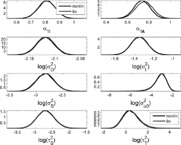
Figure 2: Estimates of marginal densities of nonlinear parameters under nonlinear (solid) and linearized (dashed) versions of the model $M(U=0,\mathit{GST}=0,A=1)$.

Estimates of the marginal posterior densities of $\gamma$ and $w$ are shown in Figure 2 and Figure 6 in the online supplements [Bliznyuk et al. (2014)]. The marginal densities of elements of $\gamma$ and $w$ are remarkably similar between the nonlinear and linearized models, with the exception of the densities of $\gamma_{2}=\alpha_{1A}$; these are still close to one another. Plots of spatial predictions—obtained as means of the posterior predictive distribution—for the two models (Figure 7 in the online supplements [Bliznyuk et al. (2014)]) are also visually indistinguishable, which provides further support for the use of linearization. The correlation between the spatial predictions under the two models is 0.9999 on both the logarithmic and original scale. We also examined the distribution and spatial variability of the pointwise prediction differences. The variability of the differences tends to increase with the distance from the central site monitor (as expected due to the curse of dimensionality), but the predictions are still very close to each other. The relative accuracy of predictions on the original scale, computed pointwise as the absolute value of the differences of the predictions divided by the predicted value under the nonlinear model, is very high. For example, the 90th, 95th, 99th and 99.5th percentiles for the empirical distribution of the relative errors were 0.011, 0.014, 0.033 and 0.040, respectively.

4.4 Bayesian inference and prediction

In this section we report results under the model chosen in Section 4.2, which includes the short-range process, $u$, and the multiday data but excludes the long-range $g_{\mathit{ST}}$ process.

To sample from $[\gamma|Y^{\mathit{OIA}}]$ using the computational strategy of Section 3, we launched four Markov chains, initialized in the region of high posterior probability of $\gamma$. Each chain had a length of 12,500, and a burn-in sample of size 2500 was discarded from each. We examined trace plots of MCMC states and the corresponding posterior density estimates to determine that the chains mixed rapidly and converged to the same posterior.

=213pt Parameter Mean 2.5% 50% 97.5% $\alpha_{1I}$ 0.956 0.870 0.957 1.040 $\alpha_{1A}$ 0.698 0.576 0.702 0.817 $\sigma_{O}^{2}$ 0.045 0.041 0.045 0.049 $\sigma_{I}^{2}$ 0.129 0.101 0.125 0.161 $\sigma_{S}^{2}$ 0.037 0.021 0.035 0.056 $\sigma_{\alpha 0}^{2}$ 0.030 0.011 0.024 0.057 $\tau_{S}^{2}$ 0.030 0.016 0.027 0.047 $\tau_{T}^{2}$ 2.774 0.182 0.974 7.168 $\sigma_{u}^{2}$ 0.098 0.090 0.098 0.106 $\theta_{S}$ 0.054 0.043 0.053 0.066 $\theta_{T}$ 0.120 0.073 0.120 0.169

Table 3: Posterior summaries of nonlinear parameters under model $M(U=1,\mathit{GST}=0,A=1)$

Posterior means and quantiles for $\gamma$ are given in Table 3. Even though parameters $\alpha_{1I}$ and $\alpha_{1A}$ have similar interpretations, $\alpha_{1A}$ is smaller in magnitude than $\alpha_{1I}$. This suggests that multiday indoor data are less informative for daily predictions of the outdoor exposure process than daily indoor data. This is plausible because readings from 30 out of 45 BCI sites overlap spatially and temporally with those from BCO sites, whereas all BCA sites are spatially and often temporally disjoint from the BCO sites. Consequently, the spatio-temporal mismatch causes measurement error in the regressor (the latent process here), and the coefficients are shrunk more toward zero whenever there is more error in the covariate. The temporal decay parameter $\theta_{T}\approx 0.12$, interpreted in light of the tapering structure, corresponds to a model with temporal correlation function that is about 0.7 at lag one but decays faster than that of the $\mathit{AR}(1)$ process with lag-one correlation of 0.7. The spatial decay parameter $\theta_{S}\approx 0.054$ (on the 1 km distance scale) corresponds to spatial correlation that decays to 0.05 by about 35 km. Consequently, when predicting within the temporal range of measurements, the short-range process, $u$, “pulls” the predictions toward the observed data, thereby capturing the nonperiodic features of the exposure process not accounted for by $\zeta$.

Posterior means and quantiles for the coefficients of the observable covariates are reported in Table 1. Based on preliminary exploratory analysis using only the outdoor data, the logarithm of readings from the central site monitor (logHSPH) was the most important covariate for spatio-temporal prediction. From the Bayesian model fit using data from all sources, this conjecture was further supported by the relative widths and quantiles of the credible intervals. The effect of other temporally-varying covariates such as wind speed and the planetary boundary layer is not easily interpretable in the presence of interactions of spatial and temporal covariates. However, certain two- and three-way interactions have been shown to add to the predictive ability of other prediction models in the Boston area [Zanobetti et al. (2014)]. The spatially-varying population and land use covariates are positively associated with the response. The traffic density covariate is of most interest because of the relationship between black carbon and traffic that motivates this work. Its marginal effect—once the interactions with temporally varying covariates have been accounted for—is positive, which can be clearly seen in Figure 3, in which predictions follow the road network. In the early phase of this project we considered models with fewer predictors and without interactions, which yielded a similar relative ranking of the models and slightly less accurate predictions.

Figure 3: Log black carbon predictions for July 31, 2006 based on the mean of the predictive distribution, $E(\eta^{P}|Y^{\mathit{OIA}})$, under the final model $M(U=1,\mathit{GST}=0,A=1)$. The unit is the natural logarithm of $\mu g/m^{3}$.

The primary goal of our work is to predict a vector of latent process values, $\eta^{P}$, in the region for any temporal period of interest for health effects analysis, which is done using $E(\eta^{P}|Y^{\mathit{OIA}})$. Because of the temporal covariance tapering, if the minimum distance between the temporal indices in $\eta^{P}$ and in $Y^{\mathit{OIA}}$ exceeds the range of the taper function, then $E(\eta^{P}|Y^{\mathit{OIA}})=E(C^{P}w|Y^{\mathit{OIA}})$, where $C^{P}$ is the “design matrix” for $\eta^{P}$. Figure 3 shows predictions for an example day (July 31, 2006) based on the MCMC estimate of $E(\eta^{P}|Y^{\mathit{OIA}})$.

5 Discussion

In this paper we developed a unified exposure prediction framework that aggregates air pollutant concentration data from multiple disparate sources that are available at different levels of temporal resolution, which is of great importance for health effects models arising in environmental science. We found that incorporation of even a modest number of observations (93 or under 1.5% of the overall observation count) of the multiday data from a relatively large spatial network (roughly doubling the number of unique spatial sites) uniformly improves the prediction quality in a number of models that may or may not include long-term and short-term spatio-temporal signal. To our surprise, incorporation of a periodic long-range spatio-temporal trend did not produce considerable improvements over the models without the long-range interaction. We attribute this to the fact that the air monitors in the networks corresponding to each study are scattered in space and operate irregularly in time, which implies that the observed data correspond to under 5% of the dates from all the monitors over the whole study period. In our models, the departures from the periodic trend are being captured by the short-range process. If the temporal coverage were richer, we would be able to identify the nonperiodic component of long-range variability better and to rigorously test its presence.

Our linearization approach provides a computationally efficient means to build two quadratic approximations: (i) the logarithm of $[\eta^{A}|v,\gamma,Y^{\mathit{OIA}}]$ and (ii) the logarithm of $[\eta^{A},\eta^{P}|v,\gamma,Y^{\mathit{OIA}}]$, where $\eta^{P}$ is a vector of latent process values we want to predict. This produces a linearized model with Gaussian approximations for the marginal likelihood and required conditional posterior densities. An alternative that also results in Gaussian approximations is to approximate (i) and (ii) using a two-term Taylor expansion about the appropriate modes, which needs to be located by a costly optimization run. Using these approximations to integrate out $\eta^{A}$ is equivalent to the Laplace approximation [Tierney and Kadane (1986)]. The downside of this scheme is that the approximation needs to be built for every value of $(v,\gamma)$ of interest, which is infeasible in practice.

While we adopt an MCMC-based approach to Bayesian inference and prediction, a promising direction for future work is to consider an approximation scheme in the spirit of Rue, Martino and Chopin (2009), the integrated nested Laplace approximation (INLA). Methodologically, one will need to address the following two issues that are critical to the computational performance of INLA for inference in latent process models that combine multiple data sets, both in our case study and in general. First, one needs to be able to enforce the Markov property of the spatio-temporal latent process. Second, increasing the number of data sets in the joint model (that are linked by the latent process) and the complexity of the model for the latent process adds to the dimension of the hyperparameter vector $\gamma$ [$\bolds{\theta}$ in Rue, Martino and Chopin (2009)], which can make accurate numerical integration computationally demanding, if feasible.

References

- Adar et al. (2010) {barticle}[auto:STB—2014/06/18—12:29:53] \bauthor\bsnmAdar, \bfnmS. D.\binitsS. D., \bauthor\bsnmKlein, \bfnmR.\binitsR., \bauthor\bsnmKlein, \bfnmB. E. K.\binitsB. E. K., \bauthor\bsnmSzpiro, \bfnmA. A.\binitsA. A., \bauthor\bsnmCotch, \bfnmM. F.\binitsM. F., \bauthor\bsnmWong, \bfnmT. Y.\binitsT. Y., \bauthor\bsnmO’Neill, \bfnmM. S.\binitsM. S., \bauthor\bsnmShrager, \bfnmS.\binitsS., \bauthor\bsnmBarr, \bfnmR. G.\binitsR. G., \bauthor\bsnmSiscovick, \bfnmD. S.\binitsD. S., \bauthor\bsnmDaviglus, \bfnmM. L.\binitsM. L., \bauthor\bsnmSampson, \bfnmP. D.\binitsP. D. and \bauthor\bsnmKaufman, \bfnmJ. D.\binitsJ. D. (\byear2010). \btitleAir pollution and the microvasculature: A cross-sectional assessment of in vivo retinal images in the population-based multi-ethnic study of atherosclerosis (MESA). \bjournalPLOS Medicine \bvolume7 \bpagese1000372. \bptokimsref\endbibitem
- Banerjee, Carlin and Gelfand (2004) {bbook}[auto:STB—2014/06/18—12:29:53] \bauthor\bsnmBanerjee, \bfnmS.\binitsS., \bauthor\bsnmCarlin, \bfnmB. P.\binitsB. P. and \bauthor\bsnmGelfand, \bfnmA. E.\binitsA. E. (\byear2004). \btitleHierarchical Modeling and Analysis for Spatial Data. \bpublisherChapman & Hall, \blocationBoca Raton, FL. \bptokimsref\endbibitem
- Berhane et al. (2004) {barticle}[mr] \bauthor\bsnmBerhane, \bfnmKiros\binitsK., \bauthor\bsnmGauderman, \bfnmW. James\binitsW. J., \bauthor\bsnmStram, \bfnmDaniel O.\binitsD. O. and \bauthor\bsnmThomas, \bfnmDuncan C.\binitsD. C. (\byear2004). \btitleStatistical issues in studies of the long-term effects of air pollution: The Southern California children’s health study. \bjournalStatist. Sci. \bvolume19 \bpages414–449. \biddoi=10.1214/088342304000000413, issn=0883-4237, mr=2185625 \bptnotecheck related \bptokimsref\endbibitem
- Bliznyuk, Ruppert and Shoemaker (2011) {barticle}[mr] \bauthor\bsnmBliznyuk, \bfnmNikolay\binitsN., \bauthor\bsnmRuppert, \bfnmDavid\binitsD. and \bauthor\bsnmShoemaker, \bfnmChristine A.\binitsC. A. (\byear2011). \btitleEfficient interpolation of computationally expensive posterior densities with variable parameter costs. \bjournalJ. Comput. Graph. Statist. \bvolume20 \bpages636–655. \biddoi=10.1198/jcgs.2011.09212, issn=1061-8600, mr=2878994 \bptokimsref\endbibitem
- Bliznyuk et al. (2014) {bmisc}[auto:STB—2014/06/18—12:29:53] \bauthor\bsnmBliznyuk, \bfnmNikolay\binitsN., \bauthor\bsnmPaciorek, \bfnmChristopher J.\binitsC. J., \bauthor\bsnmSchwartz, \bfnmJoel\binitsJ. and \bauthor\bsnmCoull, \bfnmBrent\binitsB. (\byear2014). \bhowpublishedSupplement to “Nonlinear predictive latent process models for integrating spatio-temporal exposure data from multiple sources.” DOI:\doiurl10.1214/14-AOAS737SUPP. \bptokimsref \endbibitem
- Calder (2007) {barticle}[mr] \bauthor\bsnmCalder, \bfnmCatherine A.\binitsC. A. (\byear2007). \btitleDynamic factor process convolution models for multivariate space–time data with application to air quality assessment. \bjournalEnviron. Ecol. Stat. \bvolume14 \bpages229–247. \biddoi=10.1007/s10651-007-0019-y, issn=1352-8505, mr=2405328 \bptokimsref\endbibitem
- Calder (2008) {barticle}[mr] \bauthor\bsnmCalder, \bfnmCatherine A.\binitsC. A. (\byear2008). \btitleA dynamic process convolution approach to modeling ambient particulate matter concentrations. \bjournalEnvironmetrics \bvolume19 \bpages39–48. \biddoi=10.1002/env.852, issn=1180-4009, mr=2416543 \bptokimsref\endbibitem
- Christensen, Roberts and Sköld (2006) {barticle}[mr] \bauthor\bsnmChristensen, \bfnmOle F.\binitsO. F., \bauthor\bsnmRoberts, \bfnmGareth O.\binitsG. O. and \bauthor\bsnmSköld, \bfnmMartin\binitsM. (\byear2006). \btitleRobust Markov chain Monte Carlo methods for spatial generalized linear mixed models. \bjournalJ. Comput. Graph. Statist. \bvolume15 \bpages1–17. \biddoi=10.1198/106186006X100470, issn=1061-8600, mr=2269360 \bptokimsref\endbibitem
- Christensen and Waagepetersen (2002) {barticle}[mr] \bauthor\bsnmChristensen, \bfnmOle F.\binitsO. F. and \bauthor\bsnmWaagepetersen, \bfnmRasmus\binitsR. (\byear2002). \btitleBayesian prediction of spatial count data using generalized linear mixed models. \bjournalBiometrics \bvolume58 \bpages280–286. \biddoi=10.1111/j.0006-341X.2002.00280.x, issn=0006-341X, mr=1908167 \bptokimsref\endbibitem
- Fuentes and Raftery (2005) {barticle}[mr] \bauthor\bsnmFuentes, \bfnmMontserrat\binitsM. and \bauthor\bsnmRaftery, \bfnmAdrian E.\binitsA. E. (\byear2005). \btitleModel evaluation and spatial interpolation by Bayesian combination of observations with outputs from numerical models. \bjournalBiometrics \bvolume61 \bpages36–45. \biddoi=10.1111/j.0006-341X.2005.030821.x, issn=0006-341X, mr=2129199 \bptokimsref\endbibitem
- Furrer, Genton and Nychka (2006) {barticle}[mr] \bauthor\bsnmFurrer, \bfnmReinhard\binitsR., \bauthor\bsnmGenton, \bfnmMarc G.\binitsM. G. and \bauthor\bsnmNychka, \bfnmDouglas\binitsD. (\byear2006). \btitleCovariance tapering for interpolation of large spatial datasets. \bjournalJ. Comput. Graph. Statist. \bvolume15 \bpages502–523. \biddoi=10.1198/106186006X132178, issn=1061-8600, mr=2291261 \bptokimsref\endbibitem
- Gelfand, Zhu and Carlin (2001) {barticle}[auto:STB—2014/06/18—12:29:53] \bauthor\bsnmGelfand, \bfnmA.\binitsA., \bauthor\bsnmZhu, \bfnmL.\binitsL. and \bauthor\bsnmCarlin, \bfnmB.\binitsB. (\byear2001). \btitleOn the change of support problem for spatio-temporal data. \bjournalBiostatistics \bvolume2 \bpages31–45. \bptokimsref\endbibitem
- Gneiting and Raftery (2007) {barticle}[mr] \bauthor\bsnmGneiting, \bfnmTilmann\binitsT. and \bauthor\bsnmRaftery, \bfnmAdrian E.\binitsA. E. (\byear2007). \btitleStrictly proper scoring rules, prediction, and estimation. \bjournalJ. Amer. Statist. Assoc. \bvolume102 \bpages359–378. \biddoi=10.1198/016214506000001437, issn=0162-1459, mr=2345548 \bptokimsref\endbibitem
- Gneiting, Ševčíková and Percival (2012) {barticle}[mr] \bauthor\bsnmGneiting, \bfnmTilmann\binitsT., \bauthor\bsnmŠevčíková, \bfnmHana\binitsH. and \bauthor\bsnmPercival, \bfnmDonald B.\binitsD. B. (\byear2012). \btitleEstimators of fractal dimension: Assessing the roughness of time series and spatial data. \bjournalStatist. Sci. \bvolume27 \bpages247–277. \biddoi=10.1214/11-STS370, issn=0883-4237, mr=2963995 \bptokimsref\endbibitem
- Golub and Van Loan (1996) {bbook}[mr] \bauthor\bsnmGolub, \bfnmGene H.\binitsG. H. and \bauthor\bsnmVan Loan, \bfnmCharles F.\binitsC. F. (\byear1996). \btitleMatrix Computations, \bedition3rd ed. \bpublisherJohns Hopkins Univ. Press, \blocationBaltimore, MD. \bidmr=1417720 \bptokimsref\endbibitem
- Gotway and Young (2002) {barticle}[mr] \bauthor\bsnmGotway, \bfnmCarol A.\binitsC. A. and \bauthor\bsnmYoung, \bfnmLinda J.\binitsL. J. (\byear2002). \btitleCombining incompatible spatial data. \bjournalJ. Amer. Statist. Assoc. \bvolume97 \bpages632–648. \biddoi=10.1198/016214502760047140, issn=0162-1459, mr=1951636 \bptokimsref\endbibitem
- Gotway and Young (2007) {barticle}[mr] \bauthor\bsnmGotway, \bfnmCarol A.\binitsC. A. and \bauthor\bsnmYoung, \bfnmLinda J.\binitsL. J. (\byear2007). \btitleA geostatistical approach to linking geographically aggregated data from different sources. \bjournalJ. Comput. Graph. Statist. \bvolume16 \bpages115–135. \biddoi=10.1198/106186007X179257, issn=1061-8600, mr=2345750 \bptokimsref\endbibitem
- Gryparis et al. (2007) {barticle}[mr] \bauthor\bsnmGryparis, \bfnmAlexandros\binitsA., \bauthor\bsnmCoull, \bfnmBrent A.\binitsB. A., \bauthor\bsnmSchwartz, \bfnmJoel\binitsJ. and \bauthor\bsnmSuh, \bfnmHelen H.\binitsH. H. (\byear2007). \btitleSemiparametric latent variable regression models for spatiotemporal modelling of mobile source particles in the greater Boston area. \bjournalJ. Roy. Statist. Soc. Ser. C \bvolume56 \bpages183–209. \biddoi=10.1111/j.1467-9876.2007.00573.x, issn=0035-9254, mr=2359241 \bptokimsref\endbibitem
- Gryparis et al. (2009) {barticle}[pbm] \bauthor\bsnmGryparis, \bfnmAlexandros\binitsA., \bauthor\bsnmPaciorek, \bfnmChristopher J.\binitsC. J., \bauthor\bsnmZeka, \bfnmAriana\binitsA., \bauthor\bsnmSchwartz, \bfnmJoel\binitsJ. and \bauthor\bsnmCoull, \bfnmBrent A.\binitsB. A. (\byear2009). \btitleMeasurement error caused by spatial misalignment in environmental epidemiology. \bjournalBiostatistics \bvolume10 \bpages258–274. \biddoi=10.1093/biostatistics/kxn033, issn=1468-4357, pii=kxn033, pmcid=2733173, pmid=18927119 \bptokimsref\endbibitem
- Haario, Saksman and Tamminen (2001) {barticle}[mr] \bauthor\bsnmHaario, \bfnmHeikki\binitsH., \bauthor\bsnmSaksman, \bfnmEero\binitsE. and \bauthor\bsnmTamminen, \bfnmJohanna\binitsJ. (\byear2001). \btitleAn adaptive Metropolis algorithm. \bjournalBernoulli \bvolume7 \bpages223–242. \biddoi=10.2307/3318737, issn=1350-7265, mr=1828504 \bptokimsref\endbibitem
- Janssen et al. (2011) {barticle}[auto:STB—2014/06/18—12:29:53] \bauthor\bsnmJanssen, \bfnmN. A. H.\binitsN. A. H., \bauthor\bsnmHoek, \bfnmG.\binitsG., \bauthor\bsnmSimic-Lawson, \bfnmS.\binitsS., \bauthor\bsnmFischer, \bfnmP.\binitsP., \bauthor\bsnmvan Bree, \bfnmL.\binitsL., \bauthor\bsnmten Brink, \bfnmH.\binitsH., \bauthor\bsnmKeuken, \bfnmM.\binitsM., \bauthor\bsnmAtkinson, \bfnmR. W.\binitsR. W., \bauthor\bsnmAnderson, \bfnmH. R.\binitsH. R., \bauthor\bsnmBrunekreef, \bfnmB.\binitsB. and \bauthor\bsnmCasee, \bfnmF. R.\binitsF. R. (\byear2011). \btitleBlack carbon as an additional indicator of the adverse health effects of airborne particles compared with PM10 and PM2.5. \bjournalEnviron. Health Perspect. \bvolume119 \bpages1691–1699. \bptokimsref\endbibitem
- Opsomer, Wang and Yang (2001) {barticle}[mr] \bauthor\bsnmOpsomer, \bfnmJean\binitsJ., \bauthor\bsnmWang, \bfnmYuedong\binitsY. and \bauthor\bsnmYang, \bfnmYuhong\binitsY. (\byear2001). \btitleNonparametric regression with correlated errors. \bjournalStatist. Sci. \bvolume16 \bpages134–153. \biddoi=10.1214/ss/1009213287, issn=0883-4237, mr=1861070 \bptokimsref\endbibitem
- Robert and Casella (1999) {bbook}[mr] \bauthor\bsnmRobert, \bfnmChristian P.\binitsC. P. and \bauthor\bsnmCasella, \bfnmGeorge\binitsG. (\byear1999). \btitleMonte Carlo Statistical Methods. \bpublisherSpringer, \blocationNew York. \biddoi=10.1007/978-1-4757-3071-5, mr=1707311 \bptokimsref\endbibitem
- Rue and Held (2005) {bbook}[mr] \bauthor\bsnmRue, \bfnmHåvard\binitsH. and \bauthor\bsnmHeld, \bfnmLeonhard\binitsL. (\byear2005). \btitleGaussian Markov Random Fields: Theory and Applications. \bseriesMonographs on Statistics and Applied Probability \bvolume104. \bpublisherChapman & Hall, \blocationBoca Raton, FL. \biddoi=10.1201/9780203492024, mr=2130347 \bptokimsref\endbibitem
- Rue, Martino and Chopin (2009) {barticle}[mr] \bauthor\bsnmRue, \bfnmHåvard\binitsH., \bauthor\bsnmMartino, \bfnmSara\binitsS. and \bauthor\bsnmChopin, \bfnmNicolas\binitsN. (\byear2009). \btitleApproximate Bayesian inference for latent Gaussian models by using integrated nested Laplace approximations. \bjournalJ. R. Stat. Soc. Ser. B Stat. Methodol. \bvolume71 \bpages319–392. \biddoi=10.1111/j.1467-9868.2008.00700.x, issn=1369-7412, mr=2649602 \bptokimsref\endbibitem
- Ruppert, Wand and Carroll (2003) {bbook}[mr] \bauthor\bsnmRuppert, \bfnmDavid\binitsD., \bauthor\bsnmWand, \bfnmM. P.\binitsM. P. and \bauthor\bsnmCarroll, \bfnmR. J.\binitsR. J. (\byear2003). \btitleSemiparametric Regression. \bpublisherCambridge Univ. Press, \blocationCambridge. \biddoi=10.1017/CBO9780511755453, mr=1998720 \bptokimsref\endbibitem
- Tierney and Kadane (1986) {barticle}[mr] \bauthor\bsnmTierney, \bfnmLuke\binitsL. and \bauthor\bsnmKadane, \bfnmJoseph B.\binitsJ. B. (\byear1986). \btitleAccurate approximations for posterior moments and marginal densities. \bjournalJ. Amer. Statist. Assoc. \bvolume81 \bpages82–86. \bidissn=0162-1459, mr=0830567 \bptokimsref\endbibitem
- van Dyk and Park (2008) {barticle}[mr] \bauthor\bparticlevan \bsnmDyk, \bfnmDavid A.\binitsD. A. and \bauthor\bsnmPark, \bfnmTaeyoung\binitsT. (\byear2008). \btitlePartially collapsed Gibbs samplers: Theory and methods. \bjournalJ. Amer. Statist. Assoc. \bvolume103 \bpages790–796. \biddoi=10.1198/016214508000000409, issn=0162-1459, mr=2524010 \bptokimsref\endbibitem
- Wang (1998) {barticle}[auto:STB—2014/06/18—12:29:53] \bauthor\bsnmWang, \bfnmY.\binitsY. (\byear1998). \btitleSmoothing spline models with correlated random errors. \bjournalJ. Amer. Statist. Assoc. \bvolume93 \bpages341–348. \bptokimsref\endbibitem
- Wannemuehler et al. (2009) {barticle}[mr] \bauthor\bsnmWannemuehler, \bfnmKathleen A.\binitsK. A., \bauthor\bsnmLyles, \bfnmRobert H.\binitsR. H., \bauthor\bsnmWaller, \bfnmLance A.\binitsL. A., \bauthor\bsnmHoekstra, \bfnmRobert M.\binitsR. M., \bauthor\bsnmKlein, \bfnmMitchel\binitsM. and \bauthor\bsnmTolbert, \bfnmPaige\binitsP. (\byear2009). \btitleA conditional expectation approach for associating ambient air pollutant exposures with health outcomes. \bjournalEnvironmetrics \bvolume20 \bpages877–894. \biddoi=10.1002/env.978, issn=1180-4009, mr=2838493 \bptokimsref\endbibitem
- Wood (2006) {bbook}[mr] \bauthor\bsnmWood, \bfnmSimon N.\binitsS. N. (\byear2006). \btitleGeneralized Additive Models: An Introduction with . \bpublisherChapman & Hall, \blocationBoca Raton, FL. \bidmr=2206355 \bptokimsref\endbibitem
- Zanobetti et al. (2014) {barticle}[auto:STB—2014/06/18—12:29:53] \bauthor\bsnmZanobetti, \bfnmA.\binitsA., \bauthor\bsnmCoull, \bfnmB. A.\binitsB. A., \bauthor\bsnmGryparis, \bfnmA.\binitsA., \bauthor\bsnmSparrow, \bfnmD.\binitsD., \bauthor\bsnmVokonas, \bfnmP. S.\binitsP. S., \bauthor\bsnmWright, \bfnmR. O.\binitsR. O., \bauthor\bsnmGold, \bfnmD. R.\binitsD. R. and \bauthor\bsnmSchwartz, \bfnmJ.\binitsJ. (\byear2014). \btitleAssociations between arrhythmia episodes and temporally and spatially resolved black carbon and particulate matter in elderly patients. \bjournalOccup. Environ. Med. \bvolume71 \bpages201–207. \bptokimsref\endbibitem
- Zeger et al. (2000) {barticle}[auto:STB—2014/06/18—12:29:53] \bauthor\bsnmZeger, \bfnmS. L.\binitsS. L., \bauthor\bsnmThomas, \bfnmD.\binitsD., \bauthor\bsnmDominici, \bfnmF.\binitsF., \bauthor\bsnmSamet, \bfnmJ. M.\binitsJ. M., \bauthor\bsnmSchwartz, \bfnmJ.\binitsJ., \bauthor\bsnmDockery, \bfnmD.\binitsD. and \bauthor\bsnmCohen, \bfnmA.\binitsA. (\byear2000). \btitleExposure measurement error in time-series studies of air pollution: Concepts and consequences. \bjournalOccup. Environ. Med. \bvolume108 \bpages419–426. \bptokimsref\endbibitem