Growing Scale-free Networks by a Mediation-Driven Attachment Rule

Abstract

We propose a model that generates a class of networks exhibiting power-law degree distribution with a spectrum of exponents depending on the number of links ($m$) with which incoming nodes join the existing network. Here, each new node first picks an existing node at random, and connects not with this but with $m$ of its neighbors also picked at random. Counter-intuitively enough, such a mediation-driven attachment rule gives rise to superhubs for small $m$ due to the winners take all effect, and hubs for large $m$ due to the winners take some effect. To solve it analytically, we use mean-field approximation where we find that the inverse harmonic mean of degrees of the neighborhood of each existing node and their mean play a crucial role in determining the quality of the degree distribution.

In the recent past, we have amassed a bewildering amount of information on our universe, and yet we are far from developing a holistic idea. This is because most of the natural and man-made real-world systems are intricately wired and seemingly complex. Much of these complex systems can be mapped as networks consisting of nodes connected by links, e.g., author collaboration and movie actor networks, the Internet, World Wide Web, neural and protein networks etc. ref.coauthorship ; ref.movieactor_2 ; ref.internet ; ref.www ; ref.brain ; ref.protein . While working on some of these real-world systems Barabási and Albert (BA) in late $90$s found that the tail of the degree distribution $P(k)$, the probability that a randomly chosen node is connected to $k$ other nodes, always follows a power-law. In pursuit of theoretical explanation they realized that real networks are not static, rather they grow. They also realized that a new node does not connect with an existing one randomly rather preferentially with respect to their degrees - which is now known as the preferential attachment (PA) rule ref.barabasi . Incorporating both the ingredients BA proposed a model and showed that it exhibits power-law degree distribution $P(k)\sim k^{-\gamma}$ where $\gamma=3$. Despite the profound success of the BA model we are compelled to note a couple of drawbacks. First and foremost, the preferential attachment (PA) rule is too direct. Second, the BA model can only account for $\gamma=3$ while in real networks the exponent $\gamma$ assumes a spectrum of values between $2<\gamma\leq 3$. To overcome these drawbacks there exist a few variants of the BA model through the inclusion of rewiring, aging, ranking etc. ref.rewiring ; ref.rewiring_1 ; ref.aging_1 ; ref.ranking , and a few alternatives to the direct PA mechanism like redirection, vertex copying, and duplication mechanisms ref.redirection_sublinear ; ref.hi_dispersed ; ref.copying ; ref.duplication .

(a)

(b)

Figure 1: Snapshots of networks grown using (a) the PA rule of the BA model and (b) the MDA rule. The size of each node is drawn according to its degree showing that the hubs of networks grown using the MDA rule are richer than those of the BA networks.

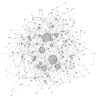
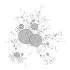
In this article, we propose a model in which a walker is parachuted to an arbitrary node of the existing network at random and then takes a random step to one of its neighbors. The new node is attached to the node where the walker stops. The model has been inspired by the growth of the weighted planar stochastic lattice (WPSL) ref.hassan_njp ; ref.hassan_conf . Seeing its dual emerges as a scale-free network, we became curious as to what happens when a graph is grown following a similar rule. That is, an existing node connects with the incoming node only if one of its neighbors is picked at random. We call it the mediation-driven attachment (MDA) rule since the node where the walker first landed acts as a mediator for connection between its neighbor and the new node. We use mean-field approximation (MFA) to solve the model analytically, and use numerical simulation to verify the solution. We show that for small $m$, the MDA rule is super-preferential due to winners take all (WTA) effect that gives rise to a few superhubs. The snapshots of the networks grown according to BA and MDA rules shown in FIG. 1 for $m=2$ clearly reveal the presence of hubs and superhubs respectively. However, for large $m$ the WTA effect is replaced by winners take some (WTS) effect that gives rise to simple hubs only. The essential idea of the MDA rule can be seen in the formation of trade links among businessmen and in the growth of the WWW. In business, a newcomer wishing to establish trade links with other businessmen can never assess the whole network to see who has how many links in order to decide who will be his partner, owing to the large size of the trade world. Instead, he uses a mediator to find a suitable partner. We note that there exist a couple of works similar to our model albeit the ensuing analysis and the results are completely different from ours ref.mda_1 ; ref.mda_2 ; ref.redirection .

Figure 2: A schematic description of the MDA rule.

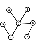
To illustrate the MDA rule we consider a miniature network in FIG. 2 consisting of $m_{0}=6$ nodes labeled $i=1,2,...,6$. This can be considered as the seed. Now to connect a new node to it, we first pick a node at random from the $6$ existing nodes, say node $2$. Second, we pick one of its four neighbors, also with equal a priori probability, say it is node $6$, and connect it with the new node which we label $7$. In this particular example we assume that the new nodes are born with one link or edge, i.e. $m=1$. In the case of new nodes arriving with more than one edge we first pick one node randomly from the entire network followed by picking $m$ of its distinct neighbors and connect them with $m$ new edges. Now the question is, according to our model, what is the probability $\Pi(i)$ that an existing node $i$ is finally picked and the new node gets connected with it? Say, the node $i$ has degree $k_{i}$ and its $k_{i}$ neighbors, labeled $1,2,\ldots,k_{i}$, have degrees $k_{1},k_{2},...,k_{k_{i}}$ respectively. We can reach the node $i$ from each of these $k_{i}$ nodes with probabilities inverse of their respective degrees, and each of the $k_{i}$ nodes can be picked at random with probability $1/N$. We can therefore write

$$\Pi(i)=\frac{1}{N}\Big{[}\frac{1}{k_{1}}+\frac{1}{k_{2}}+\ldots+\frac{1}{k_{k_{i}}}\Big{]}=\frac{\sum_{j=1}^{k_{i}}{\frac{1}{k_{j}}}}{N}.$$ (1)

The probabilities $\Pi(i)$ are normalized, which implies that $\sum_{i=1}^{N}\sum_{j=1}^{k_{i}}{\frac{1}{k_{j}}}=N$. We have verified it numerically and found that it is independent of $m$ and $N$. The rate at which an arbitrary node $i$ gains links is therefore given by the following rate equation.

$${\frac{\partial k_{i}}{\partial t}}=m\ \Pi(i)$$ (2)

The factor $m$ takes care of the fact that any of the $m$ links of the newcomer may connect with the node $i$.

Figure 3: The distribution of IHM for different $m$ values. The fluctuations of IHM of individual nodes is shown in the inset (top left for $m=1$ and bottom right for $m=100$).

Solving Eq.(2) for $\Pi(i)$ given by Eq.(1) seems quite a formidable task unless we can simplify it in some way. A few steps of hand calculation on a network of small size reveals that the probability $\Pi(i)$ of picking node $i$ is higher for nodes with higher degree than those with lower degree, encouraging us to re-write Eq.(1) as

$$\ \Pi(i)=\frac{k_{i}}{N}\ \frac{\sum_{j=1}^{k_{i}}{\frac{1}{k_{j}}}}{k_{i}}.$$ (3)

The factor $\frac{\sum_{j=1}^{k_{i}}{\frac{1}{k_{j}}}}{k_{i}}$ is the inverse of the harmonic mean (IHM) of degrees of the $k_{i}$ neighbors of a node $i$ which we denote as $\Big{<}\frac{1}{k_{i}}\Big{>}$ for convenience. We now attempt to replace the IHM value of each node by an effective “mean value”

$$\Big{<}{\frac{1}{k_{i}}}\Big{>}\approx\overline{\Big{<}{\frac{1}{k_{i}}}\Big{>}},$$ (4)

where the overline indicates the ensemble average of the mean IHM of each realization. In this way, all the information on correlations in the fluctuations is lost and hence we call it mean-field approximation (MFA). One immediate consequence is that like the BA model, our MDA rule too is preferential in character. This may sound a bit too drastic at this stage, but we shall justify it anyway. It is needless to mention that this approximation will work only if the fluctuations of IHM of individual nodes from their mean is not wild.

Figure 4: Plot of $m\overline{\Big{<}{\frac{1}{k_{i}}}\Big{>}}\equiv\beta(m,N)$ vs. $N$ for $m=70$. Inset shows that $\beta(m,N)$ saturates to $\beta(m,\infty)=0.490513$ algebraically as $N^{-3/5}$.

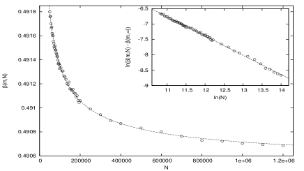
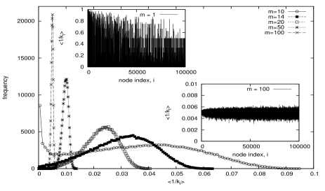
We perform extensive numerical simulation to check how robust the approximation is. For that we calculate the IHM for each node of the network grown with fixed $m$, and plot them as a function of node label $i=1,2,...,N$ (as in the insets of FIG. 3). We find that for small values of $m$, the data points fluctuate so wildly from node to node that the mean of $\Big{<}{\frac{1}{k_{i}}}\Big{>}$ over the entire size of the network bears no meaning, which can also be seen from the frequency distributions of IHM shown in FIG. 3. The frequency distributions become symmetric as we increase $m$ approximately beyond $14$, and the fluctuations occur at increasingly lesser extents, and hence the meaning of the mean seems to be more meaningful. We also find that the mean of the IHM depends on $m$ and is independent of network size $N$ in the limit $N\rightarrow\infty$ (as demonstrated in FIG. 4). So, we can write for $m>14$,

$$\Pi(i)\approx\frac{k_{i}}{N}\ \overline{\Big{<}{\frac{1}{k_{i}}}\Big{>}}=\frac{k_{i}}{N}\ \frac{\beta(m)}{m},$$ (5)

where the factor $m$ in the denominator is introduced for future convenience. Thus the value of $\beta(m)$ for each fixed $m$ is also independent of $N$ as $N\rightarrow\infty$. Eq.(5) confirms that the attachment probability $\Pi(i)\propto k_{i}$, and hence like the BA model our model too is preferential in character, but not directly.

Figure 5: Plots of $\ln(k_{i})$ versus $\ln(t)$ for $5$ nodes added at five different times for $m=2$. In the inset, we show variation of the slope $\beta$ with $m$.

It is noteworthy that the size $N$ of the network is an indicative of time $t$ since we assume that only one node joins the network at each time step. Thus, for $N>>m_{0}$ we can write $N\sim t$. We can now solve the rate equation. Using Eq.(5) and $N\sim t$ in Eq.(2) we find that the rate equation we ought to solve is

$${\frac{\partial k_{i}}{\partial t}}=k_{i}\ \frac{\beta(m)}{t}.$$ (6)

Solving it subject to the initial condition that the $i$th node is born at time $t=t_{i}$ with $k_{i}(t_{i})=m$ we get,

$$k_{i}(t)=m\Big{(}{\frac{t}{t_{i}}}\Big{)}^{\beta(m)}.$$ (7)

The form of the solution is exactly the same as that of the BA model ref.barabasi except for the $\beta$ value. To test Eq.(7) we plot $\ln(k_{i})$ versus $ln(t)$ in FIG. 5 for a few randomly selected nodes and find a set of parallel straight lines. It implies that all nodes grow linearly as predicted by Eq.(7). However, in contrast to the BA model, the slope ($\beta$) of the straight lines depends on $m$, asymptotically approaching $0.5$ for large $m$ (see inset of FIG. 5). Also, there is a significant difference between $\beta$ obtained using our approximation $\beta(m)=m\overline{\Big{<}{\frac{1}{k_{i}}}\Big{>}}$, with that obtained from the $\ln(k_{i})$ vs. $\ln(t)$ plots when $m\leq 14$. The difference gets negligible as $m$ is increased and this too is correlated to the increase in the symmetry and decrease in the width of the IHM distributions.

Figure 6: Plots of $\ln(P(k))$ vs $\ln(k)$ for $m=1$, $m=15$ and $m=100$ revealing that the MDA rule gives rise to power-law degree distribution. In the inset we show the variation in the exponent $\gamma$ as a function of $m$.

We can now find the degree distribution $P(k)$ by appreciating the fact that it is related to $P(t_{i})$, the probability with which node $i$ is added to the system at time $t_{i}$, via

$$P(k)\ dk=-P(t_{i})\ dt_{i}.$$ (8)

The minus sign is introduced here to take into account that the smaller the value of $t_{i}$ the larger the degree $k_{i}$. Substituting $P(t_{i})=\frac{1}{N}\sim\frac{1}{t}$ (since new nodes are added to the system at equal interval of time) and the derivative of $t_{i}$ with respect to $k_{i}$ from Eq.(7) in Eq.(8) gives

$$P(k)\sim k^{-\gamma(m)},\>\text{where}\>\>\gamma(m)=\frac{1}{\beta(m)}+1.$$ (9)

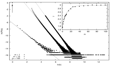
The most immediate difference of this result from that of the BA model is that the exponent $\gamma$ depends on $m$. To verify it we plot in FIG. 6 $\ln(P(k))$ vs. $\ln(k)$ using data extracted from numerical simulation and find straight lines with characteristic fat-tail. This confirms that our analytical solution is in agreement with the numerical solution. It is important to note that for small $m$, especially for $m=1$ there is a special point in the plot of the degree distribution that is way far above the other points. This special point corresponds to $99.5\%$ of the all the nodes which have degree $1$, and which are held by a few hubs. This is reminiscent of the WTA phenomenon. However, as $m$ increases, we find that the WTA phenomenon is replaced by the WTS phenomenon and at the same time, all the data points follow the same trend. This happens when the IHM has less noise and the mean of IHM has meaning. Therefore, we argue that the IHM can be regarded as a measure of how curved or straight the degree distribution is.

The next thing we do is to give a generalized analytical expression for $\gamma$. We fit the data and find that $\gamma$ saturates to $3$ as $\gamma=3(1-0.43531e^{-0.11m})$. The value of $m$ for which $\gamma$ has increased to within a factor of $1-e^{-1}(\approx 63\%)$ of its maximum value $3$, is $m_{c}=\frac{1}{0.11}\approx 9$. We can relate this to the frequency distribution of the IHM in a way that below $m=9$ the distribution is highly asymmetric. From $m=8$ to $m=14$, the distributions gradually metamorphose to assume a Gaussian shape. Also, our numerical simulations show that the whole $\gamma$ spectrum for $m\geq 3$ is between $2$ and $3$. Our result stands in sharp contrast with that of Yang et al. who found the exponent $\gamma$ to vary in the range $1.90$ to $2.61$ when $m$ was varied in the range $1$ to $200$ ref.mda_1 . Besides, our expression for the probability $\Pi$ and method of solution are very different from theirs.

To summarize, we have proposed a new attachment rule, namely the MDA rule, for growing networks that exhibit power-law degree distribution. At a glance, it may seem MDA defies the intuitive idea of the PA rule, however, a closer look reveals otherwise. Indeed, we show explicitly that the MDA rule is in fact not only preferential but superpreferential for $m<14$ and for alrge $m$ it embodies the PA rule but in disguise. We obtained an exact expression for $\Pi(i)$ that describes the probability with which an existing node $i$ is finally picked to be connected with a new node. Solving the model analytically for the exact expression of $\Pi(i)$ appeared to be a formidable task. However, the good news is that we could still find a way to use MFA. Later it turns out that not being able to solve analytically for the exact expression for $\Pi(i)$ was highly rewarding as it helped us gain a deeper insight into the problem. While working with the expression for $\Pi(i)$, we realized that the IHM value of the degrees of the neighborhood of node $i$ plays a crucial role in the model. We find that the fluctuations in IHM values of existing nodes are so wild for small $m$ that the mean, in this case, bears no meaning and hence MFA is not valid in this case. We observed that for small $m$ such as $m=1$ or $2$, the MDA rule becomes super-preferential in the sense that more than $97\%$ of the nodes are extremely poor in degree as they are linked to one or two other nodes which are super-hubs. This is reminiscent of the WTA phenomenon. However, for large $m$, the fluctuations get weaker and their distribution starts to peak around the mean revealing that the mean has a meaning. This is the regime where MFA works well and we verified it numerically. Here we found that the WTA phenomenon is replaced by the WTS phenomenon. We hope to extend our work to study dynamic scaling and universality classes for the MDA model for different $m$ and check how it differs from the BA model ref.mda_data_collapse .

We acknowledge Syed Arefinul Haque for his technical support.

References

- (1) M. E. J. Newman, PNAS 101 5200 (2004).
- (2) M. E. J. Newman, S. H. Strogatz, and D. J. Watts, Phys.Rev. E 64 026118 (2001).
- (3) M. Faloutsos, P. Faloutsos and C. Faloutsos, Comp. Comm. Rev. 29 251 (1999).
- (4) R. Albert, H. Jeong and A. -L. Barabási, Nature 401 130 (1999).
- (5) V. M. Eguiluz, D. R. Chialvo, G. A. Cecchi, M. Baliki and A. V. Apkarian, Phys. Rev. Lett. 94 018102 (2005).
- (6) H. Jeong, S. P. Mason, A. -L. Barabási and Z. N. Oltvai, Nature 411 41 (2001).
- (7) A. -L. Barabási and R. Albert, Science 286 509 (1999).
- (8) R. Albert and A.-L. Barabási, Phys. Rev. Lett. 85 5234 (2000).
- (9) S. S. Manna, A. Kabakcioglu, J. Phys. A: Math. Gen. 36 L279 (2003).
- (10) S.N. Dorogovtsev and J.F.F. Mendes, Phys. Rev. E 62 1842 (2000).
- (11) S. Fortunato, A. Flammini, and F. Menczer, Phys. Rev. Lett. 96 218701 (2006).
- (12) A. Gabel and S. Redner, J. Stat. Mech. 2013 P02043 (2013).
- (13) A. Gabel, P. L. Krapivsky, and S. Redner, Phys. Rev. E 88 050802(R) (2013).
- (14) J. Kim, P. L. Krapivsky, B. Kahng, and S. Redner, Phys. Rev. E 66 055101 (2002).
- (15) F. Chung, L. Lu, T. G. Dewey and , D. J. Galas, J. Computat. Biol. 10 677 (2003).
- (16) M. K. Hassan, M. Z. Hassan and N. I. Pavel, New J. Phys. 12 093045 (2010).
- (17) M. K. Hassan, M. Z. Hassan and N. I. Pavel, Journal of Physics: Conference Series 297 012010 (2011).
- (18) X. -H. Yang, S. -L. Lou, G. Chen, S. -Y. Chen, W. Huang, Physica A 392 3531 (2013).
- (19) S. Boccaletti, D.-U. Hwang and V. Latora, I. J. Bifurcation and Chaos 17 2447 (2007).
- (20) P. L. Krapivsky and S. Redner, Phys. Rev. E 63 066123 (2001).
- (21) M. K. Hassan, M. Z. Hassan and N. I. Pavel, J. Phys A: Math. Theor. 44 175101 (2011).