Post-death Transmission of Ebola:
Challenges for Inference and Opportunities for Control

Abstract

Multiple epidemiological models have been proposed to predict the spread of Ebola in West Africa. These models include consideration of counter-measures meant to slow and, eventually, stop the spread of the disease. Here, we examine one component of Ebola dynamics that is of growing concern – the transmission of Ebola from the dead to the living. We do so by applying the toolkit of mathematical epidemiology to analyze the consequences of post-death transmission. We show that underlying disease parameters cannot be inferred with confidence from early-stage incidence data (that is, they are not “identifiable”) because different parameter combinations can produce virtually the same epidemic trajectory. Despite this identifiability problem, we find robustly that inferences that don’t account for post-death transmission tend to underestimate the basic reproductive number – thus, given the observed rate of epidemic growth, larger amounts of post-death transmission imply larger reproductive numbers. From a control perspective, we explain how improvements in reducing post-death transmission of Ebola may reduce the overall epidemic spread and scope substantially. Increased attention to the proportion of post-death transmission has the potential to aid both in projecting the course of the epidemic and in evaluating a portfolio of control strategies.

Introduction

A recent, influential modeling paper concluded, based on data available as of September 2014, that the ongoing Ebola epidemic in Guinea, Liberia and Sierra Leone had the potential to exceed $1$ million new cases by mid-January 2015, in the absence of intervention meltzer_2014 . Even with intervention and changes in behavior, a follow-up study by an independent group in October 2014 estimated that $100,000$ additional cases could be expected in Liberia alone by mid-December 2014, unless a coordinated, large-scale response is implemented rapidly lewnard_2014 . These predictions leveraged the structure of previous epidemiological models chowell_2004 ; legrand2007understanding that encapsulate the infection cycle of Ebola virus disease (EVD), by tracking the dynamics and interactions of different types of individuals within a population including Susceptible, Exposed, Infectious and Removed types. Exposed individuals are infected but not yet infectious (i.e., also referred to as latently infected). In a SEIR model representation of EVD dynamics, the R class accounts for two types of individuals: those who recovered from the disease and those who have died from the disease (and are therefore “removed”).

However, a complication in modeling EVD arises because EVD may be contracted by direct contact with bodily fluids from individuals who are alive and from those who have died from the disease francesconi_2003 ; CDCEbolaQA2014 . In the present epidemic, contact tracing of 701 individuals confirmed to have been infected with EVD in the ongoing epidemic found that 67 patients reported contacts with individuals who died of EVD, but not with any living EVD cases, while 148 patients reported contacts with both living and dead individuals infected with EVD teamebola , consistent with $10\%=\frac{67}{701}$ to $30\%=\frac{67+148}{701}$ of Ebola cases being caused by post-death transmission. If funerals and burial rites can act as “super-spreader” events lloyd2005 ; galvani2005 ; pandey_2014 , the true fraction may lie outside this range: for example, Legrand and colleagues legrand2007understanding estimated that 2/3 of the total ${\cal{R}}_{0}$ for the 1995 EVD outbreak in the Democratic Republic of Congo could be attributed to post-death transmission. Some early legrand2007understanding and recent (e.g., lewnard_2014 ; pandey_2014 ; gomes2014 ; rivers_2014 ) epidemiological models of EVD have incorporated a D class, thereby distinguishing between recovered and dead individuals. Other models treat post-death transmission implicitly, by increasing the effective transmission rate and/or duration in the I class meltzer_2014 ; althaus2014 . Yet, the implications of post-death transmission for inferences about epidemic spread have not been evaluated systematically. As we show, uncertainty in the relative force of infection before- and after-death has a number of consequences for estimating ${\cal{R}}_{0}$ and the potential for control of the ongoing Ebola epidemic.

Figure 1: Schematic of the SEIRD model, i.e., the dynamics of Susceptible, Exposed (i.e., latently infected), Infectious, Recovered and Dead (but still infectious) individuals. Solid arrows denote transitions between states. Dashed arrows denote that transmission depends on interactions between $S$ and $I$ individuals or between $S$ and $D$ individuals. Parameters $\beta_{I}$ and $\beta_{D}$ are transmission rates, $T_{E}$, $T_{I}$ and $T_{D}$ are the average periods in the $E$, $I$ and $D$ class, respectively, and $f$ is the fraction of individuals who die of EVD.

Results

The basic reproductive number, ${\cal{R}}_{0}$, of EVD includes the effects of post-death transmission

The basic reproductive number, ${\cal{R}}_{0}$, denotes the average number of secondary cases caused by a single infected individual in an otherwise susceptible population. The criterion for epidemic spread in standard epidemiological models is that ${\cal{R}}_{0}>1$ so that the initial infection gives rise, on average, to more than one infected case.

In a conventional SEIR model, EVD transmission between infected and susceptible individuals occurs at an average rate $\beta_{I}$ over a period of infectiousness $T_{I}$. A fraction $f$ of infected individuals die and the remainder, $1-f$, recover and are assumed to be permanently immune to subsequent infection. A SEIRD model includes an additional transmission route: dead individuals can transmit EVD to susceptible individuals at a rate $\beta_{D}$ over a period of infectiousness $T_{D}$, after which they are permanently removed from the system via burial or loss of infectiousness (see Figure  1). Appendix A provides the mathematical details of the model. The basic reproductive number in the SEIRD model is:

$${\cal{R}}_{0}=\beta_{I}T_{I}+f\beta_{D}T_{D}$$ (1)

The first term denotes the average number of secondary infections due to contact with an infected individual before-death. The second term denotes the average number of secondary infectious due to contact with an infected individual after-death. The number of cases arising from contact with dead individuals is modulated by the fraction, $f$, of infected individuals that die due to EVD. In contrast, the basic reproductive number in the SEIR model is:

$${\cal{R}}_{0,SEIR}=\beta_{\mathrm{S}EIR}T_{\mathrm{S}EIR}$$ (2)

It might seem that the basic reproductive number of a SEIRD model should exceed that of a SEIR model. In fact, this will depend on how parameters are estimated. If the SEIR model is fit from data, then $\beta_{\mathrm{S}EIR}$ and $T_{\mathrm{S}EIR}$ will reflect transmission from both living and dead infectious individuals. Thus, we ask: What is the change in the estimated value of ${\cal{R}}_{0}$ given alternative model frameworks meant to explain the same infected case data?

Figure 2: Identifiability problems in inferring epidemiological parameters from early-stage epidemic growth data. (Model) The dynamics are that of an SEIR model (diamond) and SEIRD model (lines and circles) with epidemiological parameters $T_{E}=11$, $T_{I}=6$ and $f=0.7$. For the SEIRD model, three scenarios are considered where $T_{D}=2$, 4 and 6 days. For each scenario, we find various combinations of $\beta_{D}$ and $\beta_{I}$ that lead to the same early-stage epidemic growth rate, $\lambda=1/21$. (Left) The calculated values of $\beta_{I}$, $\beta_{D}$ and ${\cal{R}}_{0}$ (from top-to-bottom) as a function of $\rho_{D}={\cal{R}}_{0}(\mathrm{dead})/{\cal{R}}_{0}$. (Right panel) Dynamics of epidemics for the three highlighted scenarios corresponding to $\beta_{I}=0.05$, 0.15 and 0.25 and $\beta_{D}=0.71$, 0.45 and 0.20 respectively.

Figure 3: Inferring epidemiological parameters from early-stage Ebola epidemic case data in West Africa. (Data) A portion of cumulative case data rivers_github was used to identify an exponential growth rate $\hat{\lambda}$ (see Appendix E). The calibration regime for model fits is denoted in open triangles, where Day 50 is 5/11/14, Day 100 is 6/30/14, Day 150 is 8/19/14 and Day 200 is 10/8/14. (Model) The dynamics are that of an SEIR model (diamond) and SEIRD model (lines and circles) with epidemiological parameters $T_{E}=11$ (modeled as a gamma distribution), $T_{I}=6$ and $f=0.7$. For the SEIRD model, three scenarios are considered where $T_{D}=2$, 4 and 6 days. (Left) The calculated values of $\beta_{I}$, $\beta_{D}$ and ${\cal{R}}_{0}$ (from top-to-bottom) as a function of $\rho_{D}={\cal{R}}_{0}(\mathrm{dead}~{})/{\cal{R}}_{0}$. (Right panel) Dynamics of epidemics for the three highlighted scenarios. For each country, all three scenarios lead to the same country-specific exponential epidemic growth rate, $\hat{\lambda}$.

Identifiability problems in estimating the basic reproductive number, ${\cal{R}}_{0}$

The SEIRD model, like the SEIR, SIR and other epidemiological models, predicts that there should be an exponential increase in the number of infected cases, i.e., $I(t)\sim e^{\lambda t}$, after an initial transient phase and before interventions, large-scale behavioral changes or population-level depletion of susceptibles have taken effect chowell_bmc2014 . The exponential growth rate, $\lambda$, is a function of epidemiological parameters, including the transmission rate and ${\cal{R}}_{0}$ keeling_2007 ; wallinga2007generation . For EVD, prior information is available to constrain the mean duration of the latent phase on the order of 8-12 days eichner2011incubation ; teamebola , the mean infectious period before death or recovery on the order of 5-9 days teamebola ; meltzer_2014 and the fraction of disease-induced mortality of approximately 70% chowell_2004 ; teamebola . However, even with these prior constraints, theory does not predict a one-to-one relationship between ${\cal{R}}_{0}$ – the feature we want to infer – and $\lambda$ – the feature that we can measure. This lack of a one-to-one relationship gives rise to a so-called identifiability problem in estimating epidemiological parameters, including ${\cal{R}}_{0}$, from early-stage epidemic data alone. Appendix C presents a rationale for why identifiability problems arise more generally when fitting epidemiological models.

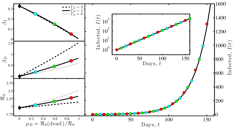
To examine the identifiability problem as it pertains to EVD, we fit both the SEIR and SEIRD models to an exponentially growing epidemic with rate $\hat{\lambda}$ for which the number of cases is increasing with a characteristic time of $1/\hat{\lambda}=21$ days. Further, we assume that $T_{E}=11$ days, $T_{I}=6$ days and $f=0.7$. We utilize standard epidemiological methods to infer ${\cal{R}}_{0}$ for the SEIR model and, in turn, $\beta_{\mathrm{S}EIR}$, given observations of $\hat{\lambda}$ (see Eq. 10). We find a point estimate of $\beta_{\mathrm{S}EIR}$ of 0.33 and a corresponding ${\cal{R}}_{0}$ for the SEIR model of 1.95. Uncertainty in the duration of periods, risk of mortality and noise in epidemic case count data would lead to corresponding uncertainty in the value of ${\cal{R}}_{0}$.

In contrast, there are three unknown parameters in the SEIRD model: $\beta_{I}$, $\beta_{D}$ and $T_{D}$. The time to burial is, in part, culturally determined, with prior estimates of 2 days applied to Ebola outbreaks in Uganda and the Democratic Republic of Congo legrand2007understanding having been carried forward to current models (e.g. pandey_2014 ). Yet, given the size of the outbreak, additional delays between death and burial are likely. Even with a fixed value of $T_{D}$, the transmission rates $\beta_{I}$ and $\beta_{D}$ remain unknown. Hence, trying to fit a SEIRD model to epidemic case data poses an identifiability problem. That is to say: there are potentially many combinations of transmission parameters, $\beta_{I}$ and $\beta_{D}$ that can yield the same observed epidemic growth rate. Here, we consider three scenarios, where $T_{D}=2$, 4 and 6 days. For each scenario, we must solve for the combination of $\beta_{I}$ and $\beta_{D}$ that yield the epidemic growth rate $\lambda=1/21$. The mathematical details are in Appendix B.

For a given value of $T_{D}$, we evaluate a continuum of models in which the proportion of ${\cal{R}}_{0}$ attributable to post-death transmission varies from 0 to 1. We define this fraction as $\rho_{D}={\cal{R}}_{0}(\mathrm{dead})/{\cal{R}}_{0}$. We find a negative relationship between the estimated pre- and post-death transmission rate (compare Figure 2-upper left and middle-left panels). This negative relationship is a consequence of trying to fit the same observed case data while modifying the relative importance of pre- and post-death transmission. Importantly, the point-estimate of ${\cal{R}}_{0}$ increases with increasing force of transmission post-death (Figure 2-lower left). Increasing post-death transmission implies that the average infectious period also increases. As a consequence, there are fewer epidemic generations that nonetheless led to the same rise in cases. This means that the average number of secondary infections per infected individual must be higher. This is a generic feature of epidemiological models. The predicted growth rate for epidemics with these distinct epidemiological parameters are equivalent – $\lambda=1/21$ (Figure 2-right) – despite the differences in underlying rates.

Challenges in fitting early-stage epidemic data of EVD in West Africa due to identifiability problems

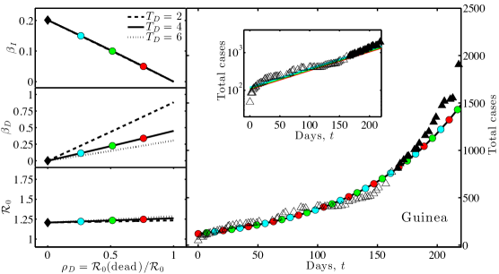
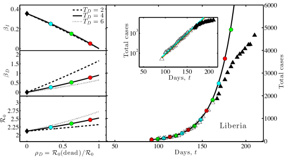
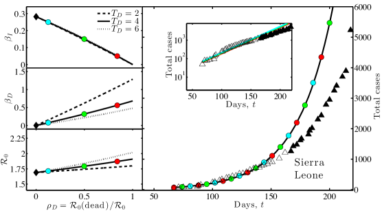
The identifiability problem, described in the previous section, suggests why it is more difficult than has been recognized to ascertain the mechanistic details of EVD transmission from early-stage epidemic data alone. Here, we investigate case data from three countries: Guinea, Liberia and Sierra Leone (data from rivers_github ; see Table 1 for more information). We use an exponential growth curve fit to the cumulative case counts as a target to investigate multiple possible scenarios (Figure 3). For this fit, we extend our SEIRD model to include a more realistic distribution period for the E class eichner2011incubation ; teamebola . The exposed (i.e, latently infected) period is modeled as a gamma distribution with mean of 11 days and 6 classes, so that the standard deviation is 4.5 days (see Supplementary Figure 6). We use the generating-function approach of Wallinga and Lipsitch wallinga2007generation (see Appendix D) to estimate ${\cal{R}}_{0}$ from $\lambda$ while accounting for the chosen time distributions within the E, I and D classes. For each country, the resulting model predictions have two key features (see Figure 3). First, multiple scenarios with varying ratios of transmission risk from living and dead individuals all fit the data equally well. Second, estimates that neglect post-death transmission tend to under-estimate ${\cal{R}}_{0}$. The bottom-left panels of Figure 3 all show an increase in ${\cal{R}}_{0}$ that varies with the fraction of cases caused by post-death transmission, $\rho_{D}$. The increase in ${\cal{R}}_{0}$ due to post-death transmission is of concern. However, there is a tradeoff: larger $\rho_{D}$ means not only a larger ${\cal{R}}_{0}$, but also a larger potential impact of reducing post-death transmission.

Reduction in transmission risk after death can have substantial epidemiological benefits

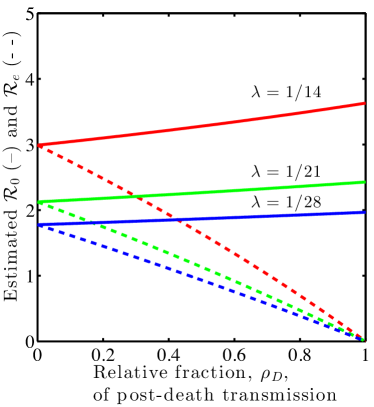
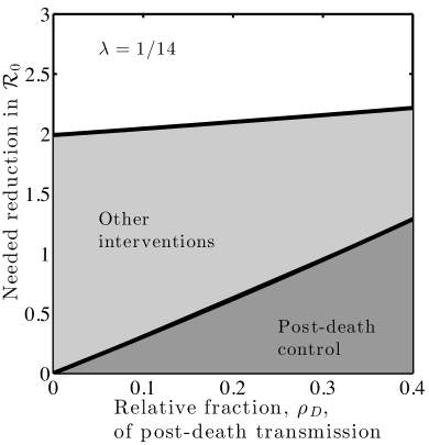
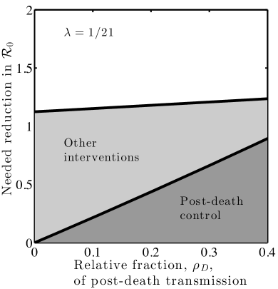
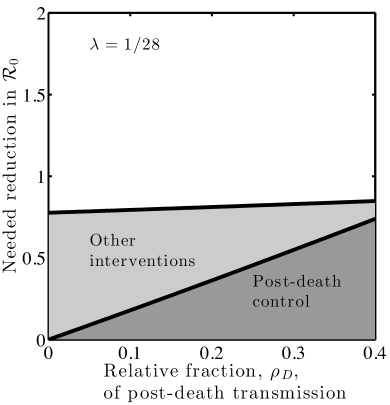
We evaluate the benefits of control in a SEIRD representation of EVD using a gamma distributed E class period. Three scenarios are considered, in which the characteristic epidemic growth times are $1/\lambda=14$, 21 and 28 days and for which we assume $T_{D}=3$ days. Figure 4 summarizes our central findings. We find, as before, that ${\cal{R}}_{0}$ is an increasing function of $\rho_{D}$, the proportion of transmission that occurs post-death. We also find that the inferred basic reproductive number increases with increasing epidemic growth rates. These estimates can be used to evaluate the benefit of control strategies that eliminate (even partially) post-death transmission. In the limit that all post-death transmission is eliminated, the effective reproductive number would be ${\cal{R}}_{e}\equiv(1-\rho_{D}){\cal{R}}_{0}$. In this limit, ${\cal{R}}_{0}$ is reduced by $\rho_{D}{\cal{R}}_{0}$, a substantial amount given estimates of $\rho_{D}$ in the range of 10%-30% teamebola . For example, in the scenarios evaluated, control of post-death transmission reduces ${\cal{R}}_{0}$ by $\approx 0.2-1$ secondary transmission per infected individual. Thus, controlling post-death transmission of EVD could be an important component of epidemic control.

    

    

Figure 4: The effect of controlling post-death transmission of EVD outbreaks with different epidemic growth rates $\lambda$. (Top-left) Basic reproductive numbers, ${\cal{R}}_{0}$, without intervention (solid lines) compared to effective reproductive numbers, ${\cal{R}}_{e}$ by eliminating post-death transmission (dashed lines). Reproductive numbers are plotted against the fraction $\rho_{D}$ of secondary infections due to dead-to-living transmission. For all scenarios, ${\cal{R}}_{e}=(1-\rho_{D}){\cal{R}}_{0}$. (Other panels) Break-down of the needed reduction in ${\cal{R}}_{0}$ to reach a value of ${\cal{R}}_{e}=1$ for each of the characteristic epidemic growth rates examined in the top-left panel. The dark-shaded region denotes the reduction in secondary cases due to elimination of post-death transmission as a function of $\rho_{D}$. The light-shaded region denotes the additional reduction in secondary cases necessary if post-death transmission is eliminated.

Conclusions

The relative importance of post-death transmission is difficult to estimate from epidemic growth rate data alone, and has important implications for estimates of key epidemiological quantities, and for prediction. This difficulty is due to what is classically termed an “identifiability problem” - relevant to EVD and to other emerging or poorly characterized infectious diseases. Despite the challenge in identifying epidemiological parameters, we robustly conclude that neglecting post-death transmission while fitting to epidemic growth rate tends to lead to underestimates of ${\cal{R}}_{0}$. Such underestimates are a potential concern for ongoing efforts to make realistic models of Ebola dynamics and its control.

Here, we have focused on one feature of such control: the use of burial teams and other practices intended to reduce post-death transmission. Burial teams are part of a diverse set of responses required to stop the spread of EVD pandey_2014 . These responses include behavioral changes, hospital interventions meltzer_2014 , and (potentially) vaccination. More burial teams are needed, but recruiting has proven to be difficult due to stigmatization, lack of personal protective equipment, and insufficient compensation of workers reuters_ebola . Previous reports have suggested that some individuals in the population experiencing the epidemic may have acquired immunity to Ebola as a result of sub-clinical infections leroy2000human ; bellan2014ebola . If these individuals exist, and can be identified, they may be valuable contributors to response efforts if they can be recruited as family health-care workers  bellan2014ebola or as part of burial teams. Moving forward, it is essential to consider the logistics of deploying burial teams efficiently and safely while balancing public health benefits and community norms hewlett2003 ; bauch2013 . A better understanding of post-death transmission can help to understand the EVD epidemic in West Africa and plan control efforts, hopefully leading in the long-term to control and elimination of the current outbreak.

Appendix A SEIRD model of Ebola dynamics

The SEIRD model includes the dynamics of susceptible, exposed and infectious individuals, just as in the SEIR model. It differs in that the R class stands for recovered individuals while the D class stands for dead individuals, who are nonetheless infectious. The dynamics can be written as:

$$\frac{{\rm d}S}{{\rm d}t} = -\beta_{I}SI/N-\beta_{D}SD/N$$ (3)

$$\frac{{\rm d}E}{{\rm d}t} = \beta_{I}SI/N+\beta_{D}SD/N-E/T_{E}$$ (4)

$$\frac{{\rm d}I}{{\rm d}t} = E/T_{E}-I/T_{I}$$ (5)

$$\frac{{\rm d}R}{{\rm d}t} = (1-f)I/T_{I}$$ (6)

$$\frac{{\rm d}D}{{\rm d}t} = fI/T_{I}-D/T_{D}$$ (7)

where $\beta_{I}$ is the transmission rate for contacts with infected individuals and $\beta_{D}$ is the transmission rate associated with contacts with dead individuals (who are nonetheless infectious). The other parameters are: $T_{E}$ the average exposed period, $T_{I}$ the average infectious period, $T_{D}$ the average period of infectiousness after death and $f$ the fraction of infected individuals who die. In this model $N=S+E+I+R$. This model neglects birth/immigration of individuals and natural death/emigration. The conventional derivation of the transmission rate is that a susceptible individual interacts with a certain fixed number of individuals per unit time $m$, of which a fraction $I/N$ are infectious, and only a fraction $p$ of which lead to transmission. The transmission rate $\beta_{I}$ is a product of $m$ and $p$. Similarly, here we assume that dead individuals are contacted by a certain fixed number of individuals per unit time $n$, of which a fraction $S/N$ are susceptible, and only a fraction $q$ of contacts lead to transmission. The transmission rate $\beta_{D}$ is a product of $n$ and $q$. The SEIRD model can be extended further to take into account the possibility that the duration of the exposed infectious and dead periods are non-exponential.

Appendix B Estimating the basic reproductive number, ${\cal{R}}_{0}$, for the SEIR and SEIRD models given exponential intra-class period distributions

Infected case data can then be used to estimate unknown epidemiological parameters, including the transmission rate and ${\cal{R}}_{0}$. In the case of the SEIR model, the predicted exponential growth rate, $\lambda$, can be derived from a solution of the linearized dynamics near the value of $(S=N,E=0,I=0,R=0)$. The growth rate $\lambda$ correspond to the largest eigenvalue of the Jacobian:

$$J=\left[\begin{array}[]{c c}-\frac{1}{T_{E}}&\beta_{SEIR}\\ \frac{1}{T_{E}}&-\frac{1}{T_{I}}\end{array}\right]$$ (8)

It can be shown that the growth of the number of infected cases is an exponential of the form $I(t)=I_{0}e^{\lambda t}$ where

$$\lambda=\frac{-(\sigma+\gamma)+\sqrt{\left(\sigma+\gamma\right)^{2}-4\sigma(\gamma-\beta_{SEIR})}}{2}$$ (9)

where $\sigma\equiv 1/T_{E}$ and $\gamma\equiv 1/T_{I}$. The best-fit value of $\beta_{SEIR}$ can be inferred given a measured value $\hat{\lambda}$ and prior estimates for $\sigma$ and $\gamma$. For example,

$${\cal{R}}_{0,SEIR}=(1+\lambda/\sigma)(1+\lambda/\gamma)$$ (10)

where ${\cal{R}}_{0,SEIR}=\beta_{SEIR}/\gamma$, such that

$$\hat{\beta}_{SEIR}=(1+\hat{\lambda}T_{E})(1+\hat{\lambda}T_{I})/T_{I}$$ (11)

Similarly, given the SEIRD model, the predicted exponential growth rate $\lambda$ of the number of infected cases corresponds to the largest eigenvalue of the linearized system near $(N,0,0,0,0)$, of which only the variables $E(t)$, $I(t)$ and $D(t)$ must be tracked. The Jacobian of this subsystem is:

$$J=\left[\begin{array}[]{c c c}-\frac{1}{T_{E}}&\beta_{I}&\beta_{D}\\ \frac{1}{T_{E}}&-\frac{1}{T_{I}}&0\\ 0&\frac{f}{T_{I}}&-\frac{1}{T_{D}}\end{array}\right]$$ (12)

The solutions can be computed exactly.

Appendix C The roots of identifiability problems in estimating the basic reproductive number from early-stage epidemic growth data

Figure 5: Identifiability problem in estimating ${\cal{R}}_{0}$ for a SIR model from exponential epidemic growth data. The synthetic data (black circles) is $I(t)\propto e^{\lambda t}e^{1+\psi}$ where $\lambda=1/28$, corresponding to a characteristic time of 4 weeks and where $\psi$ is a normally distributed random variable with mean 0 and standard deviation 0.1. The model fits correspond to solutions of SIR models in which $\beta=0.107,$ $0.0714$, and $0.0595$ days^-1 and $T_{I}=14$, 28 and 42 days respectively. The basic reproductive number in each case is ${\cal{R}}_{0}=\beta T_{I}$ = 1.5, 2.0 and 2.5 respectively. (Left panel) Each of the SIR model predictions fits the data equally well at early times, despite having very different basic reproductive numbers. (Right panel) The predictions of the long-term dynamics differ, with epidemic size increasing as a function of ${\cal{R}}_{0}$.

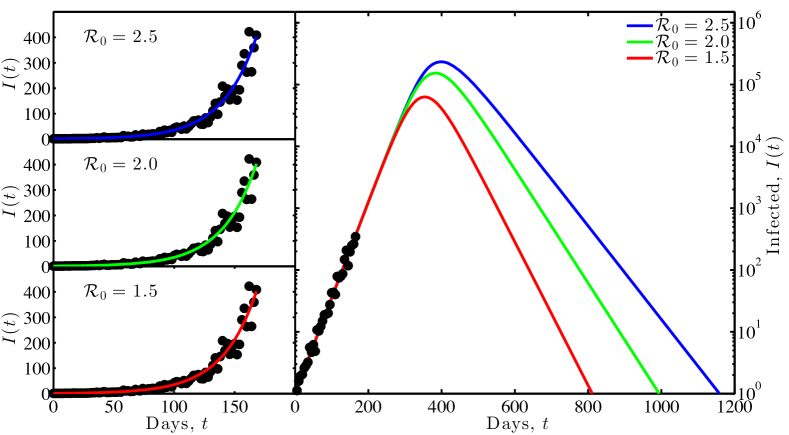
The identifiability problem raised in the main text is a generic issue in epidemiology. By means of illustration, consider the spread of a disease that has no exposed stage, such that it can be suitably described using a SIR model. Further assume that the basic reproductive number of the disease is to be estimated from epidemic case data in which the number of cases is growing at a rate of $\hat{\lambda}=1/28$. The basic reproductive number for a SIR model is $\beta T_{I}$, i.e., the transmission rate multiplied by the infectious period. The epidemic growth rate for a SIR model is $\lambda=\beta-1/T_{I}$, i.e., the difference between the transmission and recovery rate. This can be written as: $\lambda=T_{I}({\cal{R}}_{0}-1)$. Hence, consider three scenarios, in which the true infectious period is $T_{I}=14$, 28 and 42 days. Each of these scenarios is compatible with the same epidemic growth rate $\hat{\lambda}$ given ${\cal{R}}_{0}=1.5$, 2.0 and 2.5. Figure 5 illustrates this point using synthetic data. Note that for a given epidemic growth rate, diseases whose period of infectious is longer have larger basic reproductive numbers. In the example above, a disease with an infectious period of 14 days requires 2 infection cycles (on average) to increase in case count by a factor of e (2.718). Whereas, a disease with an infectious period of 28 days requires 1 infection cycle (on average) to increase in case count by a factor of e (2.718). This is the intuition behind the seemingly paradoxical result that diseases with longer infectious periods are estimated to have higher values of ${\cal{R}}_{0}$ when estimated via the same epidemic growth rate. Moreover, although the disease dynamics may appear indistinguishable at early stages of an epidemic, the long-term dynamics can be quite different. For example, Figure 5 shows how diseases with higher values of ${\cal{R}}_{0}$ infect more people over the long-term despite having the same early time dynamics. Controlling a disease with a higher value of ${\cal{R}}_{0}$ is also more difficult.

Appendix D Estimating the basic reproductive number, ${\cal{R}}_{0}$, for the SEIRD model given arbitrary intra-class period distributions

Wallinga and Lipsitch wallinga2007generation established a formal connection between ${\cal{R}}_{0}$ and the epidemic growth rate, here: $\lambda$, such that

$${\cal{R}}_{0}=\frac{1}{M(-\lambda)}$$ (13)

where

$$M(z)=\int_{0}^{\infty}e^{za}g(a){\rm d}a$$ (14)

The moment generating function $M(z)$ operates on the distribution $g(a)$ which, in epidemiological terms, is the normalized fraction of all secondary cases caused by an infectious individual at “age” $a$ since infection. For example, if individuals are only infectious at a single age $a_{c}$ after infection, then $g(a)=\delta(a-a_{c})$ where $\delta(x)$ is the delta function. Similarly, if individuals recover from being infected at a rate $\gamma$, then $g(a)=\gamma e^{-\gamma a}$, i.e., an exponential distribution. The advantage of this approach is that it is possible to uniquely identify the value of ${\cal{R}}_{0}$ given a measured epidemic growth rate $\hat{\lambda}$ and additional information on the age distributions for secondary infections.

For the SEIRD model, the appropriate generating function is:

$$M(z)=(1-\rho_{D})M_{E}(z)M_{I}(z)+\rho_{D}M_{E}(z)M_{I}(z)M_{D}(z)$$ (15)

where $\rho_{D}$ is the fraction of secondary transmission due to post-death transmission and $1-\rho_{D}$ is the fraction of secondary transmission due to pre-death transmission. We consider a gamma distributed exposed period with $T_{E}=11$ days, and shape parameters $n_{E}=6$ and $b_{E}=n_{E}/T_{E}$ (see Figure 6) whose generating function is:

$$M_{E}(-\lambda)=\left(\frac{b_{E}}{b_{E}+\lambda}\right)^{n_{E}}$$ (16)

We consider here exponentially-distributed periods for the I and D classes. The generating functions are:

$$M_{I}(-\lambda) = \frac{\gamma}{\gamma+\lambda}$$ (17)

$$M_{D}(-\lambda) = \frac{\chi}{\chi+\lambda}$$ (18)

where $\gamma=1/T_{I}$ and $\chi=1/T_{D}$. Therefore for the SEIRD model, it is possible to estimate ${\cal{R}}_{0}$ using the generating function method given observations of an epidemic growth rate and suitable information on epidemiological modes and parameters.

Figure 6: Gamma-distributed exposed period. The distribution has an average exposed period with $T_{E}=11$ days, such that the shape parameters are $n_{E}=6$ and $b_{E}=n_{E}/T_{E}$.

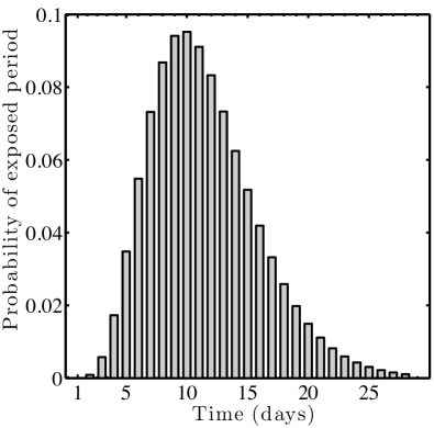
This analysis assumed that the I and D classes are exponentially distributed with characteristic times of 6 and 3 days, respectively. A similar analysis can be performed in which the force of transmission is concentrated with different distributions, e.g., uniform, unimodal or even concentrated at the very end of a fixed epidemic period (so-called delta distributed).

Appendix E Case data information

Cumulative case count data from Guinea, Liberia and Sierra Leone was used as the target of model fits in Figure 3. These data sets were downloaded from Caitlin Rivers’ publicly available github site rivers_github . The time periods over which data is calibrated is shown in Table 1. The start date was selected based on the first day at which the cumulative case count exceeded 50. The final date was set at the end of August, coinciding with reported increases in intervention and widespread dissemination of the severity of the outbreak pandey_2014 . The exponential fits are based on log-transformed cumulative case counts. Additional challenges for inference arise, in part, due to under-reporting meltzer_2014 and lags between incidence and reporting events teamebola .

Country	$T_{0}$	$T_{1}$	$\hat{\lambda}$	Doubling period
Guinea	3/22/14	8/31/14	0.011	61 days
Liberia	6/22/14	8/31/14	0.048	14 days
Sierra Leone	5/28/14	8/31/14	0.032	21 days

Table 1: Data sources for model fits of SEIRD to Ebola epidemic data. The values of $T_{0}$ and $T_{1}$ denote the start and stop dates for the cumulative case data used for estimating the epidemic growth rate, $\hat{\lambda}$. Estimates of the epidemic growth rate were based on linear regression of log-transformed cumulative case counts. The doubling time of the epidemic is defined as $\frac{\log{2}}{\hat{\lambda}}$.

References

- (1) Meltzer, M. I. et al. Estimating the future number of cases in the Ebola epidemic-Liberia and Sierra Leone, 2014–2015. MMWR Surveill Summ 63, 1–14 (2014).
- (2) Lewnard, J. A. et al. Dynamics and control of Ebola virus transmission in Montserrado, Liberia: a mathematical modelling analysis. The Lancet Infectious Diseases (2014).
- (3) Chowell, G., Hengartner, N. W., Castillo-Chavez, C., Fenimore, P. W. & Hyman, J. The basic reproductive number of Ebola and the effects of public health measures: the cases of Congo and Uganda. Journal of Theoretical Biology 229, 119–126 (2004).
- (4) Legrand, J., Grais, R., Boelle, P., Valleron, A. & Flahault, A. Understanding the dynamics of ebola epidemics. Epidemiology and infection 135, 610–621 (2007).
- (5) Francesconi, P. et al. Ebola hemorrhagic fever transmission and risk factors of contacts, uganda. Emerging infectious diseases 9, 1430 (2003).
- (6) Centers for Disease Control and Prevention. Ebola (Ebola Virus Disease) - QAs on Transmission (2014). URL http://www.cdc.gov/vhf/ebola/transmission/qas.html.
- (7) WHO Ebola Response Team. Ebola virus disease in West Africa – the first 9 months of the epidemic and forward projections. New England Journal of Medicine 371, 1481–1495 (2014).
- (8) Lloyd-Smith, J. O., Schreiber, S. J., Kopp, P. E. & Getz, W. Superspreading and the effect of individual variation on disease emergence. Nature 438, 355–359 (2005).
- (9) Galvani, A. P. & May, R. M. Epidemiology: dimensions of superspreading. Nature 438, 293–295 (2005).
- (10) Pandey, A. et al. Strategies for containing Ebola in West Africa. Science 1260612 (2014).
- (11) Gomes, M. F. et al. Assessing the international spreading risk associated with the 2014 West African Ebola outbreak. PLOS Currents Outbreaks (2014).
- (12) Rivers, C. M., Lofgren, E. T., Marathe, M., Eubank, S. & Lewis, B. L. Modeling the Impact of Interventions on an Epidemic of Ebola in Sierra Leone and Liberia. arXiv preprint arXiv:1409.4607 (2014).
- (13) Althaus, C. L. Estimating the reproduction number of Ebola virus (EBOV) during the 2014 outbreak in West Africa. PLOS Currents Outbreaks (2014).
- (14) Ebola Case Data. Maintained by Caitlin Rivers. Accessed: 11/4/2014. URL https://github.com/cmrivers/ebola.
- (15) Chowell, G. & Nishiura, H. Transmission dynamics and control of Ebola virus disease EVD: a review. BMC Medicine 12, 196 (2014).
- (16) Keeling, M. J. & Rohani, P. Modeling Infectious Diseaes in Humans and Animals (Princeton University Press, Princeton, NJ, 2007).
- (17) Wallinga, J. & Lipsitch, M. How generation intervals shape the relationship between growth rates and reproductive numbers. Proceedings of the Royal Society B: Biological Sciences 274, 599–604 (2007).
- (18) Eichner, M., Dowell, S. F. & Firese, N. Incubation period of Ebola hemorrhagic virus subtype Zaire. Osong Public Health and Research Perspectives 2, 3–7 (2011).
- (19) Reuters. Sierra Leone’s burial teams for Ebola victims strike over hazard pay (10/7/2014).
- (20) Leroy, E. et al. Human asymptomatic ebola infection and strong inflammatory response. The Lancet 355, 2210–2215 (2000).
- (21) Bellan, S. E., Pulliam, J. R., Dushoff, J. & Meyers, L. A. Ebola control: effect of asymptomatic infection and acquired immunity. The Lancet 384, 1499–1500 (2014).
- (22) Hewlett, B. S. & Amola, R. P. Cultural contexts of ebola in northern uganda. Emerging infectious diseases 9, 1242 (2003).
- (23) Bauch, C. T. & Galvani, A. P. Social factors in epidemiology. Science 342, 47–49 (2013).