Induced QCD with two auxiliary bosonic fields

Abstract:

Following a proposal of Budczies and Zirnbauer, we investigate an alternative lattice discretization of continuum ${\rm SU}(N_{c})$ Yang-Mills theory in which the self-interactions of the gauge field are induced by a path integral over $N_{b}\geq N_{c}-1$ auxiliary bosonic fields which are coupled linearly to the gauge field. In two dimensions there exists an analytic proof that the new discretization reproduces Yang-Mills theory in its non-perturbative continuum limit. We provide numerical evidence that this is also the case in three and four dimensions and that, after a suitable matching of the free parameters, the results of the induced theory agree with results from the ordinary plaquette action up to lattice artifacts. The new discretization is ideally suited to change the order of integration in the QCD path integral to arrive at formulations in which the gauge fields have been integrated out. The resulting theories might be amenable to methods previously used in the infinite-coupling limit, and we briefly discuss possibilities to arrive at dual representations of lattice QCD.

1 Introduction

Strong-coupling approaches to lattice QCD allow for analytical studies and the construction of new simulation algorithms. Typically, these methods are applicable only if the self-interactions of the gluons are neglected, i.e., in the limit of infinite coupling. There have been several attempts to overcome this problem by “inducing” the gluon dynamics with an action formulated in terms of auxiliary fields [1, 2, 3, 4]. One of the typical problems for these theories of an “induced” version of Yang-Mills theory is that Yang-Mills theory is usually recovered in the limit of an infinite number of auxiliary fields, rendering the application of the methods impractical.

In [5] Budczies and Zirnbauer (BZ) proposed a “designer action” (in their paper for gauge group $G={\rm U}(N_{c})$) conjectured to reproduce continuum Yang-Mills theory when the mass of the auxiliary boson fields approaches a critical value. The major novelty is that this works already for a fixed number of auxiliary fields $N_{b}\geq N_{c}$ for $G={\rm U}(N_{c})$ (or $N_{b}\geq N_{c}-1$ for $G={\rm SU}(N_{c})$, see below). This was shown analytically for $G={\rm U}(N_{c})$ in $d=2$ dimensions by matching to an earlier result of Witten [6]. For $d>2$ there is no analytical proof but a plausible universality argument.

In this proceedings article we investigate the properties of a modified version of the BZ theory for ${\rm SU}(N_{c})$ gauge theory and provide numerical evidence that the continuum limit of the theory equals continuum Yang-Mills theory. The modified version solves a sign problem of the bosonized version of the theory. Here we restrict ourselves to showing only a few numerical and analytical results. More details will be given in a future publication [7]. In section 5 we briefly discuss how this theory can be used to arrive at dual representations of full QCD.

2 Induced Yang-Mills theory

The action introduced by Budzcies and Zirnbauer in [5] is given for a hypercubic lattice by

$$S_{\rm BZ}[\varphi,\bar{\varphi},U]=\sum_{b=1}^{N_{b}}\sum_{\pm\mathbf{p}}\sum_{j=1}^{4}\big{[}m_{\rm BZ}\bar{\varphi}_{b,\mathbf{p}}(x_{j}^{\mathbf{p}})\varphi_{b,\mathbf{p}}(x_{j}^{\mathbf{p}})-\bar{\varphi}_{b,\mathbf{p}}(x_{j+1}^{\mathbf{p}})U(x_{j+1}^{\mathbf{p}},x_{j}^{\mathbf{p}})\varphi_{b,\mathbf{p}}(x_{j}^{\mathbf{p}})\big{]}\,,$$ (1)

where $U\in G$ are the link variables, $\varphi$ are auxiliary bosonic fields, $b$ labels the number of boson flavors, and $m_{\rm BZ}$ is a mass parameter (which we take to be real) satisfying $m_{\rm BZ}>1$. The index $\mathbf{p}$ labels oriented plaquettes, and $j$ labels the points of the plaquette in order of the orientation. Integration over the auxiliary fields in the path integral yields the weight factor

$$\omega_{\rm BZ}[U]=\int[d\varphi]\exp\big{\{}-S_{\rm BZ}[\varphi,\bar{\varphi},U]\big{\}}=\prod_{p}\big{|}\det\big{(}m_{\rm BZ}^{4}-U_{p}\big{)}\big{|}^{-2N_{b}}\,,$$ (2)

where the product is over all unoriented plaquettes $p$, i.e., every plaquette is counted only once, and $U_{p}$ is the usual product of $U$-fields around the plaquette. We rewrite this factor in terms of the coupling $\alpha_{\rm BZ}=m_{\rm BZ}^{-4}$ as

$$\omega_{\rm BZ}[U]\sim\prod_{p}\big{|}\det\big{(}1-\alpha_{\rm BZ}\,U_{p}\big{)}\big{|}^{-2N_{b}}\,.$$ (3)

As shown in [5] for $G={\rm U}(N_{c})$, this theory has a continuum limit for a fixed number of bosonic fields $N_{b}$ when $\alpha_{\rm BZ}\to 1$ as long as $N_{b}\geq N_{c}$. This can be shown by investigating the behavior of the weight factor for a particular plaquette $U_{p}$ in this limit. The continuum limit is obtained when the weight factor approaches the $\delta$-function, i.e., for any analytic function $f:G\to\mathbbm{C}$

$$\lim_{\alpha_{\rm BZ}\to 1}\frac{\langle f\rangle}{\langle 1\rangle}=f(\mathbbm{1})\,,\quad\langle f\rangle=\int_{G}dU_{p}\,f(U_{p})\big{|}\det\big{(}1-\alpha_{\rm BZ}U_{p}\big{)}\big{|}^{-2N_{b}}\,.$$ (4)

Furthermore, for the special case of $d=2$ the continuum limit reproduces the boundary partition function of Wittens combinatorial treatment of Yang-Mills theory [6]. For $d>2$ there is no strict proof, but it was argued in [5] that in higher dimensions the collectivity of the gauge fields is increased, which works in favor of “universality”. Thus, if Yang-Mills theory is induced in $d=2$, it should also be induced in $d>2$.

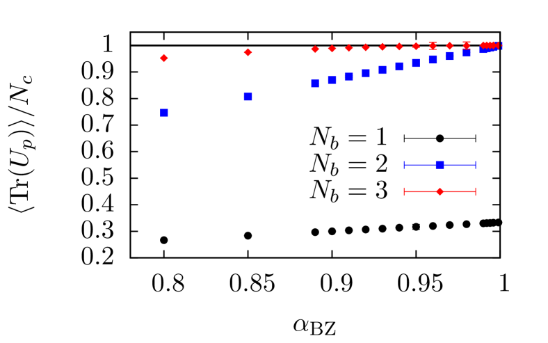
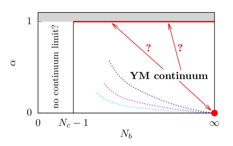
Figure 1: Left: Expectation value (4) of the test function $f(U_{p})={\rm Tr}(U_{p})/N_{c}$ for $G={\rm SU}(3)$ in the approach to the limit $\alpha_{\rm BZ}=1$. Right: Conjectured phase diagram in the $(N_{b},\alpha)$-plane for $G={\rm SU}(N_{c})$. The dashed lines indicate possible lines of constant physics.

The extension of the existence proof of a continuum limit from $G={\rm U}(N_{c})$ to $G={\rm SU}(N_{c})$ is not completely straightforward. The exception is the ${\rm SU}(2)$ case for which a proof with $N_{b}=1$ was already given in [5]. We will discuss the details of the proof for $G={\rm SU}(N_{c})$ in our future publication [7]. Instead of considering the integral analytically one can also investigate the behavior of the one-link integral (4) for certain test functions numerically in the limit $\alpha_{\rm BZ}\to 1$. The results for $G={\rm SU}(3)$ and $f(U_{p})={\rm Tr}(U_{p})/N_{c}$ for different values of $N_{b}$ are shown in figure 1 (left). The plot indicates that the integral indeed approaches $f(\mathbbm{1})=1$ once we have reached the critical number of boson fields, which appears to be $N_{b}=N_{c}-1$ for ${\rm SU}(N_{c})$ in contrast to $N_{b}=N_{c}$ for ${\rm U}(N_{c})$. Other test functions show the same behavior. This implies that for $G={\rm SU}(N_{c})$ the continuum limit exists for $\alpha_{\rm BZ}\to 1$ if $N_{b}\geq N_{c}-1$. This is consistent with our analytical findings.

3 Sign problem and modified theory

While the weight factor (3) is positive definite, this is not the case for the exponential of the action (1) considered in [5], which is complex for a general configuration of auxiliary bosonic fields. In future applications, e.g., simulations of the bosonized version, this would be problematic. Fortunately, the sign problem can be eliminated by a simple reformulation of the theory. The corresponding weight factor is given by

$$\omega[U]=\prod_{p}\Big{[}\det\big{(}1-\frac{\alpha}{2}\big{(}U_{p}+U_{p}^{\dagger}\big{)}\big{)}\Big{]}^{-N_{b}}\,,$$ (5)

where $\alpha$ is related to $\alpha_{\rm BZ}$. The equivalence of the two weight factors up to an unimportant constant is evident when the absolute value in (3) is written out explicitly. The corresponding action with auxiliary bosonic fields is given by

$$\begin{array}[]{rcl}\displaystyle S_{B}[\varphi,\bar{\varphi},U]&=\displaystyle\sum_{b=1}^{N_{b}}\sum_{p}\sum_{j=1}^{4}\Big{[}&m\bar{\varphi}_{b,p}(x^{p}_{j})\varphi_{b,p}(x^{p}_{j})-\bar{\varphi}_{b,p}(x^{p}_{j+1})U(x^{p}_{j+1},x^{p}_{j})\varphi_{b,p}(x^{p}_{j})\Big{.}\vspace*{2mm}\\ &&\displaystyle\Big{.}-\bar{\varphi}_{b,p}(x^{p}_{j})U(x^{p}_{j},x^{p}_{j+1})\varphi_{b,p}(x^{p}_{j+1})\Big{]}\end{array}$$ (6)

with $2/\alpha=m^{4}-4m^{2}+2$ and $x_{j}^{p}=x_{j}^{+\mathbf{p}}$. Note that $\alpha_{\rm BZ}\to 1$ is equivalent to $\alpha\to 1$. In figure 1 (right) we show the conjectured phase diagram in the $(N_{b},\alpha)$-plane for $G={\rm SU}(N_{c})$.

4 Numerical investigation of the continuum limit

We now investigate the properties of the limit $\alpha\to 1$ in the numerically cheap case of three-dimensional ${\rm SU}(2)$ gauge theory via simulations with the weight factor (5). We fix $N_{b}$ to 1 and 2 to see whether both cases lead to the correct continuum limit. To make contact with Yang-Mills theory we compare the simulation results to results obtained with the standard Wilson plaquette action. The simulations for the induced theory are done using local Metropolis updates and links that evolve randomly in an $\epsilon$-ball around the old ones. For the Wilson action we use the standard mixture of heatbath and overrelaxation updates. In pure gauge theory the only quantity that has to be fixed to render the simulations predictive is the lattice spacing $a$, here determined via the Sommer scale $r_{0}$ [8]. If both theories approach the same continuum theory, one expects that below some critical lattice spacing both theories give the same results up to lattice artifacts.

We observe that for the whole range of couplings $\beta$ typically considered in simulations of ${\rm SU}(2)$ gauge theory at $d=3$ (see, e.g., [9]) there exists a matching coupling $\alpha$ with the same value of $r_{0}/a$. Using this as a matching condition, we obtain a matching relation of the form

$$\beta(\alpha)=\frac{b_{-1}}{1-\alpha}+b_{0}+b_{1}(1-\alpha)+\ldots\,.$$ (7)

This relation is valid for the range of lattice spacings used in our simulations and all values of $N_{b}\geq N_{c}-1$ with $N_{b}$-dependent coefficients $b_{n}$. In particular, the expected divergence at $\alpha=1$ behaves like $1/(1-\alpha)$ to very good accuracy.

Using this matching and tuning the couplings to the ones from [10] we have performed high-precision simulations in the induced theory for the static $q\bar{q}$-potential via Polyakov loop correlators evaluated with the multilevel algorithm [11]. We have then reproduced the analysis of [10] and extracted the boundary coefficient $\bar{b}_{2}$ [12] appearing in the effective string theory for the QCD flux tube (for a review see, e.g., [13]). Note that our focus here is on a like-by-like comparison and not on validating the string picture. The quantity $\bar{b}_{2}$ is ideal in this respect since it probes the subleading properties of the potential and, presumably, is non-universal. The details of the analysis, the computations, and a full list of references will be given in [7]. The results for $\bar{b}_{2}$ are shown in figure 2 (left) for different values of $r_{0}$ in comparison to the results of [10, 14]. The plot indicates good agreement of the results with the ones obtained with the Wilson action. Furthermore, the results are significantly different from the ones obtained in ${\rm SU}(3)$ and $Z_{2}$ gauge theory [15], leading to the conclusion that the continuum potential indeed corresponds to that of ${\rm SU}(2)$ Yang-Mills theory.

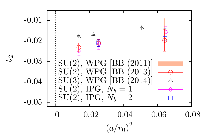
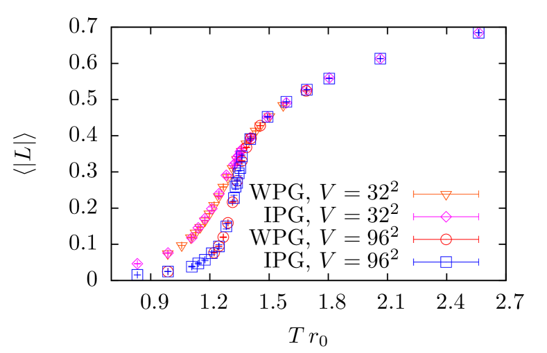
Figure 2: Left: Comparison of results from the induced (IPG) and the Wilson (WPG) action [10, 14] for $\bar{b}_{2}$ vs. $a^{2}$. Right: Results for the absolute value of the Polyakov loop on the two extremal volumes at $N_{t}=4$.

We have also investigated the finite-temperature transition for $N_{t}=4$ with volumes between $V/a^{2}=32^{2}$ and $96^{2}$. The Polyakov loop on the two extremal volumes with $N_{b}=2$ is shown in figure 2 (right). The plot shows very good agreement between the two sets of points. Performing an extraction of critical exponents following [16] we obtain $T_{c}r_{0}=1.34(2)$ and $\gamma/\nu=1.69(4)$ in good agreement with the corresponding Wilson results. To confirm this agreement we will increase the statistics at $T_{c}$ and repeat the analysis for $N_{t}=6$. Results for $N_{b}=1$ will be shown in [7].

5 Dual representations of QCD

A very interesting feature of the induced theory is that it allows us to change the order of integration in the QCD path integral, i.e., to integrate over the gauge fields first. The part of the action (6) containing the link $U_{\mu}(x)$ (here we have switched to the standard notation where $x$ is a particular point on the lattice) can be written as

$$S_{B;x,\mu}^{\text{hop}}(\varphi,\bar{\varphi},U)=-\frac{1}{2}{\rm Tr}\left[A_{\mu}(x,\varphi,\bar{\varphi})U+A^{\dagger}_{\mu}(x,\varphi,\bar{\varphi})U^{\dagger}\right]\,,$$ (8)

where $A_{\mu}$ is a complex matrix constructed from the auxiliary fields. Since the weight for a given link does not depend on other link variables the path integral over the gluonic degrees of freedom factorizes into a product over integrals of the type

$$\mathcal{I}_{\mu}(x,\varphi,\bar{\varphi})=\int_{G}dU\,e^{\frac{1}{2}{\rm Tr}[A_{\mu}(x,\varphi,\bar{\varphi})U+A^{\dagger}_{\mu}(x,\varphi,\bar{\varphi})U^{\dagger}]}\,.$$ (9)

The exact solution of this integral is known for $G=U(N_{c})$ [17] and for some $N_{c}$ also for $G={\rm SU}(N_{c})$ [18, 19, 20]. In our future publication [7] we will derive a general solution for $G={\rm SU}(N_{c})$,

$$\mathcal{I}=2^{N_{c}(N_{c}-1)/2}\biggl{(}\prod_{n=1}^{N_{c}-1}n!\biggr{)}\sum_{\nu=0}^{\infty}\varepsilon_{\nu}\cos\big{(}\nu\theta\big{)}\frac{\det\big{[}\lambda_{i}^{j-1}I_{\nu+j-1}\big{(}\lambda_{i}\big{)}\big{]}}{\Delta\big{(}\lambda^{2}\big{)}}\,,$$ (10)

where we have suppressed the dependence on $\mu,x,\varphi$, and $\bar{\varphi}$ for simplicity. $\varepsilon_{\nu}$ is Neumann’s factor ($\varepsilon_{\nu=0}=1$ and $\varepsilon_{\nu>0}=2$), $\exp(i\theta)$ is the complex phase of $\det(A)$, the $\lambda_{i}^{2}$ are the $N_{c}$ eigenvalues of $AA^{\dagger}$, $\Delta$ is the Vandermonde determinant, and $I$ denotes modified Bessel functions of the first kind.

Using this result the dual partition function of the induced theory is given by

$$Z=\int[d\varphi]\,\exp\Big{\{}-\sum_{b=1}^{N_{b}}\sum_{p}\sum_{j=1}^{4}m\bar{\varphi}_{b,p}(x^{p}_{j})\varphi_{b,p}(x^{p}_{j})\Big{\}}\prod_{x,\mu}\mathcal{I}_{\mu}(x,\varphi,\bar{\varphi})\,.$$ (11)

Another dual partition function with a similar structure has been obtained for the Wilson action using Hubbard-Stratonovich transformations [21].

Full QCD also includes dynamical fermions. Those can be added to the induced theory in the standard way using the lattice discretization of choice. The partition function for full QCD is then

$$Z=\int[dU]\,[d\varphi]\,[d\psi][d\bar{\psi}]\exp\big{\{}-S_{F}[\psi,\bar{\psi},U]-S_{B}[\varphi,\bar{\varphi},U]\big{\}}\,.$$ (12)

Using staggered-type fermions, possibly at nonzero chemical potential, the fermion action is

$$S_{F}=\sum_{x}\Big{\{}\sum_{\mu}\left[\bar{\psi}(x)\rho_{\mu}(x)\,U_{\mu}(x)\psi(x+\hat{\mu})+\bar{\psi}(x+\hat{\mu})\tilde{\rho}_{\mu}(x)\,U^{\dagger}_{\mu}(x)\psi(x)\right]+m_{q}\bar{\psi}(x)\psi(x)\Big{\}}\,,$$ (13)

where the factors $\rho$ and $\tilde{\rho}$ include the usual staggered phases and factors originating from the introduction of the chemical potential. There are several options how to proceede to derive dual representations of QCD. One possibility is to expand the exponential over Grassmann fields as

$$e^{-S_{F}}=\prod_{x}\Big{\{}\Big{[}\prod_{a}\sum_{n_{a}(x)}\big{(}M_{a}(x)\big{)}^{n_{a}(x)}\Big{]}\prod_{\mu}\prod_{a,b}\Big{[}\sum_{p_{ab}(x,\mu)}\big{(}H_{ab,\mu}(x)\big{)}^{p_{ab}(x,\mu)}\sum_{\tilde{p}_{ab}(x,\mu)}\big{(}\widetilde{H}_{ab,\mu}(x)\big{)}^{\tilde{p}_{ab}(x,\mu)}\Big{]}\Big{\}}$$ (14)

with $\>\>M_{a}(x)=-m_{q}\;\bar{\psi}_{a}(x)\psi_{a}(x)$, $\>\>H_{ab,\mu}(x)=-\rho_{\mu}(x)\,[U_{\mu}(x)]_{ab}\,\bar{\psi}_{a}(x)\psi_{b}(x+\hat{\mu})\>\>$ and $\>\>\widetilde{H}_{ab,\mu}(x)=\\ -\tilde{\rho}_{\mu}(x)\,[U^{\dagger}_{\mu}(x)]_{ba}\,\bar{\psi}_{b}(x+\hat{\mu})\psi_{a}(x)$. Here, $n_{a}(x)$, $p_{ab}(x,\mu)$, and $\tilde{p}_{ab}(x,\mu)$ are the dual variables, which are either $0$ or $1$, and $a$ and $b$ are color indices. The QCD partition function is then rewritten in terms of a partition sum over the dual variables. Performing the Grassmann integrals yields constraints of the form

$$n_{a}(x)+\sum_{\mu,b}\big{[}\tilde{p}_{ba}(x-\hat{\mu},\mu)+p_{ab}(x,\mu)\big{]}=n_{a}(x)+\sum_{\mu,b}\big{[}p_{ba}(x-\hat{\mu},\mu)+\tilde{p}_{ab}(x,\mu)\big{]}=1\,.$$ (15)

In the final step one can perform the integrals over the gluonic degrees of freedom, which is possible because they appear linearly in the exponent. Note that link variables also appear in front of the exponential due to the terms in (14). They can be expressed as derivatives of the integral (9).

This procedure is not optimal in the sense that gauge invariance is not manifest because the constraints (15) are incomplete. Using only (15) one would generate many configurations whose contribution to gauge-invariant quantities is zero after averaging over gauge fields. We are currently deriving additional constraints on the dual variables to ensure that we sample only configurations whose contribution is nonzero after averaging. This will lead to a partition function with similar constituents as the partition function previously obtained in the infinite-coupling limit, see, e.g., [22] and references therein, except that we will have additional loops with contributions from the auxiliary bosonic fields. The resulting partition function will probably have a sign problem and therefore needs further treatment to make numerical simulations possible.

6 Conclusions

We have presented a study of the continuum limit of a theory that is conjectured to provide an alternative discretization of Yang-Mills theory. Numerical results show good agreement with simulations using the usual Wilson action, for quantities at both zero and nonzero temperature, already at finite lattice spacings in the approach to the continuum limit. This provides evidence that the continuum limit indeed corresponds to Yang-Mills theory. The new theory, when formulated in terms of auxiliary bosonic fields, can be used to derive dual presentations of QCD by methods previously only applicable in the infinite-coupling limit. Further details will be given in our future publication [7].

- [1] M. Bander, Phys.Lett. B126 (1983) 463.
- [2] H. W. Hamber, Phys.Lett. B126 (1983) 471.
- [3] V. Kazakov and A. A. Migdal, Nucl.Phys. B397 (1993) 214 [hep-th/9206015].
- [4] A. Hasenfratz and P. Hasenfratz, Phys.Lett. B297 (1992) 166 [hep-lat/9207017].
- [5] J. Budczies and M. Zirnbauer, math-ph/0305058.
- [6] E. Witten, Commun.Math.Phys. 141 (1991) 153.
- [7] B. B. Brandt, R. Lohmayer, and T. Wettig, in preparation.
- [8] R. Sommer, Nucl.Phys. B411 (1994) 839 [hep-lat/9310022].
- [9] B. B. Brandt and P. Majumdar, Phys.Lett. B682 (2009) 253 [arXiv:0905.4195].
- [10] B. B. Brandt, PoS EPS-HEP2013 (2013) 540 [arXiv:1308.4993].
- [11] M. Luscher and P. Weisz, JHEP 0109 (2001) 010 [hep-lat/0108014].
- [12] O. Aharony and N. Klinghoffer, JHEP 1012 (2010) 058 [arXiv:1008.2648].
- [13] B. Lucini and M. Panero, Phys.Rept. 526 (2013) 93 [arXiv:1210.4997].
- [14] B. B. Brandt, JHEP 1102 (2011) 040 [arXiv:1010.3625].
- [15] M. Billo et al., JHEP 1205 (2012) 130 [arXiv:1202.1984].
- [16] J. Engels et al., Nucl.Phys.Proc.Suppl. 53 (1997) 420 [hep-lat/9608099].
- [17] R. C. Brower, P. Rossi, and C.-I. Tan, Phys.Rev. D23 (1981) 942.
- [18] M. Creutz, J.Math.Phys. 19 (1978) 2043.
- [19] R. C. Brower and M. Nauenberg, Nucl.Phys. B180 (1981) 221.
- [20] K. Eriksson, N. Svartholm, and B. Skagerstam, J.Math.Phys. 22 (1981) 2276.
- [21] H. Vairinhos and P. de Forcrand, arXiv:1409.8442.
- [22] P. de Forcrand, J. Langelage, O. Philipsen, and W. Unger, Phys.Rev.Lett. 113 (2014) 152002 [arXiv:1406.4397].