Abstract

We study the physics of probe D6-branes with quantized internal worldvolume flux in the ABJM background with unquenched massless flavors. This flux breaks parity in the (2+1)-dimensional gauge theory and allows quantum Hall states. Parity breaking is also explicitly demonstrated via the helicity dependence of the meson spectrum. We obtain general expressions for the conductivities, both in the gapped Minkowski embeddings and in the compressible black hole ones. These conductivities depend on the flux and contain a contribution from the dynamical flavors which can be regarded as an effect of intrinsic disorder due to quantum fluctuations of the fundamentals. We present an explicit, analytic family of supersymmetric solutions with nonzero charge density, electric, and magnetic fields.

1 Introduction and motivation

The quantum Hall effect (QHE) is a fascinating phenomenon in gapped (2+1)-dimensional systems with broken parity symmetry. When electrons are confined in a heterojunction at low temperature and strong magnetic fields, the response to an applied electric field displays a striking behavior: the conductivity in the direction of the electric field vanishes, while the transverse conductivity is quantized and given by $(e^{2}/h)\nu$, where $\nu$ is the filling fraction, defined as the ratio of the charge density to the magnetic flux. In the integer quantum Hall effect (IQHE) $\nu\in{\mathbb{Z}}$, whereas $\nu$ is a rational number in the fractional quantum Hall effect (FQHE).

Since its discovery more than thirty years ago, the QHE has been the subject of intense research. Nevertheless, some aspects of the FQHE involve strongly-coupled dynamics and are still not fully understood. The holographic AdS/CFT duality has proven to be a powerful tool in the study of quantum matter in the strongly-coupled regime, since it provides answers to difficult field theory questions by using classical gravitational theories in higher dimensions. Therefore, it is quite natural to explore the possibility of constructing holographic models of the (F)QHE and to extract properties that are very difficult to obtain via weakly-coupled many-body field theory.

In recent years, two types of holographic models of the QHE have been proposed. The first class consists of bottom-up models in Einstein-Maxwell-axio-dilaton theories [1, 2, 3, 4, 5]. These models are endowed with an $SL(2,{\mathbb{Z}})$ duality and, as a consequence, they capture some observed features of QH physics. However, it is very difficult to engineer these types of models to have a mass gap; [6] is so far the only example of a gapped model in this class.

The second approach to holographically realize the QHE makes use of top-down D-brane constructions [7, 8, 9], in which a (2+1)-dimensional gauge theory with fermions in the fundamental representation is modeled by a suitable D$p$-D$q$ brane intersection. The limit in which the D$q$-brane is treated as a probe in the D$p$-brane background corresponds in the field theory dual to the so-called quenched approximation in which loops of fundamental fermions are neglected. In this approach, the worldvolume theory of the probe brane encodes the physics of the fermions. Generically, the probe brane crosses the horizon, yielding a black hole embedding, which is dual to a gapless metallic state. The quantum Hall state is realized holographically as a Minkowski embedding, in which the brane ends smoothly above the black hole horizon. The distance from the horizon at which the probe caps off determines the mass gap.

In this paper we will follow the top-down probe-brane approach and construct quantum Hall states in the ABJM theory with unquenched massless flavors. The unflavored ABJM model is a $U(N)\times U(N)$ Chern-Simons gauge theory in 2+1 dimensions with levels $(k,-k)$ and bifundamental matter fields [10]. In string theory, the ABJM theory is realized as the low-energy limit of multiple M2-branes at a ${\mathbb{C}}^{4}/{\mathbb{Z}}_{k}$ singularity. When $N$ and $k$ are large, this theory admits a supergravity description, preserving 24 supersymmetries, in terms of a $AdS_{4}\times{\mathbb{C}}{\mathbb{P}}^{3}$ geometry with fluxes in type IIA ten-dimensional supergravity. Due to its high degree of supersymmetry, the ABJM theory is one of the models where the AdS/CFT correspondence has been tested with great precision. Since the boundary theory is conformally invariant and the bulk metric therefore has an $AdS$ factor, the gauge/gravity dictionary is firmly established.

The ABJM model can be generalized by adding flavors, i.e., fields transforming in the fundamental representations $(N,1)$ and $(1,N)$ of the $U(N)\times U(N)$ gauge group, which we will refer to as “quarks” in analogy with the terminology of holographic QCD. In the holographic setup, these flavors are due to D6-branes extended in $AdS_{4}$ and wrapping an ${\mathbb{R}}{\mathbb{P}}^{3}$ cycle inside ${\mathbb{C}}{\mathbb{P}}^{3}$ [11, 12]. This configuration preserves ${\cal N}=3$ supersymmetry. The quenched approximation of these holographic quarks, where the D6-branes are treated as probes, has been studied in [13, 14, 15, 17, 16].

However, it is possible to go beyond the quenched approximation and include the backreaction of the D6-branes; there are simple analytic geometries which encode the dynamics of the flavors in the Veneziano limit[18]. Here we will employ the solution found in [19, 20] by smearing the D6-branes. This smearing technique is applicable when the number $N_{f}$ of flavor branes is large and can be continuously distributed in the internal space, which changes the flavor group from $U(N_{f})$ to $U(1)^{N_{f}}$. For massless flavors the result is simply a metric which differs from the unflavored one merely by constant squashing factors. The construction was generalized in [22] to the backreaction of massive flavors. These squashing factors depend on $N_{f}$ and encode the effects of dynamical flavor loops.

In this paper, we want to engineer quantum Hall states in the flavored ABJM theory. Such Hall states are only possible if parity is broken, which can be accomplished by turning on an appropriate internal flux on the D6-brane worldvolume. However, treating the backreaction of this internal flux is quite challenging. For now, we will start with a single quenched massive quark in the background of $N_{f}$ unquenched massless quarks, a system analyzed in [23, 20]. We then will turn on a parity-breaking internal flux on the worldvolume of this probe D6-brane.

In the presence of this internal flux, the Wess-Zumino term of the probe action contains the term $\int\hat{C}_{1}\wedge F^{3}$, where $\hat{C}_{1}$ is the pullback of the RR potential one-form. In the ABJM background $C_{1}$ has only internal components. Therefore, after integrating over the internal directions, we are left with an axionic term $F\wedge F$ along $AdS_{4}$, which indeed breaks parity and corresponds to a Chern-Simons term on the boundary.

Even in the probe limit, choosing a consistent ansatz for this internal flux, which must also be quantized appropriately, is not obvious. We can, however, take a cue from the ABJ model [24], i.e., the $U(N+M)_{k}\times U(N)_{-k}$ Chern-Simons matter theory, which can be engineered in string theory by adding fractional D2-branes to the ABJM setup. The corresponding gravity dual can be obtained from the ABJM solution by turning on a flat Neveu-Schwarz $B_{2}$ field proportional to the Kähler form of ${\mathbb{C}}{\mathbb{P}}^{3}$. The pullback of this parity-breaking $B_{2}$ on a probe D6-brane can alternately be viewed as a worldvolume gauge field flux. Inspired by this example, we will generalize this ABJ solution into an ansatz for the case with no background $B_{2}$ field and only a probe worldvolume flux, but with backreacted massless flavors.

Equipped with this ansatz for the internal gauge flux, we will show that, indeed, there are quantum Hall states in this setup. From the QH perspective, one can regard the effects of the massless, backreacted quarks as representing intrinsic disorder due to the quantum fluctuations of the massive quark. We will compute the contribution of these fluctuations to the conductivities in the form of an integral extended in the holographic direction, from the tip of the brane to the $AdS$ boundary.

Surprisingly, we will find a very special family of explicit, supersymmetric, gapped QH solutions at zero temperature. These BPS solutions have nonzero charge density and equal electric and magnetic fields, and we can compute the Hall conductivity, including the effects of quark loops, analytically.

The rest of this paper is organized as follows. In Section 2 we review the ABJM background with flavor. Then, in Section 3, we consider the embedding of a probe D6-brane with internal flux. We first present in Section 3.1 the ansatz for the internal components of the worldvolume gauge field that will be used throughout the paper and discuss the corresponding flux quantization condition. In Section 3.2 we generalize these results to nonvanishing background electric and magnetic fields, as well as to nonzero charge density and currents. We compute the corresponding longitudinal and transverse conductivities in Section 4.

In Section 5 we analyze the residual $SO_{+}(1,1)$ boost invariance of our system at zero temperature. An analytic supersymmetric solution of the equations of motion at zero temperature is presented in Section 6. Section 7 is devoted to the analysis of quark-antiquark bound states, i.e., mesons. In particular, we study the effect of the broken parity on the mass spectrum. In Section 8 we summarize our results and discuss possible future directions.

The paper is completed with several appendices. In Appendix A we provide details of our background geometry and discuss the quantization condition of the worldvolume flux obtained by comparison with the ABJ solution. Appendix B contains a detailed analysis of the equations of motion of the probe. The kappa symmetry of the embeddings is analyzed in Appendix C. Finally, the equations governing the fluctuations of the probe are the subject of Appendix D, where we also estimate the meson masses using a WKB approximation.

2 The ABJM background with flavor

In this section we will review, following [19, 25, 23, 20], the background geometry corresponding to the ABJM model with unquenched massless flavors in the smeared approximation. Additional details of this supergravity solution are given in Appendix A. The ten-dimensional metric, in string frame, has the form

$$ds^{2}\,=\,L^{2}\,\,ds^{2}_{BH_{4}}\,+\,ds^{2}_{6}\,\,,$$ (2.1)

where $L$ is the radius of curvature, $ds^{2}_{BH_{4}}$ is the metric of a planar black hole in the four-dimensional Anti-de Sitter space, given by

$$ds^{2}_{BH_{4}}=-r^{2}h(r)dt^{2}+\frac{dr^{2}}{r^{2}h(r)}+r^{2}\big{[}dx^{2}+dy^{2}\big{]}\ ,$$ (2.2)

and $ds^{2}_{6}$ is the metric of the compact internal six-dimensional manifold. The blackening factor $h(r)$ is given by

$$h(r)\,=\,1\,-\,\frac{r_{h}^{3}}{r^{3}}\ ,$$ (2.3)

where the horizon radius $r_{h}$ is related to the temperature $T$ by $T={3\,r_{h}\over 4\pi}$. The internal metric $ds^{2}_{6}$ in (2.1) is a deformation of the Fubini-Study metric of ${\mathbb{C}}{\mathbb{P}}^{3}$, realized as an ${\mathbb{S}}^{2}$-bundle over ${\mathbb{S}}^{4}$. Let $ds^{2}_{{\mathbb{S}}^{4}}$ be the standard metric for the unit round four-sphere and let $z^{i}$ ($i=1,2,3$) be three Cartesian coordinates parameterizing the unit two-sphere ($\sum_{i}(z^{i})^{2}\,=\,1$). Then, $ds^{2}_{6}$ can be written as:

$$ds^{2}_{6}\,=\,{L^{2}\over b^{2}}\,\,\Big{[}\,q\,ds^{2}_{{\mathbb{S}}^{4}}\,+\,\big{(}dz^{i}\,+\,\epsilon^{ijk}\,A^{j}\,z^{k}\,\big{)}^{2}\,\Big{]}\ ,$$ (2.4)

where $A^{i}$ are the components of the non-Abelian one-form connection corresponding to an $SU(2)$ instanton. In Appendix A we give a more explicit representation of the $ds^{2}_{6}$ line element in terms of alternative coordinates.

The parameters $b$ and $q$ in (2.4) are constant squashing factors which encode the effect of the massless flavors in the backreacted metric. Indeed, when $q=b=1$ the metric (2.4) is just the canonical Fubini-Study metric of the ${\mathbb{C}}{\mathbb{P}}^{3}$ manifold with radius $2L$ in the so-called twistor representation. In this case (2.1) is the metric of the unflavored ABJM model at nonzero temperature. When the effect of the delocalized D6-brane sources is taken into account, the resulting metric is deformed as in (2.4). It was shown in [19] that at zero temperature the particular deformation written in (2.4) preserves ${\cal N}=1$ SUSY.

The parameter $b$ in (2.4) represents the relative squashing of the ${\mathbb{C}}{\mathbb{P}}^{3}$ part of the metric with respect to the $AdS_{4}$ part due to the flavor, while $q$ parameterizes an internal deformation which preserves the ${\mathbb{S}}^{4}$-${\mathbb{S}}^{2}$ split of the twistor representation of ${\mathbb{C}}{\mathbb{P}}^{3}$. The explicit expressions for the coefficients $q$ and $b$ found in [19] are given below. They depend on the number of colors $N$ and flavors $N_{f}$, as well as on the ’t Hooft coupling $\lambda\,=\,N/k$, through the combination

$$\hat{\epsilon}\,\equiv\,{3N_{f}\over 4k}\,=\,{3\over 4}\,\,{N_{f}\over N}\,\lambda\ ,$$ (2.5)

where the factor $3/4$ is introduced for convenience. It is also useful to define the quantity $\eta$ as:

$$\eta\,=\,1\,+\,{3N_{f}\over 4k}\,=\,1+\hat{\epsilon}\ ,\qquad\qquad\eta\in[1,\infty)\ .$$ (2.6)

In terms of the deformation parameter $\hat{\epsilon}$, the squashing factors $q$ and $b$ are:

$$q = 3+\frac{3}{2}\hat{\epsilon}-2\sqrt{1+\hat{\epsilon}+\frac{9}{16}\hat{\epsilon}^{2}}\ ,$$

$$b = \frac{2q}{q+1}\ .$$ (2.7)

As functions of $\hat{\epsilon}$, the squashing parameters $q$ and $b$ are monotonically increasing functions, which approach the values $q\approx 5/3$ and $b\approx 5/4$ as $\hat{\epsilon}\to\infty$. Another way to encode the loop effects of the massless sea quarks is to define the screening factor $\sigma$:

$$\sigma\,=\,\sqrt{{(4-3b)(2-b)b^{3}\over 2(b-1)\eta+b}}\ .$$ (2.8)

Without flavors, $\sigma=1$, and as $\hat{\epsilon}\to\infty$, $\sigma\to 0$. The $AdS$ radius $L$ can then expressed in terms of $\lambda$ and the screening factor:

$$L^{2}\,=\,\pi\sqrt{2\lambda}\,\sigma\ .$$ (2.9)

The complete solution of type IIA supergravity with sources is endowed with RR two- and four-forms $F_{2}$ and $F_{4}$, as well as with a constant dilaton $\phi$ (whose value depends on $N$, $N_{f}$, and $k$). Their explicit expressions are given in the Appendix A.

It is worth mentioning at this point that the background summarized in this section has been generalized in [22] to the case in which the quarks are massive (at zero temperature). As we increase the mass of the quarks, these generalized solutions interpolate between the geometry reviewed above (for zero quark mass) and the unflavored ABJM background (for infinitely massive quarks).

3 D6-brane probes with flux

We are interested in dynamics of a massive quark holographically dual to a probe D6-brane with internal flux in the flavored ABJM background. The D6-brane extends along $r$ and the three Minkowski directions and, wraps on the internal manifold a three-cycle topologically equivalent to ${\mathbb{R}}{\mathbb{P}}^{3}={\mathbb{S}}^{3}/{\mathbb{Z}}_{2}$. This three-cycle will be parameterized by three angles $\alpha$, $\beta$, and $\psi$, and will be characterized by an embedding function $\theta(r)$. With this embedding, the D6-brane then has an induced metric given by (for details see Appendix A):

$${ds^{2}_{7}\over L^{2}} = r^{2}\,\left[-h(r)\,dt^{2}+dx^{2}+dy^{2}\right]+{1\over r^{2}}\,\left({1\over h(r)}+{r^{2}\,\theta^{\prime\,2}\over b^{2}}\,\right)\,dr^{2}$$ (3.1)

$$\qquad+\,{1\over b^{2}}\,\Big{[}q\,d\alpha^{2}+q\,\sin^{2}\alpha\,d\beta^{2}+\sin^{2}\,\theta\,\left(\,d\psi\,+\,\cos\alpha\,d\beta\,\right)^{2}\,\Big{]}\ ,$$

where $0\leq\alpha<\pi$, $0\leq\beta,\psi<2\pi$, and $\theta=\theta(r)$ determines the profile of the probe brane. Notice that the second line in (3.1) is the line element of a squashed ${\mathbb{R}}{\mathbb{P}}^{3}$.

For a supersymmetric configuration at zero temperature, it is possible to use kappa symmetry to find an explicit solution for $\theta(r)$ (see the analysis in [19] and in Appendix C). But, in general we will have to numerically solve the equations of motion to find $\theta(r)$.

The thermodynamic properties of D6-branes embedded in this way were studied in detail in [20]. Here we will generalize some of these results by including worldvolume gauge fields. In particular, we will turn on a nontrivial flux on the internal cycle. In the rest of this section we will determine the form of this internal worldvolume flux which gives rise to a consistent solution of the brane equations of motion.

3.1 Internal flux

Since we are primarily interested in gapped, QH states, let us focus on Minkowski (MN) embeddings of the probe, in which the brane ends smoothly at a radial position $r_{*}$ above the horizon, i.e., $r_{*}>r_{h}$. The D6-brane can cap off smoothly if, at the tip of the brane $r=r_{*}$, the angle $\theta$ reaches its minimal value $\theta=0$ where an ${\mathbb{S}}^{1}\subset{\mathbb{R}}{\mathbb{P}}^{3}$ shrinks to zero. At the tip, the last term of (3.1) vanishes and the induced metric takes the form:

$${ds^{2}_{7}\over L^{2}}\Big{|}_{r=r_{*}}=r^{2}\,\big{[}-h_{*}dt^{2}+dx^{2}+dy^{2}\big{]}+{q\over b^{2}}\,\,\Big{[}d\alpha^{2}\,+\,\sin^{2}\alpha\ d\beta^{2}\Big{]}\ ,$$ (3.2)

where $h_{*}=h(r=r_{*})$. From (3.2), we see that at the tip of the brane the coordinates $\alpha$ and $\beta$ span a non-collapsing ${\mathbb{S}}^{2}_{*}$. As in other probe-brane QH models [7, 8], we want to turn on a flux of the worldvolume gauge field $F$ on this non-shrinking sphere.

Of course, this flux must be quantized appropriately. We will adopt the following quantization condition:

$${1\over 2\pi\alpha^{\prime}}\,\int_{{\mathbb{S}}^{2}_{*}}\,F\,=\,{2\pi M\over k}\ ,\qquad\qquad M\in{\mathbb{Z}}\,\,.$$ (3.3)

Notice that, compared with the ordinary flux quantization condition of the worldvolume gauge field, we are considering in (3.3) $M/k$ fractional units of flux. In Appendix A we verify that (3.3) is the correct prescription for the flux quantization by studying the background without massless flavors, i.e., $N_{f}=0$. In this case one can induce an internal $F$ flux through ${\mathbb{S}}^{2}_{*}$ by switching on a flat Neveu-Schwarz $B_{2}$ field proportional to the Kähler form of ${\mathbb{C}}{\mathbb{P}}^{3}$. Then, the quantization condition (3.3) follows from the fractional holonomy of $B_{2}$ along the ${\mathbb{C}}{\mathbb{P}}^{1}$ cycle of ${\mathbb{C}}{\mathbb{P}}^{3}$. In this setup the integer $M$ is the number of fractional D2-branes and this configuration is dual to the ABJ model [24] with gauge group $U(N+M)_{k}\times U(N)_{-k}$. We also check in Appendix A that $M$ can be identified with the Page charge for fractional D2-branes.

Let us now write a concrete ansatz for the internal gauge field $F$. We will represent $F$ in terms of a potential one-form $A$ given by:

$$A\,=\,L^{2}\,a(r)\,(d\psi+\cos\alpha\,d\beta)\ ,$$ (3.4)

where the $L^{2}$ factor is introduced for convenience and $a=a(r)$ is a function of the radial coordinate which determines the varying flux on the $(\alpha,\beta)$ two-sphere. The field strength $F=dA$ corresponding to (3.4) is simply:

$$F\,=\,L^{2}\Big{[}a^{\prime}(r)\,dr\wedge(d\psi+\cos\alpha d\beta)\,-\,a(r)\,\sin\alpha\,d\alpha\wedge d\beta\Big{]}\ ,$$ (3.5)

which restricted to ${\mathbb{S}}^{2}_{*}$ becomes:

$$F\big{|}_{{\mathbb{S}}^{2}_{*}}\,=\,-L^{2}\,a_{*}\,\sin\alpha\,d\alpha\wedge d\beta\ ,$$ (3.6)

where $a_{*}\equiv a(r=r_{*})$ is the value of the flux function at the tip. It follows that

$$\int_{{\mathbb{S}}^{2}_{*}}\,F\,=\,-4\pi\,L^{2}\,a_{*}\ ,$$ (3.7)

and the condition (3.3) quantizes the values of $a_{*}$ in the following way:

$$a_{*}\,=\,-{\pi M\over kL^{2}}\,\,,\qquad\qquad M\in{\mathbb{Z}}\ .$$ (3.8)

Let us denote the value of the flux function at the tip as:

$$a_{*}\,=\,-Q\ .$$ (3.9)

To write the quantization condition (3.8) in terms of physical quantities, recall that the $AdS$ radius $L$ can be written as in (2.9). Plugging this into (3.8), we find the following quantization condition for $Q$:

$$Q\,=\,{\sqrt{\lambda}\over\sqrt{2}\,\sigma}\,{M\over N}\ ,\qquad\qquad M\in{\mathbb{Z}}\ .$$ (3.10)

Using the ansatz (3.5) for the internal flux, we can try to find a solution for a MN embedding of the probe D6-brane. In Appendix B we check that (3.5), together with embedding ansatz corresponding to the induced metric (3.1), is a consistent truncation of the equations of motion of the probe.

At zero temperature, we have found an analytic solution for $\theta(r)$ and the flux function $a=a(r)$ which preserves two of the four supercharges of the ${\cal N}=1$ superconformal background. The explicit calculations are performed in Appendix C with the use of kappa symmetry. Here we just quote the result for $\theta(r)$ and $a(r)$:

$$\cos\theta(r) = \Big{(}{r_{*}\over r}\Big{)}^{b}$$ (3.11)

$$a(r) = -Q\,(\cos\theta(r))^{{1\over q}}\,=\,-Q\,\Big{(}{r_{*}\over r}\Big{)}^{{b\over q}}\ .$$ (3.12)

However, to realize the quantum Hall states we are interested in, we need to generalize our ansatz for the gauge field to include electric and magnetic fields, as well as the components dual to the charge density and current. We analyze this more general set up in the next subsection.

3.2 Background fields and currents

If we want a more general ansatz that includes background electric and magnetic fields and the associated charged current, we need to consider other components of the worldvolume gauge field. In the standard way, a magnetic field $B$ and an electric field $E$ are added by turning on the radial zero modes of $F_{xy}$ and $F_{0x}$. The charge density is holographically related to $F_{r0}$, the longitudinal and Hall currents come from $F_{rx}$ and $F_{ry}$. We therefore take the worldvolume gauge field to have the form:

$$A\,=\,L^{2}\,\Big{[}\,a_{0}(r)\,dt\,+(Et+\,a_{x}(r))\,dx\,+\,(B\,x+a_{y}(r))\,dy\,+\,a(r)\,(d\psi+\cos\alpha\,d\beta)\,\Big{]}\ .$$ (3.13)

We can continue to use the induced metric ansatz given by (3.1), characterized by the embedding function $\theta=\theta(r)$.

Interestingly, due to our choice in (3.13) of the internal components of the gauge field, the dependence of the action on the internal angles of the ${\mathbb{R}}{\mathbb{P}}^{3}$ cycle factorizes and consequently, we can consistently take the functions $\theta$, $a$, $a_{0}$, $a_{x}$, and $a_{y}$ to depend only on the radial variable. After integrating over the internal angles $\alpha$, $\beta$, and $\psi$, the DBI action of the D6-brane for our ansatz can be written as:

$$S_{DBI}\,=\int d^{3}x\,dt\,{\cal L}_{DBI}\ ,$$ (3.14)

where the DBI Lagrangian density ${\cal L}_{DBI}$ can be compactly written as:

$${\cal L}_{DBI}\,=\,-{8\pi^{2}\,L^{7}\,T_{D6}\,e^{-\phi}\over b^{4}}\,{\sqrt{(B^{2}+r^{4})h-E^{2}}\,\sqrt{q^{2}+b^{4}\,a^{2}}\over\sqrt{h}}\,\sqrt{\Delta}\ ,$$ (3.15)

where $T_{D6}$ is the D6-brane tension and the quantity $\Delta$ is defined to be

$$\Delta = b^{4}r^{2}ha^{\prime\,2}\,+\,\sin^{2}\theta\,\Bigg{[}b^{2}+r^{2}h\,\theta^{\prime\,2}\,$$ (3.16)

$$\qquad\qquad\qquad+{b^{2}h\over E^{2}-(B^{2}+r^{4})h}\,\Big{[}(Ba_{0}^{\prime}+Ea_{y}^{\prime})^{2}\,+\,r^{4}(a_{0}^{\prime\,2}-ha_{x}^{\prime\,2}+ha_{y}^{\prime\,2})\Big{]}\Bigg{]}\,\,.\qquad\qquad$$

The Wess-Zumino term of the action is:

$$S_{WZ}\,=\,T_{D6}\int_{{\cal M}_{7}}\,\left(\hat{C}_{7}\,+\,\hat{C}_{5}\wedge F\,+\,{1\over 2}\,\hat{C}_{3}\wedge F\wedge F\,+\,{1\over 6}\hat{C}_{1}\wedge F\wedge F\wedge F\right)\ ,$$ (3.17)

where, $\hat{C}_{7}$, $\hat{C}_{5}$, $\hat{C}_{3}$, and $\hat{C}_{1}$ are the pullbacks to the D6-brane of the RR gauge fields. All of these terms, except for $\hat{C}_{5}\wedge F$, give non-vanishing contributions to the equations of motion.

In the holographic setup, the charge density is encoded in the bulk by the radial electric displacement field $\tilde{D}(r)$, which is given by the derivative of the DBI Lagrangian density with respect to the radial component of the physical electric field. From the ansatz (3.13), and taking into account the physical gauge field $A_{phys}=A/(2\pi\alpha^{\prime})$, we find:

$$\tilde{D}\,=\,{\partial{\cal L}_{DBI}\over\partial A_{0,phys}^{\prime}}\,=\,{2\pi\alpha^{\prime}\over L^{2}}\,{\partial{\cal L}_{DBI}\over\partial a_{0}^{\prime}}\ .$$ (3.18)

We will set $\alpha^{\prime}=1$ from now on. In order to write $\tilde{D}(r)$ in a compact fashion, let us define a function $g(r)$ as:

$$g(r)\,=\,{q+\eta\over 2b(2-q)}\,{r^{4}\,h^{{3\over 2}}\,\sin^{2}\theta\,\sqrt{q^{2}+b^{4}\,a^{2}}\over\sqrt{(B^{2}+r^{4})\,h\,-E^{2}}\,\sqrt{\Delta}}\ .$$ (3.19)

Then, one can show that:

$$\tilde{D}(r)\,=\,{N\sigma^{2}\over 4\pi}\,\tilde{d}(r)\ ,$$ (3.20)

where $\sigma$ is the screening factor defined in (2.8) and $\tilde{d}(r)$ is the function:

$$\tilde{d}(r)\,\equiv\,{g\over h}\,\left[\left(1+{B^{2}\over r^{4}}\right)\,a_{0}^{\prime}\,+\,{BE\over r^{4}}\,a_{y}^{\prime}\,\right]\,\,.$$ (3.21)

The total charge density is obtained by taking the boundary value of $\tilde{D}(r)$, which is proportional to:

$$d\,=\,\lim_{r\to\infty}\,\tilde{d}(r)\ .$$ (3.22)

Similarly, the physical currents along the $x$ and $y$ directions are given by:

$$J_{x}\,=\,{2\pi\alpha^{\prime}\over L^{2}}\,{\partial{\cal L}_{DBI}\over\partial a_{x}^{\prime}}\ ,\qquad\qquad\tilde{J}_{y}\,=\,{2\pi\alpha^{\prime}\over L^{2}}\,{\partial{\cal L}_{DBI}\over\partial a_{y}^{\prime}}\ .$$ (3.23)

One can readily prove that:

$$J_{x}\,=\,{N\sigma^{2}\over 4\pi}\,j_{x}\,\,,\qquad\qquad\qquad\tilde{J}_{y}\,=\,{N\sigma^{2}\over 4\pi}\,\tilde{j}_{y}\ ,$$ (3.24)

where $j_{x}$ turns out to be:

$$j_{x}\,=\,-g\,a_{x}^{\prime}\ ,$$ (3.25)

and $\tilde{j}_{y}(r)$ is:

$$\tilde{j}_{y}(r)\,\equiv\,g\,\left[-\left(1-{E^{2}\over r^{4}h}\right)\,a_{y}^{\prime}\,+\,{BE\over r^{4}h}\,a_{0}^{\prime}\,\right]\ .$$ (3.26)

The equations of motion for the probe are worked out in detail in Appendix B. In particular, $J_{x}$ is constant in $r$ (see (B.29)) and represents the longitudinal current parallel to the electric field. On the other hand, $\tilde{J}_{y}(r)$ depends on the holographic variable. The transverse current $J_{y}$ is obtained as the value of $\tilde{J}_{y}(r)$ at the UV boundary $r\to\infty$ which, according to (3.23), is determined from the limit:

$$j_{y}\,=\,\lim_{r\to\infty}\,\tilde{j}_{y}(r)\ .$$ (3.27)

The radial dependence of $\tilde{d}$ and $\tilde{j}_{y}$ is determined by the $a_{0}$ and $a_{y}$ equations of motion, (B.28) and (B.30). With the definitions introduced above, they can be simply written as:

$$\partial_{r}\,\tilde{d} = B(\eta\,\cos\theta\,a^{\prime}-a\,\sin\theta\,\theta^{\prime})$$ (3.28)

$$\partial_{r}\,\tilde{j}_{y} = E(\eta\,\cos\theta\,a^{\prime}-a\,\sin\theta\,\theta^{\prime})\,\,.$$ (3.29)

In the unflavored case $\eta=1$, these two equations (3.28) and (3.29) can be integrated once because their right-hand side is proportional to $\partial_{r}(a\cos\theta)$. Indeed, for the unflavored background $a_{0}(r)$ and $a_{y}(r)$ are cyclic and can be eliminated by performing the appropriate Legendre transformation.

This is not the case, however, when $\eta\not=1$. We can formally integrate (3.28) and (3.29), defining the integral $I(r)$ as:

$$I(r) \equiv \,\int_{r}^{\infty}\,\Big{(}\eta\,\cos\theta(\bar{r})\,a^{\prime}(\bar{r})\,-\,a(\bar{r})\,\sin\theta(\bar{r})\,\theta^{\prime}(\bar{r})\Big{)}\,d\bar{r}$$ (3.30)

$$= \,-\cos\theta(r)\,a(r)\,+\,(\eta-1)\,\int_{r}^{\infty}\cos\theta(\bar{r})\,a^{\prime}(\bar{r})\,d\bar{r}\ ,$$ (3.31)

where we have integrated by parts to obtain the second line. Clearly,

$$\lim_{r\to\infty}\,I(r)\,=\,0\ ,$$ (3.32)

and equations (3.28) and (3.29) can be written as

$$\tilde{d}(r)\,=\,d\,-\,B\,I(r)\ ,\qquad\qquad\tilde{j}_{y}(r)\,=\,j_{y}\,-\,E\,I(r)\ .$$ (3.33)

Since $a_{0}$ and $a_{y}$ are no longer cyclic, we need a new strategy to solve the equations of motion. Interestingly, there is still one conserved quantity associated with the equations of motion for $A_{0}$ and $A_{y}$. Eq. (B.33) can be recast as the radial independence of the quantity:

$$\Pi\,\equiv\,E\,\tilde{d}(r)\,-\,B\,\tilde{j}_{y}(r)\ .$$ (3.34)

Indeed, the equation $\partial_{r}\,\Pi=0$ follows immediately from (3.28) and (3.29). This implies that $\Pi$ can be written in terms of quantities evaluated at the boundary:

$$\Pi\,=\,E\,d\,-\,B\,j_{y}\ .$$ (3.35)

One can now try to write $a_{0}^{\prime}$, $a_{y}^{\prime}$, and $a_{x}^{\prime}$ in terms of the embedding function $\theta(r)$ and the flux function $a(r)$. Let us work this out in detail. First, we notice that one can invert Eqs. (3.21) and (3.26) and write $a_{0}^{\prime}$ and $a_{y}^{\prime}$ in terms of $\tilde{d}$ and $\tilde{j}_{y}$:

$$a_{0}^{\prime}\,=\,{h\Big{(}1-{E^{2}\over r^{4}\,h}\Big{)}\,\tilde{d}\,+\,{EB\over r^{4}}\,\tilde{j}_{y}\over g\Big{(}1+{B^{2}\over r^{4}}\,-\,{E^{2}\over r^{4}\,h}\Big{)}}\ ,\qquad\qquad a_{y}^{\prime}\,=\,{{EB\over r^{4}}\,\tilde{d}\,-\,\Big{(}1+{B^{2}\over r^{4}}\Big{)}\,\tilde{j}_{y}\over g\Big{(}1+{B^{2}\over r^{4}}\,-\,{E^{2}\over r^{4}\,h}\Big{)}}\ .$$ (3.36)

Notice that (3.36) are not actually solutions for $a_{0}^{\prime}$ and $a_{y}^{\prime}$ since $g$ on the right-hand side is written in terms of these same fields. However, one can write an expression of $g$ in terms of $\theta$ and $a$. Let us define $X$ as:

$$X\equiv h\left(1+{B^{2}\over r^{4}}\,-\,{E^{2}\over r^{4}\,h}\right)\Bigg{[}\left({q+\eta\over 2b^{2}(2-q)}\right)^{2}r^{4}h(q^{2}+b^{4}\,a^{2})\,\sin^{2}\theta+h\tilde{d}^{\,2}-j_{x}^{2}-\tilde{j}_{y}^{\,2}\Bigg{]}-\,{\left(hB\tilde{d}-E\tilde{j}_{y}\right)^{2}\over r^{4}}\ .$$ (3.37)

Then, after some calculation, we obtain:

$$g\,=\,{\sin\theta\,\sqrt{X}\over\Big{(}1+{B^{2}\over r^{4}}\,-\,{E^{2}\over r^{4}\,h}\Big{)}\,\sqrt{b^{2}\,r^{2}\,h\,a^{\prime\,2}\,+\,\sin^{2}\theta\,(1+{r^{2}\over b^{2}}\,h\,\theta^{\prime\,2})}}\,\,.$$ (3.38)

Therefore, we have for $a_{0}^{\prime}$, $a_{x}^{\prime}$, and $a_{y}^{\prime}$:

$$a_{0}^{\prime}\,=\,{\sqrt{b^{2}\,r^{2}\,h\,a^{\prime\,2}\,+\,\sin^{2}\theta\,(1+{r^{2}\over b^{2}}\,h\,\theta^{\prime\,2})}\over\sin\theta\sqrt{X}}\,\Bigg{[}h\left(1-{E^{2}\over r^{4}\,h}\right)\,\tilde{d}\,+\,{EB\over r^{4}}\,\tilde{j}_{y}\Bigg{]}\,\,,$$

$$a_{x}^{\prime}\,=\,-{\sqrt{b^{2}\,r^{2}\,h\,a^{\prime\,2}\,+\,\sin^{2}\theta\,(1+{r^{2}\over b^{2}}\,h\,\theta^{\prime\,2})}\over\sin\theta\sqrt{X}}\,\left(1+{B^{2}\over r^{4}}\,-\,{E^{2}\over r^{4}\,h}\right)\,j_{x}\,\,,$$

$$a_{y}^{\prime}\,=\,{\sqrt{b^{2}\,r^{2}\,h\,a^{\prime\,2}\,+\,\sin^{2}\theta\,(1+{r^{2}\over b^{2}}\,h\,\theta^{\prime\,2})}\over\sin\theta\sqrt{X}}\,\Bigg{[}{EB\over r^{4}}\,\tilde{d}\,-\,\left(1+{B^{2}\over r^{4}}\right)\,\tilde{j}_{y}\Bigg{]}\,\,.$$ (3.39)

The right-hand sides of (3.39) contain the radial functions $\tilde{d}$ and $\tilde{j}_{y}$, which in turn can be written as in (3.33) in terms of the constants $d$ and $j_{y}$, and the integral $I(r)$ defined in (3.30).

In principle, we could use (3.39) to eliminate $a_{0}^{\prime}$, $a_{x}^{\prime}$, and $a_{y}^{\prime}$ from the equations of motion and to reduce the system to an effective problem for the functions $\theta(r)$ and $a(r)$. However, when $\eta\not=1$, the functions $\tilde{d}(r)$ and $\tilde{j}_{y}$ depend non-locally on $\theta(r)$ and $a(r)$ and the corresponding reduced equations of motion would be a system of integro-differential equations for $\theta(r)$ and $a(r)$, which does not seem to be very easy to solve in practice. In the case in which there are no flavors backreacting on the geometry, i.e., when $\eta=q=b=1$, the integral $I(r)$ is just $I=-\cos\theta\,a$ and we can write $\tilde{d}$ and $\tilde{j}_{y}$ simply as $\tilde{d}\,=\,d\,+\,B\cos\theta\,a$ and $\tilde{j}_{y}\,=\,j_{y}+E\cos\theta\,a$. Thus, in this quenched case one can eliminate the gauge fields $a_{0}$, $a_{x}$, and $a_{y}$ and reduce the problem to a system of two coupled, second-order differential equations for $\theta(r)$ and $a(r)$.

3.3 Minkowski embeddings

Having obtained the equations of motion for the D6-brane probe, the next step is to try to solve them. Although, as we will discuss in Section 6, there are special analytic BPS solutions, in general we will have to resort to numerics.

Probe brane solutions are categorized into two classes by their IR behavior. The generic solution is a black hole embedding, in which the brane falls into the horizon; these correspond holographically to gapless, compressible states. In certain special circumstances, the brane can end smoothly at some $r=r_{*}$ when a wrapped cycle shrinks to zero size; these are Minkowski (MN) embeddings. MN solutions with broken parity correspond to gapped, quantum Hall states.

As discussed above in Section 3.1, for a D6-brane probe in the flavored ABJM background, MN embeddings occur when $\theta(r_{*})=0$ for some $r_{*}$. In order to have a physical, finite-energy solution, the embedding $\theta(r)$ and the worldvolume gauge field $F$ must be regular at the tip; that is, the induced metric (3.1) must be smooth, and $a^{\prime}$, $a_{0}^{\prime}$, $a_{x}^{\prime}$, $a_{y}^{\prime}$ must all be finite. Given that the function $g$ (3.38) vanishes at the tip of the brane, the regularity of $a_{0}^{\prime}$ and $a_{y}^{\prime}$ at the tip, combined with (3.21) and (3.26), implies that

$$\tilde{d}(r_{*})\,=\,j_{x}\,=\,\tilde{j}_{y}(r_{*})\,=\,0\,\,.$$ (3.40)

We can interpret this condition to mean that there are no sources at the tip, which is physically sensible as the D6-brane could not support such a source. Suppose that $\tilde{d}(r_{*})\not=0$; this radial displacement field would have to be sourced, for example, by fundamental strings stretching from the horizon. Due to the shrinking cycle, the effective radial tension of the D6-brane vanishes at the tip, so these strings would then pull the D6-brane into the horizon, resulting in a black hole embedding.

The filling fraction $\nu$ is defined by

$$\nu\,=\,2\pi\,\frac{D_{phys}}{B_{phys}}\ ,$$ (3.41)

where the physical magnetic field $B_{phys}$ is related to $B$ by

$$B_{phys}\,=\,{L^{2}\over 2\pi}\,B\,=\,\sqrt{{\lambda\over 2}}\,\sigma\,B\ .$$ (3.42)

Combining (3.40) with (3.33) gives $d=BI(r_{*})$, and the filling fraction for MN solutions is therefore

$$\nu\,=\,{N\sigma\over\sqrt{2\lambda}}\,\frac{d}{B}\,=\,{N\sigma\over\sqrt{2\lambda}}\,I(r_{*})\ ,$$ (3.43)

or, more explicitly using (3.31),

$$\nu\,=\,{M\over 2}\,\left[1\,+\,(\eta-1)\,\int_{r_{*}}^{\infty}\,\cos\theta(r)\,{a^{\prime}(r)\over Q}\,dr\,\right]\ ,$$ (3.44)

where $M$ is the quantization integer and $Q$ is minus the flow function at the tip (see (3.9)). Note that, (3.44) shows explicitly that, for a QH state with nonzero charge density, a nonzero flux is required. Moreover, $\nu$ is the sum of two contributions. The first term in (3.44) is proportional to the flux at the tip. The second term is only nonzero in the unquenched case $\eta\not=1$ and contains an integral from the tip to the boundary. In terms of $N_{f}$ and $k$, $\nu$ takes the form:

$$\nu\,=\,{M\over 2}\,\left[1\,+\,{3N_{f}\over 4k}\,\int_{r_{*}}^{\infty}\,\cos\theta(r)\,{a^{\prime}(r)\over Q}\,dr\,\right]\ .$$ (3.45)

It follows that $\nu$ is a half-integer in the quenched case but gets corrections due to the massless sea quark loops in the unquenched Veneziano limit.

Numerically integrating the equations of motion, we have verified that there are MN solutions obeying the tip regularity conditions (3.40). At this point, we will be content with evidence for MN solutions with nonzero charge density $d$ and magnetic field $B$. We will defer a more thorough study of the possible MN solutions to the future.

4 Conductivities

We are interested in analyzing the longitudinal and transverse conductivity of our configurations. In order to relate these quantities with the variables we have employed, let us point out that the physical electric field $E_{phys}$ is related to the quantity $E$ used above as:

$$E_{phys}\,=\,{L^{2}\over 2\pi}\,E\,=\,\sqrt{{\lambda\over 2}}\,\sigma\,E\ .$$ (4.1)

The longitudinal and transverse conductivities $\sigma_{xx}$ and $\sigma_{xy}$ are defined in terms of $J_{x}$, $J_{y}\equiv\tilde{J}_{y}(r\to\infty)$ and $E_{phys}$ as:

$$\sigma_{xx}\,=\,{J_{x}\over E_{phys}}\ ,\qquad\qquad\sigma_{xy}\,=\,{J_{y}\over E_{phys}}\ .$$ (4.2)

The conductivities can be written as

$$\sigma_{xx}\,=\,{N\sigma\over 2\pi\sqrt{2\lambda}}\,{j_{x}\over E}\ ,\qquad\qquad\sigma_{xy}\,=\,{N\sigma\over 2\pi\sqrt{2\lambda}}\,{j_{y}\over E}\ .$$ (4.3)

In the next two subsections we obtain formulas for $\sigma_{xx}$ and $\sigma_{xy}$ for the two types of embeddings (Minkowski and black hole) of the D6-brane probe.

4.1 Quantum Hall states

Let us now suppose that we have a Minkowski (MN) embedding. To compute the conductivities, we will adapt the method of [7, 8] but with some new twists. In particular, we use the invariance of $\Pi$ under the the holographic flow. The conductivity comes directly from the condition (3.40) that there are no charge sources at the tip $r=r_{*}$. Since $j_{x}$ in (3.25) must be equal to zero,

$$\sigma_{xx}\,=\,0\ .$$ (4.4)

Furthermore, (3.40) implies that $\Pi$ vanishes at $r=r_{*}$ and, since it is radially invariant, $\Pi=0$ at all values of $r$. From (3.35), we see that this is equivalent to $E\,d=B\,j_{y}$; the Hall conductivity is then:

$$\sigma_{xy}\,=\,{N\sigma\over 2\pi\sqrt{2\lambda}}\,{j_{y}\over E}\,=\,{N\sigma\over 2\pi\sqrt{2\lambda}}\,{d\over B}\ .$$ (4.5)

From (3.43), we find that

$$\sigma_{xy}\,=\,{\nu\over 2\pi}\ ,$$ (4.6)

which is exactly what one would expect for a QH state.

4.2 Gapless states

Let us now consider black hole embeddings, in which the D6-brane crosses the horizon at $r=r_{h}$. These embeddings correspond to gapless states. To compute the conductivity, we employ the pseudohorizon argument of [26] to Eq. (3.39). Let $r=r_{p}$ be the position of the pseudohorizon, which is determined by the conditions:

$$h_{p}\,(r_{p}^{4}+B^{2}) = E^{2}$$

$$j_{x}^{2}\,+\,\tilde{j}_{y}^{2}(r_{p}) = \left({q+\eta\over 2b^{2}(2-q)}\right)^{2}\,h_{p}\,r_{p}^{4}\,\sin^{2}\theta_{p}\,\left(q^{2}+b^{4}\,a_{p}^{2}\right)\,+\,h_{p}\,\tilde{d}(r_{p})^{2}$$

$$E\,\tilde{j}_{y}(r_{p}) = B\,h_{p}\,\tilde{d}(r_{p})\ ,$$ (4.7)

where $h_{p}\equiv h(r_{p})$, $\theta_{p}\equiv\theta(r_{p})$, and $a_{p}\equiv a(r_{p})$. It follows that the currents in $x$- and $y$-directions are given by:

$$j_{x} = \sqrt{h_{p}}\,\Bigg{[}\left(1-{B^{2}h_{p}\over E^{2}}\right)\,\tilde{d}^{\,2}(r_{p})\,+\,\left({q+\eta\over 2b^{2}(2-q)}\right)^{2}\,r_{p}^{4}\,(q^{2}+b^{4}\,a_{p}^{2})\,\sin^{2}\theta_{p}\Bigg{]}^{{1\over 2}}$$

$$j_{y} = {B\,h_{p}\over E}\,d\,+\,E\,\left[1-{B^{2}h_{p}\over E^{2}}\right]\,I(r_{p})\ .$$ (4.8)

Notice that the previous expression involves the value of the integral $I$ extended between the $r_{p}$ and the boundary. Therefore, the conductivities are:

$$\sigma_{xx} = {N\sigma\over 2\pi\sqrt{2\lambda}}\,{\sqrt{h_{p}}\over E}\,\Bigg{[}\left(1-{B^{2}h_{p}\over E^{2}}\right)\,\tilde{d}^{\,2}(r_{p})\,+\,\left({q+\eta\over 2b^{2}(2-q)}\right)^{2}\,r_{p}^{4}\,(q^{2}+b^{4}\,a_{p}^{2})\,\sin^{2}\theta_{p}\Bigg{]}^{{1\over 2}}$$

$$\sigma_{xy} = {N\sigma\over 2\pi\sqrt{2\lambda}}\,\Bigg{[}{B\,h_{p}\over E^{2}}\,d\,+\,\left[1-{B^{2}h_{p}\over E^{2}}\right]\,I(r_{p})\Bigg{]}\ .$$ (4.9)

For small electric field, $r_{p}$ is close to the horizon radius $r_{h}$. At first order in $E^{2}$ we can estimate $r_{p}$ as:

$$r_{p}\,\approx\,r_{h}\,\left(1\,+\,{E^{2}\over 3(r_{h}^{4}+B^{2})}\right)\ .$$ (4.10)

With this result we can write $h_{p}$ approximately as:

$$h_{p}\approx{E^{2}\over r_{h}^{4}+B^{2}}\ .$$ (4.11)

Applying these results to (4.9), we obtain the linear conductivities:

$$\sigma_{xx} \approx {N\sigma\over 2\pi\sqrt{2\lambda}}\,{r_{h}^{2}\over r_{h}^{4}+B^{2}}\,\Bigg{[}\tilde{d}_{h}^{2}\,+\,\left({q+\eta\over 2b^{2}(2-q)}\right)^{2}\,(r_{h}^{4}+B^{2})\,(q^{2}+b^{4}\,a_{h}^{2})\,\sin^{2}\theta_{h}\Bigg{]}^{{1\over 2}}$$ (4.12)

$$\sigma_{xy} \approx {N\sigma\over 2\pi\sqrt{2\lambda}}\,\Bigg{[}{B\,\tilde{d}_{h}\over r_{h}^{4}+B^{2}}\,+\,I_{h}\Bigg{]}\ ,$$ (4.13)

where $I_{h}\equiv I(r_{h})$ is defined in (3.31).

These conductivities are analogous to the conductivities found in the metallic phases of other similar probe brane models, for example [27, 7, 8]. One important difference is that here, the unquenched sea quarks reduce the conductivity by the screening factor $\sigma$.

The longitudinal conductivity (4.12) receives contributions from two sources: the first term under the square root is due to the charge density at the horizon $\tilde{d}_{h}$, and the other term can be interpreted as being due to thermal pair production. At vanishing magnetic field and nonzero charge density, $\sigma_{xx}$ diverges as $r_{h}^{-2}$. Charge carriers can only scatter off the thermal bath, and at zero temperature, momentum conservation implies an infinite DC conductivity. For nonzero $B$, $\sigma_{xx}$ vanishes in the zero-temperature limit, as implied by Lorentz invariance.

The Hall conductivity (4.13) is the sum of two terms, which appear to correspond to the contributions of two types of charge carriers: the charges at the horizon $\tilde{d}_{h}$, which are sensitive to the heat bath and contribute to $\sigma_{xx}$, and the charges $BI_{h}=d-\tilde{d}_{h}$, which are smeared radially along the D6-brane and do not interact with the dissipative heat bath at all. In the limit where $d/B\to I_{h}$, i.e., $\tilde{d}\to 0$, the Hall conductivity smoothly approach the results found above for the MN embedding (4.6). Varying the $d/B$ from zero to $I_{h}$ and plotting the conductivity on the $(\sigma_{xy},\sigma_{xx})$-plane is expected to reproduce the behavior, seen also in [8], qualitatively similar to the semi-circle law experimentally observed in QH systems [28].

5 Boost invariance at zero temperature

At zero temperature and before adding an electric field, the system is Lorentz invariant. In probe brane constructions, the zero-temperature limit of a black hole embedding is often problematic. However, Minkowski embeddings are perfectly well defined in the zero-temperature limit since the brane never reaches the black hole horizon. One important feature of this model and others in its class [7, 8, 9], is that MN embeddings can occur at nonzero charge density.

Turning on an electric field in the $x$-direction breaks rotation invariance, and the full Lorentz symmetry is reduced to a (1+1)-dimensional subgroup: boosts in the $y$-direction form a set of $SO_{+}(1,1)$ transformations which rotate the electromagnetic field and the currents. When $h=1$, the equations of motion studied in Section 3.2 and Appendix B are not modified under these transformations.

In terms of the boundary variables, a boost with rapidity $\gamma$ acts as

$$\begin{pmatrix}E\\ B\end{pmatrix}\to\,{\cal M}_{\gamma}\,\begin{pmatrix}E\\ B\end{pmatrix}\,\,,\qquad\qquad\begin{pmatrix}d\\ j_{y}\end{pmatrix}\to\,{\cal M}_{\gamma}\,\begin{pmatrix}d\\ j_{y}\end{pmatrix}\ .$$ (5.1)

where ${\cal M}_{\gamma}$ is the symmetric matrix:

$${\cal M}_{\gamma}\equiv\begin{pmatrix}\cosh\gamma&&\sinh\gamma\\ {}&&{}\\ \sinh\gamma&&\cosh\gamma\end{pmatrix}\ .$$ (5.2)

The transverse conductivity $\sigma_{xy}$ is invariant under the boost because it is determined only by the flux (4.6).

The boundary electromagnetic fields and currents are packaged holographically in the bulk worldvolume field strength $F$. From the transformation properties of $F$ due to a boost in the bulk, one can reproduce the transformation (5.1) of $E$ and $B$ and see that the radial components of $F$ transform as

$$\begin{pmatrix}F_{r0}\\ F_{ry}\end{pmatrix}=\begin{pmatrix}a_{0}^{\prime}\\ a_{y}^{\prime}\end{pmatrix}\to\,{\cal M}_{-\gamma}\,\begin{pmatrix}a_{0}^{\prime}\\ a_{y}^{\prime}\end{pmatrix}\ ;$$ (5.3)

therefore, the symmetry acts contravariantly on $(a_{0}^{\prime},a_{y}^{\prime})$. Using Eqs. (3.21) and (3.26), one can demonstrate that the functions $\tilde{d}$ and $\tilde{j}_{y}$ also rotate via ${\cal M}_{\gamma}$, namely:

$$\begin{pmatrix}\tilde{d}\\ \tilde{j}_{y}\end{pmatrix}\to\,{\cal M}_{\gamma}\,\begin{pmatrix}\tilde{d}\\ \tilde{j}_{y}\end{pmatrix}$$ (5.4)

which matches, for $r=\infty$, the transformation (5.1) of $d$ and $j_{y}$. One can also check that the quantity $\Pi$ defined in (3.34) is invariant.

Apart from the boosts, the equations of motion are also invariant under the two types of discrete operations, which are the elements of $O(1,1)$ not connected to the identity. The first of these operations is the electric field inversion ${\cal P}_{E}$, which acts as:

$${\cal P}_{E}:\ \begin{pmatrix}E\\ B\end{pmatrix}\to\,\begin{pmatrix}-E\\ \ B\end{pmatrix}\ ,\ \ \begin{pmatrix}a_{0}^{\prime}\\ a_{y}^{\prime}\end{pmatrix}\to\begin{pmatrix}\ a_{0}^{\prime}\\ -a_{y}^{\prime}\end{pmatrix}\ ,\ \ \begin{pmatrix}\tilde{d}\\ \tilde{j}_{y}\end{pmatrix}\,\to\,\begin{pmatrix}\ \tilde{d}\\ -\tilde{j}_{y}\end{pmatrix}\ .$$ (5.5)

Under ${\cal P}_{E}$, the function $\Pi$ changes its sign, i.e., $\Pi$ behaves as a pseudoscalar. However, the conductivity $\sigma_{xy}$ is left invariant. Similarly, the equations of motion are invariant under a magnetic field inversion ${\cal P}_{B}$, defined as:

$${\cal P}_{B}:\ \begin{pmatrix}E\\ B\end{pmatrix}\to\,\begin{pmatrix}\ E\\ -B\end{pmatrix}\ ,\ \ \begin{pmatrix}a_{0}^{\prime}\\ a_{y}^{\prime}\end{pmatrix}\to\begin{pmatrix}-a_{0}^{\prime}\\ \,\,\,a_{y}^{\prime}\end{pmatrix}\ ,\ \ \begin{pmatrix}\tilde{d}\\ \tilde{j}_{y}\end{pmatrix}\,\to\,\begin{pmatrix}-\tilde{d}\\ \ \ \tilde{j}_{y}\end{pmatrix}\ .$$ (5.6)

Under this transformation, $\Pi$ again changes its sign and $\sigma_{xy}$ is again invariant.

We can use the $O(1,1)$ symmetry to classify the different configurations in terms of the sign of the following quadratic forms

$${\cal Q}_{1}\equiv E^{2}\,-\,B^{2}\ ,\qquad\qquad{\cal Q}_{2}\equiv d^{\,2}\,-\,j_{y}^{\,2}\ ,\qquad\qquad{\cal Q}_{3}\,\equiv B\,d\,-\,E\,j_{y}\ ,$$ (5.7)

which are left invariant by the $O(1,1)$ transformations. We will call solutions with ${\cal Q}_{1}>0$ “electric-like” , and those with ${\cal Q}_{1}<0$ “magnetic-like”. We can also have solutions with ${\cal Q}_{1}=0$, which we call “null” solutions. Notice that an electric-like (magnetic-like) solution can be connected continuously to a solution with $B=0$ ($E=0$) and, an electric-like solution cannot be transformed into a magnetic-like one. We could similarly classify the solutions according to the sign of ${\cal Q}_{2}$ and ${\cal Q}_{3}$.

For MN embeddings, however, ${\cal Q}_{2}$ and ${\cal Q}_{3}$ are not independent but are rather proportional to ${\cal Q}_{1}$. The regularity at the tip (3.40) implies $d/B=j_{y}/E=I(r_{*})$. From these relations, we find

$${\cal Q}_{2}={\cal Q}_{3}I(r_{*})=-{\cal Q}_{1}I(r_{*})^{2}\ .$$ (5.8)

In the next section we will find an analytic solution to the equations of motion for which the three ${\cal Q}_{i}$ invariants vanish. Intuitively, one would think that these null solutions have a large degree of symmetry. In particular, they are related to the $E=B=a_{0}^{\prime}=a_{y}^{\prime}=0$ solution by the infinite boost ${\cal M}_{-\infty}$. Indeed, we will prove that these are BPS solutions preserving a fraction of the supersymmetry of the background.

6 The BPS solution

In this section we find a simple, exact MN solution of the zero-temperature equations of motion (B.28)-(B.32). This solution preserves one supercharge, or one quarter of the supersymmetry of the background. Accordingly, we will refer to this solution as the BPS solution.

Let us first consider the probe D6-brane in the absence of electric and magnetic fields and with $a_{0}^{\prime}=a_{y}^{\prime}=0$. At zero temperature, we found a SUSY solution in Section 3.1 for which the embedding function $\theta(r)$ and the flux function $a(r)$ satisfy the system of first-order BPS equations (C.16) and (C.24) derived in Appendix C:

$$r\,\theta^{\prime}\,=\,b\,\cot\theta\ ,\qquad\qquad\qquad{a^{\prime}\over a}\,=\,-{b\over q\,r}\ .$$ (6.1)

We now generalize this supersymmetric solution to include electric and magnetic fields, as well as charge density and current, provided they satisfy a BPS condition:

$$E\,=\,B\ ,\qquad\qquad a_{0}^{\prime}\,=\,-a_{y}^{\prime}\ .$$ (6.2)

In addition, we take $a_{x}^{\prime}=0$. Notice that, since $h=1$, (6.2) implies (B.33) is trivially satisfied with the constant on the right-hand side equal to zero. Moreover, the equations of motion for $a_{0}$ (B.28) and $a_{y}$ (B.30) become equivalent. The quantity $\Delta$ defined in (3.16) greatly simplifies and satisfies:

$${\sqrt{q^{2}+b^{4}\,a^{2}}\over\sqrt{\Delta}}\Bigg{|}_{BPS}\,=\,{q\over b}\ .$$ (6.3)

As we saw in Section 4.1, for MN embeddings $\Pi=0$. Combining this fact with (6.2), yields $\tilde{d}(r)=\tilde{j}_{y}(r)$, and in particular, $d=j_{y}$.

Using these results it is straightforward to verify that the equations (B.32) and (B.31) for $\theta(r)$ and $a(r)$ become:

$$\partial_{r}\,\big{[}r^{4}\,\sin^{2}\theta\,\theta^{\prime}\big{]}\,-\,b^{2}\,r^{2}\,\left(1+\frac{b^{4}}{q^{2}}a^{2}-b^{2}r^{2}a^{\prime 2}\right)\cot\theta\,-(3-2b)\,b\,r^{2}\sin\theta\cos\theta\,=\,0\ ,$$

$$\partial_{r}\,\big{[}r^{4}\,a^{\prime}\big{]}\,+\,{b\over q}\,\Big{(}3-{b\over q}\Big{)}\,r^{2}\,a\,=\,0\ .$$ (6.4)

Note that these equations are just the same as in the $E=B=a_{0}^{\prime}=a_{y}^{\prime}=0$ case. One can also check that the second-order equations (6.4) are satisfied if the first-order ones in (6.1) are fulfilled. So, the solutions for $\theta(r)$ and $a(r)$ are just as in Section 3.1 (see (3.11) and (3.12)):

$$\cos\theta = \left({r_{*}\over r}\right)^{b}$$ (6.5)

$$a = -Q\,\Big{(}{r_{*}\over r}\Big{)}^{{b\over q}}\,=\,-Q\,(\cos\theta)^{{1\over q}}\ .$$ (6.6)

It remains to solve for $a_{0}$. Its equation of motion (B.28) simplifies to:

$$\partial_{r}\,\left[r^{2}\,\sin^{2}\theta\,a_{0}^{\prime}\right]\,=\,-2B\,{(2-q)\,b^{3}\over q^{2}}\,{a\cos\theta\over r}\ .$$ (6.7)

Plugging in the solutions (6.5) for $\theta(r)$ and (6.6) for $a(r)$, it is now straightforward to integrate (6.7). Using the relation $q=b/(2-b)$, we get:

$$a_{0}^{\prime}\,=\,{1\over r^{2}}\,\,{1\over 1-\Big{(}{r_{*}\over r}\Big{)}^{2b}}\,\Bigg{[}\frac{2b^{2}(2-q)}{q(q+\eta)}d\,-\,(4-3b)(2-b)b\,Q\,B\,\Big{(}{r_{*}\over r}\Big{)}^{2}\Bigg{]}\ ,$$ (6.8)

The regularity condition of $a_{0}^{\prime}$ at the tip of the brane fixes a relation between $d$, $Q$, and $B$:

$$d\,=\,\frac{(q+\eta)(2-b)}{2}\,Q\,B\ .$$ (6.9)

From the first equality of (3.43), the filling fraction $\nu$ for this SUSY solution is then:

$$\nu\,=\,{N\sigma\over\sqrt{2\lambda}}\,\frac{d}{B}\,=(q+\eta)(2-b)\,\frac{M}{4}\ .$$ (6.10)

As we found in (3.44) for general MN solutions, the filling fraction is proportional to the internal flux. In addition, (6.10) can be rewritten as

$$\nu\,=\,\left[1+{3N_{f}\over 8k}\,\big{(}1-\gamma_{m}\big{)}\,\right]\,{M\over 2}\ ,$$ (6.11)

where $\gamma_{m}\,=\,b-1$ is anomalous dimension of the quark mass (see [19, 23]). Notice that $\gamma_{m}$ depends on $N_{f}/k$ and controls the coefficient of the contribution of the quarks loops to $\nu$.

For the BPS solution, the integral $I(r)$ can be explicitly performed using the expressions (6.5) and (6.6) for $\theta(r)$ and $a(r)$. In particular,

$$I(r_{*})=Q+(\eta-1)\int_{r_{*}}^{\infty}\,\cos\theta a^{\prime}\,dr\,=\,{q+\eta\over q+1}\,Q\ .$$ (6.12)

As a cross-check, we can compute the filling fraction using the second equality in (3.43):

$$\nu\,=\,{N\sigma\over\sqrt{2\lambda}}\,I(r_{*})\,=\,{q+\eta\over q+1}\,\frac{M}{2}\ ,$$ (6.13)

which using the relation $q=b/(2-b)$ (see (2.7)) matches (6.10).

We can also use the integrated formula for $I(r)$ to write explicit expressions for $\tilde{d}$ and $\tilde{j}_{y}$:

$$\tilde{d}(r)\,=\tilde{j}_{y}(r)\,=\,d\,-\,\frac{(q+\eta)(2-b)}{2}\,Q\,B\left({r_{*}\over r}\right)^{2}\ ,$$ (6.14)

Note that, in particular, $d=j_{y}$. Notice that the non-constant terms in $\tilde{d}$ and $\tilde{j}_{y}$ behave as $r^{-2}$, with no flavor corrections, which is probably a consequence of the non-anomalous dimensions of these currents.

6.1 Nonzero temperature generalization

Let us now consider the system at $T>0$ (i.e., when $h\not=1$). It is possible to find a truncation of the general system of equations which defines a solution that can be regarded as the $T>0$ generalization of the BPS system studied above. This truncation occurs when the following relations are satisfied:

$$E\,=\,B\,\,,\qquad\qquad a_{0}^{\prime}=-h\,a_{y}^{\prime}\ .$$ (6.15)

Notice that Eq. (B.33) continues to be trivially satisfied. Moreover, Eqs. (B.28) and (B.30) still reduce to a single equation which is now:

$${q+\eta\over 2b(2-q)}\partial_{r}\left[{\sqrt{q^{2}+b^{4}\,a^{2}}\sqrt{\Big{(}1-{1\over h}\Big{)}B^{2}+r^{4}}\over\sqrt{\Delta}}\,\sin^{2}\theta\,a_{0}^{\prime}\right]-B(\eta\,\cos\theta\,a^{\prime}-a\,\sin\theta\,\theta^{\prime})=0$$ (6.16)

and where $\Delta$ takes the value:

$$\Delta\,=\,b^{4}r^{2}ha^{\prime\,2}\,+\,\sin^{2}\theta\,\left[b^{2}+r^{2}h\,\theta^{\prime\,2}\,+\,b^{2}\,\Big{(}{1\over h}-1\Big{)}a_{0}^{\prime\,2}\right]\ .$$ (6.17)

The equations for the flux function $a(r)$ and the embedding function $\theta(r)$ can likewise be straightforwardly derived from the probe action.

7 Spectrum of mesons

The addition of flux in the internal directions induces the breaking of parity symmetry in the Minkowski worldvolume directions. In this section we explore the effect of this parity violation on the mass spectrum of quark-antiquark bound states which, in an abuse of language, we will refer to as mesons. The standard method to find the meson spectrum in the holographic correspondence is to analyze the normalizable fluctuations of the worldvolume gauge and scalar fields of the flavor brane. Here we will restrict ourselves to analyzing the fluctuations of the gauge field $A$ around the zero-temperature supersymmetric configuration with only the internal components of $A$ are switched on. Accordingly, let us take the worldvolume gauge field as:

$$A\,=\,A^{(0)}\,+\,\delta A\ ,$$ (7.1)

where $\delta A$ is assumed to be small and the unperturbed gauge potential is given by:

$$A^{(0)}\,=\,L^{2}\,a(r)\,(d\psi+\cos\alpha\,d\beta)\ ,$$ (7.2)

with $a(r)$ being the flux function for the SUSY embedding (6.6). We will also assume that the embedding function $\theta(r)$ does not fluctuate and is given by (6.5). We will denote by $f$ the first-order correction to the worldvolume field strength (i.e., $f=d\delta A$). We will assume that $f$ has only components along the $AdS$ directions. Its components are:

$$f_{mn}\,=\,\partial_{m}\delta A_{n}-\partial_{n}\delta A_{m}\ ,$$ (7.3)

where the indices $m$ and $n$ run over the $AdS$ directions. One can verify that these modes are a consistent truncation of the full set of fluctuations of the probe. In Appendix D we obtain the equations of motion for $\delta A$ by computing the first variation of the equations of motion for the probe. These equations can be written as the Euler-Lagrange equations for the following second-order effective Lagrangian density:

$${\cal L}^{(2)}=-{1\over 4}{r^{2}\over(2-b)b^{2}}\,\left(1+(2-b)^{2}\,b^{2}\,Q^{2}(\cos\theta)^{2\over q}\right)f^{mn}f_{mn}-{Q\over 4b\,L^{4}}(4-3b)\big{(}\cos\theta)^{{2\over b}}\tilde{f}^{mn}f_{mn}\ ,$$ (7.4)

where the indices in $f^{mn}$ are raised with the inverse of the open string metric ${\cal G}^{mn}$:

$${\cal G}^{x^{\mu}\,x^{\nu}}\,=\,{\eta^{\mu\nu}\over r^{2}\,L^{2}}\,\,,\qquad\qquad{\cal G}^{rr}\,=\,{r^{2}\over L^{2}}\,\,{\sin^{2}\theta\over 1+(2-b)^{2}\,b^{2}\,Q^{2}\,(\cos\theta)^{2\over q}}\,\,,$$ (7.5)

and the dual field $\tilde{f}^{mn}$ is defined as:

$$\tilde{f}^{\,mn}\,=\,{1\over 2}\,\epsilon^{mnpq}\,f_{pq}\,\,.$$ (7.6)

Notice that the Lagrangian density (7.4) is that of axion electrodynamics in $AdS_{4}$, with the axion depending on the holographic direction, showing explicitly the breaking of parity in $AdS$ when the flux is turned on. The equation of motion derived from ${\cal L}^{(2)}$ is:

$$\partial_{m}\,\Big{[}r^{2}\Big{(}1+(2-b)^{2}\,b^{2}\,Q^{2}\,(\cos\theta)^{2\over q}\Big{)}\,{\cal G}^{mp}\,{\cal G}^{nq}\,f_{pq}\,\Big{]}\,-\,{\Lambda\over L^{4}}\,\tilde{f}^{rn}\,=\,0\ ,$$ (7.7)

where $\Lambda=\Lambda(r)$ is the function written in (D.9). To solve (7.7) let us first choose the gauge in which $\delta A_{r}=0$, and let us separate variables in the remaining components of $\delta A$ as follows:

$$\delta A_{\mu}\,=\,\xi_{\mu}\,e^{ik_{\nu}\,x^{\nu}}\,R(r)\ ,\qquad(\mu=0,1,2)\ ,$$ (7.8)

where $\xi_{\mu}$ is a constant polarization vector. The gauge condition $\delta A_{r}=0$, together with (7.7), imposes the following transversality condition on $\xi_{\mu}$:

$$k\cdot\xi\,=\,\eta^{\mu\nu}\,k_{\mu}\,\xi_{\nu}\,=\,0\ .$$ (7.9)

When they are normalizable, these fluctuations are dual to vector mesons, whose mass $m$ is given by:

$$m^{2}\,=\,-\eta^{\mu\nu}\,k_{\mu}\,k_{\nu}\ .$$ (7.10)

In order to find the equation for $R(r)$, let us choose, without loss of generality, the Minkowski momentun $k^{\mu}$ as:

$$k^{\mu}\,=\,(\omega,k,0)\ ,$$ (7.11)

i.e., we choose our coordinates in such a way that the momentum is oriented along the $x$-direction. Notice that the mass is just $m=\sqrt{\omega^{2}-k^{2}}$. The polarization transverse to (7.11) is:

$$\xi_{\mu}\,=\,\left(-{k\over\omega}\,\xi_{1}\,,\,\xi_{1}\,,\xi_{2}\right)\ ,$$ (7.12)

where $\xi_{1}$ and $\xi_{2}$ are undetermined. Let us next consider the following complex combinations of $\xi_{1}$ and $\xi_{2}$:

$$\chi_{\pm}\,=\,\sqrt{1\,-\,{k^{2}\over\omega^{2}}}\,\xi_{1}\,\pm\,i\xi_{2}\ .$$ (7.13)

Then, as shown in Appendix D, we can solve the fluctuation equation (7.7) by taking $\chi_{+}\not=0$, $\chi_{-}=0$ or $\chi_{+}=0$, $\chi_{-}\not=0$ provided the radial function in the ansatz (7.8) satisfies the following ordinary differential equation:

$${\cal O}\,R_{\pm}\,\pm\,m\,\Lambda\,R_{\pm}\,=\,0\ ,$$ (7.14)

where ${\cal O}$ is the second-order differential operator defined in (D.9) and $R_{+}=R_{+}(r)$ ($R_{-}=R_{-}(r)$) is the radial function for the solution with $\chi_{+}\not=0$ ($\chi_{-}\not=0$). Notice that the $\chi_{+}$ and $\chi_{-}$ modes are two helicity states which correspond to two different circular polarizations of the vector meson in the $x-y$ plane. They are exchanged by the parity transformation $\xi_{2}\to-\xi_{2}$, as is obvious from their definition (7.13).

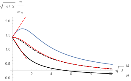
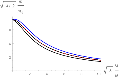
Figure 1: Meson masses in the quenched background as a function of the flux integer $M$ for the lightest meson with excitation integer $n=0$ (left) and for $n=3$ (right). The upper blue (lower black) curves corresponds to the mode $\chi_{-}$ ($\chi_{+}$). The intermediate red curve is the average of the two curves, and the dashed black curve is the WKB estimate (7.24). The two straight lines on the left panel are the first-order results written in (7.21).

To find the mass spectrum of the mesons we must determine the values of $m$ for which there exists a normalizable solution to (7.14). In general this must be done numerically by using the shooting technique, although, we can make analytic estimates using the WKB approximation, which we describe in detail in Appendix D. The result is a tower of solutions with increasing masses which depend on the flux. These masses depend on the location of the tip $r_{*}$, which can be related to the mass of the quarks $m_{q}$ as:

$$m_{q}\,=\,\sqrt{{\lambda\over 2}}\,\,\sigma\,r_{*}\ .$$ (7.15)

In Fig. 1 we illustrate the dependence on the flux of the mass of the lightest state, for the quenched background with $N_{f}=0$. The spectra of the two helicity states are different. The mass splitting obviously vanishes at $Q=0$ and changes with the amount of flux.

For $N_{f}=0$ it is possible to compute analytically the meson mass splitting at first order in $Q$. Indeed, the fluctuation equation at first order in $Q$ for the unflavored background is:

$$\partial_{r}\,\big{[}\,(r^{2}-r_{*}^{2})\partial_{r}\,R_{\pm}\,\big{]}\,+\,{m^{2}\over r^{2}}\,R_{\pm}\,\pm\,2mQ\,{r_{*}^{2}\over r^{3}}\,R_{\pm}\,=\,0.$$ (7.16)

For $Q=0$, Eq. (7.16) can be solved analytically in terms of hypergeometric functions. Let $R_{n}(r)$ be the normalizable regular solutions of (7.16) for $Q=0$; they are given by:

$$R_{n}(r)\,=\,\Big{(}{r_{*}\over r}\Big{)}^{2n+1}\,\,F\left(-n-{1\over 2},-n;1;1-{r^{2}\over r_{*}^{2}}\,\right)\ ,\qquad\qquad n\,=\,0,1,\ldots\ .$$ (7.17)

The corresponding mass levels are:

$${m_{n}\over r_{*}}\,=\,\sqrt{2(n+1)(2n+1)}\ ,\qquad\qquad n\,=\,0,1,\ldots\ .$$ (7.18)

Let us now solve (7.16) at first order in $Q$. We write:

$$R_{\pm,n}(r)\,=\,R_{n}(r)\pm Q\,\delta R_{n}(r)\,+\,{\mathcal{O}}(Q^{2})\ ,$$ (7.19)

where the two signs are in correspondence with the ones in (7.16). The mass levels associated to $R_{\pm,n}$ will be denoted by $m_{\pm,n}$. The lightest regular normalizable modes at first order in $Q$ are given by:

$$R_{\pm,0}(r)\,=\,{r_{*}\over r}\pm Q\,\left[{c\over r}+{1\over\sqrt{2}}\,\Big{(}{r_{*}\over r}\Big{)}^{2}\left(1\,-\,{r\over r_{*}}\,\log\left(1+{r_{*}\over r}\right)\right)\right]\,+\,{\mathcal{O}}(Q^{2})\,\,,$$ (7.20)

with $c$ being an integration constant. The masses for these modes are:

$${m_{\pm,0}\over r_{*}}\,=\,\sqrt{2}\mp\,{3\over 4}\,Q\,+\,{\mathcal{O}}(Q^{2})\ .$$ (7.21)

In Fig. 1 we plot these first-order results and we compare them with the numerical calculations. The first-order correction in the flux can similarly be obtained for the modes with $n\geq 1$, and the general form for the mass splitting is:

$${m_{-,n}-m_{+,n}\over r_{*}}\,=\,{(2n+1)(3+4n)\over 2\,(n+1)\,\pi}\,\left[\,{\Gamma\Big{(}n+{1\over 2}\Big{)}\over\Gamma\big{(}n+1\big{)}}\right]^{2}\,\,Q\,+\,{\mathcal{O}}(Q^{2})\ .$$ (7.22)

It follows from this expression that the first-order mass splitting becomes $4Q/\pi\,+\,{\mathcal{O}}(Q^{2})$ as $n\to\infty$.

As shown in Fig. 1, the mass averaged over the two helicities is well approximated by the WKB method:

$${m_{+,n}+m_{-,n}\over 2}\approx m_{WKB}\ .$$ (7.23)

Let us write the WKB estimate of this helicity average in the unflavored background. By using the values of the WKB masses written in Appendix D, we have:

$${m_{+,n}+m_{-,n}\over 2}\approx{r_{*}\over F\Big{(}-{1\over 2},{1\over 2};1;-Q^{2}\,\Big{)}}\,\sqrt{2(n+1)(2n+1)}\,\,.$$ (7.24)

8 Discussion

In this paper, we initiated a study of D6-brane probes with parity-breaking flux in the ABJM background with unquenched massless flavors. Minkowski embeddings of these probe branes holographically described massive fermions in quantum Hall states. The filling fraction was a half-integer in the quenched case, but received corrections when the dynamics of the sea of massless flavors is included. The conductivities, both in the gapped Minkowski embeddings and in the metallic black hole ones, depended on the parity-breaking flux but also contained a contribution from the dynamical flavors. This was interpreted as an effect of the intrinsic disorder due to quantum fluctuations of the fundamental degrees of freedom.

Despite the complexity of the equations of motion we managed to obtain an explicit, analytic family of supersymmetric solutions with nonzero charge density, electric, and magnetic fields. For these gapped QH solutions, we obtained an analytic expression for the Hall conductivity, which includes the effects of quark loops. We also analyzed the residual $SO_{+}(1,1)$ boost invariance of the system at zero temperature; this is a powerful tool for generating non-supersymmetric solutions with general electric and magnetic fields starting from solutions with either $E$=0 or $B$=0. We also explored the effect of the parity violation on the computation of the meson spectrum. We restricted our analysis to the fluctuations of the gauge field around the zero-temperature supersymmetric configuration in which only the internal gauge field components were switched on.

There remain many open topics for further investigation. Although, we presented here a set of analytic, BPS solutions for a very specific set of parameters, more general solutions with nonzero temperature and arbitrary $d$, $Q$, $E$, and $B$ still need to be studied, probably numerically. A thorough analysis of the thermodynamics and phase structure is needed to provide a complete understanding of this model. For example, we anticipate a phase transition as the temperature is increased from the MN to the black hole embeddings.

The effects of internal flux and the sea of massless quarks are particularly interesting. And, we would also like to understand how the BPS solutions fit in to the complete picture.

Because there are so many possible parameters to vary, it makes sense to start by isolating one or two. A good first step could be to analyze, along the lines of [20], the thermodynamics of the D6-brane probe with only the internal flux, presented in Section 3.2. In the absence of massless flavors, this system is essentially a probe D6-brane in the ABJ background, but with zero worldvolume gauge field. This is another system which deserves a detailed thermodynamic study.

Another interesting problem for the future is the study of flavor branes with internal flux in the ABJM background with unquenched massive quarks presented in [22]. The geometry found in [22] is a running solution flowing between two $AdS$ spaces, in which the control parameter is the mass of the sea quarks. One expects to find conductivities depending on the mass of the dynamical quarks, which interpolate between the values found here (for massless sea quarks) and the unflavored values (for infinitely massive quarks).

In this paper we considered brane probes with electric and magnetic fields in their worldvolume and we have neglected the backreaction of these electromagnetic fields. Computing this backreaction is a very complicated task. One possible intermediate step could be considering the geometry dual to the non-commutative ABJM model, which was found in [35] by applying a TsT duality transformation. By adding internal flux to the probe branes we should be able to find Hall states similar to those found here [36].

We initiated a very limited fluctuation analysis in Section 7, and a more thorough study is needed. One goal would be to compute the full meson dispersion about the BPS solution of Section 6. The lightest neutral excitations of QH fluids are magneto-rotons, collective excitations whose minimum energy is at nonzero momentum. They have been detected in experiments, for example [37], and they have also been found in other holographic probe-brane QH models [38, 39]. Naturally, we would like to know if the spectrum of the model presented here also includes rotons.

Homogeneity-breaking instabilities seem to be a general feature of black hole embeddings in related brane models [43, 40, 41, 42], which are examples of the general type of instability described in [44]. In some cases, examples of spatially-modulated ground states have been found explicitly; for example, see [45, 46, 47, 48]. A thorough analysis of the quasi-normal mode spectrum is needed to determine whether such instabilities exists in this model. If so, the ABJM system, due to its symmetries and other special properties, might afford an ideal laboratory to study inhomogeneous phases.

Another interesting area to explore is alternative quantization of the D6-brane worldvolume gauge field. In a four-dimensional bulk, the gauge field can take Dirichlet, Neumann, or mixed boundary conditions in the UV, and these choices correspond to different boundary CFTs dual to strongly coupled anyon fluids in dynamical gauge fields. In particular, by changing the quantization as in [49, 50, 51], this ABJM system could be turned from a quantum Hall fluid into an anyon superfluid.

Acknowledgments

Y.  B and A. V. R. are funded by the Spanish grant FPA2011-22594, by the Consolider-Ingenio 2010 Programme CPAN (CSD2007-00042), by Xunta de Galicia (Conselleria de Educación, grant INCITE09-206-121-PR and grant PGIDIT10PXIB206075PR), and by FEDER. Y. B. is also supported by the foundation Pedro Barri de la Maza. N. J. is supported by the Academy of Finland grant no. 1268023. D. Z. is funded by the FCT fellowship SFRH/BPD/62888/2009. M. L. is supported by funding from the European Research Council under the European Union’s Seventh Framework Programme (FP7/2007-2013) / ERC Grant agreement no. 268088-EMERGRAV. This work is part of the $\Delta$-ITP consortium and also supported in part by the Foundation for Fundamental Research on Matter (FOM), both are parts of the Netherlands Organization for Scientific Research (NWO) that is funded by the Dutch Ministry of Education, Culture and Science (OCW). Y. B. wants to thank the University of Swansea for hospitality at the final stages of this work. N. J. wishes to thank the hospitality of the Universidade de Santiago de Compostela, especially for the chipirones, while this work was in progress. M. L. would like to thank the University of Helsinki and the Helsinki Institute of Physics for the very warm hospitality, and especially for the reindeer, while this work was being completed.

Appendix A Details of the background geometry

In this appendix we specify the coordinate system we employ to represent the metric and forms of the background. Let us begin with the four-sphere part of the internal metric (2.4). Let $\omega^{i}$ ($i=1,2,3$) be the $SU(2)$ left-invariant one-forms which satisfy $d\omega^{i}={1\over 2}\,\epsilon_{ijk}\,\omega^{j}\wedge\omega^{k}$. Together with a new coordinate $\alpha$, the $\omega^{i}$’s can be used to parameterize the metric of the four-sphere ${\mathbb{S}}^{4}$ as:

$$ds^{2}_{{\mathbb{S}}^{4}}\,=\,d\alpha^{2}\,+\,{\sin^{2}\alpha\over 4}\left[(\omega^{1})^{2}+(\omega^{2})^{2}+(\omega^{3})^{2}\right]\ ,$$ (A.1)

where $0\leq\alpha<\pi$. The $SU(2)$ instanton one-forms $A^{i}$ which fiber the ${\mathbb{S}}^{2}$ over the ${\mathbb{S}}^{4}$ in (2.4) can be written in these coordinates as:

$$A^{i}\,=\,-\sin^{2}\left({\alpha\over 2}\right)\,\,\omega^{i}\,\,.$$ (A.2)

Let us next parametrize the $z^{i}$ coordinates of the ${\mathbb{S}}^{2}$ by means of two angles $\theta$ and $\varphi$ ($0\leq\theta<\pi$, $0\leq\varphi<2\pi$), namely:

$$z^{1}\,=\,\sin\theta\,\cos\varphi\,\,,\qquad\qquad z^{2}\,=\,\sin\theta\,\sin\varphi\,\,,\qquad\qquad z^{3}\,=\,\cos\theta\,\,.$$ (A.3)

Then, one can easily prove that the ${\mathbb{S}}^{2}$ part of the metric (2.4) can be written as:

$$\left(dx^{i}\,+\,\epsilon^{ijk}\,A^{j}\,z^{k}\,\right)^{2}\,=\,(E^{1})^{2}\,+\,(E^{2})^{2}\ ,$$ (A.4)

where $E^{1}$ and $E^{2}$ are the following one-forms:

$$E^{1} = d\theta+\sin^{2}\big{(}{\alpha\over 2}\big{)}\,\left[\sin\varphi\,\omega^{1}-\cos\varphi\,\omega^{2}\right]$$

$$E^{2} = \sin\theta\left[d\varphi-\sin^{2}\big{(}{\alpha\over 2}\big{)}\,\omega^{3}\right]+\sin^{2}\big{(}{\alpha\over 2}\big{)}\,\cos\theta\left[\cos\varphi\,\omega^{1}+\sin\varphi\,\omega^{2}\right]\ .$$ (A.5)

In order to write the explicit expression for $F_{2}$, we first define three new one-forms $S^{i}$ $(i=1,2,3)$ as the following rotated version of the $\omega^{i}$’s:

$$S^{1} = \sin\varphi\,\omega^{1}-\cos\varphi\,\omega^{2}$$

$$S^{2} = \sin\theta\,\omega^{3}-\cos\theta\left(\cos\varphi\,\omega^{1}+\sin\varphi\,\omega^{2}\right)$$

$$S^{3} = -\cos\theta\,\omega^{3}-\sin\theta\left(\cos\varphi\,\omega^{1}+\sin\varphi\,\omega^{2}\right)\ .$$ (A.6)

Next, we define the one-forms ${\cal S}^{\alpha}$ and ${\cal S}^{i}$ as:

$${\cal S}^{\alpha}\,=\,d\alpha\,\,,\qquad\qquad{\cal S}^{i}\,=\,{\sin\alpha\over 2}\,S^{i}\,\,,\qquad(i=1,2,3)\ ,$$ (A.7)

in terms of which the metric of the four-sphere is just $ds^{2}_{{\mathbb{S}}^{4}}=({\cal S}^{\alpha})^{2}+\sum_{i}({\cal S}^{i})^{2}$.

With these definitions, the ansatz for the RR two-form $F_{2}$ for the flavored background is

$$F_{2}\,=\,{k\over 2}\,\,\Big{[}\,\,E^{1}\wedge E^{2}\,-\,\eta\,\big{(}{\cal S}^{\alpha}\wedge{\cal S}^{3}\,+\,{\cal S}^{1}\wedge{\cal S}^{2}\big{)}\,\,\Big{]}\ .$$ (A.8)

Note that the two-form $F_{2}$ is not closed when $\eta\not=1$; $dF_{2}$ is proportional to the charge distribution three-form of the flavor D6-branes. The RR four-form $F_{4}$ is:

$$F_{4}\,=\,{3k\over 4}\,\,\,{(\eta+q)b\over 2-q}\,\,L^{2}\,\,\Omega_{BH_{4}}\ ,$$ (A.9)

where $\Omega_{BH_{4}}$ is the volume-form of the four-dimensional black hole (2.2). The solution is completed by a constant dilaton $\phi$ given by

$$e^{-\phi}\,=\,{b\over 4}\,{\eta+q\over 2-q}\,{k\over L}\ .$$ (A.10)

Let us now spell out the embedding of the D6-brane probe in the background geometry. We first represent the $SU(2)$ left-invariant one-forms $\omega^{i}$ in terms of three angles $\hat{\theta}$, $\hat{\varphi}$, and $\hat{\psi}$ as:

$$\omega^{1} = \cos\hat{\psi}\,d\hat{\theta}+\sin\hat{\psi}\,\sin\hat{\theta}\,d\hat{\varphi}$$

$$\omega^{2} = \sin\hat{\psi}\,d\hat{\theta}-\cos\hat{\psi}\,\sin\hat{\theta}\,d\hat{\varphi}$$

$$\omega^{3} = d\hat{\psi}+\cos\hat{\theta}\,d\hat{\varphi}\,\,.$$ (A.11)

In these coordinates our embedding is defined by the conditions:

$$\hat{\theta}\,,\ \hat{\varphi}\,=\,{\rm constant}\ ,$$ (A.12)

with the coordinate $\theta$ defined in (A.3) being a function of the radial coordinate $r$. The relation of the coordinates defined here with those used in (3.1) to write the internal part of the induced metric is as follows: The angle $\alpha$ here is equal to the one introduced in (A.1), while $\beta$ and $\psi$ are given by

$$\beta\,=\,{\hat{\psi}\over 2}\,\,,\qquad\qquad\psi\,=\,\varphi\,-\,{\hat{\psi}\over 2}\ .$$ (A.13)

It is now easy to check that the pullback of the metric (2.1) to the worldvolume is, indeed, the line element written in (3.1).

A.1 Matching the unflavored ABJ model

Let us now explore our prescription (3.3) in the case of the unflavored model. The main point is that, when $N_{f}=0$, the worldvolume gauge field for the supersymmetric configurations can be understood as induced by a flat NSNS $B_{2}$ field of the bulk, which is proportional to the Kähler form $J$ of ${\mathbb{C}}{\mathbb{P}}^{3}$. When the coefficient multiplying $J$ is appropriately quantized, the corresponding supergravity solution is the dual of the ABJ theory with gauge group $U(N+M)_{k}\times U(N)_{-k}$. We will see that the rank difference $M$ can be identified with the quantization integer in (3.3).

Let us begin our analysis by writing the Kähler form of ${\mathbb{C}}{\mathbb{P}}^{3}$ in our variables:

$$J\,=\,{1\over 4}\,\,\Big{(}\,E^{1}\wedge E^{2}\,-\,\big{(}{\cal S}^{\alpha}\wedge{\cal S}^{3}\,+\,{\cal S}^{1}\wedge{\cal S}^{2}\big{)}\,\Big{)}\ .$$ (A.14)

The pullback of $J$ to the probe brane worldvolume is:

$$\hat{J}\,=\,{\theta^{\prime}\,\sin\theta\over 4}\,dr\wedge\big{[}\,d\psi+\cos\alpha\,d\beta\,\big{]}\,+\,{\cos\theta\sin\alpha\over 4}\,d\alpha\wedge d\beta\ ,$$ (A.15)

and, as claimed, it has the form written in (3.5) if we identify the flux function $a(r)$ with:

$$a(r)\,=-Q\,\cos\theta(r)\ ,$$ (A.16)

where $Q$ is a constant. Actually, one can check that the worldvolume gauge field $F$ (3.5) for this unflavored case can be written in terms of the pullback of $J$ as:

$$F\,=\,4\,L^{2}\,Q\,\hat{J}\,\,.$$ (A.17)

We will see below in Appendix C that the relation (A.16) between the flux and embedding functions is dictated by supersymmetry when $N_{f}=0$. Notice also that the flux function at the tip is just $Q$, as in (3.9).

In the DBI+WZ action for D-branes, the worldvolume gauge field $F$ is always combined additively with the pullback of $B_{2}$. It follows that, in this case, the worldvolume flux can alternatively be thought of as induced by the following NSNS $B_{2}$ field:

$$B_{2}\,=\,4\,Q\,L^{2}\,J\,\,.$$ (A.18)

Notice that $B_{2}$ is a closed two-form, and it has the same form as in the proposed gravity dual of the ABJ model [24] with gauge group $U(N+M)_{k}\times U(N)_{-k}$, where $Q$ is related to $M$. Actually, the integer $M$ is determined by the discrete holonomy of $B_{2}$ on the ${\mathbb{C}}{\mathbb{P}}^{1}$ cycle of the ${\mathbb{C}}{\mathbb{P}}^{3}$ space, which is inherited from the holonomy of the three-dimensional three-form potential of the eleven dimensional supergravity along the torsion cycle of the ${\mathbb{S}}^{7}/{\mathbb{Z}_{k}}$. Let us compute explicitly the integral of the two-form (A.18) along the ${\mathbb{C}}{\mathbb{P}}^{1}$. In our coordinates (see [19]) the ${\mathbb{C}}{\mathbb{P}}^{1}$ is obtained by keeping the coordinates of the ${\mathbb{S}}^{4}$ cycle fixed. Therefore, the pullback of $J$ is just:

$$J_{|_{{\mathbb{C}}{\mathbb{P}}^{1}}}\,=\,{1\over 4}\,\sin\theta\,d\theta\wedge d\varphi\,\,,$$ (A.19)

and thus the integral of $J$ along the ${\mathbb{C}}{\mathbb{P}}^{1}$ is:

$$\int_{{\mathbb{C}}{\mathbb{P}}^{1}}\,J\,=\,\pi\,\,.$$ (A.20)

It follows from (A.18) that:

$$\int_{{\mathbb{C}}{\mathbb{P}}^{1}}\,B_{2}\,=\,4\pi\,L^{2}\,Q\,\,.$$ (A.21)

Let us now use our quantization condition (3.8) and the identification (3.9) to write the period of $B_{2}$ in terms of $k$ and the quantization integer $M$. We get:

$$\int_{{\mathbb{C}}{\mathbb{P}}^{1}}\,B_{2}\,=\,(2\pi)^{2}\,{M\over k}\,\,,$$ (A.22)

which is the fractional holonomy proposed in [24] for the gravity dual of the $U(N+M)_{k}\times U(N)_{-k}$ theory.

The coefficient $Q$ can also be fixed by looking at the Page charge $Q_{4}$ for fractional D2-branes (D4-branes wrapped on a ${\mathbb{C}}{\mathbb{P}}^{1}$ two-cycle), which is given by the following integral over the ${\mathbb{C}}{\mathbb{P}}^{2}$ dual to the ${\mathbb{C}}{\mathbb{P}}^{1}$ where the D4-branes are wrapped:

$$Q_{4}\,=\,{1\over(2\pi)^{3}}\,\int_{{\mathbb{C}}{\mathbb{P}}^{2}}\,\Big{[}F_{4}+B_{2}\wedge F_{2}]\,\,.$$ (A.23)

We require that $Q_{4}$ is equal to our quantization integer $M$, which can then be interpreted as the number of fractional D2-branes. Taking into account (A.18) and that $F_{2}=2k\,J$ for this unflavored case, we get:

$$Q_{4}\,=\,{k\,L^{2}\,Q\over\pi^{3}}\,\int_{{\mathbb{C}}{\mathbb{P}}^{2}}\,J\wedge J\,\,.$$ (A.24)

To compute this integral we use the fact that the equation of the ${\mathbb{C}}{\mathbb{P}}^{2}$ cycle in our coordinates is $\varphi=\theta=\pi/2$ (see Appendix A in [19]), which implies:

$$J\wedge J_{|_{{\mathbb{C}}{\mathbb{P}}^{2}}}\,=\,{1\over 16}\,\sin^{2}{\alpha\over 2}\,\sin\alpha\,\,d\alpha\wedge\omega^{1}\wedge\omega^{2}\,\wedge\omega^{3}\,\,.$$ (A.25)

Then, it follows that:

$$\int_{{\mathbb{C}}{\mathbb{P}}^{2}}\,J\wedge J\,=\,\pi^{2}\,\,.$$ (A.26)

Therefore,

$$Q_{4}\,=\,{k\,L^{2}\,Q\over\pi}\,\,,$$ (A.27)

and the quantization condition $Q_{4}=M$ coincides with the one obtained in (3.8) for $a_{*}\,=\,-Q$.

Appendix B Probe brane equation of motion

Let us consider a D$p$-brane probe propagating in a background of type II supergravity. Let $g_{ij}$ denote the components of the induced metric on the worldvolume:

$$g_{ij}\,=\,g_{mn}\,\partial_{i}\,X^{m}\,\partial_{j}\,X^{n}\,\,,$$ (B.1)

where the $X^{n}$ are coordinates of the ten-dimensional space and $g_{mn}$ is the target space metric of the background. In what follows $m,n,\ldots$ will denote indices of the target space, whereas $i,j,\ldots$ will represent worldvolume indices. Let us denote by $M$ the following matrix:

$$M\,=\,g+F\,\,,$$ (B.2)

where $F=dA$ is the worldvolume gauge field. Then, the action of a D$p$-brane probe can be written as:

$$S_{D_{p}}\,=\,S_{DBI}+S_{WZ}\,\,,$$ (B.3)

where the DBI and WZ terms are:

$$S_{DBI}\,=\,-T_{Dp}\,\int_{{\cal M}_{p+1}}\,d^{p+1}\xi\,\,e^{-\phi}\,\sqrt{-\det M}\,\,,\qquad\qquad S_{WZ}\,=\,T_{Dp}\,\int_{{\cal M}_{p+1}}\,e^{F}\wedge C\,\,,$$ (B.4)

with $T_{Dp}$ being the D$p$-brane tension (from now on in this appendix we will take $T_{Dp}=1$) and $C=\sum_{r}C_{r}$ is the sum of RR potentials. In order to write the equations of motion derived from this action following the analysis of Section 2 of [52], let us consider the inverse $M^{-1}=[M^{ij}]$ of the matrix $M=[M_{ij}]$ and let us decompose $M^{-1}$ in its symmetric and antisymmetric parts as:

$$M^{-1}\,=\,{\cal G}^{-1}\,+\,{\cal J}\,\,,$$ (B.5)

where ${\cal J}=[{\cal J}^{ij}]$ is the antisymmetric component of $M^{-1}$ and ${\cal G}^{-1}=[{\cal G}^{ij}]$ is the inverse open string metric. Then, the equation of motion of the gauge field component $A_{j}$ is [52]:

$$\partial_{j}\Big{(}e^{-\phi}\,\sqrt{-\det M}\,{\cal J}^{ji}\Big{)}\,=\,j^{i}\,\,,$$ (B.6)

where the source current for the gauge field $j^{i}$ is given by:

$$j^{i}\equiv{\delta S_{WZ}\over\delta A_{i}}\,\,.$$ (B.7)

Moreover, the equation for the scalar field $X^{m}$ becomes [52]:

$$-\partial_{i}\Big{(}e^{-\phi}\,\sqrt{-\det M}\,{\cal G}^{ij}\,\partial_{j}\,X^{n}\,g_{nm}\Big{)}\,\,$$

$$\qquad\qquad+\sqrt{-\det M}\,\Big{(}{e^{-\phi}\over 2}\,{\cal G}^{ji}\,\partial_{i}\,X^{n}\,\partial_{j}\,X^{p}\,g_{np,m}\,-\,e^{-\phi}\,\partial_{m}\,\phi\Big{)}\,=\,j_{m}\,\,,\qquad\qquad$$ (B.8)

where the source for the scalar $X^{m}$ is:

$$j_{m}\equiv{\delta S_{WZ}\over\delta X^{m}}\,\,.$$ (B.9)

B.1 Currents for the D6-brane

Let us write the form of the currents for the case of a D6-brane probe. In this case, the WZ term of the action is:

$$S_{WZ}\,=\,\int_{{\cal M}_{7}}\,\left(\hat{C}_{7}\,+\,\hat{C}_{5}\wedge F\,+\,{1\over 2}\,\hat{C}_{3}\wedge F\wedge F\,+\,{1\over 6}\hat{C}_{1}\wedge F\wedge F\wedge F\right)\ .$$ (B.10)

Let us perform a general variation of the worldvolume gauge field $F\to F+d(\delta A)$, under which $S_{WZ}$ varies as:

$$\delta S_{WZ}\,=\,\int_{{\cal M}_{7}}\,\left(\hat{C}_{5}\,+\,\hat{C}_{3}\wedge F\,+\,{1\over 2}\,\hat{C}_{1}\wedge F\wedge F\right)\wedge d(\delta A)\ .$$ (B.11)

In order to compute the current associated to the worldvolume gauge field, we use the fact that, for any odd-dimensional form ${\cal O}$, one has

$${\cal O}\wedge d(\delta A)\,=\,d{\cal O}\wedge\delta A\,-\,d({\cal O}\wedge\delta A)\ .$$ (B.12)

The total derivative generates a boundary term which vanishes since we are assuming that $A$ is fixed at the boundary in the variational process. Taking into account that, with our notation $F_{4}=-dC_{3}$, we get:

$$\delta S_{WZ}\,=\,\int_{{\cal M}_{7}}\,\left(\hat{F}_{6}\,-\,\hat{F}_{4}\wedge F\,+\,{1\over 2}\,\hat{F}_{2}\wedge F\wedge F\right)\wedge\delta A\ .$$ (B.13)

Then, the gauge current along the worldvolume direction $i$ is given by the expression:

$$j^{i}\,d^{7}\xi\,=\,\left(\hat{F}_{6}\,-\,\hat{F}_{4}\wedge F\,+\,{1\over 2}\,\hat{F}_{2}\wedge F\wedge F\right)\wedge d\xi^{i}\ .$$ (B.14)

In order to compute the source current $j_{m}$ for $X^{m}$, we should vary in (B.10) the scalars which enter the pullback of the RR potentials. It turns out that the final expression can be written in a rather simple form, which we will now spell out. Let $V=V^{m}\,{\partial\over\partial X^{m}}$ be any vector field in target space. The interior product of $V$ with a $p$-form $\omega$ is a $(p-1)$-form $\iota_{V}\omega$ defined as follows. Let $\omega$ be:

$$\omega\,=\,{1\over p!}\,\omega_{n_{1},\ldots,n_{p}}\,dX^{n_{1}}\wedge\cdots\wedge dX^{n_{p}}\,\,.$$ (B.15)

Then, $\iota_{V}\omega$ is given by:

$$\iota_{V}\omega\,=\,{1\over(p-1)!}\,V^{m}\,\omega_{m,m_{1},\ldots,m_{p-1}}\,dX^{m_{1}}\wedge\cdots\wedge dX^{m_{p-1}}\,\,.$$ (B.16)

Let $\iota_{m}\omega$ denote the interior product of $\omega$ and the vector $\partial/\partial X^{m}$:

$$\iota_{m}\omega\,\equiv\,\iota_{{\partial\over\partial X^{m}}}\omega\,\,.$$ (B.17)

Then, the current $j_{m}$, corresponding to the scalar $X^{m}$, can be written as:

$$j_{m}\,d^{7}\xi\,=\,\widehat{\iota_{m}F_{8}}\,+\,\widehat{\iota_{m}F_{6}}\wedge F\,-\,{1\over 2}\,\widehat{\iota_{m}F_{4}}\wedge F\wedge F\,+\,{1\over 6}\,\widehat{\iota_{m}F_{2}}\wedge F\wedge F\wedge F\,\,,$$ (B.18)

where the hat denotes the pullback of the different $\iota_{m}F_{r}$ to the worldvolume. In (B.18) $F_{8}$ and $F_{6}$ are defined as Hodge duals of $F_{2}$ and $F_{4}$, respectively, i.e., $F_{8}=-*F_{2}$ and $F_{6}=-*F_{4}$.

Notice that we have derived the expressions of $j^{i}$ and $j_{m}$ from the action (B.10), where we have assumed the existence of the RR potentials $C_{r}$. In the case of backreacting flavor some Bianchi identities are violated and, as a consequence, some of the RR potentials do not exist. However, the currents $j^{i}$ and $j_{m}$ (and the corresponding equations of motion) only depend on the RR field strengths and their pullbacks, and then they can be generalized to the case in which we include the backreaction. This is the point of view we will adopt in what follows.

B.2 The equations of motion for our ansatz

We now write explicitly the equations of motion for the D6-brane with a gauge potential $A$ as the one written in (3.13). We will also assume that the embedding is defined by the conditions (A.12) with $\theta=\theta(r)$ being a function of $r$ to be determined. The set of worldvolume coordinates we will employ is:

$$\xi^{i}\,=\,(t,x,y,r,\alpha,\beta,\psi)\,\,,$$ (B.19)

where $\alpha$, $\beta$, and $\psi$ are the angles defined in (A.1) and (A.13). First of all, let us write the non-zero components of the worldvolume gauge field strength $F$ corresponding to the potential (3.13):

$$F_{t\,x}\,=\,L^{2}\,E\,\,,\qquad\qquad F_{x\,y}\,=\,L^{2}\,B\,\,,$$

$$F_{r\,t}\,=\,L^{2}\,a_{0}^{\prime}\,\,,\qquad\qquad F_{r\,x}\,=\,L^{2}\,a_{x}^{\prime}\,\,,\qquad\qquad F_{r\,y}\,=\,L^{2}\,a_{y}^{\prime}\,\,,$$

$$F_{r\,\psi}\,=\,L^{2}\,a^{\prime}\,\,,\qquad\qquad F_{r\,\beta}\,=\,L^{2}\,a^{\prime}\cos\alpha\,\,,\qquad\qquad F_{\alpha\,\beta}\,=\,-L^{2}\,a\,\sin\alpha\,\,,\qquad\qquad\qquad$$ (B.20)

where the prime denotes the derivative with respect to the radial variable. Notice that, in our ansatz, isotropy in the $x-y$ plane is explicitly broken by the electric field in the $x$-direction.

We will start by computing the different components of the currents appearing in (B.6) and (B.8). It is straightforward to prove that $\hat{F}_{6}=0$, and it therefore does not contribute to $j^{i}$ and $j_{m}$. The non-vanishing components of the gauge current $j^{i}$ are:

$$j^{t}\,=\,{kL^{4}\over 2}\,B\,\sin\alpha\,(\eta\,\cos\theta\,a^{\prime}\,-\,a\,\sin\theta\,\theta^{\prime})\,\,,$$

$$j^{y}\,=\,{kL^{4}\over 2}\,E\,\sin\alpha\,(\eta\,\cos\theta\,a^{\prime}\,-\,a\,\sin\theta\,\theta^{\prime})\,\,,$$

$$j^{\psi}\,=\,{kL^{4}\over 2}\,\sin\alpha\,\Bigg{(}{3b\over 2}\,{\eta+q\over 2-q}\,r^{2}\,a\,-\,\eta\,(B\,a_{0}^{\prime}+E\,a_{y}^{\prime})\cos\theta\Bigg{)}\,\,.$$ (B.21)

We now work out the current for the three transverse scalars. First we compute the interior products of $F_{8}$ with the tangent vectors along the three scalar directions $m=\theta,\hat{\theta},\hat{\varphi}$. We find:

$$\widehat{\iota_{\theta}F_{8}}\,=\,-{(3-2b)(q+\eta)q\over 8b^{3}(2-q)}\,kL^{6}\,\sin\alpha\,r^{2}\,\sin(2\theta)\,\,d^{7}\xi\,\,.$$ (B.22)

Moreover, the product of $F_{8}$ with the other two tangent vectors gives a result proportional to $\widehat{\iota_{\theta}F_{8}}$:

$$\widehat{\iota_{\hat{\theta}}F_{8}}\,=\,-\sin^{2}\Big{(}{\alpha\over 2}\Big{)}\,\sin(\beta-\psi)\,\widehat{\iota_{\theta}F_{8}}\,\,,\qquad\widehat{\iota_{\hat{\varphi}}F_{8}}\,=\,\sin\hat{\theta}\sin^{2}\Big{(}{\alpha\over 2}\Big{)}\,\cos(\beta-\psi)\,\widehat{\iota_{\theta}F_{8}}\,\,.$$ (B.23)

We already mentioned that $F_{6}$ does not contribute since its pullback is zero. It is also immediate to check that $F_{4}$ does not have components along the transverse scalars and will not contribute to $j_{m}$. The contribution of $F_{2}$ to $j_{\theta}$ is determined by:

$${1\over 6}\,\widehat{\iota_{\theta}F_{2}}\wedge F\wedge F\wedge F\,=\,{kL^{6}\over 2}\,\sin\alpha\,a\,\sin\theta\,(B\,a_{0}^{\prime}\,+\,E\,a_{y}^{\prime})\,\,d^{7}\xi\,\,,$$ (B.24)

while the result for the other scalars are:

$$\widehat{\iota_{\hat{\theta}}F_{2}}\wedge F\wedge F\wedge F\,=\,-\sin^{2}\Big{(}{\alpha\over 2}\Big{)}\,\sin(\beta-\psi)\,\widehat{\iota_{\theta}F_{2}}\wedge F\wedge F\wedge F\,\,,$$

$$\widehat{\iota_{\hat{\varphi}}F_{2}}\wedge F\wedge F\wedge F\,=\,\sin\hat{\theta}\sin^{2}\Big{(}{\alpha\over 2}\Big{)}\,\cos(\beta-\psi)\,\widehat{\iota_{\theta}F_{2}}\wedge F\wedge F\wedge F\,\,.$$ (B.25)

Notice that the proportionality factors in (B.23) and (B.25) are the same. Thus, the current for the scalar $\theta$ becomes:

$$j_{\theta}\,=\,-{kL^{6}\over 2}\,\sin\alpha\,\sin\theta\,\Bigg{(}{(3-2b)(q+\eta)q\over 2\,b^{3}(2-q)}\,r^{2}\cos\theta\,-\,a\,(B\,a_{0}^{\prime}\,+\,E\,a_{y}^{\prime})\,\Bigg{)}\,\,.$$ (B.26)

Moreover, the other two components of $j_{m}$ are:

$$j_{\hat{\theta}}\,=\,-\sin^{2}\Big{(}{\alpha\over 2}\Big{)}\,\sin(\beta-\psi)\,j_{\theta}\,\,,\qquad j_{\hat{\varphi}}\,=\,\sin\hat{\theta}\,\sin^{2}\Big{(}{\alpha\over 2}\Big{)}\,\cos(\beta-\psi)\,\,j_{\theta}\,\,.$$ (B.27)

Let us now finally write the equations of motion for the different gauge field components and scalars. We have to compute the different components of the antisymmetric tensor ${\cal J}^{ij}$, as well as the elements of the inverse open string metric ${\cal G}^{ij}$. This calculation is straightforward (although rather tedious in some cases) and we limit ourselves to give the final result for the equations. The equation of $A_{t}$ is:

$${q+\eta\over 2b(2-q)}\,\partial_{r}\Bigg{[}{\sqrt{h}\,\sqrt{q^{2}+b^{4}\,a^{2}}\over\sqrt{\Delta}\sqrt{(B^{2}+r^{4})h-E^{2}}}\,\sin^{2}\theta\,\big{[}B(B\,a_{0}^{\prime}\,+\,E\,a_{y}^{\prime})\,+r^{4}\,a_{0}^{\prime}\big{]}\Bigg{]}\,\,$$

$$\qquad\qquad\qquad\qquad-B(\eta\,\cos\theta\,a^{\prime}-a\,\sin\theta\,\theta^{\prime})\,=\,0\,\,,$$ (B.28)

where $\Delta$ is the quantity defined in (3.16). The equation for $A_{x}$ can be integrated once ($a_{x}$ is a cyclic variable) to give the following equation for $a_{x}^{\prime}$:

$$r^{4}\,h^{{3\over 2}}\,\sin^{2}\theta\,{\sqrt{q^{2}+b^{4}\,a^{2}}\,a_{x}^{\prime}\over\sqrt{\Delta}\,\sqrt{(B^{2}+r^{4})h-E^{2}}}\,=\,{\rm constant}\,\,.$$ (B.29)

The equation for $A_{y}$ is also non-trivial and given by:

$${q+\eta\over 2b(2-q)}\,\partial_{r}\Bigg{[}{\sqrt{h}\,\sqrt{q^{2}+b^{4}\,a^{2}}\over\sqrt{\Delta}\sqrt{(B^{2}+r^{4})h-E^{2}}}\,\sin^{2}\theta\,\big{[}E(B\,a_{0}^{\prime}\,+\,E\,a_{y}^{\prime})\,-r^{4}\,h\,a_{y}^{\prime}\big{]}\Bigg{]}\,\,$$

$$\qquad\qquad\qquad\qquad-E(\eta\,\cos\theta\,a^{\prime}-a\,\sin\theta\,\theta^{\prime})\,=\,0\,\,.$$ (B.30)

It is easy to demonstrate that the equations for $A_{r}$, $A_{\alpha}$, and $A_{\beta}$ are trivially satisfied by our ansatz. The only non-trivial equation for the gauge field that remains to write is the one corresponding to $A_{\psi}$, which is:

$$\partial_{r}\Bigg{[}{r^{2}\,\sqrt{h}\,\sqrt{q^{2}+b^{4}\,a^{2}}\,\sqrt{(B^{2}+r^{4})h-E^{2}}\over\sqrt{\Delta}}\,a^{\prime}\Bigg{]}-{\sqrt{\Delta}\,\sqrt{(B^{2}+r^{4})h-E^{2}}\over\sqrt{h}\,\sqrt{q^{2}+b^{4}\,a^{2}}}\,a\,\,$$

$$\qquad\qquad\qquad\qquad+3r^{2}a\,-\,{2(2-q)\,\eta\over b(q+\eta)}\,(B\,a_{0}^{\prime}\,+\,E\,a_{y}^{\prime})\cos\theta=0\,\,.$$ (B.31)

Finally, one can prove that the three equations for the transverse scalars $\theta$, $\hat{\theta}$, and $\hat{\varphi}$ are the same, namely:

$$\partial_{r}\Bigg{[}{r^{2}\,\sin^{2}\theta\,\sqrt{h}\,\sqrt{q^{2}+b^{4}\,a^{2}}\,\sqrt{(B^{2}+r^{4})h-E^{2}}\over\sqrt{\Delta}}\,\theta^{\prime}\Bigg{]}$$

$$\qquad\qquad-\,{\sqrt{q^{2}+b^{4}\,a^{2}}\,\sqrt{(B^{2}+r^{4})h-E^{2}}\over\sqrt{h}\,\sqrt{\Delta}}\big{[}\Delta\,-\,b^{4}\,r^{2}\,h\,a^{\prime\,2}\big{]}\cot{\theta}\qquad$$

$$\qquad-(3-2b)\,q\,r^{2}\,\sin\theta\cos\theta\,+\,{2b^{3}(2-q)\over q+\eta}\,a\,\sin\theta\,(B\,a_{0}^{\prime}\,+\,E\,a_{y}^{\prime})\,=\,0\,\,.\qquad\qquad$$ (B.32)

Eq. (B.29) allows us to eliminate $a_{x}^{\prime}$, after which we have four second-order, coupled differential equations (B.28)-(B.32) for four radial functions of $a_{0}$, $a_{y}$, $a$, and $\theta$. Solving this system in general is a quite formidable task. For this reason it is worth to look for simplifications and partial integrations. Notice that (B.28) and (B.30) present some electric-magnetic symmetry. Actually, by combining these equations one easily finds the following constant of motion:

$${r^{4}\,\sqrt{h}\,\sqrt{q^{2}+b^{4}\,a^{2}}\over\sqrt{\Delta}\sqrt{(B^{2}+r^{4})h-E^{2}}}\,\sin^{2}\theta\,\big{[}E\,a_{0}^{\prime}\,+h\,B\,a_{y}^{\prime}\big{]}\,=\,{\rm constant}\,\,,$$ (B.33)

which could be used to eliminate $a_{0}^{\prime}$ or $a_{y}^{\prime}$ from the system of equations. Moreover, in the unflavored case ($\eta=b=q=1$), the last two terms in (B.28) and (B.30) can be combined to construct the radial derivative of $a\cos\theta$, which leads to two constants of motion. In this unflavored case, $a_{0}$ and $a_{y}$ are cyclic variables and can be eliminated.

Appendix C Kappa symmetry analysis

The kappa symmetry matrix for a D$p$-brane in the type IIA theory is given by:

$$d^{p+1}\,\zeta\,\Gamma_{\kappa}\,=\,{1\over\sqrt{-\det(g+F)}}\,e^{F}\wedge X\,\,,$$ (C.1)

where $g$ is the induced metric, $\zeta^{\alpha}$ ($\alpha=0,\ldots,p)$ are a set of worldvolume coordinates and $X$ is the polyform matrix:

$$X\,=\,\sum_{n}\,\gamma_{2n+1}\,\big{(}\Gamma_{11}\big{)}^{n+1}\,\,,$$ (C.2)

with $\gamma_{2n+1}$ being the $(2n+1)$-form whose components are the antisymmetrized products of the induced Dirac matrices $\gamma_{\mu}$:

$$\gamma_{2n+1}\,=\,{1\over(2n+1)!}\,\gamma_{\mu_{1}\cdots\mu_{2n+1}}\,\,d\zeta^{\mu_{1}}\,\wedge\cdots\wedge d\zeta^{\mu_{2n+1}}\,\,.$$ (C.3)

In particular, we are interested in the case of a D6-brane with a flux across a (non-compact) four-cycle. The corresponding kappa symmetry matrix takes the form:

$$d^{7}\,\zeta\,\Gamma_{\kappa}\,=\,{1\over\sqrt{-\det(g+F)}}\,\Big{[}\,\gamma_{(7)}\,+\,F\wedge\gamma_{(5)}\,\Gamma_{11}\,+\,{1\over 2}\,F\wedge F\wedge\gamma_{(3)}\,+\,{1\over 6}\,F\wedge F\wedge F\wedge\gamma_{(1)}\,\Gamma_{11}\Big{]}\,\,.$$ (C.4)

Let us now study the conditions imposed by kappa symmetry in the case in which the embedding is determined by the conditions (A.12), the worldvolume gauge field takes the form (3.13) with $a_{x}=0$, and the background is the zero-temperature supergravity solution of [19]. We begin by computing the pullbacks of the left-invariant $SU(2)$ one-forms $\omega^{i}$ of (A.11) in the $\alpha$, $\beta$, and $\psi$ variables:

$$\hat{\omega}^{1}\,=\,\hat{\omega}^{2}\,=\,0\,\,,\qquad\qquad\hat{\omega}^{3}\,=\,2d\beta\,\,,$$ (C.5)

whereas those of ${\cal S}^{i}$ and $E^{i}$ are:

$$\hat{\cal S}^{\alpha}\,=\,d\alpha\,\,,\qquad\hat{\cal S}^{1}\,=\,0\,\,,\qquad\hat{\cal S}^{2}\,=\,\sin\alpha\sin\theta\,d\beta\,\,,\qquad\hat{\cal S}^{3}\,=\,-\sin\alpha\cos\theta\,d\beta\,\,,\qquad$$

$$\hat{E}^{1}\,=\,\theta^{\prime}\,dr\,\,,\qquad\qquad\hat{E}^{2}\,=\,\sin\theta\,(d\psi+\cos\alpha\,d\beta)\,\,.$$ (C.6)

The pullbacks of the frame one-forms used in Appendix B of [19] are:

$$\hat{e}^{\mu}\,=\,L\,r\,dx^{\mu}\,\,,\qquad\qquad\hat{e}^{3}\,=\,{L\over r}\,dr\,\,,\qquad\qquad\hat{e}^{4}\,=\,{\sqrt{q}\over b}\,L\,d\alpha\,\,,\qquad\qquad\qquad\qquad$$

$$\hat{e}^{5}\,=\,0\,\,,\qquad\qquad\hat{e}^{6}\,=\,L\,{\sqrt{q}\over b}\,\sin\alpha\sin\theta\,d\beta\,\,,\qquad\qquad\hat{e}^{7}\,=\,-L\,{\sqrt{q}\over b}\,\sin\alpha\cos\theta\,d\beta\,\,,$$

$$\hat{e}^{8}\,=\,{L\over b}\,\theta^{\prime}\,dr\,\,,\qquad\hat{e}^{9}\,=\,{L\over b}\,\sin\theta\,(d\psi+\cos\alpha\,d\beta)\,\,.$$ (C.7)

The corresponding induced gamma matrices become:

$$\gamma_{x^{\mu}}\,=\,L\,r\,\Gamma_{\mu}\,\,,\qquad\qquad\gamma_{r}\,=\,{L\over r}\,\Big{(}\,\Gamma_{3}\,+\,{r\over b}\,\theta^{\prime}\,\Gamma_{8}\,\Big{)}\,\,,\qquad\qquad\gamma_{\alpha}\,=\,L\,{\sqrt{q}\over b}\,\,\,\Gamma_{4}\,\,,\qquad\qquad$$

$$\gamma_{\beta}\,=\,L\,{\sqrt{q}\over b}\,\sin\alpha\sin\theta\,\,\Big{[}\,\Gamma_{6}-\cot\theta\,\Gamma_{7}+{\cot\alpha\over\sqrt{q}}\,\Gamma_{9}\,\Big{]}\,\,,\qquad\qquad\gamma_{\psi}\,=\,{L\,\sin\theta\over b}\,\Gamma_{9}\,\,.$$ (C.8)

Let us next compute the different contributions on the right-hand side of (C.4). First of all we notice that:

$$\gamma_{(7)}\,=\,d^{7}\,\zeta\,\,\gamma_{*}\,\,,$$ (C.9)

where $\gamma_{*}$ is the antisymmetrized product of all induced gamma matrices, namely:

$$\gamma_{*}\,=\,\gamma_{t\,x\,y\,r\,\alpha\,\beta\,\psi}\,\,.$$ (C.10)

In terms of flat 10d matrices, $\gamma_{*}$ can be written as:

$$\gamma_{*}\,=\,{q\over b^{3}}\,L^{7}\,r^{2}\,\sin\alpha\,\sin^{2}\theta\,\,\Gamma_{012}\,\,\Big{(}\,\Gamma_{3}\,+\,{r\,\theta^{\prime}\over b}\,\Gamma_{8}\,\Big{)}\,\Gamma_{4}\,\Big{(}\,\Gamma_{6}\,-\,\cot\theta\,\Gamma_{7}\,\Big{)}\,\Gamma_{9}\,\,.$$ (C.11)

With our notation, the supersymmetric embeddings are those that satisfy $\Gamma_{\kappa}\,\epsilon\,=\,-\epsilon$, where $\epsilon$ is a Killing spinor of the background. To implement this relation we impose that $\epsilon$ satisfies the projection corresponding to a D2-brane, i.e.,

$$\Gamma_{012}\,\epsilon\,=\,-\epsilon\,\,.$$ (C.12)

We also impose that $\epsilon$ satisfies the generic projections found in Appendix B of [19] for a generic ABJM-like geometry (Eqs. (B.4) and (B.14) in [19]):

$$\Gamma_{47}\,\epsilon\,=\,\Gamma_{56}\,\epsilon\,=\,\Gamma_{89}\,\epsilon\,\,,\qquad\qquad\Gamma_{3458}\,\epsilon\,=\,-\,\epsilon\,\,.$$ (C.13)

From these projections it follows that:

$$\Gamma_{3469}\,\epsilon\,=\,-\Gamma_{8479}\,\epsilon\,=\,\epsilon\,\,,\qquad\qquad\Gamma_{3479}\,\epsilon\,=\,\Gamma_{8469}\epsilon\,=\,-\Gamma_{38}\,\epsilon\,\,.$$ (C.14)

Using (C.12) and (C.13), $\gamma_{*}\,\epsilon$ reduces to:

$$\gamma_{*}\,\epsilon\,=\,-{q\over b^{3}}\,L^{7}\,r^{2}\,\sin\alpha\,\sin^{2}\theta\,\,\left[\,1\,+\,{r\,\theta^{\prime}\over b}\,\cot\theta\,+\,\Big{(}\cot\theta\,-\,{r\,\theta^{\prime}\over b}\,\Big{)}\,\Gamma_{38}\,\right]\epsilon\ .$$ (C.15)

From the condition that $\gamma_{*}$ acts diagonally on $\epsilon$ (i.e., $\gamma_{*}$ acts on $\epsilon$ as a matrix proportional to the unit matrix), we get the following equation for the embedding angle:

$$r\,\theta^{\prime}\,=\,b\,\cot\theta\,\,.$$ (C.16)

Moreover, when (C.16) and the projections (C.12) and (C.13) hold, $\gamma_{(7)}$ acts on $\epsilon$ as:

$$\gamma_{(7)}\,\epsilon\,=\,-d^{7}\,\zeta\,{q\over b^{3}}\,L^{7}\,r^{2}\,\sin\alpha\,\epsilon\,\,.$$ (C.17)

Let us now study the terms in (C.4) that are linear in the worldvolume gauge field $F$. Let us write these terms as:

$$F\wedge\gamma_{(5)}\Gamma_{11}\,=\,d^{7}\zeta\,\big{[}\,\Gamma^{flux}+\Gamma^{Min}\,\big{]}\,\,,$$ (C.18)

where $\Gamma^{flux}$ contains the contributions of the components of $F$ along the internal directions and $\Gamma^{Min}$ is the contribution of the components of $F$ with legs along the Minkowski spacetime. It is readily verified that:

$$\Gamma^{flux}\,=\,\gamma_{t\,x\,y}\,\Gamma_{11}\,\Big{[}\,\gamma_{\alpha\,\beta}\,F_{r\,\psi}\,-\,\gamma_{\alpha\psi}\,F_{r\,\beta}\,+\,\gamma_{r\psi}\,F_{\alpha\,\beta}\,\Big{]}\,\,.$$ (C.19)

The antisymmetric products of induced gamma matrices appearing on (C.19) can be straightforwardly computed from (C.8):

$$\gamma_{\alpha\,\beta}\,=\,{q\over b^{2}}\,L^{2}\,\,\sin\alpha\,\sin\theta\,\Big{[}\Gamma_{46}\,-\,\cot\theta\,\Gamma_{47}\,+\,{\cot\alpha\over\sqrt{q}}\,\,\Gamma_{49}\,\Big{]}\,\,,$$

$$\gamma_{\alpha\psi}\,=\,{\sqrt{q}\over b^{2}}\,L^{2}\,\sin\theta\,\Gamma_{49}\,\,,$$

$$\gamma_{r\psi}\,=\,{L^{2}\over b}\,{\sin\theta\over r}\,\Big{[}\,\Gamma_{39}\,+\,{r\,\theta^{\prime}\over b}\,\Gamma_{89}\,\Big{]}\,\,,$$ (C.20)

On the other hand, $\Gamma^{Min}$ is given by:

$$\Gamma^{Min}\,=\,L^{2}\,\Big{(}E\,\gamma_{yr}\,-\,a_{0}^{\prime}\,\gamma_{xy}\,+\,B\,\gamma_{tr}\,-\,a_{y}^{\prime}\,\gamma_{tx}\Big{)}\,\gamma_{\alpha\beta\psi}\,\Gamma_{11}\,\,.$$ (C.21)

The products of the induced Dirac matrices needed to compute $\Gamma^{Min}$ are:

$$\gamma_{yr}\,=\,L^{2}\,\Big{[}\Gamma_{23}\,+\,{r\over b}\,\theta^{\prime}\,\Gamma_{28}\Big{]}\,\,,\qquad\qquad\gamma_{xy}\,=\,L^{2}\,r^{2}\,\Gamma_{12}\,\,,$$

$$\gamma_{tr}\,=\,L^{2}\,\Big{[}\Gamma_{03}\,+\,{r\over b}\,\theta^{\prime}\,\Gamma_{08}\Big{]}\,\,,\qquad\qquad\gamma_{tx}\,=\,L^{2}\,r^{2}\,\Gamma_{01}\,\,,$$

$$\gamma_{\alpha\beta\gamma}\,=\,L^{3}\,{q\over b^{3}}\,\sin\alpha\sin^{2}\theta\,\Big{(}\Gamma_{469}\,-\,\cot\theta\,\Gamma_{479}\Big{)}\,\,.$$ (C.22)

A quick inspection of the different terms appearing in $\Gamma^{flux}\epsilon$ and $\Gamma^{Min}\epsilon$ reveals that, after using the projections (C.12) and (C.13), all terms contain products of $\Gamma$ matrices and there are no terms containing the unit matrix. Therefore, to implement the condition $\Gamma_{\kappa}\,\epsilon=-\epsilon$ we should require that $\Gamma^{flux}\epsilon=\Gamma^{Min}\epsilon=0$. By combining (C.19) and (C.20) we find that the product of $\Gamma$’s contained in $\Gamma^{flux}\,\epsilon$ is:

$${1\over L^{4}}\,\,\Big{[}\,\gamma_{\alpha\beta}\,F_{r\,\psi}\,-\,\gamma_{\alpha\psi}\,F_{r\,\beta}\,+\,\gamma_{r\psi}\,F_{\alpha\beta}\,\Big{]}\,\epsilon\,=\,{\sin\alpha\,\sin\theta\over b}\,\Big{(}{q\over b}\,a^{\prime}\,+\,{a\over r}\Big{)}\,\Gamma_{46}\,\epsilon\,$$

$$\qquad\qquad\qquad\qquad\qquad-{\sin\alpha\over b^{2}}\,\Big{(}q\cos\theta\,a^{\prime}\,+\,\sin\theta\,\theta^{\prime}\,a\Big{)}\,\Gamma_{47}\,\epsilon\,\,.$$ (C.23)

After using the equation (C.16) satisfied by the angle $\theta(r)$, we find that $\Gamma^{flux}\epsilon=0$ if the flux function $a(r)$ satisfies the following first-order equation:

$${a^{\prime}\over a}\,=\,-{b\over q\,r}\,\,.$$ (C.24)

When $E=B=0$ and $a_{0}^{\prime}=a_{y}^{\prime}=0$, Eqs. (C.16) and (C.24) guarantee that the embedding preserves two of the four supersymmetries of the background. If this is not the case, we should continue analyzing the remaining terms in $\Gamma_{\kappa}$. From (C.21) and (C.22) we get:

$${1\over L^{7}}\,\Gamma^{Min}\,\epsilon = {q\over b^{3}}\,\sin\alpha\,\sin^{2}\theta\,\left[E\left(\Gamma_{23}+{r\over b}\theta^{\prime}\,\Gamma_{28}\right)+B\left(\Gamma_{03}+{r\over b}\,\theta^{\prime}\,\Gamma_{08}\right)-r^{2}\,a_{0}^{\prime}\,\Gamma_{12}-r^{2}\,a_{y}^{\prime}\,\Gamma_{01}\right]\,$$ (C.25)

$$\qquad\qquad\qquad\qquad\qquad\qquad\times\Big{(}\Gamma_{469}\,-\,\cot\theta\,\Gamma_{479}\Big{)}\,\Gamma_{11}\,\epsilon\,\,.$$

After using the projections (C.13) we can write the action of $\Gamma^{Min}$ on the Killing spinor $\epsilon$ as:

$${1\over L^{7}}\,\Gamma^{Min}\,\epsilon = {q\over b^{3}}\,\sin\alpha\,\sin^{2}\theta\,\Bigg{[}(E\Gamma_{2}+B\Gamma_{0})\left[1+{r\theta^{\prime}\over b}\cot\theta+\left(\cot\theta-{r\theta^{\prime}\over b}\right)\,\Gamma_{38}\right]\Gamma_{11}\,$$ (C.26)

$$\qquad\qquad\qquad\qquad+\Big{(}a_{0}^{\prime}\,\Gamma_{2}\,-\,a_{y}^{\prime}\,\Gamma_{0}\Big{)}\,r^{2}\,(1+\cot\theta\,\Gamma_{38})\,\Gamma_{13}\,\Gamma_{11}\,\Bigg{]}\epsilon\,\,.$$

Using the BPS equation for $\theta$ (C.16), we can rewrite this last expression as:

$${1\over L^{7}}\Gamma^{Min}\,\epsilon = {q\over b^{3}}\sin\alpha\,\left[(E\Gamma_{2}+B\Gamma_{0})\Gamma_{11}+\big{(}a_{0}^{\prime}\Gamma_{2}-a_{y}^{\prime}\Gamma_{0}\big{)}r^{2}\sin^{2}\theta(1+\cot\theta\,\Gamma_{38})\,\Gamma_{13}\Gamma_{11}\right]\epsilon\,\,.$$

To ensure that $\Gamma^{Min}\,\epsilon=0$ we first impose one of the following two extra projections on $\epsilon$:

$$\Gamma_{02}\,\epsilon\,=\,\pm\epsilon\,\,.$$ (C.28)

Notice that the conditions (C.28) are compatible with the projections (C.12) and (C.13) that we have imposed so far. We get

$${1\over L^{7}}\Gamma^{Min}\,\epsilon={q\over b^{3}}\sin\alpha\,\big{[}(E\mp B)\Gamma_{2}\Gamma_{11}+\big{(}a_{0}^{\prime}\pm a_{y}^{\prime}\big{)}r^{2}\sin^{2}\theta(1+\cot\theta\Gamma_{38})\,\Gamma_{213}\Gamma_{11}\big{]}\,\epsilon\,\,,$$ (C.29)

and we have that $\Gamma^{Min}\,\epsilon=0$ if $E$, $B$, $a_{0}^{\prime}$, and $a_{y}^{\prime}$ satisfy the following conditions:

$$E\,=\,\pm B\,\,,\qquad\qquad a_{0}^{\prime}\,=\,\mp a_{y}^{\prime}\,\,.$$ (C.30)

The two signs correspond to the two projections in (C.28) (in Section 6 we have chosen the upper signs). Therefore, after imposing these conditions, we have

$$F\wedge\gamma_{(5)}\,\epsilon\,=\,0\,\,.$$ (C.31)

Notice that the extra projection (C.28) is only needed if the worldvolume gauge field has components along the Minkowski directions. Furthermore, one can check that the BPS equations (C.16), (C.24), and (C.30) and the projections (C.12), (C.13), and (C.28) imply that the remaning terms in $\Gamma_{\kappa}$ act on $\epsilon$ as:

$${1\over 2}\,F\wedge F\wedge\gamma_{(3)}\,\epsilon\,=\,-d^{7}\,\zeta\,\,{b\,L^{7}\over q}\,r^{2}\,a^{2}\,\sin\alpha\,\epsilon\,\,,$$

$${1\over 6}\,F\wedge F\wedge F\wedge\gamma_{(1)}\,\Gamma_{11}\,\epsilon\,=\,0\,\,.$$ (C.32)

It follows that:

$$d^{7}\,\zeta\,\Gamma_{\kappa}\,\epsilon_{|_{BPS}}\,=\,-{d^{7}\,\zeta\over\sqrt{-\det(g+F)}{|_{BPS}}}\,{b\,L^{7}\over q}\,r^{2}\,\left({q^{2}\over b^{4}}\,+\,a^{2}\right)\,\sin\alpha\,\epsilon_{|_{BPS}}\ ,$$ (C.33)

and one can verify by computing the DBI determinant for the BPS configuration that, indeed, $\Gamma_{\kappa}\,\epsilon_{|_{BPS}}=-\epsilon_{|_{BPS}}$.

Appendix D Fluctuations

To find the equations satisfied by the fluctuations at first order, we just compute the variation of the gauge field equations (B.6). One can check that the variation of $\det M$ is zero at first order and, as a consequence, the equations for the fluctuations are:

$$\partial_{j}\Big{(}e^{-\phi}\,\sqrt{-\det M}\,\delta{\cal J}^{ji}\Big{)}\,=\,\delta j^{i}\,\,.$$ (D.1)

We will restrict our attention to the case in which the only non-zero components of $\delta A$ are those along the Minkowski directions,

$$\delta A\,=\,c_{\mu}(x^{\nu},r)\,dx^{\mu}\,\,.$$ (D.2)

Notice that in (D.2) we are assuming that the $c_{\mu}$’s do not depend on the internal angles. It is then easy to verify that, when the index $i$ corresponds to one of those internal directions, the equation of motion (D.1) is satisfied automatically by the ansatz (D.2). Moreover, when $i=r$ this equation reduces to the following Lorentz condition:

$$-\partial_{0}\,c_{0}\,+\,\partial_{1}c_{1}\,+\,\partial_{2}c_{2}\,=\,0\,\,.$$ (D.3)

Finally, when $i=\mu=0,1,2$, Eq. (D.1) becomes:

$${b\over q}\,\partial_{r}\,\Bigg{(}{r^{2}\sin^{2}\theta\,\sqrt{q^{2}+b^{4}a^{2}}\over\sqrt{b^{2}\sin^{2}\theta+r^{2}(b^{4}\,a^{\prime 2}\,+\,\sin^{2}\theta\,\theta^{\prime\,2})}}\partial_{r}\,c^{\mu}\,\Bigg{)}$$

$$\qquad\qquad\qquad\qquad+{1\over bq}\,{\sqrt{q^{2}+b^{4}a^{2}}\over r^{2}}\,\sqrt{b^{2}\sin^{2}\theta+r^{2}(b^{4}\,a^{\prime 2}\,+\,\sin^{2}\theta\,\theta^{\prime\,2})}\,\partial^{\nu}\partial_{\nu}\,c^{\mu}$$

$$\qquad\qquad\qquad\qquad\ +{2b^{2}\over q}{2-q\over\eta+q}\,\big{(}\eta\cos\theta\,a^{\prime}\,-\,a\sin\theta\theta^{\prime})\,\epsilon^{\mu\alpha\beta}\,\partial_{\alpha}\,c_{\beta}\,=\,0\,\,,$$ (D.4)

where $c^{\mu}\,=\,\eta^{\mu\nu}\,c_{\nu}$ and, in our conventions, $\epsilon^{012}=1$. To solve these equations, let us separate variables in $c_{\mu}(x^{\nu},r)$ as:

$$c_{\mu}(x^{\nu},r)\,=\,\xi_{\mu}\,e^{ik_{\nu}\,x^{\nu}}\,R(r)\,\,,\qquad(\mu=0,1,2)\,\,,$$ (D.5)

where $\xi_{\mu}$ is a constant polarization vector. It follows immediately from (D.3) that this vector satisfies the transversality condition (7.9).

In order to write the fluctuation equation for the radial function $R$ in a compact form, let us define the differential operator ${\cal O}$, which acts on any function of the radial coordinate $R(r)$ as:

$${\cal O}\,R\,\equiv\,{b\over q}\,\partial_{r}\left[\,{r^{2}\sin^{2}\theta\,\sqrt{q^{2}+b^{4}a^{2}}\over\sqrt{b^{2}\sin^{2}\theta+r^{2}(b^{4}\,a^{\prime 2}\,+\,\sin^{2}\theta\,\theta^{\prime\,2})}}\partial_{r}\,R\right]$$

$$\qquad\qquad\qquad\qquad\qquad+{m^{2}\over bq}\,{\sqrt{q^{2}+b^{4}a^{2}}\over r^{2}}\,\sqrt{b^{2}\sin^{2}\theta+r^{2}(b^{4}\,a^{\prime 2}\,+\,\sin^{2}\theta\,\theta^{\prime\,2})}\,\,R\ ,\qquad\qquad$$ (D.6)

where $m$ is the mass of the dual meson (see (7.10)). We also define the function $\Lambda(r)$ as:

$$\Lambda(r)\,\equiv\,{2b^{2}\over q}{2-q\over\eta+q}\,\big{(}\eta\cos\theta\,a^{\prime}\,-\,a\sin\theta\theta^{\prime})\,\,.$$ (D.7)

Then, the fluctuation equation can be written as:

$$\xi^{\mu}\,{\cal O}\,R\,+\,i\epsilon^{\mu\alpha\beta}\,k_{\alpha}\,\xi_{\beta}\,\Lambda R\,=\,0\,\,.$$ (D.8)

Moreover, by substituting the values of the functions $\theta(r)$ and $a(r)$ which correspond to a SUSY embedding (6.5) and (6.6), we can greatly simplify the operator ${\cal O}$ and the function $\Lambda$. We get:

$${\cal O}\,R\,=\,\partial_{r}\left[r^{2-2b}\big{(}r^{2b}-r_{*}^{2b}\big{)}\partial_{r}\,R\right]\,+\,{m^{2}\over r^{2(3-b)}}\,\big{(}r^{2(2-b)}+(2-b)^{2}\,b^{2}\,Q^{2}\,r_{*}^{2(2-b)}\big{)}\,R\,\,,$$

$$\Lambda\,=\,2b\,(2-b)\,(4-3b)\,Q\,{r_{*}^{2}\over r^{3}}\,\,.$$ (D.9)

The three equations in (D.8) are coupled to each other. Let us see how they can be decoupled and reduced to a single ordinary differential equation. First of all, without loss of generality we pick the Minkowski momentum as $k^{\mu}\,=\,(\omega,k,0)$ with the meson mass being $m=\sqrt{\omega^{2}-k^{2}}$. The transverse polarization has been written in (7.12) in terms of two unknown constants $\xi_{1}$ and $\xi_{2}$. For this parametrization of $\xi_{\mu}$ one can show that the equations for $\mu=0$ and $\mu=1$ in (D.8) are equivalent and that the remaining two equations are just:

$$\xi_{1}\,{\cal O}\,R\,+\,i\omega\xi_{2}\,\Lambda R\,=\,0\,\,,$$

$$\xi_{2}\,{\cal O}\,R\,-\,i\omega\left[1\,-\,{k^{2}\over\omega^{2}}\right]\,\xi_{1}\,\Lambda R\,=\,0\,\,.$$ (D.10)

To decouple these equations, let us consider the complex combinations $\chi_{\pm}$ defined in (7.13). Then, one can straightforwardly show that the system (D.8) can be reduced to the equations:

$$\chi_{+}\,\Big{(}{\cal O}\,R\,+\,m\,\Lambda\,R\Big{)}\,=\,0\,\,,\qquad\qquad\chi_{-}\,\Big{(}{\cal O}\,R\,-\,m\,\Lambda\,R\Big{)}\,=\,0\,\,.$$ (D.11)

Obviously, $\chi_{\pm}$ can be eliminated from (D.11) when they are non-vanishing and the system can be reduced to two ordinary differential equations for the radial functions $R_{\pm}$, which can be written as:

$$\partial_{r}\,\big{[}r^{2-2b}(r^{2b}-r_{*}^{2b})\partial_{r}R_{\pm}\big{]}+\Big{[}{m^{2}\over r^{2(3-b)}}\,\Big{(}r^{2(2-b)}+(2-b)^{2}\,b^{2}\,Q^{2}\,r_{*}^{2(2-b)}\Big{)}\,\pm\,m\,\Lambda(r)\Big{]}R_{\pm}=0\,\,.$$ (D.12)

To find the mass spectrum we must compute the values of $m$ leading to a normalizable solution. This can be done numerically by the shooting technique. We present these numerical results for the two types of modes in Figs. 1 and 2.

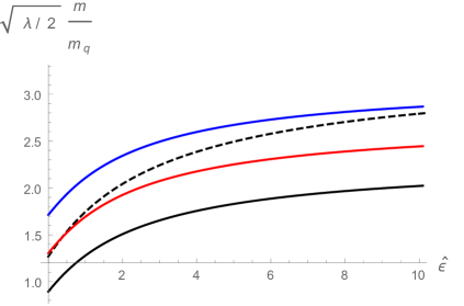
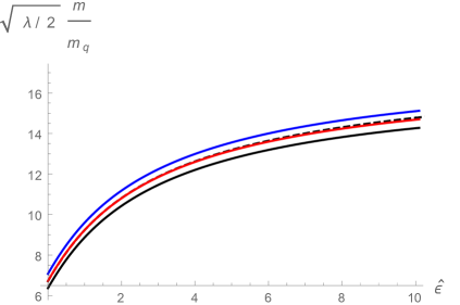
Figure 2: Meson masses in the unquenched background as a function of the flavor deformation parameter $\hat{\epsilon}$ for $\sqrt{\lambda}M/N=1$ and two values of the excitation integer: $n=0$ (left) and $n=3$ (right). The upper blue (lower black) curve corresponds to the mode $\chi_{-}$ ($\chi_{+}$). The intermediate red curve is the average of the two curves and the dashed black curve is the WKB estimate (D.20).

D.1 WKB mass spectrum

When the mass $m$ is large we can neglect the term containing the function $\Lambda$ in the fluctuation equation (D.12), and we can estimate the mass levels by using the WKB method developed in [53]. Indeed, let us consider a differential equation of the form

$$\partial_{r}\,\big{(}\,f(r)\,\partial_{r}\,R\,\big{)}\,+\,m^{2}\,h(r)\,R\,=\,0\,\,,$$ (D.13)

where $m$ is the mass parameter and $f(r)$ and $h(r)$ are two arbitrary functions that are independent of $m$. We will assume that near $r\approx r_{*}$ and $r\approx\infty$ these functions behave as:

$$f\approx f_{1}(r-r_{*})^{s_{1}}\,\,,\,\,\,\,\,\,\,\,\,\,\,\,\,\,h\approx h_{1}(r-r_{*})^{s_{2}}\,\,,\,\,\,\,\,\,\,\,\,\,\,\,\,\,{\rm as}\,\,r\to r_{*}\,\,,$$

$$f\approx f_{2}\,r^{r_{1}}\,\,,\,\,\,\,\,\,\,\,\,\,\,\,\,\,h\approx h_{2}\,r^{r_{2}}\,\,,\,\,\,\,\,\,\,\,\,\,\,\,\,\,{\rm as}\,\,r\to\infty\,\,,$$ (D.14)

where $f_{i}$, $h_{i}$, $s_{i}$, and $r_{i}$ are constants. Then, the mass levels for large quantum number $n$ can be approximately written in terms of these constants as [53]:

$$m^{2}_{WKB}\,=\,{\pi^{2}\over\xi^{2}}\,(n+1)\,\bigg{(}n\,+\,{|s_{1}-1|\over s_{2}-s_{1}+2}+{|r_{1}-1|\over r_{1}-r_{2}-2}\bigg{)}\,\,,\quad\quad\quad(n\geq 0)\,\,,$$ (D.15)

where $\xi$ is the following integral:

$$\xi\,=\,\int_{r_{*}}^{\infty}dr\,\,\sqrt{{h(r)\over f(r)}}\,\,.$$ (D.16)

In our case $f$ and $h$ are the functions:

$$f(r)\,=\,r^{2-2b}(r^{2b}-r_{*}^{2b})\,\,,$$

$$h(r)\,=\,{1\over r^{2(3-b)}}\,\Big{(}r^{2(2-b)}+(2-b)^{2}\,b^{2}\,Q^{2}\,r_{*}^{2(2-b)}\Big{)}\,\,.$$ (D.17)

The behavior of these functions at $r=r_{*}$ is characterized by the following values of the coefficients and exponents defined in (D.14):

$$f_{1}\,=\,2\,b\,r_{*}\,\,,\qquad\qquad\qquad\qquad\qquad s_{1}\,=\,1\,\,,$$

$$h_{1}\,=\,{1+(2-b)^{2}\,b^{2}\,Q^{2}\over r_{*}^{2}}\,\,,\qquad\qquad\,\,s_{2}\,=\,0\,\,.$$ (D.18)

Similarly, for the behavior at large $r$ we obtain:

$$f_{2}\,=\,1\,\,,\qquad\qquad\qquad\qquad\qquad\qquad\qquad r_{1}\,=\,2\,\,,$$

$$h_{2}\,=\,1\,\,,\qquad\qquad\qquad\qquad\qquad\qquad\qquad r_{2}\,=-2\,\,.$$ (D.19)

Therefore, the WKB mass spectrum is:

$$m_{WKB}\,=\,{\pi\over\sqrt{2}\,\xi(b,Q)}\,\sqrt{(n+1)(2n+1)}\,\,,$$ (D.20)

where $\xi(b,Q)$ is the following integral:

$$\xi(b,Q)\,\equiv\,{1\over r_{*}}\,\int_{1}^{\infty}\,{dz\over z^{2(2-b)}}\,{\sqrt{z^{2(2-b)}\,+\,(2-b)^{2}\,b^{2}\,Q^{2}}\over\sqrt{z^{2b}-1}}\,\,.$$ (D.21)

By expanding in series the square root in the numerator and integrating term by term, we can express $\xi(b,Q)$ as the following series:

$$\xi(b,Q)\,=\,-{1\over 4\,b\,r_{*}}\,\sum_{p=0}^{\infty}\,(-1)^{p}\,\big{[}(2-b)\,b\,Q\big{]}^{2p}\,{\Gamma\Big{(}p-{1\over 2}\Big{)}\over p!}\,\,{\Gamma\Big{(}{1+2p(2-b)\over 2b}\Big{)}\over\Gamma\Big{(}{1+2p(2-b)\over 2b}+{1\over 2}\Big{)}}\,\,.$$ (D.22)

Some particular values of the integral $\xi(b,Q)$ are:

$$\xi(b=1,Q)\,=\,{\pi\over 2r_{*}}\,\,F\Big{(}-{1\over 2},{1\over 2};1;-Q^{2}\,\Big{)}\,\,,$$

$$\xi(b,Q=0)\,=\,{\sqrt{\pi}\over r_{*}}\,\,{\Gamma\Big{(}{2b+1\over 2b}\Big{)}\over\Gamma\Big{(}{b+1\over 2b}\Big{)}}\,\,.$$ (D.23)

Interestingly, for $b=1$ and $Q=0$ (the unflavored model without internal flux) the WKB formula for the mass levels is exact. Moreover, for large $Q$ we can approximate $\xi(b,Q)$ as:

$$\xi(b,Q)\,\approx\,{(2-b)\,b\,Q\over r_{*}}\,\int_{1}^{\infty}\,{dz\over z^{2(2-b)}\sqrt{z^{2b}-1}}\,=\,{\sqrt{\pi}\,Q\over r_{*}}\,{(2-b)\,b\over 3-b}\,{\Gamma\Big{(}{3+b\over 2b}\Big{)}\over\Gamma\Big{(}{3\over 2b}\Big{)}}\,\,.$$ (D.24)

It follows that, for fixed quantum number $n$, the WKB mass levels for large $Q$ decrease as $1/Q$ according to the equation:

$$m_{WKB}\,\approx\,{\sqrt{\pi}\,r_{*}\over\sqrt{2}\,Q}\,{3-b\over(2-b)\,b}\,{\Gamma\Big{(}{3\over 2b}\Big{)}\over\Gamma\Big{(}{3+b\over 2b}\Big{)}}\,\sqrt{(n+1)(2n+1)}\,\,.$$ (D.25)

In Fig. 2 we compare the WKB estimates using (D.20) and the numerical results. The WKB method, however, is not valid at large values of $Q$, as it falls off the validity regime of [53]. Our numerical studies verified this expectation.

References

- [1] E. Keski-Vakkuri and P. Kraus, “Quantum Hall Effect in AdS/CFT,” JHEP 0809 (2008) 130 [arXiv:0805.4643 [hep-th]].
- [2] K. Goldstein, S. Kachru, S. Prakash and S. P. Trivedi, “Holography of Charged Dilaton Black Holes,” JHEP 1008 (2010) 078 [arXiv:0911.3586 [hep-th]].
- [3] K. Goldstein, N. Iizuka, S. Kachru, S. Prakash, S. P. Trivedi and A. Westphal, “Holography of Dyonic Dilaton Black Branes,” JHEP 1010 (2010) 027 [arXiv:1007.2490 [hep-th]].
- [4] A. Bayntun, C. P. Burgess, B. P. Dolan and S. S. Lee, “AdS/QHE: Towards a Holographic Description of Quantum Hall Experiments,” New J. Phys. 13 (2011) 035012 [arXiv:1008.1917 [hep-th]].
- [5] E. Gubankova, J. Brill, M. Cubrovic, K. Schalm, P. Schijven and J. Zaanen, “Holographic fermions in external magnetic fields,” Phys. Rev. D 84 (2011) 106003 [arXiv:1011.4051 [hep-th]].
- [6] M. Lippert, R. Meyer and A. Taliotis, “A holographic model for the fractional quantum Hall effect,” arXiv:1409.1369 [hep-th].
- [7] O. Bergman, N. Jokela, G. Lifschytz and M. Lippert, “Quantum Hall Effect in a Holographic Model,” JHEP 1010 (2010) 063 [arXiv:1003.4965 [hep-th]].
- [8] N. Jokela, M. Jarvinen and M. Lippert, “A holographic quantum Hall model at integer filling,” JHEP 1105 (2011) 101 [arXiv:1101.3329 [hep-th]].
- [9] C. Kristjansen and G. W. Semenoff, “Giant D5 Brane Holographic Hall State,” JHEP 1306 (2013) 048 [arXiv:1212.5609 [hep-th]].
- [10] O. Aharony, O. Bergman, D. L. Jafferis and J. M. Maldacena, “N=6 superconformal Chern-Simons-matter theories, M2-branes and their gravity duals,” JHEP 0810, 091 (2008) [arXiv:0806.1218 [hep-th]].
- [11] S. Hohenegger, I. Kirsch, “A Note on the holography of Chern-Simons matter theories with flavour,” JHEP 0904, 129 (2009) [arXiv:0903.1730 [hep-th]].
- [12] D. Gaiotto and D. L. Jafferis, “Notes on adding D6 branes wrapping RP**3 in AdS(4) x CP**3,” JHEP 1211 (2012) 015 [arXiv:0903.2175 [hep-th]].
- [13] Y. Hikida, W. Li, T. Takayanagi, “ABJM with Flavors and FQHE,” JHEP 0907, 065 (2009). [arXiv:0903.2194 [hep-th]].
- [14] K. Jensen, “More Holographic Berezinskii-Kosterlitz-Thouless Transitions,” Phys. Rev. D82, 046005 (2010). [arXiv:1006.3066 [hep-th]].
- [15] M. Ammon, J. Erdmenger, R. Meyer et al., “Adding Flavor to AdS(4)/CFT(3),” JHEP 0911, 125 (2009). [arXiv:0909.3845 [hep-th]].
- [16] G. Zafrir, “Embedding massive flavor in ABJM,” JHEP 1210 (2012) 056 [arXiv:1202.4295 [hep-th]].
- [17] J. Alanen, E. Keski-Vakkuri, P. Kraus and V. Suur-Uski, “AC Transport at Holographic Quantum Hall Transitions,” JHEP 0911 (2009) 014 [arXiv:0905.4538 [hep-th]].
- [18] G. Veneziano, “Some Aspects Of A Unified Approach To Gauge, Dual And Gribov Theories,” Nucl. Phys. B 117, 519 (1976).
- [19] E. Conde and A. V. Ramallo, “On the gravity dual of Chern-Simons-matter theories with unquenched flavor,” JHEP 1107 (2011) 099 [arXiv:1105.6045 [hep-th]].
- [20] N. Jokela, J. Mas, A. V. Ramallo and D. Zoakos, “Thermodynamics of the brane in Chern-Simons matter theories with flavor,” JHEP 1302 (2013) 144 [arXiv:1211.0630 [hep-th]].
- [21] C. Nunez, A. Paredes, A. V. Ramallo, “Unquenched flavor in the gauge/gravity correspondence,” Adv. High Energy Phys. 2010, 196714 (2010) [arXiv:1002.1088 [hep-th]].
- [22] Y. Bea, E. Conde, N. Jokela and A. V. Ramallo, “Unquenched massive flavors and flows in Chern-Simons matter theories,” JHEP 1312 (2013) 033 [arXiv:1309.4453 [hep-th]].
- [23] N. Jokela, A. V. Ramallo and D. Zoakos, “Magnetic catalysis in flavored ABJM,” JHEP 1402 (2014) 021 [arXiv:1311.6265 [hep-th]].
- [24] O. Aharony, O. Bergman and D. L. Jafferis, “Fractional M2-branes,” JHEP 0811 (2008) 043 [arXiv:0807.4924 [hep-th]].
- [25] G. Itsios, K. Sfetsos and D. Zoakos, “Fermionic impurities in the unquenched ABJM,” JHEP 1301, 038 (2013) [arXiv:1209.6617 [hep-th]].
- [26] A. Karch and A. O’Bannon, “Metallic AdS/CFT,” JHEP 0709 (2007) 024 [arXiv:0705.3870 [hep-th]].
- [27] G. Lifschytz and M. Lippert, “Anomalous conductivity in holographic QCD,” Phys. Rev. D 80 (2009) 066005 [arXiv:0904.4772 [hep-th]].
- [28] A. M. Dykhne and I. M. Ruzin, “Theory of the fractional quantum Hall effect: The two-phase model,” Phys. Rev. B 50, 2369 (1994).
- [29] F. Preis, A. Rebhan and A. Schmitt, “Inverse magnetic catalysis in dense holographic matter,” JHEP 1103, 033 (2011) [arXiv:1012.4785 [hep-th]].
- [30] F. Preis, A. Rebhan and A. Schmitt, “Inverse magnetic catalysis in field theory and gauge-gravity duality,” Lect. Notes Phys. 871, 51 (2013) [arXiv:1208.0536 [hep-ph]].
- [31] V. G. Filev, C. V. Johnson, R. C. Rashkov and K. S. Viswanathan, “Flavoured large N gauge theory in an external magnetic field,” JHEP 0710, 019 (2007) [hep-th/0701001].
- [32] V. G. Filev and R. C. Raskov, “Magnetic Catalysis of Chiral Symmetry Breaking. A Holographic Prospective,” Adv. High Energy Phys. 2010, 473206 (2010) [arXiv:1010.0444 [hep-th]].
- [33] V. G. Filev and D. Zoakos, “Towards Unquenched Holographic Magnetic Catalysis,” JHEP 1108, 022 (2011) [arXiv:1106.1330 [hep-th]].
- [34] J. Erdmenger, V. G. Filev and D. Zoakos, “Magnetic Catalysis with Massive Dynamical Flavours,” JHEP 1208, 004 (2012) [arXiv:1112.4807 [hep-th]].
- [35] E. Imeroni, “On deformed gauge theories and their string/M-theory duals,” JHEP 0810, 026 (2008) [arXiv:0808.1271 [hep-th]].
- [36] Y. Bea, N. Jokela and A. V. Ramallo, work in progress.
- [37] I.V. Kukushkin, J. H. Smet, V.W. Scarola, V. Umansky and K. von Klitzing, Science 324 no. 5930, 1044-1047 (2009).
- [38] N. Jokela, G. Lifschytz and M. Lippert, “Magneto-roton excitation in a holographic quantum Hall fluid,” JHEP 1102 (2011) 104 [arXiv:1012.1230 [hep-th]].
- [39] N. Jokela, M. Jarvinen and M. Lippert, “Fluctuations of a holographic quantum Hall fluid,” JHEP 1201 (2012) 072 [arXiv:1107.3836 [hep-th]].
- [40] O. Bergman, N. Jokela, G. Lifschytz and M. Lippert, “Striped instability of a holographic Fermi-like liquid,” JHEP 1110 (2011) 034 [arXiv:1106.3883 [hep-th]].
- [41] N. Jokela, M. Järvinen and M. Lippert, “Fluctuations and instabilities of a holographic metal,” JHEP 1302 (2013) 007 [arXiv:1211.1381 [hep-th]].
- [42] N. Jokela, G. Lifschytz and M. Lippert, “Magnetic effects in a holographic Fermi-like liquid,” JHEP 1205 (2012) 105 [arXiv:1204.3914 [hep-th]].
- [43] A. Ballon-Bayona, K. Peeters and M. Zamaklar, “A chiral magnetic spiral in the holographic Sakai-Sugimoto model,” JHEP 1211 (2012) 164 [arXiv:1209.1953 [hep-th]].
- [44] S. Nakamura, H. Ooguri and C. -S. Park, “Gravity Dual of Spatially Modulated Phase,” Phys. Rev. D 81 (2010) 044018 [arXiv:0911.0679 [hep-th]].
- [45] M. Rozali, D. Smyth, E. Sorkin and J. B. Stang, “Holographic Stripes,” Phys. Rev. Lett. 110 (2013) 20, 201603 [arXiv:1211.5600 [hep-th]].
- [46] B. Withers, “Black branes dual to striped phases,” Class. Quant. Grav. 30 (2013) 155025 [arXiv:1304.0129 [hep-th]].
- [47] B. Withers, “Holographic Checkerboards,” JHEP 1409 (2014) 102 [arXiv:1407.1085 [hep-th]].
- [48] N. Jokela, M. Jarvinen and M. Lippert, “Gravity dual of spin and charge density waves,” arXiv:1408.1397 [hep-th].
- [49] N. Jokela, G. Lifschytz and M. Lippert, “Holographic anyonic superfluidity,” JHEP 1310 (2013) 014 [arXiv:1307.6336 [hep-th]].
- [50] D. K. Brattan and G. Lifschytz, “Holographic plasma and anyonic fluids,” JHEP 1402 (2014) 090 [arXiv:1310.2610 [hep-th]].
- [51] N. Jokela, G. Lifschytz and M. Lippert, “Flowing holographic anyonic superfluid,” JHEP 1410 (2014) 21 [arXiv:1407.3794 [hep-th]].
- [52] K. Skenderis and M. Taylor, “Branes in AdS and pp wave space-times,” JHEP 0206 (2002) 025 [hep-th/0204054].
- [53] J. G. Russo and K. Sfetsos, “Rotating D3-branes and QCD in three dimensions”, Adv. Theor. Math. Phys. 3(1999) 131, hep-th/9901056.