Brightest X-ray clusters of galaxies in the CFHTLS wide fields:
Catalog and optical mass estimator

Abstract

The CFHTLS presents a unique data set for weak lensing studies, having high quality imaging and deep multi-band photometry. We have initiated an XMM-CFHTLS project to provide X-ray observations of the brightest X-ray selected clusters within the wide CFHTLS area. Performance of these observations and the high quality of CFHTLS data, allows us to revisit the identification of X-ray sources, introducing automated reproducible algorithms, based on the multi-color red sequence finder. We have also introduced a new optical mass proxy. We provide the calibration of the red sequence observed in the CFHT filters and compare the results with the traditional single color red sequence and photoz. We test the identification algorithm on the subset of highly significant XMM clusters and identify 100% of the sample. We find that the integrated z-band luminosity of the red sequence galaxies correlates well with the X-ray luminosity with a surprisingly small scatter of 0.20 dex. We further use the multi-color red sequence to reduce spurious detections in the full XMM and RASS data sets, resulting in catalogs of 196 and 32 clusters, respectively. We made spectroscopic follow-up observations of some of these systems with HECTOSPEC and in combination with BOSS DR9 data. We also describe the modifications needed to the source detection algorithm in order to keep high purity of extended sources in the shallow X-ray data. We also present the scaling relation between X-ray luminosity and velocity dispersion.

1 Introduction

In the past two decades the accelerating expansion of the universe has been confirmed by several experiments, such as observations of supernovae (e.g. Riess et al. 1998; Perlmutter et al. 1999) and measurements of the cosmic microwave background (e.g. Spergel et al. 2003). This acceleration is thought to be a consequence of dark energy density which, in the simplest way, can be modelled by a non-zero Einstein’s cosmological constant. Understanding the origin of the associated phenomenon of dark energy has been set among the most important tasks for understanding the formation and evolution of the Universe. Galaxy clusters play an important role in this through their sensitivity to the growth of structure. One of the first efforts in constraining cosmology with galaxy clusters was made by Borgani et al. (2001). They measured $\Omega_{M}$ using 103 galaxy clusters in the ROSAT Deep Cluster Survey (RDCS; Rosati et al. 1998) out to z$\simeq$0.85. In the subsequent study, Vikhlinin et al. (2009) obtained updated measurements of $\Omega_{M}h$, as well as the dark energy equation-of-state, $\omega_{0}$, and the amplitude of power spectrum, $\sigma_{8}$. For a review of cosmological constraints obtained using galaxy clusters in the past decade, see Weinberg et al. (2012) and Allen et al. (2011). The 2013 Planck results have revealed a tension between a combination of CMB TT fluctuation spectrum and baryonic acoustic oscillation (BAO) measurements versus galaxy cluster abundance (Planck Collaboration et al. 2013). The physical interpretation of the results in view of the non-zero neutrino mass, requires a robust understanding of the cluster scaling relations.

From an astrophysical point of view, X-ray cluster survey data provide an important definition of high-density environment, critical for studies of galaxy formation e.g. Tanaka et al. 2008; Giodini et al., 2009; Balogh et al., 2011; Giodini et al., 2012) and active galactic nuclei (AGN) (e.g. Silverman et al. 2009, Tanaka et al. 2012, Allevato et al. 2012).

The main aim of this Paper is to address the cluster identification using CFHTLS data, and to provide the cluster sample and scaling relations between optical and X-ray luminosity. The calibration between weak lensing mass and X-ray observables (luminosity and temperature) will be presented in Kettula et al. (subm.).

Optical galaxy cluster searches are often hindered by galaxy projection effects. Several algorithms have been applied to solve this problem. In addition to employing photometric methods such as red sequence identification (Gladders & Yee 2000) and MaxBCG (Annis et al. 1999; Koester et al. 2007), the detection of extended X-ray sources is often a reliable indication of galaxy clusters (Rosati et al. 2002). With the increased number of X-ray surveys in the past decade such as Chandra Deep Field North (CDFN; Bauer et al. 2002), Chandra Deep Field South (CDFS; Giacconi et al. 2002), Lockman Hole (Finoguenov et al. 2005), Cosmic Evolution Survey (COSMOS; Finoguenov et al. 2007), XMM-Large Scale Structure (XMM-LSS; Pacaud et al. 2007), Canadian Network for Observational Cosmology (CNOC2; Finoguenov et al. 2009) and Subaru-XMM Deep Field (SXDF; Finoguenov et al. 2010), X-ray astronomy introduced itself as an efficient cluster and group detection tool. In addition, X-ray properties of clusters can be used to best characterise the cluster mass, a requirement for precision cosmology work (Kravtsov et al. 2006; Nagai et al. 2007).

In this paper, we explore the use of multi-wavelength data to identify X-ray clusters within the RASS data. RASS data are both faint and unresolved, so cluster confirmation is challenging. In order to establish a reliable method, we used the highly significant extended sources, obtained through our XMM-Newton follow-up program. We start with a description of the XMM data reduction and detection of extended sources in $\S$2. In $\S$3 we present the cluster identification and validation, including spectroscopic follow-up program and velocity dispersion measurements for a subsample of clusters. $\S 4$ provides the X-ray cluster catalogs both for XMM and RASS and compares the optical luminosity and X-ray luminosity of clusters. In $\S$5 we summarise and discuss the results.

Throughout this paper, we use the AB magnitude system and consider a cosmological model with $H_{0}=72$ $\mathrm{km}$ $\mathrm{s^{-1}}$ $\mathrm{Mpc^{-1}}$, $\Omega_{\Lambda}=0.75$ and $\Omega_{M}=0.25$.

2 Data

2.1 X-ray data

The main aim of the XMM-CFHTLS program is to efficiently find massive galaxy clusters, through a series of short XMM-Newton follow-up observations of faint RASS sources (Voges et al. 1999) identified as galaxy clusters using CFHTLS imaging data. In total, 73 observations of cluster candidates have been performed, using 220ks of allocated time. At the time of scheduling XMM observations, only T0005 CFHTLS data have been publicly released, which covered 100 square degrees in partial W1 and W4 fields and the full W2 field. In order to use the mosaicing mode of XMM-Newton, we had to fulfil the re-pointing constraint of 1 degree. Given the low density of RASS sources, the number of robust clusters were rather low and for XMM snap-shot observations, we also pointed at the RASS sources identified with a photo-z galaxy overdensity. Performance of this program has allowed us to both select the adequate method for cluster identification and to perform extensive XMM studies of optically selected clusters.

The current RASS catalogs include  122 square degrees (in W1, W2, and W4), while we only have observed with XMM the clusters selected from $\sim$90 square degrees (in W2, W4, and half of W1). We would like to advise against using our data for studying the cluster abundance, as our program selectively points to clusters selected from 90 square degrees, while covering 14 square degrees. Use of our catalogs for cluster abundance studies would need to both account for RASS sensitivity and only use our RASS source list, while some of the bright XMM sources were filler optical clusters to ensure repointing constraints.

In our final catalog, we also include existing serendipitous observations, since some candidate clusters have already been previously observed with XMM. We exclude from our survey the XMM-LSS (and XXL) fields, where clusters are identified by the corresponding teams (e.g. Pacaud et al. 2007). We point out interested readers to Gozaliasl et al. (2014) where we present our catalog using the 3 square degree overlap between XMM-LSS survey and CFHTLS.

Our survey methodology is to cover a large area of the sky with short X-ray exposures. The detection of sources in such a shallow survey explores the Poisson regime, so there is a need for tailored data reduction methods. Confirming RASS sources does not require any sophisticated modelling, given that they are typically $>20\sigma$ sources, but detection of fainter serendipitous sources requires a new approach.

The procedure of Finoguenov et al. (2007, 2009) with updates described in Bielby et al. (2010) has been further revised to store the locally estimated background and exposure maps separately in order to treat the Poisson noise within the source detection program (wvdetect - Vikhlinin et al. 1998). Furthermore, we modified the ratio of thresholds for point and extended sources, setting the detection of point sources to $3.3\sigma$ and that of extended sources to $4.6\sigma$. This choice of thresholds prevents detection of point sources only on large spatial scales. The consideration of the detection effect is very general, but the ratio of thresholds is tailored for the XMM PSF and the scales of source detection we employ. In detecting the extended source, we avoid detecting the point sources, by detecting them on small scales and subtracting their flux according to PSF model, so no detection occurs on any scale anymore. The terms small and large scales are specific to XMM and refer to scales below and above 16^′′. If the source is not detected on small scales, but only detected on large scales, it would be mistaken for an extended source. An example of such a detection is a source with 3 counts in the central 16^′′ radius and 2 more counts beyond this radius. For XMM-Newton, the PSF model predicts 40% of the point source flux to occur on the scales we use for the extended source detection. The odds of not detecting the central 60% of the point source flux, while detecting the 100% of the source flux by including the outskirts are large, especially if only a few counts suffice a detection. To beat this contamination down, we need to increase the threshold for detecting the large scales, so that odds of detecting the outer 40% of the flux with a new large threshold and not detecting the central flux of the source with the original threshold are small, where small is set to be 1%, since this makes a 10% contamination to extended sources, given that point sources are 10 times more abundant. We also decrease the threshold for detecting the flux on small scales. Given the PSF shape of XMM, we find the suitable detection limits to be 3.3 $\sigma$ for the central flux and 4.6 $\sigma$ for the outskirts. We also require the significance of the flux determination associated with the detection to be above 4.6 $\sigma$. The problem described above is typical to shallow surveys, and e.g., will be important for eROSITA (Predehl et al., 2010). In deep surveys, extended source detection is background limited, which requires more counts for large scales to be detected at similar thresholds and so the flux on small scales is always detected from a point source.

The 4.6 $\sigma$ threshold XMM source list is expected to have less than 10% contamination of point sources to the extended source catalogs, which we consider acceptable, given that the highest identification rate for extended sources in deep fields is 90% (e.g. Finoguenov et al. 2010). The corresponding chance identification rate is expected to be below 2%. These estimates are conservative, since all sources in this list were identified. As in our previous work, while removing flux from point sources, we are not going through the step of cataloguing the sources, as we model the point-source contamination by convolving the wavelet images on small scales with a kernel reproducing the PSF shape on large scales.

For the provisional catalog of sources found at lower X-ray $\sigma$ ($<$ 4.6), the contamination from point sources increases to 50%. The final rate for spurious identification for such source selection is reduced due to sparse density of matching sources (optical clusters) and amounts to 10%. Given the high expected level of chance identification, this catalog is not included in the analysis of scaling relation between X-ray luminosity and integrated optical luminosity.

2.2 Optical, photometric redshift and spectroscopic data

During 2003–2009, the 3.6-m Canada-France-Hawaii Telescope (CFHT) completed a very large imaging programme known as the Canada-France-Hawaii Telescope Legacy Survey (CFHTLS) using the 2048 $\times$ 4612 pixel wide field optical imaging camera MegaCam. With a 0.185 arcsec pixel size, CFHT MegaCam gives a 0.96 degree $\times$ 0.96 degree field of view. All the observations were done in dark and grey telescope time ($\sim$ 2 300 hours). Four wide fields of this survey, with a total area amounting to 170 square degrees, were observed in $u^{\ast}$, $g^{\prime}$, $r^{\prime}$, $i^{\prime}$ and $z^{\prime}$ band down to $i^{\prime}$=24.5. In this work, we use the T0007 data release of CFHTLS and corresponding photometric redshift catalog. The photometric redshifts were computed similar to the methods of Ilbert et al. (2006); Coupon et al. (2009) . The photometric redshift catalog is limited to $i^{\prime}=24$ and according to the report of CFHTLS team, the achieved photometric redshift accuracy and outlier rates are $\sigma_{\Delta{z}\setminus{1+z}}$ $\cong$ 0.07 and $\eta\cong 13\%$ for galaxies with $22.5\leq i^{\prime}\leq 23.5$ (almost the faintest galaxies in this survey). We use optical data from three wide fields of CFHTLS: W1, W2 and W4.

Follow-up observations of clusters in W1, W2 and W4 fields were performed using Hectospec on MMT. Hectospec is a 300-fiber multi-object spectrograph with a circular field of view of 1^∘ in diameter (Fabricant et al. 2005). We used the 270 line grating, which provides a wide wavelength range (3 650 – 9 200 $\AA$) at 6.2 $\AA$ resolution. We reduced the spectra and measured redshifts using the HSRED pipeline (Cool et al. 2005). Redshifts were determined by comparing the reduced spectra with stellar, galaxy and quasar template spectra and choosing the template and redshift which minimises the $\chi^{2}$ between model and data. We then visually inspected the template fits and assigned quality flags based on the certainty of the redshift estimate.

Targets for spectroscopic follow-up were culled from the list of candidates in the XMM-CFHTLS fields and prioritised based on a combination of their X-ray flux and photometric redshift. High priority clusters (with X-ray flux $>7\times 10^{-14}$ ergs cm^-2 s^-1 and $0.15<z<0.6$) dictated the locations of the Hectospec pointings; fainter clusters or clusters beyond these redshift limits were used as fillers, and therefore only observed if they lay within $30^{\prime}$ of a high priority target. AGN candidates based on the XMM-CFHTLS point source catalogs were also used as low priority fillers. The cluster follow-up strategy used varied according to the certainty in the red sequence redshift estimate. For clusters with reliable redshifts, i.e. with high number of red sequence galaxies, we use photometric redshift catalogs to select only galaxies which lie in the photo-z slice ($dz<n\times(1+z)\times\sigma_{\mathrm{photoz}}$, where $\sigma_{\mathrm{photoz}}$ is the photometric redshift error and $n$ is an integer number between 2 and 4). The red sequence significance, $\alpha$, is a parameter that shows the overdensity of galaxies in comparison to the number of background galaxies at the cluster redshift. This parameter will be defined more accurately in section 3.1. This narrower target selection means we were able to explore the infall regions of the clusters out to larger radii. For clusters with few number of photo-z counterparts, we performed a magnitude limited survey at smaller radial distances, with the goal of identifying the optical counterparts and securing a redshift for the X-ray emission. Over the 3 fields, 32 fiber configurations were observed, mainly in W1 and W2, and secure redshifts for 6 170 objects were measured.

In performing the analysis, we have also added spectroscopic data in W1, W2 and W3 from SDSS-III survey (Aihara et al. 2011). In total, we have 13k, 3.5k and 9k spectroscopic redshifts in W1, W2 and W4.

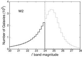
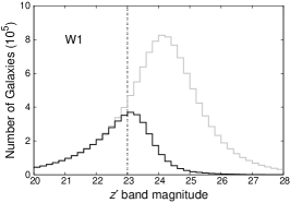
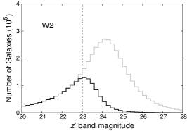
Figure 1: Distribution of the $u^{\ast}$, $g^{\prime}$, $r^{\prime}$, $i^{\prime}$ and $z^{\prime}$ magnitudes in W1 (solid line), W2 (dashed line) and W4 (dotted line) fields. The grey and black histograms belong to photometry and photometric redshift catalogs. A vertical dotted line in each plot shows defined completeness threshold magnitude below which the completeness in photoz catalog is less than 90%. Since the photometric redshift computed for galaxy $i^{\prime}<24$, the grey and black distributions are identical for galaxies in this range of magnitude.

3 Optical counterparts for X-ray sources

3.1 Red sequence method

The red sequence (Baum 1959; Bower et al. 1992; Gladders & Yee 2000) is a term defining the overdensity of early-type cluster galaxies in color-magnitude space. Usually a single color is used to find overdensities of early-type galaxies in a limited range of redshifts. This color is selected so that the 4 000 $\AA$ break is located in the bluer filter. For example, Rykoff et al. (2012) used $g^{\prime}$-$r^{\prime}$ for a redshift range between 0.1 and 0.3. However, if we select another color, such as $r^{\prime}$-$i^{\prime}$ for redshifts below 0.3, early-type galaxies (ETGs) in a cluster still produce a sequence since they have similar formation redshifts and a mostly passive evolution. While background and foreground galaxies (e.g. a late-type galaxy at higher redshift) can have similar color to the color of member ETGs, one can exclude them using other filters. This approach leads to finding member ETGs with less contamination and higher purity in selection of member galaxies, and higher sensitivity for cluster detection. On the other hand, multi-color selection of red sequence galaxies may miss some of the red sequence galaxies (lower completeness). Combination of photometric redshift and red sequence selection can also work similarly. In this Paper, we will apply the multi-color selection of red sequence galaxies to find the clusters. We will compare the relation between X-ray luminosity and integrated optical luminosity of clusters using three methods: 1) single color red sequence, 2) multi-color red sequence, and 3) combination of photoz and single color red sequence (regardless of purity and completeness for each method) to know which of them gives a better optical proxy for X-ray luminosity (or mass) of clusters.

The photometric redshifts are available in T0007 public catalog thus we only need to calibrate the red sequence method for CFHTLS wide survey. In the red sequence method, a model for describing the color of galaxies and its corresponding dispersion as a function of redshift is assumed. Then, at each redshift step, the number of red galaxies with absolute magnitude lower than a threshold is counted (using the model-predicted color value and its dispersion) and corrected for the number of background red galaxies at the same redshift. We denote the mentioned threshold on absolute magnitude as $M_{\mathrm{cut}}$. It should be adopted according to the depth of the survey in a way that the completeness is maintained in the whole redshift range. This corrected number is the cluster richness, and the redshift with the highest richness is chosen as the cluster redshift.

As we move to higher redshifts, galaxies more luminous than $M_{\mathrm{cut}}$ can still be below the completeness limit of the sample in one or more filters. Figure 1 shows the magnitude distributions of CFHTLS survey of galaxies in the W1, W2 and W4 fields in photometric catalogs in the 5 bands. We derived the photoz completeness threshold by comparison between the photoz catalog and photometry catalog. Figure 1 shows magnitude distribution for these two catalogs. We employ 0.2 magnitude bin width in calculating the distributions. We defined the completeness in photoz catalog as the magnitude above which the photoz catalog has a completeness below 90%. We display these limits with the dotted vertical lines in Figure 1. Since the photoz is computed for galaxies brighter than $i^{\prime}=24$, the completeness in other filters are almost the same for different fields. Table 1 shows the magnitude completeness limits for each field, derived this way. With the above method, we derive these completeness thresholds for photoz catalog: $u^{\ast}=24.2$, $g^{\prime}=24.2$, $r^{\prime}=24.0$, $i^{\prime}=24.0$ ,and $z^{\prime}=23.0$.

Table 1: Completeness magnitude limits for each field. Because the photometric redshift catalog has a cut at $i^{\prime}<24$, the completeness thresholds are almost the same for different fields.

filter	W1	W2	W4
$u^{\ast}$	24.2	24.2	24.4
$g^{\prime}$	24.2	24.2	24.2
$r^{\prime}$	24.0	24.0	24.0
$i^{\prime}$	24.0	24.0	24.0
$z^{\prime}$	23.0	23.0	23.0

For computing any optical quantity at different redshifts, we need to consider an identical cut on rest frame luminosity for the whole redshift range. The reason is that galaxies with similar absolute magnitude seem fainter at higher redshifts. This cut can also change the scaling relations and their scatters. For example, Rykoff et al. (2012) tested between richness and X-ray luminosity (hereafter, $L_{\mathrm{X}}$) for different $L_{\mathrm{cut}}$ from 0.1$L_{\mathrm{\ast}}$ to 0.4$L_{\mathrm{\ast}}$, showing that the richness-$L_{\mathrm{X}}$ relation of a cluster sample has the least scatter with $L_{\mathrm{cut}}=0.2L_{\mathrm{\ast}}$. In addition to minimising the scatter in the richness-$L_{\mathrm{X}}$ relation, we need to check the feasibility of selecting a given value of $L_{\mathrm{cut}}$, given the depths of the survey. Using Maraston et al. (2009) stellar population model and combining its spectral energy distribution (SED) with CFHT/MegaCam filters, we derive apparent magnitude $m_{\mathrm{\ast}}(z)$ for all filters and subsequently $k$-correction model. $m_{\mathrm{\ast}}(z)$ is the apparent magnitude of a galaxy with rest frame luminosity of $L_{\mathrm{\ast}}$ at a given redshift $z$. The computations is done by “Le Phare“ package Ilbert et al. (2006). Maraston et al. (2009) showed that their model is in agreement with color evolution of luminous red galaxies in SDSS. This model is based on a single-burst model with a solar metallicity. Similar to Rykoff et al. (2012), we adopt $L_{\mathrm{\ast}}$ = 2.25 $\times$ $10^{10}L_{\odot}$.

Figure 2 shows $m_{\mathrm{\ast}}(z)$ for all five filters derived from our model for redshifts below 1.2. Based on the magnitude completeness of the survey, we estimate the maximum redshift at which a galaxy with luminosity of 0.2, 0.4 and 1 times of $L_{\mathrm{cut}}$ can be observed in each filter. Table 2 shows the redshift limits for each $M_{\mathrm{cut}}$.

Table 2: The maximum redshift at which galaxies with luminosity of 0.2$L_{\mathrm{\ast}}$, 0.4$L_{\mathrm{\ast}}$ and 1.0$L_{\mathrm{\ast}}$ have photometric redshift in T0007 catalog.

filter	0.2$L_{\mathrm{\ast}}$	0.4$L_{\mathrm{\ast}}$	1$L_{\mathrm{\ast}}$
$u^{\ast}$	0.27	0.34	0.42
$g^{\prime}$	0.48	0.60	0.71
$r^{\prime}$	0.70	0.84	1.05
$i^{\prime}$	0.94	1.1	$>$1.2
$z^{\prime}$	1.12	$>$1.2	$>$1.2

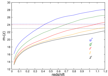
Figure 2: Characteristic magnitude $m_{\mathrm{\ast}}(z)$ for different filters as a function of redshift. Blue, green, red, yellow and black solid lines correspond to the magnitudes in $u^{\ast}$, $g^{\prime}$, $r^{\prime}$, $i^{\prime}$ and $z^{\prime}$ bands, respectively. The blue, red and black dotted lines show the completeness limits of survey for $u^{\ast}$/$g^{\prime}$, $r^{\prime}$/$i^{\prime}$, and $z^{\prime}$ filters respectively.

Figure 3: Model colors for ETGs as a function of redshift. Grey dots show the ETGs and solid lines are the average at each redshift.

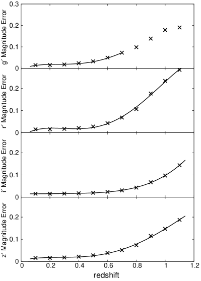
Figure 4: Magnitude errors in $g^{\prime}$, $r^{\prime}$, $i^{\prime}$ and $z^{\prime}$ band versus redshift for galaxies brighter than $m_{\mathrm{\ast(z)}}$+1. Crosses show the mean magnitude error for each redshift bin and solid lines are polynomial fits to the mean values.

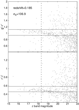
Figure 5: Color – magnitude diagrams for three clusters with high detection level in X-ray. The solid lines are upper and lower limits on the colors to encompass the bulk of red sequence galaxies. The dashed line is the $m_{\mathrm{\ast}}$+1 at the redshift of clusters.

Figure 6: Illustration of the red sequence finder using XMM cluster XCC J0224.0-0835 at a red sequence redshift of 0.28. Left panel shows the RGB image of the cluster, where $i^{\prime}$, $r^{\prime}$, and $g^{\prime}$ images are used as red, green and blue components, respectively. The X-ray flux levels are represented by the red contours and the green circles are red sequence galaxies brighter than 0.2$L_{\mathrm{\ast}}$ within 0.5 Mpc from X-ray centre. The middle panels are color magnitude diagrams, $g^{\prime}$-$r^{\prime}$ (top) and $r^{\prime}$-$i^{\prime}$ (bottom) versus $z^{\prime}$ band magnitude. Grey points are all galaxies at the redshift of the cluster, located within the radius of 0.5 Mpc from the X-ray source centre. Black dots are red galaxies brighter than 0.2$L_{\mathrm{\ast}}$ within 0.5 Mpc. In each color magnitude diagram two horizontal dotted lines are upper and lower limits of color for selecting red galaxies according to an estimate of the color scatter, described in the text. The solid vertical line shows 0.4$L_{\mathrm{\ast}}$ at the redshift of 0.3. The middle panels show the corresponding color–magnitude diagrams. The horizontal dashed lines are the lower and upper limits on the color of red sequence galaxies at a redshift of 0.3 and the solid vertical line is $L_{\mathrm{cut}}$=0.4$L_{\mathrm{\ast}}$ at the same redshift. The grey dots are all the galaxies with projected distances of 0.5 Mpc from the X-ray source centre. The black dots are the galaxies with green circles in left panel. The right panel is the variation of $\alpha$ as a function of redshift with a maximum at redshift of 0.3. The red sequence significance, $\alpha$ as a function of redshift is shown on the right panel and exhibit a maximum at a redshift of 0.3.

Given that $u^{\ast}$ band is not deep enough to cover at least half of the redshift range of 0.05 to 1.1, this filter is not used in this work. We chose the following set of redshift ranges, filters and $L_{cut}$ for red sequence algorithm:

0.05$\leq$ z $\leq$0.6 : $L_{\mathrm{cut}}$=0.4$L_{\mathrm{\ast}}$ and $g^{\prime}$,$r^{\prime}$,$i^{\prime}$

0.6$<$ z $\leq$1.1 : $L_{\mathrm{cut}}$=0.4$L_{\mathrm{\ast}}$ and $r^{\prime}$,$i^{\prime}$,$z^{\prime}$

The $r^{\prime}$ band detections become incomplete at redshifts beyond 0.84, so the identification there has to rely on a single color. As shown in Figure 2 and Table 2, $z^{\prime}$ band has the deepest imaging. We have therefore adopted $z^{\prime}$ band for the magnitude parameter in color-magnitude space. Hereinafter we use $m$ to denote the $z^{\prime}$ magnitude.

A galaxy is assumed to be on the red sequence at a redshift $z$ if:

$$|GC_{\mathrm{a-b}}-MC_{\mathrm{a-b}}(z)|<2\times\sigma_{\mathrm{a-b}}(z),$$ (1)

where $a-b$ represents a color ($g^{\prime}$-$r^{\prime}$, etc). $GC_{\mathrm{a-b}}$ and $MC_{\mathrm{a-b}}(z)$ are galaxy color and model color for red sequence galaxies at redshift $z$, respectively. $\sigma_{\mathrm{a-b}}(z)$ is the dispersion of the observed galaxy $a-b$ color around the model color. $\sigma_{\mathrm{a-b}}(z)$ is a total dispersion, given by the sum in quadrature of two other parameters, the magnitude errors and the intrinsic width of the color. In the following, we consider these two parameters in detail.

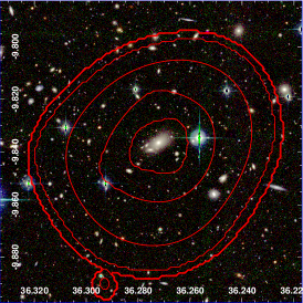
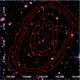
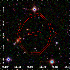
Figure 7: Examples of clusters with different visual flags. Top panels are examples of CFHTLS clusters with visual flag=1 at z=0.16, 0.46 and 0.92 (from left to right) and bottom panels are clusters with visual flag=2 at z=0.46, 0.83 and 0.55 (from left to right). We use $g^{\prime}$ band image as blue, $r^{\prime}$ – as green and $i^{\prime}$ – as red component of RGB image. The red contours show the X-ray emission. The upper clusters, from left to right, have X-ray signal significance of 31.03, 43.06, 8.77, and lower ones have 4.51, 2.15, 3.58

In order to derive the observed color evolution of red sequence galaxies, we use our spectroscopic sample of galaxies at low redshifts and a stellar population model at high redshifts. For low redshift, we select galaxies brighter than $m_{\mathrm{\ast}}(z)$+1 (or $\leq$0.4$L_{\mathrm{\ast}}$) and exclude those with AGN or star-forming classification in spectroscopic data or non-ET spectral energy distribution (SED), yielding a sample of 7 160 early-type galaxies out of the full spectroscopic redshift catalog in W1, W2, and W4. Second, we calculate the average color values and their standard deviation for these galaxies in 16 spectroscopic redshift bins from 0.05 to 0.80 with the bin size of 0.05. For each bin, we discard the galaxies with color offset from the average value exceeding two standard deviations and repeat the calculation of the mean. Figure 3 shows the $g^{\prime}$-$r^{\prime}$, $r^{\prime}$-$i^{\prime}$ and $i^{\prime}$-$z^{\prime}$ colors of ETGs and derived color model as a function of redshift (solid lines). Given that the sample of galaxies brighter than 0.4$L_{\mathrm{\ast}}$ is incomplete in g band for redshifts above 0.6, the modelling of $g^{\prime}$-$r^{\prime}$ color is limited to $z$ of 0.6.

At higher redshifts, above the redshift of 0.75, the spectroscopic sample of ETGs becomes poor, so we derive $MC_{\mathrm{a-b}}(z)$ from Maraston et al. (2009) model for early-type galaxies, the same model for $m_{\mathrm{\ast}}(z)$ model in Figure 2.

In order to determine the dispersion of the red-sequence color, $\sigma_{\mathrm{a-b}}(z)$, We assume that it has two components, an intrinsic dispersion, $\sigma_{\mathrm{a-b,int}}(z)$, and a color error, $\sigma_{\mathrm{a-b,color}}(z)$. In estimating $\sigma_{\mathrm{a-b,color}}(z)$, we selected the galaxies with photometric redshift below 1.2 and brighter than $m_{\mathrm{\ast}}(z)$+1 (similar to the original work of Gladders & Yee (2000)). Using the redshift bin width of 0.1, we determine the mean magnitude error for each band, and approximate it with the fourth order polynomials. Figure 4 illustrates the magnitude errors and the polynomial curves as functions of redshift. The total color dispersion is calculated as a sum of the color errors (derived from the magnitudes errors) and the intrinsic color dispersion in quadrature.

The red sequence is known to exhibit a tilt in the color-magnitude space due to the age-metallicity relation (Nelan et al. 2005). Since we work with both low-mass and high-z clusters, where the age-metallicity relation can be different, we prefer to consider the tilt as part of color scatter. We note that a similar approach is adopted in RedMapper (Rykoff et al., 2013). In estimating the intrinsic color dispersion, we assume that the variation of color in cluster ETGs can be modelled by a variation in metallicity. We use PEGASE.2 stellar population/galaxy formation models to estimate the intrinsic color dispersion. For the reference model, a unit solar metallicity is considered (similar to Eisenstein et al., 2001; Rykoff et al., 2012) and we model the evolution of the dispersion, by selecting the metallicity that reproduces the observed color scatter for a subsample of well observed clusters) and high number ($>10$) of spectroscopic redshifts. We model $r^{\prime}$-$i^{\prime}$ and $i^{\prime}$-$z^{\prime}$ colors between redshifts 0.05 and 1.2 and $g^{\prime}$-$r^{\prime}$ between 0.05 and 0.66. In Appendix A, it is shown that a linear evolution for intrinsic color dispersion of ETGs is a reasonable assumption especially for $g^{\prime}$-$r^{\prime}$ and $i^{\prime}$-$z^{\prime}$ colors. Thus the intrinsic color dispersions at redshifts between the two models were derived by interpolating the model points. We check the color-magnitude diagram for the training sample with different $\sigma_{\mathrm{a-b}}$ associated with different $\sigma_{\mathrm{a-b,int}}$ and realise that the metallicity of 0.75 solar is appropriate for the second model to enclose the bulk of the red sequence galaxies within two times $\sigma_{a-b}$. Figure 5 illustrates color – magnitude diagrams for three clusters at different redshifts with metallicity of 0.75 and 1 for modelling the intrinsic color dispersion. We do not optimise the width of red sequence for minimising the contamination or maximising the number of member galaxies.

The derived intrinsic dispersion of colors as functions of redshift are:

$$\sigma_{\mathrm{g^{\prime}-r^{\prime},int}}(z)=0.029+0.044\times z$$ (2)

$$\sigma_{\mathrm{r^{\prime}-i^{\prime},int}}(z)=0.011+0.046\times z$$ (3)

$$\sigma_{\mathrm{i^{\prime}-z^{\prime},int}}(z)=0.021+0.035\times z$$ (4)

.

When running the red-sequence finder, we consider a fixed physical radius for galaxy selection and vary the redshift of red sequence from 0.05 and 1.1 with a step of 0.01. At each redshift, we calculate the number of red sequence galaxies brighter than 0.4$L_{\ast}$, $N_{0.4,R}(z)$. Using 294 random areas in three optical fields we estimate the background, $NB_{0.4,R}(z)$, and its standard deviation, $\sigma_{NB}(z)$. At each redshift we compute the red sequence significance, $\alpha$, as

$$\alpha=\frac{N_{\mathrm{0.4,R}}(z)-NB_{\mathrm{0.4,R}}(z)}{\sigma_{\mathrm{NB}}(z)}.$$ (5)

The overdensity with the highest red sequence significance is adopted as the X-ray counterpart. The uncertainty in $\alpha$ is estimated by randomly changing the magnitudes of catalog galaxies according to the corresponding photometric errors.

Figure 8: Red sequence redshifts versus spectroscopic redshifts for 82 clusters with spectroscopic counterparts. The dashed line shows a 1:1 correspondence.

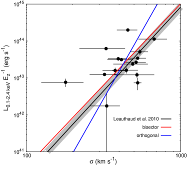
Figure 9: X-ray luminosity versus the velocity dispersion for XMM clusters with more than ten spectroscopic members from gapper estimator method. The black line shows expected $L_{\mathrm{X}}-\sigma$ from scaling relation. The grey area marks the 20% uncertainty in the mass estimate using the $L_{\mathrm{X}}-M_{200c}$ relation. The red and blue lines are fitted lines with bisector and orthogonal methods. Their equations are $log(L_{\mathrm{X}})=(31.77\pm 4.41)+(5.49\pm 2.07)log(\sigma)$ and $log(L_{\mathrm{X}})=(24.01\pm 7.37)+(10.17\pm 3.84)log(\sigma)$ respectively.

3.2 Applying the red sequence finder to identify XMM-Newton extended sources

We utilize our red sequence finder to identify the counterparts for 133 XMM-Newton extended sources in our $primary$ sample with a 4.6 $\sigma$ detection limit. We use a galaxy selection radius of 0.5 Mpc, as the centers of XMM extended sources correspond well to the cluster center (deviations are less than 15 arcseconds, George et al. 2012). Figure 6 illustrates the results of applying the red sequence on a cluster at a redshift of 0.28. After applying the red sequence finder on all the X-ray sources, we visually inspect them to compare the correspondence of a two-dimensional distribution of X-ray photons and location of galaxies, presence of secondary peaks in X-rays and optical quality of the images. The photometric and spectroscopic galaxy catalogs are fully utilised during visual inspection for optical counterparts of the X-ray sources. Obvious cluster candidates are marked with a visual flag$=1$ in the catalog. Visual flag$=2$ is assigned to X-ray sources which have low significance of the optical counterpart or concentration of galaxies almost on the edge or out of X-ray source, indicative of a confused X-ray source. Figure 7 illustrates clusters with different visual flags. It is worth mentioning that visual flag (or quality flag) has no utility in this paper and we provide it for others who will use this sample of cluster. We provide an identification to all XMM sources with flux significance above 4.6 sigma. During this inspection, we also visually checked faint sources with detection levels below 4.6, discarding the sources revealing no visual concentration of galaxies. We added 63 clusters from the lower X-ray detection threshold sample, we arrive at a sample of 196 clusters with assigned RS redshift.

81 clusters among 196 clusters have spectroscopic redshift. In defining the spectroscopic redshift, we first visually select the redshift of the brightest galaxy with spectroscopic redshift close to the red sequence redshift of a cluster and assume it as an initial redshift of a cluster. Then we select all galaxies within 0.5Mpc from X-ray centre and the sigma clipping is done within $\pm 0.005(1+z)$ around the initial redshift. Finally, the mean of spectroscopic redshifts is computed. The number of spectroscopic counterparts per cluster varies from 1 to 10 member galaxies. In Figure 8 we compare the red sequence redshift with mean of spectroscopic redshift of member galaxies. The average difference between the red sequence and spectroscopic redshift is 0.002 with a standard deviation of $0.02(1+z)$.

Figure 10: Convergence test for calculating $L_{\mathrm{S}}$. The plot shows the distribution of $L_{\mathrm{S}}$ calculated within three times of $\sigma_{a-b}(z)$ subtracted by the $L_{\mathrm{S}}$ calculated within two times of $\sigma_{a-b}(z)$. The distribution is fitted by a Gaussian with a standard deviation of 0.06 dex. The peak offset is 0.02 dex.

Figure 11: Integrated stellar luminosity in $z^{\prime}$ band versus $L_{\mathrm{X}}$ for clusters with X-ray detection level above 4.6 and $0.1<z<0.6$.

3.3 Velocity dispersion

We can also use velocity dispersion measurements as an independent confirmation for the existence of a galaxy cluster and a characteristic for the system. Such a calculation is only reliable for a high number of member galaxies (typically more than 10), though we provisionally calculate dispersions down to systems with 5 member galaxies and present them in the catalog. We limit the sample for relation between X-ray luminosity and velocity dispersion to the clusters with more than 10 member galaxies (N_σ $\leq$ 10) because of lower error in velocity dispersion measurement.

We follow the analysis of Connelly et al. (2012). In detail, we select galaxies iteratively, starting with an initial guess for the observed velocity dispersion of $\sigma(z)_{\mathrm{obs}}$=$500(1+z)$ km s^-1 as

$$\delta(z)_{\mathrm{max}}=2\frac{\sigma(z)_{\mathrm{obs}}}{c}$$ (6)

We then calculate the spatial distribution associated with $\delta(z)_{max}$:

$$\delta(r)_{\mathrm{max}}=\frac{c\delta(z)_{\mathrm{max}}}{bh_{\mathrm{71}}(z)}$$ (7)

where b=9.5 is the aspect ratio. We use the peak of the X-ray emission as the cluster center. The observed velocity dispersion, $\sigma(z)_{\mathrm{obs}}$ is then calculated for galaxies within $\delta(r)_{\mathrm{max}}$ using the $gapper$ estimator method (Wilman et al. (2005); Beers et al. (1990)), and the new value is then used to re-estimate $\delta(z)_{\mathrm{max}}$ and $\delta(r)_{\mathrm{max}}$. The procedure is repeated until convergence is achieved. The rest-frame velocity dispersion $\sigma(z)_{\mathrm{rest}}$ and intrinsic velocity dispersion $\sigma(z)_{\mathrm{int}}$ are finally given by

$$\sigma(v)_{\mathrm{rest}}=\frac{\sigma(v)_{\mathrm{obs}}}{1+z}$$ (8)

$$\langle\Delta(v)\rangle^{2}=\frac{1}{N}\sum_{\mathrm{i=1}}^{N}\Delta({v})_{i}^{2}$$ (9)

$$\sigma(v)_{\mathrm{intr}}^{2}=\sigma(v)_{\mathrm{rest}}^{2}-\langle\Delta(v)\rangle^{2}$$ (10)

where $\Delta(v)$ is the uncertainty in the spectroscopic velocity measurement. For computing velocity dispersion, we use galaxies with spectroscopic redshift error less than $3\times 10^{-4}$.

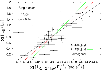
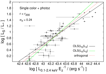
Figure 12: Integrated stellar luminosity in $z^{\prime}$ band versus $L_{\mathrm{X}}$ for clusters at $0.1<z<0.6$. The right and left panels show the results within $r_{\mathrm{200c}}$ and 1 Mpc, respectively. Upper panels use galaxy selection from multi-color red sequence, middle panels are the single-color red sequence and bottom panels belong to selection by combination of photometric redshift and single color red sequence. The solid black, solid green and dashed red lines show OLS($L_{\mathrm{S}}$—$L_{\mathrm{X}}$), OLS($L_{\mathrm{X}}$—$L_{\mathrm{S}}$) and orthogonal fits, respectively. In each panel, $\sigma_{X}$ is the scatter in $L_{\mathrm{X}}$ direction for the orthogonal fits. The fitting parameters are summarised in Table 3.

The intrinsic velocity dispersion is calculated by subtracting the contribution of redshift errors from the rest frame velocity dispersion. To assess the velocity dispersion error associated with galaxy sampling, a Jackknife method is applied (Efron, 1982) and the associated error is computed as $[\frac{N}{N-1}\sum(\delta_{i}^{2})]^{\frac{1}{2}}$, where $\delta_{i}=\sigma(v)_{\mathrm{obs}}-\sigma(v)_{\mathrm{obs,excluding\,i_{\mathrm{th}}\,member}}$, for a cluster with $N$ member galaxies. Connelly et al. (2012) showed that for calculation of velocity dispersion, applying luminosity weighted recentering can change the center up to 0.18 arcminutes but it does not change the velocity dispersion value. For more detailed description of velocity dispersion calculation, see Connelly et al. (2012) and Erfanianfar et al. (2013).

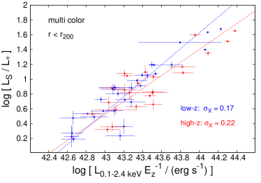
Figure 13: Stellar luminosity versus X-ray luminosity of clusters for low redshift (blue dots) and high redshift (red dots) subsample. The blue and red lines show the orthogonal fitting results for each subsample, with the parameters presented in Tab.3. The fitting parameters are summarised in Table 4

Figure 14: redMaPPer richness parameter $\lambda$ (calculated using SDSS data) versus stellar luminosity within $r_{200c}$, $L_{\mathrm{S}}$. A good correspondence between two measurements is observed.

To investigate the results of our red sequence finder and velocity dispersion calculation, let us compare ${\sigma_{\mathrm{v}}}$ to $L_{\mathrm{X}}$. Figure 9 shows the X-ray luminosity as a function of velocity dispersion for 16 XMM clusters with more than ten spectroscopic counterparts. The black line shows the expected relation between velocity dispersion and X-ray luminosity from Leauthaud et al. (2010). The grey area also shows a 20$\%$ error on mass estimate from using the $L_{\mathrm{X}}$-$M_{\mathrm{200c}}$ relation (Allevato et al., 2012). We do not account for the intrinsic scatter between velocity dispersion and $M_{200c}$. The blue and red lines are fitted lines using bisector and orthogonal fitting methods (Akritas & Bershady (1996)). The bisector method minimises the square distance independently in X and Y directions. The orthogonal method minimises the squared orthogonal distances. The result of bisector fitting method is very close to the relation, expected from the weak lensing calibration. While most of the clusters are close to the predicted relation, three of them have significantly larger $L_{\mathrm{X}}$ than the values of $L_{\mathrm{X}}$ predicted by the scaling relation. Since this offset is about one order of magnitude in $L_{\mathrm{X}}$, a significant contribution of unresolved X-ray point sources can be ruled out. Among these three clusters, two less luminous ones have N_σ of 12 and 13 and the more luminous one has 20. As discussed in Ruel et al. (2013), the low number of spectroscopic members can be a reason for these deviations. The compatibility between our ${\sigma_{\mathrm{v}}}$–$L_{\mathrm{X}}$ relation and the scaling relation of Leauthaud et al. (2010) indicates that although Leauthaud et al. (2010) relation was derived using a sample of clusters mostly with $L_{\mathrm{X}}<10^{43}ergs^{-1}$, it is still reliable for mass estimation of more luminous clusters.

Table 3: Fitting parameters of $log(L_{\mathrm{X}})$–$log(L_{\mathrm{S}})$ relation. Col.(1) indicates the type of selection of red galaxies; col.(2) is the radius within which $L_{\mathrm{X}}$ is calculated. The fitting procedure is listed in col.(3). The cols. (4–5) present the intercept and slope of fittings respectively. The scatter in log$L_{\mathrm{X}}$ and log$L_{\mathrm{S}}$ direction are in cols. (6–7).

red sequence	radius	Fitting	intercept	slope	$L_{\mathrm{X}}$ scatter	$L_{\mathrm{S}}$ scatter
					dex	dex
		OLS($L_{\mathrm{S}}|L_{\mathrm{X}}$)	-38.97$\pm$2.97	0.92$\pm$0.07	0.21	0.19
multi-color	$r_{\mathrm{200c}}$	OLS($L_{\mathrm{X}}|L_{\mathrm{S}}$)	-44.33$\pm$3.21	1.04$\pm$0.07	0.20	0.21
		orthogonal	-41.51$\pm$3.11	0.98$\pm$0.07	0.20	0.20
		OLS($L_{\mathrm{S}}|L_{\mathrm{X}}$)	-40.46$\pm$5.13	0.95$\pm$0.12	0.28	0.27
single color	$r_{\mathrm{200c}}$	OLS($L_{\mathrm{X}}|L_{\mathrm{S}}$)	-54.12$\pm$5.39	1.27$\pm$0.12	0.25	0.32
		orthogonal	-47.50$\pm$5.03	1.12$\pm$0.12	0.26	0.29
		OLS($L_{\mathrm{S}}|L_{\mathrm{X}}$)	-37.47$\pm$4.19	0.88$\pm$0.10	0.26	0.23
single color + photoz	$r_{\mathrm{200c}}$	OLS($L_{\mathrm{X}}|L_{\mathrm{S}}$)	-48.82$\pm$4.46	1.15$\pm$0.10	0.23	0.27
		orthogonal	-42.82$\pm$3.57	1.01$\pm$0.08	0.24	0.24
		OLS($L_{\mathrm{S}}|L_{\mathrm{X}}$)	-31.71$\pm$2.95	0.75$\pm$0.07	0.28	0.21
multi-color	1 Mpc	OLS($L_{\mathrm{X}}|L_{\mathrm{S}}$)	-42.15$\pm$4.33	0.99$\pm$0.10	0.25	0.24
		orthogonal	-35.77$\pm$3.58	0.85$\pm$0.08	0.26	0.22
		OLS($L_{\mathrm{S}}|L_{\mathrm{X}}$)	-31.12$\pm$4.35	0.74$\pm$0.10	0.37	0.27
single color	1 Mpc	OLS($L_{\mathrm{X}}|L_{\mathrm{S}}$)	-52.18$\pm$7.32	1.23$\pm$0.17	0.29	0.36
		orthogonal	-39.75$\pm$5.99	0.94$\pm$0.14	0.31	0.29
		OLS($L_{\mathrm{S}}|L_{\mathrm{X}}$)	-37.47$\pm$4.19	0.88$\pm$0.10	0.32	0.26
single color + photoz	1 Mpc	OLS($L_{\mathrm{X}}|L_{\mathrm{S}}$)	-48.82$\pm$4.46	1.15$\pm$0.10	0.27	0.31
		orthogonal	-42.82$\pm$3.57	1.01$\pm$0.08	0.28	0.27

Table 4: Fitting parameters of $log(L_{\mathrm{X}})$–$log(L_{\mathrm{S}})$ relation for low and high redshift subsamples. Stellar luminosity computed using multi-color selection. Col.(1) indicates redshift ranges of redshift ranges; col.(2) is the radius within which $L_{\mathrm{X}}$ is calculated. The fitting procedure is listed in col.(3). The cols. (4–5) present the intercept and slope of fittings respectively. The scatter in log$L_{\mathrm{X}}$ and log$L_{\mathrm{S}}$ direction are in cols. (6–7).

redshift	radius	Fitting	intercept	slope	$L_{\mathrm{X}}$ scatter	$L_{\mathrm{S}}$ scatter
					dex	dex
		OLS($L_{\mathrm{S}}|L_{\mathrm{X}}$)	-44.56$\pm$4.10	1.05$\pm$0.09	0.17	0.18
0.1 $<$ z $<$ 0.3	$r_{\mathrm{200c}}$	OLS($L_{\mathrm{X}}|L_{\mathrm{S}}$)	-46.69$\pm$3.10	1.10$\pm$0.09	0.17	0.19
		orthogonal	-45.69$\pm$3.89	1.08$\pm$0.09	0.17	0.18
		OLS($L_{\mathrm{S}}|L_{\mathrm{X}}$)	-33.61$\pm$3.59	0.79$\pm$0.08	0.23	0.19
0.3 $<$ z $<$ 0.6	$r_{\mathrm{200c}}$	OLS($L_{\mathrm{X}}|L_{\mathrm{S}}$)	-42.49$\pm$5.13	0.10$\pm$0.12	0.21	0.21
		orthogonal	-37.27$\pm$4.22	0.88$\pm$0.10	0.22	0.19
		OLS($L_{\mathrm{S}}|L_{\mathrm{X}}$)	-35.54$\pm$3.81	0.84$\pm$0.09	0.24	0.21
0.1 $<$ z $<$ 0.3	1 Mpc	OLS($L_{\mathrm{X}}|L_{\mathrm{S}}$)	-43.27$\pm$5.65	1.02$\pm$0.13	0.23	0.23
		orthogonal	-38.91$\pm$4.38	0.92$\pm$0.10	0.23	0.21
		OLS($L_{\mathrm{S}}|L_{\mathrm{X}}$)	-29.42$\pm$4.14	0.69$\pm$0.10	0.29	0.20
0.3 $<$ z $<$ 0.6	1 Mpc	OLS($L_{\mathrm{X}}|L_{\mathrm{S}}$)	-42.79$\pm$6.85	1.01$\pm$0.16	0.24	0.25
		orthogonal	-34.25$\pm$5.50	0.81$\pm$0.13	0.26	0.21

3.4 Stellar luminosity as a $L_{\mathrm{X}}$ estimator

We calculate the integrated $z^{\prime}$-band luminosity, $L_{\mathrm{S}}$, of red sequence galaxies (brighter than $0.4L_{\mathrm{\ast}}$) within $r_{\mathrm{200c}}$, for clusters in the redshift range of 0.1$<$z$<$0.6 and the X-ray detection threshold above 4.6. The $r_{\mathrm{200c}}$ is also calculated from $M_{\mathrm{200c}}$ (see section 4). The luminosity of red sequence galaxies are added to each other and subtracted by background luminosity at the same redshift. The background is the mean of integrated luminosity of the red sequence galaxies at random points in sky and within the similar radius. In §3.1, we mentioned that we define the width of the red sequence to enclose the bulk of bright red sequence galaxies. Here we show that the adopted width does not affect the measured stellar luminosity of the clusters. For this purpose, we increase the widths of all colors in the red sequence selection to three times the $\sigma_{a-b}(z)$ (1.5 times the previous width) and re-computed the stellar luminosity. The background computation was also repeated for changing the width of red sequence. Figure 10 illustrates the variation of $L_{\mathrm{S}}$ after increasing the width of red sequence by 50$\%$. The change in $L_{\mathrm{S}}$ is 0.02 dex with a standard deviation of 0.06 dex. We conclude that the obtained $L_{\mathrm{S}}$ values have converged.

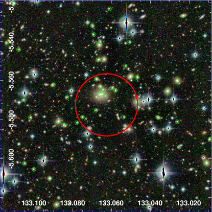
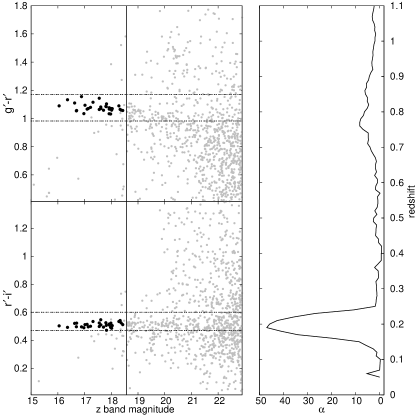
Figure 15: As in Figure 6 but for a RASS cluster at the redshift of 0.19. The position of the RASS source is shown by a large red circle with a radius of one arcminute.

Figure 16: Left: Red sequence significance, $\alpha$, versus redshift for RASS X-ray sources. Right: Red sequence significance, $\alpha$, versus offset between optical and X-ray cluster centers. Red circles mark the RASS X-ray sources and black circles are random sources in CFHTLS. A blue dashed line shows the criteria for selection of clusters among the RASS sources. The right-hand panel shows $\alpha$ versus the redshift for the RASS and random sources. In this panel, blue circles are the RASS clusters.

Figure 17: X-ray mass (top) and X-ray luminosity (bottom) as functions of redshift. Black dots and open circles show XMM-CFHTLS and COSMOS X-ray selected galaxy clusters. The errors are calculated with statistical errors in the X-ray flux measurements. 16 XMM clusters in common to RASS clusters are marked as squares. In both panels, the solid curves show the detection limits in luminosity- and mass-redshift spaces corresponding to X-ray flux limit of $2\times 10^{-13}erg$ $cm^{-2}s^{-1}$.

Figure 18: RASS X-ray flux versus XMM-Newton X-ray flux for 16 clusters in overlap between the RASS and XMM cluster samples. A solid curve shows the the prediction for Malmquist bias in RASS flux measurement.

In some cases, bright stars affect the photometry. We discard the affected clusters from determination of $L_{\mathrm{X}}$. Figure 11 illustrates the relation between $L_{\mathrm{S}}$ and $L_{\mathrm{X}}$ for the sample of clusters in the redshift range of 0.1$<$z$<$0.6 and the X-ray detection threshold above 4.6. There is a strong correlation between $log(L_{\mathrm{S}})$ and $log(L_{\mathrm{X}})$ for the bulk of the sample. The Spearman test coefficient for this relation is 0.640 with the zero value for the probability of null hypothesis of null correlation between two quantities.

The good relation between $L_{\mathrm{S}}$ and $L_{\mathrm{X}}$ is a motivation for using $L_{\mathrm{S}}$ as an estimator for $L_{\mathrm{X}}$ and, consequently, the cluster mass. For this purpose, besides of $L_{\mathrm{S}}$ within $r_{\mathrm{200c}}$, we also measure the $L_{\mathrm{S}}$ within 1 Mpc from the X-ray centre. Figure 12 illustrates the relation between $L_{\mathrm{S}}$ and $L_{\mathrm{X}}$ for the sample of clusters. The upper left and upper right panels show the $L_{\mathrm{S}}$ computed within $r_{\mathrm{200c}}$ and 1 Mpc, respectively. The later is useful in the situations when the measurement of the virial radius is not possible or noisy. In Figure 12, the lines show the power-law fits to the relation. The procedures of Akritas & Bershady (1996) ordinary least square (OLS) and bi-variate correlated errors and intrinsic scatter (BCES) estimators are used to produce the fits. The ordinary least square estimators in $L_{\mathrm{X}}$ direction (OLS($L_{\mathrm{X}}$—$L_{\mathrm{S}}$)) and $L_{\mathrm{S}}$ direction (OLS($L_{\mathrm{S}}$—$L_{\mathrm{X}}$)) are shown as black and green solid curves, respectively. The red dashed lines are the results of BCES orthogonal fitting method, which minimises the squared orthogonal distances. The parameters of the plotted relations are listed in Table 3.

For comparison to the multi-color red sequence, we compute the $L_{\mathrm{S}}$ with a single-color selection of red sequence galaxies ($g^{\prime}-r^{\prime}$ for 0.05$\leq$ z $\leq$0.4 and $r^{\prime}-i^{\prime}$ for 0.4$<$ z $\leq$0.6). We also compute the $L_{\mathrm{S}}$ with a combination of photometric redshift and single-color selection of red sequence galaxies. In this method, $L_{\mathrm{S}}$ is computed for galaxies that satisfy both conditions of photoz range and single-color. We need to adopt a suitable redshift range for photoz selection. A suitable redshift range is the sum in quadrature of two redshift errors, uncertainty in measurement of cluster redshift and errors in photometric redshift of galaxies. In $\S$ 3.2, we show that our red sequence technique has an uncertainty of $0.02(1+z)$ in cluster redshift measurement. The accuracy in photometric redshift varies with galaxy magnitude. We assume the worst photoz accuracy which belongs to the galaxies with brightness of $m_{\mathrm{\ast}}$+1 at redshift 0.6. According to the Figure 8, the z-band magnitude of such galaxy is $21.1$. We compute the photometric redshift error for galaxies with z-band magnitude of between 20.6 and 21.1. For 886 galaxies with such magnitude and with spectroscopic redshift in the three fields of CFHTLS, the photometric redshift error is $0.031(1+z)$. For selection of member galaxies, we adopt the redshift interval of $\pm 0.07(1+z)$ around the mean redshift of the cluster.

The best method (among multi-color, single-color and single-color-photoz) is sought to provide the lowest scatter versus $L_{\mathrm{X}}$. The results are compared in Figure 12, using $r_{\mathrm{200c}}$ and 1 Mpc as an extraction radius. The middle and bottom panels of Figure 12 show the relation between the cluster X-ray luminosity versus $L_{\mathrm{S}}$ computed using the single color and single-color-photoz methods, respectively. These relations are fitted with power-law models, and the results of fitting are shown in Table 3.

For all $L_{\mathrm{X}}-L_{\mathrm{S}}$ scaling relations the scatter for the multi-color red sequence finder is smaller than or equal to the single-color and single-color-photoz values, independent of the selection radius and the fitting method. For example, for $L_{\mathrm{S}}$ computed with $r_{200c}$, the orthogonal relation has a scatter of 0.20, 0.29, and 0.24 dex in $L_{\mathrm{X}}$ for multi-color, single color, and a combination of single color and photoz respectively. The reduction of scatter is even more significant in the case of a fixed 1 Mpc radius. For instance, the orthogonal scatter is 0.26 dex in $L_{\mathrm{X}}$ for the multi-color, 0.31 dex for the single-color and 0.28 dex for the combination of single-color and photoz. Our results on the tight relation between the $L_{\mathrm{S}}$ and other mass proxies, such as $L_{\mathrm{X}}$ are in line with the low redshift studies of Rykoff et al. (2012) at 0.1$<$z$<$0.3 and Andreon (2012) for z$<$0.14.

In Figure 13 we consider the redshift evolution of the $L_{\mathrm{S}}$–$L_{\mathrm{X}}$ relation. Using two subsamples with 0.1$<$z$<$0.3 and 0.3$<$z$<$0.6, we find a difference in the relation to X-ray luminosity ($L_{\mathrm{X}}$ $>$ 42.5 ergs s^-1). The low redshift relation is within the errors of high redshift relation. The parameters of the relation are presented in Table 4. The scatter in $L_{\mathrm{X}}$ reduces down to 0.17dex for low redshift sample.

To compare our red sequence finder to other work, Figure 14 shows $L_{\mathrm{X}}$ versus richness parameter $\lambda$ used in redMaPPer (next generation of MaxBCG method, Rykoff et al. 2013), designed to find clusters in SDSS data. Briefly, redMaPPer applies a red sequence model and assumes radial and luminosity filters to calculate the probability that a given galaxy belongs to a cluster. The parameter $\lambda$ is the sum of mentioned probabilities. There are 10 RASS clusters in overlap between SDSS and the CFHTLS fields. The large errors in $\lambda$ for a few clusters are caused by the shallow depths of SDSS data. Rozo & Rykoff (2014) reported a scatter of 0.23 dex in X-ray temperature at fixed $\lambda$. Figure 14 shows that $L_{\mathrm{S}}$ and $\lambda$ correlate.

3.5 Applying the red sequence finder to identify RASS sources

Performance of our XMM program was based on the identification of RASS sources as galaxy clusters. This lead to the development and verification of the source identification methods reported above. It allows us to present a consistent identification of RASS sources using the same method, which allows us to both characterise the target selection, and to report the clusters which we have not observed, since we include the full CFHTLS dataset in this analysis, covering 180 square degrees.

We apply the red sequence finder to identify clusters associated with 245 RASS sources within the three CFHTLS fields in our study. According to the $log(N)-log(S)$ relation, clusters make up only 10% of X-ray sources (Finoguenov et al. 2007; Cappelluti et al. 2007), making cluster identification difficult using unresolved X-ray sources in RASS data. The radius for galaxy selection has been set to 0.5 Mpc at each redshift plus two arcminutes to account for the survey PSF of RASS. After finding the red member galaxies, we derive the $z^{\prime}$-band luminosity weighted center for each cluster candidate, which then defines the distance between the optical counterpart and the X-ray source position (hereafter Opt–X-ray distance). Figure 15 shows the red sequence finder results for a cluster at a redshift of 0.19.

In order to distinguish between X-ray sources associated by clusters and other X-ray sources, we used Opt–X-ray distance and $\alpha$ parameters. With a comparison between properties of RASS sources and random sources, we try to find X-ray clusters among RASS sources. We similarly apply the red sequence finder on 300 random sources in CFHTLS fields. Figure 16 shows $\alpha$ parameter versus Opt–X-ray and redshift for RASS and random sources. The red circles represent the 245 RASS sources and black circles are random points in CFHTLS fields. While only a handful of random sources can have high $\alpha$ values (15 or more) and low Opt–X-ray distance, tens of RASS sources achieve such values. This suggests that a combination of $\alpha$ and Opt–X-ray distance can discriminate between clusters and other sources of X-ray emission. We select the X-ray clusters by cuts of $13<\alpha$ and Opt–X-ray distance less than 2.5 arcminutes. The left panel in Figure 16 illustrates the cuts in blue dashed line. Nine random sources and 32 RASS X-ray sources located in selection region that shows the purity ($\sim$ 80 %) in selected sample of X-ray clusters with this method. We will show in $\S$4 that by adopted criteria, we can detected all XMM clusters with X-ray flux above the RASS X-ray detection threshold. By increasing $\alpha$ value one can achieve a purer sample. For instance, 20 RASS sources have $20<\alpha$ but only one random source has such high $20<\alpha$ value.

4 RASS-CFHTLS and XMM-CFHTLS catalogs of X-ray selected clusters

In this section, we present the RASS and XMM (X-ray) selected cluster catalogs. The first catalog, Table 5, belongs to the 196 XMM clusters. The first 133 lines in Table 5 belong to the sample with X-ray detection threshold above 4.6 sigma and the last 63 lines are those with lower detection threshold. Column 1 in Table 5 shows the cluster ID for the XMM-CFHTLS sample with the first digit referring to the CFHTLS wide field (1,2 or 4). Columns 2 and 3 are respectively R.A. and Dec. of the X-ray source centers. Columns 4 and 5 are the red sequence redshift and red sequence significance, $\alpha$, of the clusters. Column 6 lists cluster flux and one sigma error in flux corresponding to the 0.5–2 keV band in units of 10^-14 ergs cm^-2 s^-1. Column 7 reports the rest-frame X-ray luminosity, $L_{\mathrm{X}}$, in the 0.1–2.4 keV band. The total mass $M_{\mathrm{200c}}$, estimated from the X-ray luminosity using the Lx–M scaling relation and its evolution from Leauthaud et al. (2010), is given in column 8. Column 9 lists corresponding radius, $r_{\mathrm{200c}}$, in arcminutes. Spectroscopic redshifts of the clusters are provided in column 10. For clusters with a spectroscopic redshift in this column, $M_{\mathrm{200c}}$, and, $r_{\mathrm{200c}}$ are computed using spectroscopic redshift. Column 11 reports the visual flag described in Sect. 3.2. Velocity dispersion and number of spectroscopic members (both described in Sect. 3.3) for clusters having more than five spectroscopic members are given in columns 12 and 13, respectively.

The RASS-CFHTLS cluster catalog is listed in Table 6. This catalog includes 32 clusters with selection shown in the left-hand panel of Figure 16. Column 1 is the cluster ID. The coordinates (RA and DEC, Equinox J2000) of the clusters are given in columns 2 and 3. The red sequence redshift and significance ($\alpha$) are listed in column 4 and 5. The position of the optical center is reported in columns 6 and 7. Columns 8 and 9 report ROSAT X-ray flux and luminosity in units of $10^{-13}$ erg s^-1 cm^-2 and $10^{42}$ erg s^-1 respectively. The spectroscopic redshifts which were also verified visually are given in column 10. The columns 11 and 12 present the velocity dispersion and the number of spectroscopic member galaxies from Sect. 3.3. Based on the derived relation between $L_{\mathrm{X}}$ and $L_{\mathrm{S}}$, we estimate the $L_{\mathrm{X}}(L_{\mathrm{S}})$ for 32 RASS clusters. We measured $L_{\mathrm{S}}$ within 1 Mpc from the optical center of clusters (column 6 and 7 in table 6). The estimated cluster $L_{\mathrm{X}}$ using orthogonal fitting result (in Table 4 with 0.23 and 0.26 dex scatter in X-ray luminosity for low and high redshifts respectively) are listed in column 13 of table 6.

The inferred mass and X-ray luminosity of the XMM clusters as a function of redshift are illustrated in Figure 17. We mark 16 XMM clusters in common to RASS clusters as squares. This sub-sample of RASS clusters stems from our targeted follow-up observations of RASS clusters found inside the part of CFHTLS survey publicly released in T0005 and presents an effective search for massive clusters in the area of 90 square degrees. The two curves in Figure 17 show the detection boundary related to $2\times 10^{-13}erg$ $cm^{-2}s^{-1}$ in X-ray flux. This flux is associated with a detection limit over 85% of the survey area. All XMM clusters more luminous or massive than these two curves are also identified as RASS clusters using adopted criteria for selection of clusters among RASS sources (see $\S$ 3.5). The mass (and luminosity) detection limit, shown with a curve in Figure 17, also implies that only extreme clusters ($\sim 10^{15}M_{\odot}$) at redshift $\sim 1$ are detectable in RASS data.

We added COSMOS X-ray selected galaxy clusters (Finoguenov et al. 2007, George et al. 2011) to the plots, to show the difference in the cluster sample. At a fixed redshift, the typical mass (and luminosity) of XMM-CFHTLS clusters are an order of magnitude more massive (and more luminous) in comparison with a typical group in deep surveys such as COSMOS. For example, at the redshift range of $0.2\leq z\leq 0.3$, the median of the $M_{\mathrm{200c}}$ of XMM-CFHTLS and COSMOS clusters are respectively 1.1$\times 10^{14}$ M_⊙ and 2.6$\times 10^{13}$ M_⊙. This difference between the mean total mass (and luminosity) is even larger between COSMOS and RASS-CFHTLS clusters.

A comparison of the X-ray fluxes from RASS and XMM is presented in Figure 18. At low flux levels, the RASS flux estimates are subject to the Malmquist bias, as shown by a model curve. We also report that the mean of distances between the centre of RASS and XMM X-ray emissions is 0.6 arcminutes for 16 clusters in overlap between RASS and XMM samples.

5 Summary

We have presented the results of an X-ray search for bright clusters in the CFHTLS fields. In this work we presented the cluster identification in RASS and XMM data. We developed a method for identifying clusters at the limits of RASS data, reaching flux levels of $2\times 10^{-13}$ erg cm^-2 s^-1, with the help of deep photometric data, such as that of CFHTLS.

We have described a multi-color red sequence finder and calibrated it for CFHTLS $u^{\ast}g^{\prime}r^{\prime}i^{\prime}z^{\prime}$ filters and the redshift below 1.1. The spectroscopic follow-up was done using the Hectospec spectrograph on MMT, with higher priority for clusters with high X-ray flux. To increase the efficiency of spectroscopic follow-up, target galaxies were selected within a range of photometric redshift around the red sequence redshift of clusters. In this work we also used SDSS spectroscopic data in the CFHTLS wide fields. We applied our red sequence finder on RASS and XMM-Newton X-ray sources in the W1, W2, and W4 CFHTLS fields. In total, we identified 32 clusters associated with RASS sources and 196 clusters among XMM X-ray sources, with a 100% identification rate achieved for the high-significance XMM sample. We computed the X-ray luminosity and mass from the X-ray flux and the scaling relations from the literature. In comparison to other XMM samples, the clusters in our sample are typically of $\sim$ $10^{14}$ M_⊙ masses, while e.g., COSMOS X-ray selected groups are of an order of magnitude lower mass. We calculated the velocity dispersions with an iterative gapper method and derive the scaling relation between velocity dispersion and X-ray luminosity of clusters.

We also explored a correlation of integrated optical luminosity and X-ray luminosity. We showed that multi-color red sequence reduces the scatter in relation with X-ray luminosity. This set of optical methods for cluster finding are particularly useful for providing large samples of X-ray luminous (or massive) clusters (especially for cosmological studies) using shallow X-ray data and wide optical surveys. First, by applying the red sequence finder and maximising $\alpha$, we can extract a pure sample of clusters out of a list of X-ray sources. Second, by measuring the optical luminosity of clusters within an appropriate fixed radius we can estimate the cluster total mass, allowing an efficient separation of high X-ray luminous (high-mass) clusters for further studies.

Table 5: Catalog of XMM-CFHTLS X-ray Selected Galaxy Clusters

ID	RA	DEC	R.S. z	$\alpha$	X-ray Flux	$L_{X}$	$M_{200c}$	$r_{200c}$	specz	visual flag	$\sigma(v)$	$N_{\sigma}$
XMM-CFHTLS	(degrees)	(degrees)			$10^{-14}erg$ $cm^{-2}s^{-1}$	$10^{42}erg$ $s^{-1}$	$10^{13}M_{\odot}$	arcmin			($kms^{-1})$
(1)	(2)	(3)	(4)	(5)	(6)	(7)	(8)	(9)	(10)	(11)	(12)	(13)
XCC J0210.4-0343	32.6184	-3.7202	0.45	0.86$\pm$0.92	3.39$\pm$0.54	37.08$\pm$5.96	14.42$\pm$1.44	2.73	0.4417	1	-	1
XCC J0211.0-0905	32.7665	-9.0977	0.45	0.86$\pm$1.45	4.28$\pm$1.70	48.05$\pm$19.15	16.90$\pm$4.04	2.838	-	2	-	-
XCC J0211.2-0343	32.8079	-3.7226	0.78	20.48$\pm$2.30	7.52$\pm$1.04	271.79$\pm$37.86	37.77$\pm$3.28	2.526	-	1	-	-
XCC J0211.3-0927	32.8338	-9.4567	0.71	1.38$\pm$1.17	2.73$\pm$1.05	88.06$\pm$33.76	19.60$\pm$4.52	2.16	-	2	-	-
XCC J0211.4-0920	32.8551	-9.3366	0.84	1.20$\pm$0.59	3.83$\pm$1.95	173.23$\pm$88.38	26.77$\pm$8.08	2.148	-	2	-	-
XCC J0211.5-0939	32.8894	-9.6606	0.51	4.82$\pm$1.30	3.03$\pm$1.41	40.33$\pm$18.78	14.70$\pm$4.07	2.586	0.4801	2	-	1
XCC J0212.2-0852	33.0716	-8.8752	0.09	1.93$\pm$1.72	7.93$\pm$3.20	2.62$\pm$1.05	3.52$\pm$0.85	6.318	0.094	2	-	3
XCC J0213.4-0813	33.37	-8.2204	0.26	2.76$\pm$1.02	6.96$\pm$1.82	18.04$\pm$4.72	10.86$\pm$1.74	4.08	0.2358	1	446$\pm$84	12
XCC J0213.6-0552	33.4141	-5.8707	1.1	4.40$\pm$0.75	2.14$\pm$0.91	186.85$\pm$80.19	22.11$\pm$5.67	1.704	-	2	-	-
XCC J0214.1-0630	33.545	-6.516	0.88	1.03$\pm$0.93	1.24$\pm$0.47	70.62$\pm$26.81	14.52$\pm$3.32	1.698	-	2	-	-
XCC J0214.4-0627	33.6064	-6.4605	0.25	13.80$\pm$1.26	27.67$\pm$49.35	69.48$\pm$123.92	25.73$\pm$23.81	5.424	0.2366	1	329$\pm$108	12
XCC J0215.6-0702	33.9113	-7.0478	1.02	-1.78$\pm$0.33	1.33$\pm$0.43	104.43$\pm$33.88	16.39$\pm$3.22	1.614	-	2	-	-
XCC J0215.7-0654	33.9274	-6.9051	0.23	2.76$\pm$1.02	5.79$\pm$1.48	17.83$\pm$4.56	10.62$\pm$1.66	3.804	0.2544	1	377$\pm$65	10
XCC J0216.1-0935	34.0291	-9.5885	0.62	21.55$\pm$1.39	5.95$\pm$0.86	121.63$\pm$17.66	26.81$\pm$2.43	2.706	0.5955	1	-	4
XCC J0216.5-0658	34.1416	-6.9691	1.1	-2.59$\pm$0.25	1.26$\pm$0.54	118.05$\pm$50.52	16.48$\pm$4.22	1.542	-	2	-	-
XCC J0216.7-0934	34.1938	-9.5702	0.94	7.82$\pm$0.69	1.58$\pm$0.51	101.42$\pm$33.12	17.31$\pm$3.43	1.728	-	2	-	-
XCC J0217.5-0655	34.3779	-6.9236	1.01	0.30$\pm$0.34	1.38$\pm$0.78	106.01$\pm$60.14	16.70$\pm$5.56	1.632	-	2	-	-
XCC J0217.5-0936	34.3788	-9.6136	0.39	3.87$\pm$1.31	1.70$\pm$0.60	14.43$\pm$5.15	8.25$\pm$1.78	2.49	-	2	-	-
XCC J0217.5-0927	34.3874	-9.462	0.46	5.85$\pm$3.15	6.80$\pm$2.38	120.11$\pm$42.06	27.48$\pm$5.82	2.85	0.56	1	-	2
XCC J0217.8-0641	34.4574	-6.689	1.04	-0.03$\pm$0.73	2.13$\pm$0.99	165.26$\pm$76.94	21.59$\pm$5.98	1.746	-	2	-	-
XCC J0217.9-0648	34.4871	-6.8068	0.84	-0.79$\pm$0.51	1.28$\pm$0.51	64.99$\pm$26.26	14.29$\pm$3.46	1.74	-	2	-	-
XCC J0218.0-0937	34.5029	-9.6256	0.15	1.79$\pm$1.07	4.46$\pm$0.89	4.75$\pm$0.95	4.91$\pm$0.61	4.374	0.1598	1	232$\pm$73	9
XCC J0218.3-0942	34.5814	-9.7028	0.45	3.86$\pm$3.18	2.62$\pm$0.73	21.93$\pm$6.11	10.78$\pm$1.83	2.718	0.3908	1	-	1
XCC J0219.6-0759	34.9039	-7.9882	0.86	1.13$\pm$0.94	1.63$\pm$0.52	85.26$\pm$27.47	16.69$\pm$3.26	1.806	-	1	-	-
XCC J0220.1-0836	35.031	-8.6072	0.07	0.97$\pm$3.36	16.87$\pm$8.29	2.98$\pm$1.46	3.90$\pm$1.13	8.604	-	2	-	-
XCC J0220.3-0730	35.0849	-7.5027	0.99	-0.47$\pm$0.68	3.79$\pm$0.89	247.01$\pm$58.32	29.23$\pm$4.24	1.992	-	2	-	-
XCC J0220.6-0839	35.167	-8.6639	0.07	0.97$\pm$2.91	5.16$\pm$2.38	2.48$\pm$1.14	3.36$\pm$0.92	5.292	0.1121	1	410$\pm$174	5
XCC J0220.9-0838	35.2279	-8.6402	0.51	6.82$\pm$4.29	1.21$\pm$0.41	21.01$\pm$7.28	9.30$\pm$1.95	2.076	0.5251	1	-	1
XCC J0221.2-0846	35.3163	-8.7702	0.09	1.93$\pm$1.72	7.00$\pm$1.88	2.10$\pm$0.56	3.07$\pm$0.50	6.282	-	2	-	-
XCC J0221.5-0630	35.3822	-6.515	1.03	3.10$\pm$0.31	2.18$\pm$1.03	165.18$\pm$78.29	21.78$\pm$6.13	1.764	-	2	-	-
XCC J0221.5-0830	35.3904	-8.5108	1.07	-0.68$\pm$0.41	1.89$\pm$0.68	157.79$\pm$57.54	20.39$\pm$4.49	1.686	-	2	-	-
XCC J0221.6-0618	35.4101	-6.316	0.61	7.58$\pm$1.42	2.32$\pm$0.74	54.07$\pm$17.39	15.74$\pm$3.07	2.226	-	2	-	-
XCC J0221.6-0825	35.4113	-8.4271	1.04	-0.03$\pm$0.89	1.55$\pm$0.55	124.93$\pm$44.92	18.05$\pm$3.92	1.644	-	2	-	-
XCC J0221.9-0857	35.4915	-8.9622	0.28	2.71$\pm$1.88	3.34$\pm$0.78	14.36$\pm$3.35	8.95$\pm$1.28	3.198	0.2933	1	-	4
XCC J0222.8-0623	35.7098	-6.3935	0.39	0.87$\pm$1.31	3.16$\pm$0.96	26.20$\pm$8.01	12.09$\pm$2.25	2.826	-	2	-	-
XCC J0223.2-0830	35.8101	-8.514	0.14	1.80$\pm$2.08	5.97$\pm$1.80	4.75$\pm$1.43	4.99$\pm$0.91	4.944	-	2	-	-
XCC J0223.8-0826	35.9663	-8.4449	0.71	3.38$\pm$1.20	1.08$\pm$0.37	38.15$\pm$13.11	11.47$\pm$2.38	1.806	-	1	-	-
XCC J0223.8-0821	35.967	-8.3552	0.22	8.8$\pm$3.06	13.08$\pm$2.30	31.25$\pm$5.50	15.53$\pm$1.69	4.716	0.2287	1	435$\pm$109	7
XCC J0223.9-0830	35.9826	-8.5069	0.16	2.78$\pm$1.20	3.96$\pm$0.96	4.43$\pm$1.08	4.69$\pm$0.70	4.218	0.1635	1	407$\pm$214	9
XCC J0224.0-0835	35.998	-8.5956	0.27	15.75$\pm$3.01	39.57$\pm$1.97	130.36$\pm$6.49	37.44$\pm$1.18	5.514	0.2701	1	675$\pm$142	10
XCC J0224.1-0816	36.0234	-8.2682	0.26	5.76$\pm$2.36	6.63$\pm$2.74	21.38$\pm$8.85	11.87$\pm$2.94	3.876	-	2	-	-
XCC J0224.3-0917	36.0903	-9.289	0.67	0.44$\pm$0.70	2.05$\pm$0.66	59.62$\pm$19.29	15.85$\pm$3.11	2.094	-	2	-	-
XCC J0224.4-0924	36.0983	-9.4054	0.49	2.85$\pm$1.22	1.92$\pm$0.57	27.29$\pm$8.18	11.37$\pm$2.08	2.346	0.4874	2	-	1
XCC J0224.4-0827	36.1046	-8.4578	0.09	1.93$\pm$3.97	9.66$\pm$6.04	2.91$\pm$1.82	3.79$\pm$1.38	6.738	-	2	-	-
XCC J0224.6-0931	36.1586	-9.5279	0.71	1.38$\pm$1.17	2.23$\pm$0.66	73.34$\pm$21.69	17.43$\pm$3.14	2.076	-	2	-	-
XCC J0224.6-0919	36.1606	-9.3302	1.08	2.01$\pm$0.94	2.02$\pm$1.13	170.78$\pm$96.03	21.25$\pm$7.02	1.698	-	2	-	-
XCC J0224.7-0924	36.1888	-9.4073	0.93	0.88$\pm$0.43	1.63$\pm$0.65	101.87$\pm$40.78	17.52$\pm$4.21	1.746	-	2	-	-
XCC J0224.8-0620	36.2207	-6.3371	1.05	7.75$\pm$0.47	1.35$\pm$0.37	113.31$\pm$31.63	16.80$\pm$2.86	1.596	-	2	-	-
XCC J0225.0-0950	36.2713	-9.8381	0.15	9.79$\pm$2.70	34.41$\pm$1.79	36.81$\pm$1.91	18.22$\pm$0.60	6.786	0.1594	1	528$\pm$69	18
XCC J0225.2-0623	36.3021	-6.3837	0.2	7.78$\pm$1.73	18.65$\pm$1.55	34.42$\pm$2.86	16.85$\pm$0.88	5.334	0.2041	1	414$\pm$78	10
XCC J0225.5-0619	36.3929	-6.3228	0.95	2.76$\pm$0.66	1.44$\pm$0.66	95.43$\pm$44.13	16.50$\pm$4.54	1.686	-	2	-	-
XCC J0225.5-0612	36.3953	-6.2134	0.31	2.77$\pm$1.66	3.87$\pm$1.67	16.58$\pm$7.17	9.81$\pm$2.53	3.3	0.2932	2	-	1
XCC J0225.6-0946	36.4034	-9.7797	0.34	5.84$\pm$1.95	2.24$\pm$0.81	13.93$\pm$5.05	8.41$\pm$1.84	2.766	0.3429	1	452$\pm$152	5
XCC J0225.9-0830	36.479	-8.5086	1.05	0.75$\pm$0.28	1.51$\pm$0.61	124.59$\pm$50.99	17.85$\pm$4.38	1.632	-	2	-	-
XCC J0226.4-0845	36.6144	-8.766	0.33	2.84$\pm$1.18	2.70$\pm$1.88	15.29$\pm$10.64	9.02$\pm$3.63	2.922	-	2	-	-
XCC J0229.0-0549	37.2606	-5.8297	1.02	0.21$\pm$0.53	0.76$\pm$0.42	64.61$\pm$36.26	12.05$\pm$3.97	1.458	-	2	-	-
XCC J0229.2-0553	37.3203	-5.8983	0.3	1.75$\pm$1.16	5.21$\pm$0.57	21.88$\pm$2.42	11.73$\pm$0.81	3.522	0.2915	1	505$\pm$94	7
XCC J0229.5-0553	37.3826	-5.8998	0.3	4.75$\pm$1.93	3.31$\pm$0.41	14.46$\pm$1.79	8.97$\pm$0.69	3.186	0.295	1	322$\pm$64	13
XCC J0230.1-0540	37.5371	-5.6803	0.47	7.84$\pm$4.63	2.84$\pm$0.87	41.40$\pm$12.69	14.7$\pm$2.74	2.514	0.4991	1	-	3
XCC J0230.8-0421	37.7203	-4.3507	0.16	2.78$\pm$2.09	11.74$\pm$1.96	9.63$\pm$1.61	7.83$\pm$0.81	5.712	0.1408	1	427$\pm$132	9
XCC J0230.9-0431	37.7413	-4.5285	0.39	0.87$\pm$0.93	3.41$\pm$2.14	28.08$\pm$17.65	12.64$\pm$4.63	2.868	-	2	-	-
XCC J0231.7-0452	37.927	-4.8814	0.2	24.78$\pm$1.22	128.74$\pm$3.52	183.53$\pm$5.02	49.94$\pm$0.87	8.328	0.1852	1	426$\pm$194	9
XCC J0232.6-0449	38.1654	-4.8331	0.17	2.76$\pm$1.67	5.70$\pm$2.33	7.04$\pm$2.88	6.27$\pm$1.53	4.494	-	2	-	-
XCC J0233.4-0540	38.3625	-5.6749	0.51	3.82$\pm$1.30	2.52$\pm$0.63	42.21$\pm$10.66	14.48$\pm$2.24	2.4	0.5287	1	-	4
XCC J0233.6-0542	38.4048	-5.701	0.3	2.75$\pm$1.65	2.42$\pm$0.87	11.02$\pm$3.99	7.51$\pm$1.64	2.964	-	2	-	-
XCC J0233.6-0941	38.4183	-9.6995	0.26	5.76$\pm$1.18	11.33$\pm$1.48	37.40$\pm$4.89	16.91$\pm$1.38	4.302	0.2646	1	395$\pm$56	20
XCC J0233.8-0939	38.4607	-9.6656	0.25	1.80$\pm$1.34	4.41$\pm$1.50	15.54$\pm$5.30	9.60$\pm$1.98	3.51	0.2695	1	475$\pm$117	7
XCC J0234.3-0940	38.5794	-9.6711	0.79	20.41$\pm$3.94	12.28$\pm$1.78	439.67$\pm$63.87	50.91$\pm$4.61	2.766	-	1	-	-
XCC J0234.3-0936	38.5851	-9.6158	1.09	2.70$\pm$1.00	3.00$\pm$0.98	247.16$\pm$81.09	26.68$\pm$5.31	1.824	-	2	-	-
XCC J0234.3-0951	38.586	-9.8583	0.65	13.51$\pm$1.13	14.29$\pm$2.40	291.32$\pm$48.93	46.18$\pm$4.82	3.18	0.6119	1	-	4
XCC J0234.7-0548	38.6768	-5.8095	1.0	0.4$\pm$0.58	2.59$\pm$1.18	179.6$\pm$82.2	23.62$\pm$6.44	1.842	-	2	-	-
XCC J0234.9-0400	38.7257	-4.013	0.61	1.58$\pm$1.42	0.90$\pm$0.35	22.80$\pm$8.84	9.06$\pm$2.11	1.854	-	2	-	-
XCC J0849.2-0252	132.307	-2.8775	0.25	7.80$\pm$2.10	11.30$\pm$1.56	26.36$\pm$3.65	13.96$\pm$1.20	4.602	0.2259	1	491$\pm$124	11
XCC J0849.9-0312	132.473	-3.2009	0.6	4.57$\pm$1.35	2.18$\pm$0.84	49.22$\pm$18.94	14.96$\pm$3.46	2.214	-	1	-	-
XCC J0849.9-0159	132.491	-1.9925	0.05	0.97$\pm$0.98	28.05$\pm$10.69	2.44$\pm$0.93	3.48$\pm$0.80	11.394	-	2	-	-
XCC J0850.0-0149	132.5	-1.8261	0.38	3.86$\pm$1.27	1.09$\pm$0.32	8.80$\pm$2.61	6.07$\pm$1.09	2.292	-	1	-	-
XCC J0850.0-0235	132.504	-2.5955	0.22	5.8$\pm$2.07	6.01$\pm$2.96	14.19$\pm$6.98	9.39$\pm$2.74	4.032	0.226	1	-	3
XCC J0850.1-0149	132.53	-1.8279	1.02	8.21$\pm$0.99	0.68$\pm$0.18	58.78$\pm$16.23	11.34$\pm$1.91	1.428	-	2	-	-
XCC J0850.7-0140	132.674	-1.682	0.26	2.76$\pm$1.02	2.66$\pm$1.06	8.65$\pm$3.46	6.65$\pm$1.60	3.198	-	1	-	-
XCC J0852.0-0134	133.022	-1.5738	0.61	4.58$\pm$1.21	2.93$\pm$1.27	67.02$\pm$29.12	18.06$\pm$4.69	2.334	-	1	-	-
XCC J0852.2-0533	133.066	-5.5651	0.21	21.79$\pm$3.64	88.92$\pm$2.82	133.65$\pm$4.24	40.64$\pm$0.82	7.638	0.1891	1	385$\pm$85	7
XCC J0852.2-0101	133.067	-1.0261	0.49	12.85$\pm$1.99	28.46$\pm$1.36	298.44$\pm$14.35	53.97$\pm$1.64	4.122	0.4587	1	-	4
XCC J0852.4-0345	133.118	-3.752	0.98	5.56$\pm$0.38	3.09$\pm$1.09	200.94$\pm$71.07	25.85$\pm$5.52	1.926	-	2	-	-
XCC J0852.5-0112	133.123	-1.2128	0.57	9.79$\pm$2.68	4.75$\pm$1.37	89.64$\pm$25.91	22.58$\pm$3.98	2.634	-	1	-	-
XCC J0852.6-0152	133.154	-1.8826	0.81	3.31$\pm$1.62	2.49$\pm$1.25	108.55$\pm$54.40	20.41$\pm$6.06	2.01	-	2	-	-
XCC J0852.9-0503	133.236	-5.0593	0.06	3.97$\pm$4.75	21.01$\pm$5.00	1.33$\pm$0.31	2.37$\pm$0.34	11.592	0.043	1	300$\pm$100	9
Continued on next page.

Table 5: Continued from previous page.

ID	RA	DEC	R.S. z	$\alpha$	X-ray Flux	$L_{X}$	$M_{200c}$	$r_{200c}$	specz	visual flag	$\sigma(v)$	$N_{\sigma}$
XMM-CFHTLS	(degrees)	(degrees)			$10^{-14}erg$ $cm^{-2}s^{-1}$	$10^{42}erg$ $s^{-1}$	$10^{13}M_{\odot}$	arcmin			($kms^{-1})$
(1)	(2)	(3)	(4)	(5)	(6)	(7)	(8)	(9)	(10)	(11)	(12)	(13)
XCC J0853.0-0344	133.269	-3.7363	0.94	26.82$\pm$2.07	3.76$\pm$0.82	218.92$\pm$47.64	28.33$\pm$3.80	2.034	-	1	-	-
XCC J0853.1-0459	133.282	-4.9996	0.45	1.86$\pm$1.36	1.65$\pm$0.70	19.57$\pm$8.39	9.51$\pm$2.44	2.346	-	2	-	-
XCC J0853.3-0144	133.333	-1.7485	0.62	10.55$\pm$1.39	1.59$\pm$0.54	39.87$\pm$13.64	12.84$\pm$2.66	2.058	-	1	-	-
XCC J0853.4-0341	133.361	-3.6866	0.73	6.35$\pm$0.97	5.01$\pm$0.94	162.38$\pm$30.58	28.46$\pm$3.32	2.4	-	1	-	-
XCC J0853.6-0348	133.403	-3.8094	0.85	7.16$\pm$0.57	1.23$\pm$0.42	64.58$\pm$22.21	14.10$\pm$2.93	1.722	-	1	-	-
XCC J0853.6-0532	133.416	-5.543	0.61	1.58$\pm$0.74	0.91$\pm$0.26	23.07$\pm$6.65	9.13$\pm$1.60	1.86	-	2	-	-
XCC J0853.9-0503	133.484	-5.0618	0.36	2.87$\pm$2.51	1.80$\pm$0.66	12.60$\pm$4.64	7.77$\pm$1.72	2.598	-	2	-	-
XCC J0854.1-0342	133.524	-3.7154	0.73	8.35$\pm$1.68	4.26$\pm$1.28	139.87$\pm$42.23	25.87$\pm$4.75	2.328	-	1	-	-
XCC J0854.2-0221	133.555	-2.3499	0.37	12.87$\pm$3.88	22.48$\pm$1.77	147.73$\pm$11.66	37.30$\pm$1.85	4.308	0.3679	1	451$\pm$133	9
XCC J0854.8-0530	133.702	-5.4999	0.06	0.97$\pm$2.91	4.95$\pm$1.53	0.64$\pm$0.19	1.47$\pm$0.27	7.188	-	2	-	-
XCC J0854.9-0147	133.743	-1.7927	0.74	2.34$\pm$0.69	1.09$\pm$0.35	42.34$\pm$13.71	11.93$\pm$2.34	1.782	-	2	-	-
XCC J0856.4-0146	134.105	-1.7725	0.15	2.79$\pm$1.75	5.34$\pm$1.86	4.95$\pm$1.72	5.08$\pm$1.07	4.674	-	2	-	-
XCC J0857.1-0106	134.293	-1.1138	0.63	6.54$\pm$1.79	1.94$\pm$0.55	45.78$\pm$13.14	14.16$\pm$2.48	2.154	0.609	1	-	1
XCC J0857.4-0532	134.367	-5.5371	0.08	0.95$\pm$0.97	11.57$\pm$4.55	2.71$\pm$1.06	3.64$\pm$0.86	7.416	-	2	-	-
XCC J0858.3-0438	134.595	-4.6448	0.71	14.38$\pm$0.69	3.33$\pm$0.73	105.18$\pm$23.25	21.96$\pm$2.99	2.244	-	1	-	-
XCC J0858.6-0525	134.661	-5.4212	0.09	8.93$\pm$2.81	37.10$\pm$2.22	11.63$\pm$0.69	9.19$\pm$0.34	9.048	-	1	-	-
XCC J0859.7-0419	134.923	-4.3263	0.75	2.55$\pm$1.50	1.22$\pm$0.67	48.06$\pm$26.64	12.81$\pm$4.17	1.806	-	2	-	-
XCC J0900.3-0318	135.083	-3.3071	0.15	4.79$\pm$1.07	2.29$\pm$0.79	2.09$\pm$0.72	2.92$\pm$0.61	3.888	-	2	-	-
XCC J0901.5-0139	135.377	-1.6532	0.34	10.84$\pm$3.01	50.38$\pm$3.53	231.1$\pm$16.20	51.94$\pm$2.30	5.412	0.3163	1	456$\pm$69	20
XCC J0901.6-0154	135.406	-1.9074	0.29	6.73$\pm$1.95	5.18$\pm$0.32	25.91$\pm$1.63	12.81$\pm$0.51	3.408	0.3151	1	454$\pm$46	7
XCC J0901.6-0158	135.415	-1.9799	0.36	8.87$\pm$3.70	6.28$\pm$0.31	30.95$\pm$1.56	14.37$\pm$0.46	3.546	0.3141	1	516$\pm$80	11
XCC J0901.7-0228	135.437	-2.4809	0.93	1.88$\pm$1.11	3.32$\pm$1.15	190.98$\pm$66.45	26.20$\pm$5.51	1.998	-	2	-	-
XCC J0901.7-0208	135.439	-2.1378	0.42	5.84$\pm$3.06	1.47$\pm$0.28	13.29$\pm$2.58	7.77$\pm$0.93	2.394	0.3994	1	334$\pm$64	5
XCC J0901.8-0143	135.45	-1.7226	0.25	5.80$\pm$1.09	8.33$\pm$2.34	24.49$\pm$6.87	13.06$\pm$2.23	4.134	-	2	-	-
XCC J0901.9-0200	135.494	-2.0115	1.01	18.30$\pm$1.74	1.06$\pm$0.15	84.33$\pm$12.14	14.42$\pm$1.29	1.554	-	2	-	-
XCC J0902.0-0228	135.5	-2.4734	0.95	0.76$\pm$1.03	2.75$\pm$1.45	169.29$\pm$89.67	23.81$\pm$7.44	1.908	-	2	-	-
XCC J0902.3-0230	135.582	-2.5034	0.36	0.87$\pm$0.93	5.90$\pm$2.84	39.50$\pm$19.00	16.15$\pm$4.61	3.312	-	2	-	-
XCC J0902.4-0219	135.604	-2.3188	0.3	1.75$\pm$1.16	2.58$\pm$0.90	11.74$\pm$4.11	7.82$\pm$1.66	3.006	-	2	-	-
XCC J0903.5-0518	135.873	-5.3151	0.19	2.79$\pm$2.04	3.17$\pm$1.21	4.99$\pm$1.91	4.95$\pm$1.14	3.774	-	2	-	-
XCC J0904.0-0151	136.01	-1.8636	0.72	2.34$\pm$0.67	6.45$\pm$2.54	198.57$\pm$78.17	32.68$\pm$7.73	2.538	-	2	-	-
XCC J0904.0-0142	136.02	-1.7036	0.26	1.76$\pm$1.32	11.66$\pm$4.01	36.98$\pm$12.73	16.86$\pm$3.51	4.356	-	2	-	-
XCC J0904.1-0329	136.026	-3.492	0.71	1.38$\pm$0.60	1.76$\pm$0.67	59.28$\pm$22.66	15.21$\pm$3.50	1.986	-	2	-	-
XCC J0904.1-0202	136.043	-2.0333	0.29	7.73$\pm$0.97	14.88$\pm$4.81	58.20$\pm$18.83	22.02$\pm$4.32	4.392	0.2874	1	546$\pm$70	17
XCC J0904.6-0202	136.154	-2.0496	0.41	7.85$\pm$3.07	9.31$\pm$3.42	80.48$\pm$29.58	24.4$\pm$5.41	3.45	0.4087	1	553$\pm$243	5
XCC J0904.6-0200	136.161	-2.0138	1.03	7.10$\pm$0.90	5.18$\pm$1.65	356.26$\pm$113.66	35.62$\pm$6.90	2.076	-	2	-	-
XCC J2202.1+0142	330.539	1.716	0.21	4.79$\pm$1.23	6.05$\pm$2.03	13.41$\pm$4.51	9.10$\pm$1.85	4.08	0.2199	2	522$\pm$153	10
XCC J2206.3+0146	331.576	1.7725	1.04	5.96$\pm$0.81	1.76$\pm$0.78	139.47$\pm$61.86	19.36$\pm$5.12	1.686	-	2	-	-
XCC J2206.4+0139	331.603	1.6554	0.32	8.80$\pm$1.09	7.33$\pm$1.49	28.21$\pm$5.75	13.92$\pm$1.75	3.828	0.2818	1	-	1
XCC J2212.1-0010	333.029	-0.168	0.8	4.35$\pm$1.19	2.11$\pm$1.10	90.77$\pm$47.42	18.37$\pm$5.67	1.956	-	2	-	-
XCC J2212.1-0008	333.045	-0.1348	0.36	4.87$\pm$3.30	5.61$\pm$1.01	38.75$\pm$7.02	15.88$\pm$1.78	3.264	0.3647	1	-	3
XCC J2212.2+0005	333.072	0.0957	0.8	1.35$\pm$1.02	2.01$\pm$1.06	86.90$\pm$46.13	17.87$\pm$5.59	1.938	-	1	-	-
XCC J2214.3+0047	333.59	0.7857	0.32	8.80$\pm$1.09	3.56$\pm$0.76	18.72$\pm$4.00	10.36$\pm$1.36	3.132	0.3202	1	-	2
XCC J2214.8+0047	333.706	0.7837	0.34	5.84$\pm$2.29	3.92$\pm$0.57	19.83$\pm$2.90	10.79$\pm$0.98	3.21	0.3155	1	-	3
XCC J2214.9-0039	333.736	-0.6541	0.9	6.96$\pm$0.73	2.53$\pm$1.12	139.33$\pm$61.74	22.02$\pm$5.82	1.926	-	2	-	-
XCC J2217.7+0017	334.436	0.2914	0.71	2.38$\pm$1.70	0.48$\pm$0.07	18.29$\pm$2.72	7.17$\pm$0.66	1.548	-	2	-	-
XCC J2217.8+0023	334.458	0.3835	0.91	5.93$\pm$1.87	0.27$\pm$0.06	20.62$\pm$4.69	6.42$\pm$0.90	1.266	-	1	-	-
XCC J2217.8+0016	334.471	0.279	0.83	1.23$\pm$0.51	0.17$\pm$0.04	10.76$\pm$2.57	4.56$\pm$0.67	1.2	-	2	-	-
XCC J0210.4-0345	32.6203	-3.7545	0.54	3.77$\pm$1.04	0.94$\pm$0.34	17.85$\pm$6.56	8.26$\pm$1.83	1.956	-	2	-	-
XCC J0211.0-0853	32.7522	-8.8984	0.45	8.86$\pm$2.41	1.81$\pm$0.87	21.06$\pm$10.11	10.00$\pm$2.85	2.4	0.4459	2	-	1
XCC J0214.1-0808	33.5342	-8.1451	0.25	2.80$\pm$1.67	2.90$\pm$1.01	8.57$\pm$2.98	6.67$\pm$1.40	3.312	0.2495	1	180$\pm$55	13
XCC J0214.7-0618	33.676	-6.309	0.25	5.80$\pm$1.79	3.06$\pm$1.31	8.23$\pm$3.53	6.55$\pm$1.68	3.408	0.2395	1	528$\pm$30	25
XCC J0214.7-0804	33.6919	-8.069	0.7	3.39$\pm$1.54	0.86$\pm$0.62	29.99$\pm$21.66	9.93$\pm$4.13	1.74	-	1	-	-
XCC J0215.0-0626	33.764	-6.4469	0.2	0.78$\pm$1.73	9.97$\pm$3.85	2.43$\pm$0.94	3.40$\pm$0.79	7.11	0.0817	1	-	-
XCC J0216.1-0702	34.0324	-7.0483	0.43	6.85$\pm$1.22	0.80$\pm$0.40	7.86$\pm$3.91	5.49$\pm$1.62	2.088	0.4114	1	232$\pm$74	9
XCC J0216.7-0648	34.1805	-6.8093	0.19	2.79$\pm$2.04	3.19$\pm$1.48	5.01$\pm$2.32	4.97$\pm$1.37	3.774	-	2	-	-
XCC J0216.7-0935	34.1859	-9.585	0.58	5.78$\pm$1.73	0.69$\pm$0.34	16.70$\pm$8.22	7.53$\pm$2.20	1.776	0.5941	1	-	3
XCC J0216.8-0918	34.2012	-9.3103	0.73	11.35$\pm$0.68	2.95$\pm$1.46	78.05$\pm$38.83	19.15$\pm$5.64	2.274	0.652	2	-	3
XCC J0219.3-0735	34.8297	-7.5998	0.58	9.78$\pm$2.73	2.37$\pm$0.69	47.02$\pm$13.73	14.96$\pm$2.66	2.304	0.5684	1	-	2
XCC J0221.5-0626	35.394	-6.4377	0.3	7.75$\pm$1.65	2.10$\pm$0.86	10.67$\pm$4.37	7.27$\pm$1.78	2.826	0.314	1	-	2
XCC J0222.2-0617	35.5689	-6.2946	0.75	2.55$\pm$1.59	1.27$\pm$0.67	53.36$\pm$28.24	13.43$\pm$4.19	1.8	0.7716	2	-	1
XCC J0223.5-0828	35.8887	-8.4739	0.25	5.80$\pm$1.09	0.50$\pm$0.63	1.98$\pm$2.47	2.54$\pm$1.72	2.166	0.2826	1	333$\pm$72	13
XCC J0224.4-0915	36.1137	-9.2658	0.33	1.84$\pm$2.27	2.93$\pm$1.29	16.56$\pm$7.29	9.50$\pm$2.49	2.97	-	2	-	-
XCC J0225.7-0828	36.4279	-8.4744	0.52	3.80$\pm$1.09	1.62$\pm$1.19	31.10$\pm$22.95	11.65$\pm$4.94	2.16	0.5531	2	-	2
XCC J0230.9-0418	37.7467	-4.3051	0.14	1.80$\pm$1.09	5.02$\pm$2.49	4.16$\pm$2.06	4.57$\pm$1.34	4.716	0.1428	1	396$\pm$119	5
XCC J0233.3-0550	38.3245	-5.8364	0.32	1.80$\pm$1.34	1.65$\pm$1.49	8.02$\pm$7.24	6.08$\pm$3.10	2.7	0.3086	2	-	3
XCC J0233.8-0543	38.4688	-5.7187	0.39	3.87$\pm$2.14	1.07$\pm$0.48	7.37$\pm$3.30	5.53$\pm$1.47	2.334	0.3566	2	-	4
XCC J0234.7-0542	38.6846	-5.7055	0.12	0.80$\pm$1.09	4.09$\pm$2.70	3.28$\pm$2.16	3.93$\pm$1.50	4.53	0.1412	1	-	1
XCC J0849.2-0157	132.309	-1.9545	0.2	0.78$\pm$0.88	1.64$\pm$0.63	2.87$\pm$1.10	3.44$\pm$0.79	3.198	-	2	-	-
XCC J0850.3-0324	132.593	-3.4152	0.52	5.80$\pm$1.26	2.71$\pm$1.53	46.82$\pm$26.56	15.36$\pm$5.11	2.418	0.537	1	-	3
XCC J0850.4-0312	132.61	-3.2091	0.45	5.86$\pm$2.41	2.21$\pm$0.89	29.85$\pm$12.10	12.14$\pm$2.95	2.43	0.4789	1	-	2
XCC J0851.2-0528	132.806	-5.4789	0.83	6.23$\pm$0.51	2.34$\pm$1.15	108.65$\pm$53.76	20.02$\pm$5.87	1.962	0.8311	1	-	1
XCC J0851.4-0532	132.861	-5.5427	0.22	1.8$\pm$1.08	2.43$\pm$1.09	9.14$\pm$4.13	6.79$\pm$1.83	3.06	0.2768	2	-	3
XCC J0851.4-0537	132.869	-5.6233	0.72	2.34$\pm$2.00	2.02$\pm$1.01	69.06$\pm$34.56	16.62$\pm$4.92	2.028	-	2	-	-
XCC J0851.5-0104	132.884	-1.0747	0.8	3.35$\pm$2.13	1.11$\pm$1.24	51.49$\pm$57.04	12.78$\pm$7.81	1.734	-	2	-	-
XCC J0851.5-0451	132.893	-4.8642	0.06	0.97$\pm$3.36	9.00$\pm$3.79	2.05$\pm$0.86	3.05$\pm$0.77	7.062	0.0792	1	-	2
XCC J0851.6-0451	132.913	-4.8567	0.62	6.55$\pm$1.39	1.79$\pm$1.01	46.06$\pm$26.01	13.93$\pm$4.62	2.088	0.6309	1	-	2
XCC J0851.9-0507	132.981	-5.1185	0.39	4.87$\pm$1.31	5.39$\pm$3.18	45.42$\pm$26.81	17.08$\pm$5.90	3.126	0.3981	1	-	4
XCC J0852.8-0152	133.203	-1.8718	0.93	2.88$\pm$1.22	1.34$\pm$0.95	85.73$\pm$61.03	15.69$\pm$6.44	1.686	-	1	-	-
XCC J0852.8-0137	133.219	-1.6214	0.39	8.87$\pm$1.51	2.44$\pm$0.76	20.45$\pm$6.39	10.32$\pm$1.96	2.682	-	1	-	-
XCC J0852.9-0529	133.244	-5.493	0.58	8.78$\pm$2.12	4.53$\pm$2.09	89.27$\pm$41.30	22.31$\pm$6.14	2.592	-	1	-	-
XCC J0853.1-0348	133.296	-3.8084	0.8	4.35$\pm$1.19	1.56$\pm$0.49	69.43$\pm$21.88	15.47$\pm$2.96	1.848	-	2	-	-
XCC J0853.8-0223	133.448	-2.392	0.36	2.87$\pm$1.31	2.87$\pm$1.83	24.40$\pm$15.57	11.52$\pm$4.27	2.76	0.3938	2	-	3
XCC J0854.5-0140	133.646	-1.6745	0.62	6.55$\pm$2.49	3.36$\pm$1.37	68.67$\pm$28.14	18.81$\pm$4.62	2.442	0.5833	1	-	1
XCC J0855.7-0146	133.933	-1.7745	0.52	0.80$\pm$2.53	1.09$\pm$0.33	20.03$\pm$6.20	8.92$\pm$1.68	2.022	-	2	-	-
XCC J0856.4-0136	134.098	-1.6031	0.45	4.86$\pm$2.06	2.33$\pm$0.60	26.40$\pm$6.83	11.58$\pm$1.83	2.526	0.4443	1	-	3
XCC J0856.4-0107	134.122	-1.1329	0.58	4.78$\pm$1.06	1.22$\pm$0.78	26.80$\pm$17.27	10.33$\pm$3.87	2.004	-	1	-	-
Continued on next page.

Table 5: Continued from previous page.

ID	RA	DEC	R.S. z	$\alpha$	X-ray Flux	$L_{X}$	$M_{200c}$	$r_{200c}$	specz	visual flag	$\sigma(v)$	$N_{\sigma}$
XMM-CFHTLS	(degrees)	(degrees)			$10^{-14}erg$ $cm^{-2}s^{-1}$	$10^{42}erg$ $s^{-1}$	$10^{13}M_{\odot}$	arcmin			($kms^{-1})$
(1)	(2)	(3)	(4)	(5)	(6)	(7)	(8)	(9)	(10)	(11)	(12)	(13)
XCC J0858.1-0342	134.532	-3.7164	0.77	2.50$\pm$0.79	1.60$\pm$0.59	65.22$\pm$24.15	15.29$\pm$3.41	1.884	-	2	-	-
XCC J0858.9-0433	134.737	-4.5637	0.09	1.93$\pm$1.72	4.40$\pm$3.04	1.32$\pm$0.91	2.28$\pm$0.91	5.688	-	1	-	-
XCC J0859.4-0432	134.872	-4.5438	0.11	0.84$\pm$0.91	8.17$\pm$2.95	3.82$\pm$1.38	4.44$\pm$0.96	5.904	-	1	-	-
XCC J0859.6-0416	134.906	-4.2764	0.14	0.80$\pm$1.09	2.54$\pm$1.06	1.98$\pm$0.83	2.85$\pm$0.71	4.104	-	2	-	-
XCC J0859.9-0422	134.993	-4.3686	0.16	5.78$\pm$2.09	11.66$\pm$5.25	12.70$\pm$5.72	9.22$\pm$2.47	5.388	-	1	-	-
XCC J0900.7-0306	135.173	-3.1143	0.25	4.80$\pm$2.19	3.32$\pm$0.85	8.08$\pm$2.08	6.53$\pm$1.03	3.528	0.2292	1	-	4
XCC J0901.7-0138	135.435	-1.6384	0.3	9.75$\pm$1.16	6.77$\pm$2.06	30.01$\pm$9.14	14.26$\pm$2.64	3.672	-	1	-	-
XCC J0902.3-0226	135.583	-2.4422	0.14	1.80$\pm$1.34	6.22$\pm$2.16	4.96$\pm$1.72	5.12$\pm$1.07	4.986	-	1	-	-
XCC J0902.8-0213	135.708	-2.2305	0.94	3.82$\pm$0.69	1.58$\pm$1.33	101.26$\pm$85.60	17.30$\pm$8.30	1.728	-	1	-	-
XCC J0903.1-0537	135.793	-5.6259	0.3	2.75$\pm$1.16	5.41$\pm$3.69	24.16$\pm$16.5	12.41$\pm$4.90	3.504	-	1	-	-
XCC J0904.0-0343	136.0	-3.7195	1.0	11.4$\pm$1.22	1.44$\pm$0.51	107.14$\pm$38.14	16.97$\pm$3.65	1.65	-	1	-	-
XCC J0904.2-0158	136.065	-1.9808	0.15	2.79$\pm$1.07	15.31$\pm$8.29	14.47$\pm$7.83	10.10$\pm$3.22	5.88	-	1	-	-
XCC J2200.4+0058	330.103	0.9804	0.09	1.93$\pm$1.72	6.93$\pm$3.67	2.64$\pm$1.39	3.53$\pm$1.10	5.94	0.1005	2	-	3
XCC J2200.9+0125	330.241	1.4297	0.09	0.93$\pm$1.72	8.21$\pm$2.99	3.87$\pm$1.41	4.48$\pm$0.98	5.898	0.1105	1	356$\pm$177	6
XCC J2201.4+0152	330.37	1.8668	0.19	2.79$\pm$1.23	4.88$\pm$2.59	4.46$\pm$2.36	4.75$\pm$1.49	4.596	0.1492	2	-	1
XCC J2202.3+0148	330.573	1.8152	0.19	0.79$\pm$1.23	2.25$\pm$1.45	3.51$\pm$2.27	3.95$\pm$1.48	3.498	-	1	-	-
XCC J2204.5+0239	331.131	2.6648	0.58	5.78$\pm$1.06	2.63$\pm$0.89	67.63$\pm$22.99	17.66$\pm$3.63	2.238	0.6404	1	-	1
XCC J2210.4+0203	332.605	2.0554	0.74	12.34$\pm$1.14	1.58$\pm$0.70	59.09$\pm$26.29	14.76$\pm$3.92	1.914	-	2	-	-
XCC J2211.3+0200	332.832	2.0111	0.46	5.85$\pm$1.99	3.06$\pm$2.02	37.17$\pm$24.62	14.19$\pm$5.45	2.628	0.4617	2	-	2
XCC J2211.3+0000	332.834	0.0103	0.81	3.31$\pm$0.66	0.61$\pm$0.28	30.88$\pm$14.34	9.13$\pm$2.52	1.536	-	2	-	-
XCC J2211.9-0001	332.981	-0.0311	0.06	2.97$\pm$3.36	7.09$\pm$6.51	0.90$\pm$0.83	1.83$\pm$0.94	7.734	-	2	-	-
XCC J2214.0+0057	333.512	0.9574	0.76	8.53$\pm$0.83	1.65$\pm$1.04	65.15$\pm$41.12	15.42$\pm$5.67	1.908	-	1	-	-
XCC J2214.0-0055	333.52	-0.9273	0.25	4.80$\pm$2.10	2.16$\pm$0.90	4.77$\pm$1.99	4.69$\pm$1.17	3.264	0.2207	1	-	4
XCC J2217.0+0016	334.258	0.2693	0.96	7.71$\pm$0.76	0.08$\pm$0.03	9.12$\pm$3.90	3.64$\pm$0.93	1.014	-	2	-	-

Table 6: Catalog of RASS-CFHTLS X-ray Selected Galaxy Clusters

ID	RA	DEC	R.S. z	$\alpha$	Opt. R.A.	Opt. Dec.	X-ray Flux	$L_{X}$	specz	$\sigma(v)$	$N_{\sigma}$	log[ $L_{\mathrm{X}}(L_{\mathrm{S}})$ ]
RASS-CFHTLS	(degrees)	(degrees)			(degrees)	(degrees)	$10^{-13}erg$ $cm^{-2}s^{-1}$	$10^{42}erg$ $s^{-1}$		($kms^{-1})$		$erg$ $s^{-1}$
(1)	(2)	(3)	(4)	(5)	(6)	(7)	(8)	(9)	(10)	(11)	(12)	(13)
RCC J0202.7-0700	30.556	-7.00291	0.06	26.1$\pm$2.2	30.5658	-7.01287	12.05$\pm$2.98	15.0$\pm$3.78	-	-	-	43.0297
RCC J0203.2-0949	30.8715	-9.82674	0.33	33.7$\pm$2.9	30.859	-9.82075	5.15$\pm$1.38	325.6$\pm$80.3	0.3216	-	1	43.9727
RCC J0204.6-0931	31.151	-9.53	0.58	15.8$\pm$1.5	31.179	-9.52669	1.11$\pm$0.59	253.4$\pm$141.3	0.6232	-	2	43.7222
RCC J0205.2-0544	31.3627	-5.7708	0.32	24.2$\pm$2.1	31.3708	-5.73796	3.15$\pm$1.12	156.9$\pm$53.2	0.2972	-	2	44.0285
RCC J0206.6-0943	31.5231	-9.74276	0.1	13.3$\pm$1.9	31.5168	-9.72768	2.36$\pm$1.09	7.8$\pm$3.4	0.0857	-	4	43.0459
RCC J0208.6-0554	32.0915	-5.90348	0.07	25.3$\pm$4.8	32.0871	-5.91055	2.91$\pm$1.35	4.2$\pm$2.2	-	-	-	43.3055
RCC J0210.9-0633	32.6952	-6.58427	0.06	31.4$\pm$10.5	32.6897	-6.56617	7.82$\pm$1.82	4.6$\pm$1.7	0.0416	-	1	43.4136
RCC J0211.0-0454	32.7836	-4.9044	0.14	15.1$\pm$2.1	32.7694	-4.90051	1.52$\pm$0.78	11.8$\pm$6.4	0.1379	-	3	43.3059
RCC J0214.9-0627	33.6162	-6.47615	0.24	28.8$\pm$0.6	33.6165	-6.46603	4.00$\pm$1.40	65.0$\pm$27.7	0.2366	344$\pm$93	13	43.857
RCC J0214.0-0433	33.661	-4.56333	0.16	31.3$\pm$2.1	33.6726	-4.55127	8.18$\pm$1.76	93.9$\pm$20.7	0.1456	-	4	44.023
RCC J0214.6-0355	33.6875	-3.94368	0.16	16.7$\pm$1.3	33.7144	-3.92789	16.60$\pm$3.19	96.0$\pm$20.5	0.1402	-	1	43.601
RCC J0214.3-0349	33.7193	-3.83385	0.71	17.1$\pm$1.8	33.7035	-3.82267	2.68$\pm$1.19	583.4$\pm$270.8	-	-	-	44.0768
RCC J0221.5-0545	35.5108	-5.76391	0.26	17.0$\pm$1.0	35.4915	-5.75868	2.03$\pm$0.94	92.0$\pm$37.1	0.2591	-	2	43.4434
RCC J0223.3-0851	35.8678	-8.86884	0.19	24.4$\pm$1.4	35.8689	-8.85491	2.13$\pm$0.93	46.2$\pm$16.5	0.1632	381$\pm$154	5	43.6504
RCC J0223.8-0857	35.8981	-8.98174	0.43	24.4$\pm$2.4	35.8944	-8.96471	1.76$\pm$0.87	92.7$\pm$57.0	0.4145	-	3	43.7293
RCC J0223.6-0821	35.9671	-8.36164	0.24	17.2$\pm$1.4	35.9666	-8.36037	2.04$\pm$0.90	44.4$\pm$21.0	0.2287	435$\pm$109	7	43.6225
RCC J0223.7-0835	35.977	-8.60424	0.27	32.8$\pm$2.3	35.9944	-8.59622	3.51$\pm$1.38	102.3$\pm$39.3	0.2701	675$\pm$142	10	43.7919
RCC J0225.4-0949	36.285	-9.83422	0.18	22.1$\pm$1.9	36.2683	-9.82379	3.45$\pm$1.16	62.3$\pm$18.6	0.1594	516$\pm$74	18	43.6489
RCC J0225.6-0623	36.3029	-6.39542	0.2	21.0$\pm$1.1	36.3018	-6.3939	5.65$\pm$1.77	97.7$\pm$32.3	0.2041	452$\pm$82	12	43.6016
RCC J0231.6-0452	37.9465	-4.86471	0.21	46.6$\pm$2.5	37.9256	-4.87712	9.69$\pm$2.44	204.7$\pm$49.8	0.1852	425$\pm$194	9	44.0886
RCC J0233.0-0942	38.4439	-9.70813	0.25	21.4$\pm$2.1	38.426	-9.70045	2.80$\pm$1.29	145.6$\pm$56.5	0.2646	382$\pm$57	19	43.4411
RCC J0849.7-0252	132.292	-2.89579	0.25	13.5$\pm$1.6	132.306	-2.87977	1.52$\pm$0.85	52.1$\pm$23.9	0.2259	516$\pm$125	12	43.2838
RCC J0851.3-0416	132.949	-4.26784	0.26	17.0$\pm$1.3	132.915	-4.27156	1.33$\pm$0.71	28.1$\pm$19.0	-	-	-	43.5926
RCC J0852.7-0101	133.048	-1.02552	0.49	40.6$\pm$2.3	133.055	-1.02899	4.11$\pm$1.46	247.0$\pm$113.7	0.4587	415$\pm$143	5	44.1486
RCC J0852.5-0534	133.063	-5.57346	0.19	46.9$\pm$1.9	133.059	-5.57561	8.99$\pm$2.06	130.2$\pm$33.3	0.1893	620$\pm$156	9	43.9612
RCC J0854.1-0221	133.569	-2.34827	0.36	29.5$\pm$2.5	133.562	-2.35264	3.39$\pm$1.19	241.3$\pm$87.5	0.3679	451$\pm$133	9	43.7084
RCC J0856.6-0108	134.114	-1.15371	0.59	14.5$\pm$1.7	134.113	-1.14425	3.28$\pm$1.17	644.7$\pm$250.2	0.623	-	1	43.3342
RCC J0857.1-0343	134.315	-3.7199	0.22	26.2$\pm$1.9	134.332	-3.71843	3.03$\pm$1.22	21.1$\pm$13.5	-	-	-	43.7693
RCC J0858.6-0525	134.668	-5.41993	0.07	30.4$\pm$1.6	134.674	-5.42784	4.70$\pm$1.45	13.0$\pm$4.2	-	-	-	43.5323
RCC J0901.8-0138	135.387	-1.64256	0.3	38.5$\pm$0.9	135.391	-1.6481	3.96$\pm$1.23	145.8$\pm$55.3	0.3163	358$\pm$45	17	43.9377
RCC J0901.9-0158	135.424	-1.96503	0.35	14.6$\pm$1.1	135.412	-1.98222	1.87$\pm$0.87	106.1$\pm$47.0	0.3131	387$\pm$104	8	43.709
RCC J2214.4-0055	333.571	-0.953427	0.26	18.2$\pm$1.2	333.575	-0.9233	4.76$\pm$1.82	114.9$\pm$47.0	-	-	-	43.6338

Appendix A Color variation of early-type galaxies as a function of redshift

In this section, we show that intrinsic colors of ETGs have a linear like evolution through the redshift. In section 3.1 we derived the color evolution of ETGs using a sample of galaxies with spectroscopic redshift. Here, we used a sub-sample of those galaxies to show that the linear assumption about evolution of intrinsic color dispersion for red sequence galaxies is acceptable. To reduce the effect of error in galaxies observed magnitude, the sample of section 3.1 was cut by 20 $<$ $z^{\prime}$ and brighter than $m_{\mathrm{\ast}}(z)$. Figure 19 shows magnitude and the redshift distribution of this sample.

Figure 19: Magnitude–redshift distribution of the ETGs brighter than $z^{\prime}$=20 and $m_{\mathrm{\ast}}(z)$.

Figure 20: Color evolution of ETGs as functions of redshifts. The green, red and black dots respectively shows the evolution of $g^{\prime}$-$r^{\prime}$, $r^{\prime}$-$i^{\prime}$ and $i^{\prime}$-$z^{\prime}$ in ETGs with spectroscopic redshift. The dashed lines with the same color codes are linear fit to each galaxy color.

For the faintest galaxies in the sample ($z^{\prime}$=20), the typical error in $g^{\prime}$, $r^{\prime}$, and $z^{\prime}$ are $\sim$0.01, 0.008, 0.005, and 0.01. Thus magnitude errors can not induce significant effect on dispersion of colors. Dots in Figure 20 illustrates the color evolution of ETGs as a function of different redshift bins. Dashed lines are linear fitted lines on the color evolution. The mean difference between linear fits and measured color dispersions at a given redshift are 10%, 18% and, 7% respectively for $g^{\prime}$-$r^{\prime}$, $r^{\prime}$-$i^{\prime}$ and $i^{\prime}$-$z^{\prime}$. Thus, considering linear evolution for intrinsic color dispersion of ETGs is acceptable and we generalised this assumption to red sequence galaxies.

References

- Aihara et al. (2011) Aihara, H., Allende Prieto, C., An, D., et al. 2011, ApJS, 193, 29
- Akritas & Bershady (1996) Akritas, M. G., & Bershady, M. A. 1996, ApJ, 470, 706
- Allen et al. (2011) Allen, S. W., Evrard, A. E., & Mantz, A. B. 2011, ARA&A, 49, 409
- Allevato et al. (2012) Allevato, V., Finoguenov, A., Hasinger, G., et al. 2012, ApJ, 758, 47
- Andreon (2012) Andreon, S. 2012, A&A, 548, A83
- Annis et al. (1999) Annis, J., Kent, S., Castander, F., et al. 1999, in Bulletin of the American Astronomical Society, Vol. 31, American Astronomical Society Meeting Abstracts, 1391
- Balogh et al. (2011) Balogh, M. L., McGee, S. L., Wilman, D. J., et al. 2011, MNRAS, 412, 2303
- Bauer et al. (2002) Bauer, F. E., Alexander, D. M., Brandt, W. N., et al. 2002, AJ, 123, 1163
- Baum (1959) Baum, W. A. 1959, PASP, 71, 106
- Beers et al. (1990) Beers, T. C., Flynn, K., & Gebhardt, K. 1990, AJ, 100, 32
- Bielby et al. (2010) Bielby, R. M., Finoguenov, A., Tanaka, M., et al. 2010, A&A, 523, A66
- Borgani et al. (2001) Borgani, S., Rosati, P., Tozzi, P., et al. 2001, ApJ, 561, 13
- Bower et al. (1992) Bower, R. G., Lucey, J. R., & Ellis, R. S. 1992, MNRAS, 254, 601
- Cappelluti et al. (2007) Cappelluti, N., Hasinger, G., Brusa, M., et al. 2007, ApJS, 172, 341
- Connelly et al. (2012) Connelly, J. L., Wilman, D. J., Finoguenov, A., et al. 2012, ApJ, 756, 139
- Cool et al. (2005) Cool, R. J., Howell, S. B., Peña, M., Adamson, A. J., & Thompson, R. R. 2005, PASP, 117, 462
- Coupon et al. (2009) Coupon, J., Ilbert, O., Kilbinger, M., et al. 2009, A&A, 500, 981
- Efron (1982) Efron, B. 1982, The Jackknife, the Bootstrap and other resampling plans
- Eisenstein et al. (2001) Eisenstein, D. J., Annis, J., Gunn, J. E., et al. 2001, AJ, 122, 2267
- Erfanianfar et al. (2013) Erfanianfar, G., Finoguenov, A., Tanaka, M., et al. 2013, ApJ, 765, 117
- Fabricant et al. (2005) Fabricant, D., Fata, R., Roll, J., et al. 2005, PASP, 117, 1411
- Finoguenov et al. (2005) Finoguenov, A., Streblyanska, A., Hasinger, G., Hashimoto, Y., & Szokoly, G. 2005, Advances in Space Research, 36, 710
- Finoguenov et al. (2007) Finoguenov, A., Guzzo, L., Hasinger, G., et al. 2007, ApJS, 172, 182
- Finoguenov et al. (2009) Finoguenov, A., Connelly, J. L., Parker, L. C., et al. 2009, ApJ, 704, 564
- Finoguenov et al. (2010) Finoguenov, A., Watson, M. G., Tanaka, M., et al. 2010, MNRAS, 403, 2063
- George et al. (2011) George, M. R., Leauthaud, A., Bundy, K., et al. 2011, ApJ, 742, 125
- George et al. (2012) —. 2012, ApJ, 757, 2
- Giacconi et al. (2002) Giacconi, R., Zirm, A., Wang, J., et al. 2002, ApJS, 139, 369
- Giodini et al. (2009) Giodini, S., Pierini, D., Finoguenov, A., et al. 2009, ApJ, 703, 982
- Giodini et al. (2012) Giodini, S., Finoguenov, A., Pierini, D., et al. 2012, A&A, 538, A104
- Gladders & Yee (2000) Gladders, M. D., & Yee, H. K. C. 2000, AJ, 120, 2148
- Gozaliasl et al. (2014) Gozaliasl, G., Finoguenov, A., Khosroshahi, H. G., et al. 2014, A&A, 566, A140
- Ilbert et al. (2006) Ilbert, O., Arnouts, S., McCracken, H. J., et al. 2006, A&A, 457, 841
- Koester et al. (2007) Koester, B. P., McKay, T. A., Annis, J., et al. 2007, ApJ, 660, 221
- Kravtsov et al. (2006) Kravtsov, A. V., Vikhlinin, A., & Nagai, D. 2006, ApJ, 650, 128
- Leauthaud et al. (2010) Leauthaud, A., Finoguenov, A., Kneib, J.-P., et al. 2010, ApJ, 709, 97
- Maraston et al. (2009) Maraston, C., Strömbäck, G., Thomas, D., Wake, D. A., & Nichol, R. C. 2009, MNRAS, 394, L107
- Nagai et al. (2007) Nagai, D., Vikhlinin, A., & Kravtsov, A. V. 2007, ApJ, 655, 98
- Nelan et al. (2005) Nelan, J. E., Smith, R. J., Hudson, M. J., et al. 2005, ApJ, 632, 137
- Pacaud et al. (2007) Pacaud, F., Pierre, M., Adami, C., et al. 2007, MNRAS, 382, 1289
- Perlmutter et al. (1999) Perlmutter, S., Aldering, G., Goldhaber, G., et al. 1999, ApJ, 517, 565
- Planck Collaboration et al. (2013) Planck Collaboration, Ade, P. A. R., Aghanim, N., et al. 2013, ArXiv e-prints, arXiv:1303.5080
- Predehl et al. (2010) Predehl, P., Andritschke, R., Böhringer, H., et al. 2010, in Society of Photo-Optical Instrumentation Engineers (SPIE) Conference Series, Vol. 7732, Society of Photo-Optical Instrumentation Engineers (SPIE) Conference Series
- Riess et al. (1998) Riess, A. G., Filippenko, A. V., Challis, P., et al. 1998, AJ, 116, 1009
- Rosati et al. (2002) Rosati, P., Borgani, S., & Norman, C. 2002, ARA&A, 40, 539
- Rosati et al. (1998) Rosati, P., della Ceca, R., Norman, C., & Giacconi, R. 1998, ApJ, 492, L21
- Rozo & Rykoff (2014) Rozo, E., & Rykoff, E. S. 2014, ApJ, 783, 80
- Ruel et al. (2013) Ruel, J., Bazin, G., Bayliss, M., et al. 2013, ArXiv e-prints, arXiv:1311.4953
- Rykoff et al. (2012) Rykoff, E. S., Koester, B. P., Rozo, E., et al. 2012, ApJ, 746, 178
- Rykoff et al. (2013) Rykoff, E. S., Rozo, E., Busha, M. T., et al. 2013, ArXiv e-prints, arXiv:1303.3562
- Silverman et al. (2009) Silverman, J. D., Kovač, K., Knobel, C., et al. 2009, ApJ, 695, 171
- Spergel et al. (2003) Spergel, D. N., Verde, L., Peiris, H. V., et al. 2003, ApJS, 148, 175
- Tanaka et al. (2008) Tanaka, M., Finoguenov, A., Kodama, T., et al. 2008, A&A, 489, 571
- Tanaka et al. (2012) Tanaka, M., Finoguenov, A., Lilly, S. J., et al. 2012, PASJ, 64, 22
- Vikhlinin et al. (1998) Vikhlinin, A., McNamara, B. R., Forman, W., et al. 1998, ApJ, 502, 558
- Vikhlinin et al. (2009) Vikhlinin, A., Kravtsov, A. V., Burenin, R. A., et al. 2009, ApJ, 692, 1060
- Voges et al. (1999) Voges, W., Aschenbach, B., Boller, T., et al. 1999, A&A, 349, 389
- Weinberg et al. (2012) Weinberg, D. H., Mortonson, M. J., Eisenstein, D. J., et al. 2012, ArXiv e-prints, arXiv:1201.2434
- Wilman et al. (2005) Wilman, D. J., Balogh, M. L., Bower, R. G., et al. 2005, MNRAS, 358, 71