Vortex cycles at the inner edges of dead zones in protoplanetary disks

Abstract

Context. In protoplanetary disks, the inner boundary between the turbulent and laminar regions is a promising site for planet formation because solids may become trapped at the interface itself or in vortices generated by the Rossby wave instability. The disk thermodynamics and the turbulent dynamics at that location are entwined because of the importance of turbulent dissipation on thermal ionization and, conversely, of thermal ionisation on the turbulence. However, most previous work has neglected this dynamical coupling and have thus missed a key element of the physics in this region.

Aims. In this paper, we aim to determine how the the interplay between ionization and turbulence impacts on the formation and evolution of vortices at the interface between the active and the dead zones.

Methods. Using the Godunov code RAMSES, we have performed a 3D magnetohydrodynamic global numerical simulation of a cylindrical model of an MRI–turbulent protoplanetary disk, including thermodynamical effects as well as a temperature-dependant resistivity. The comparison with an analogous 2D viscous simulation has been extensively used to help identify the relevant physical processes and the disk’s long-term evolution.

Results. We find that a vortex formed at the interface, due to Rossby wave instability, migrates inward and penetrates the active zone where it is destroyed by turbulent motions. Subsequently, a new vortex emerges a few tens of orbits later at the interface, and the new vortex migrates inward too. The sequence repeats itself, resulting in cycles of vortex formation, migration, and disruption. This surprising behavior is successfully reproduced using two different codes. In this paper, we characterize this vortex life cycle and discuss its implications for planet formation at the dead/active interface. Our results also call for a better understanding of vortex migration in complex thermodynamical environments.

Conclusions. Our simulations highlight the importance of thermodynamical processes for the vortex evolution at the dead zone inner edge.

1 Introduction

In current planet formation theory, the agglomeration of microscopic dust into kilometre-size objects remains poorly understood (Chiang & Youdin, 2010). The direct gravitational collapse scenario (Goldreich & Ward, 1973; Weidenschilling, 1980; Nakagawa et al., 1981; Hayashi et al., 1985) requires a midplane dust-to-gas ratio larger than the interstellar medium value by about three orders of magnitude, which is not easily achievable by sedimentation alone (Weidenschilling & Cuzzi, 1993; Sekiya, 1998; Turner et al., 2010). Growth resulting from ballistic collisions and sticking works efficiently for small particles (Chokshi et al., 1993; Dominik & Tielens, 1997; Poppe et al., 2000), but laboratory and numerical experiments suggest two limiting grain sizes ($\sim 1mm$ at 1 AU), known as the bouncing and fragmentation barriers, beyond which colliding particles do not stick (Weidenschilling & Cuzzi, 1993; Benz, 2000; Kothe et al., 2010; Wurm et al., 2005; Zsom et al., 2010; Windmark et al., 2012; Seizinger & Kley, 2013; Garaud et al., 2013). Note however the recent calculations of the evolution of a dust population presented by Garaud et al. (2013), who argue these barriers are less insurmountable than first thought. For example, incorporation of a realistic particle velocity distribution ameliorates the problem, as does the realisation that high–mass-ratios collisions can transfer mass to the largest of two impactors.

A separate problem is that the solid content of a protoplanetary (PP) disk rapidly drains out of the disk (Stepinski & Valageas, 1997; Kornet et al., 2001; Takeuchi & Lin, 2002; Brauer et al., 2007; Hughes & Armitage, 2012). This is because the gas is partly supported by the disk’s pressure gradient and rotates at slightly sub-Keplerian frequencies, while dust grains rotate faster at the Keplerian angular velocity. Consequently, dust grains feel a ‘head-wind’ and thereby lose their angular momentum, ultimately spiralling into the central star. The inward drift velocity is maximal for particles of a few tens of centimetres and such particles only survive for some 100 years (Weidenschilling, 1977). This phenomenon constitutes an additional barrier known as the radial-drift barrier.

Among the many scenarios that have been discussed to overcome these problems, some of the most promising involve the pressure bumps formed at planetary gap edges (de Val-Borro et al., 2007; Lin & Papaloizou, 2011) or at the interface between a laminar (‘dead’) and a turbulent (‘active’) region (Kretke & Lin, 2007; Brauer et al., 2008; Kretke et al., 2009). Friction between gas and dust particles vanishes at the location of the pressure maximum, naturally providing a trap where the disk’s solid content can accumulate. In addition, such pressure extrema are unstable to the vortex or Rossby wave instability (RWI, Lovelace et al., 1999; Li et al., 2000; Meheut et al., 2010; Lin, 2012). It is well established that vortices significantly concentrate dust in a short time (Barge & Sommeria, 1995; Tanga et al., 1996; Johansen et al., 2004; Klahr & Bodenheimer, 2006; Inaba & Barge, 2006; Meheut et al., 2012b, a), thus promoting planet formation at these locations. We finally note that the presence of vortices has been suggested by high angular resolution imaging of PP disks which exhibit significant asymmetric features (Brown et al., 2009; Casassus et al., 2012; van der Marel et al., 2013; Isella et al., 2013; Pérez et al., 2014).

In this context, the dead-zone inner edge of PP disks is a special location that deserves detailed investigation. We define the inner edge to be the radius where the (radially decreasing) midplane temperature drops below the critical value at which thermal ionization fails to sustain the magnetorotational instability (MRI, Balbus & Hawley, 1991, 1998). As a result, the flow is turbulent inward of that interface but laminar beyond it (Gammie, 1996). Recent 3D MHD simulations have reported the formation of pressure bumps in locally isothermal models of PP disks (Dzyurkevich et al., 2010; Lyra & Mac Low, 2012), confirming earlier 2D hydrodynamical viscous simulations. (Varnière & Tagger, 2006; Lyra et al., 2008; Regály et al., 2012). This work has hence established the feasibility of the dead-zone inner edge as a trap for solids, however the robustness of these results is curtailled by the use of simple thermal physics, namely a locally isothermal equation of state. This assumption is problematic because of the pervasive interpenetration of dynamics and thermodynamics in this region, especially at the midplane. Temperature depends on the turbulence via the dissipation of its kinetic and magnetic fluctuations, but the MRI turbulence, in turn, depends on the temperature through the ionization fraction, which is determined thermally via dissipation (Pneuman & Mitchell 1965; Umebayashi & Nakano 1988). In addition, the onset and nonlinear evolution of the RWI should depend on the PP disk’s global thermal structure through its radial potential-vorticity profile (Umurhan 2010).

Using a simplified mean field model, Latter & Balbus (2012) found that, if the interplay between thermal and turbulent dynamics is taken into account, the dead/active interface is not static but rather moves radially before stalling at a well-defined radius. Recently, we confirmed this behaviour using MHD simulations that self-consistently accounted for both turbulent heating and the feedback between temperature and magnetic diffusivity (Faure et al., 2014). However, in order to reduce the computational cost of these simulations, vortex formation was artificially inhibited by using a reduced azimuthal domain. The point of the present paper is to examine the onset and development of vortices in thermally structured models of PP disks. We do so by increasing the azimuthal extent of our previous simulations.

In order to isolate and understand the basic physics we adopt simplified geometry and thermodynamics. Our PP disk is cylindrical, and hence vertically unstratified. Consequently, disk cooling is approximated by a cooling law rather than via a detailed radiative transport model. As expected, we find that a vortex forms at the dead zone inner edge via the RWI, but contrary to expectations (e.g. Paardekooper et al. 2010) the vortex radially migrates inwards, ploughing through the pressure bump and into the active zone where it is ultimately destroyed by turbulent motions. A few orbits later a new vortex forms at the pressure bump and it too follows the same cycle of formation, migration, and disruption. This behaviour fails to appear in isothermal or adiabatic runs, and seems connected to the details of the PP disk’s heating and cooling. It is yet unclear how robust this ‘vortex cycle’ is, in particular how sensitive it is to the approximate cooling law we have employed. Future vertically structured global simulations using the set-up of Flock et al. (2013) will aid in testing this. Taken on face value, however, these results complicate planet formation theories that appeal to dust trapping at the inner dead-zone edge unless a fast formation process is at work within vortices.

The paper is organized as follows. In Sect. 2 we present the results of a 3D MHD simulation which exhibits the basic vortex cycle. Sect. 3 contains the results of a 2D run of a simple viscous model that reproduces the vortex behaviour observed in the 3D simulation. This simplified model is a useful tool with which to analyse the vortex cycle in more detail. In Sect. 4, we discuss the physical mechanisms at work in both simulations. Finally, we conclude and speculate on the implications of our simulations for planet formation in Sect. 5.

2 The 3D turbulent MHD simulation

We first present results from a 3D simulation subject to MRI-induced turbulence. We focus on an annular region centred around the dead zone inner edge, as in Faure et al. (2014), to which the reader is referred for further details. However, by extending the azimuthal extend of the domain we observe the onset and development of the RWI. The behaviour of the vortices so formed is described in this section and comprise the main result of the paper.

2.1 Setup

The 3D simulation has been performed using a uniform grid version of the code RAMSES (Teyssier, 2002; Fromang et al., 2006). We solve the MHD equations in cylindrical coordinates $(R,\phi,Z)$ with units vectors $(\mbox{\boldmath{$e_{R}$}},\mbox{\boldmath{$e_{\phi}$}},\mbox{\boldmath{$e_{z}$}})$:

$$\frac{\partial\rho}{\partial t}+\mbox{\boldmath{$\nabla$}}\mbox{\boldmath{$\cdot$}}(\rho\mbox{\boldmath{$v$}})=0$$ (1)

$$\frac{\partial\rho\mbox{\boldmath{$v$}}}{\partial t}+\mbox{\boldmath{$\nabla$}}\mbox{\boldmath{$\cdot$}}(\rho\mbox{\boldmath{$v$}}\mbox{\boldmath{$v$}}-\mbox{\boldmath{$B$}}\mbox{\boldmath{$B$}})+\mbox{\boldmath{$\nabla$}}P=-\rho\mbox{\boldmath{$\nabla$}}\Phi$$ (2)

$$\frac{\partial E}{\partial t}+\mbox{\boldmath{$\nabla$}}\mbox{\boldmath{$\cdot$}}\left[(E+P)\mbox{\boldmath{$v$}}-\mbox{\boldmath{$B$}}(\mbox{\boldmath{$B$}}\mbox{\boldmath{$\cdot$}}\mbox{\boldmath{$v$}})+{\cal F_{\eta}}\right]=-\rho\mbox{\boldmath{$v$}}\cdot\nabla\Phi-{\cal L}$$ (3)

$$\frac{\partial\@vec{B}}{\partial t}-\mbox{\boldmath{$\nabla$}}\mbox{\boldmath{$\times$}}(\mbox{\boldmath{$v$}}\times\mbox{\boldmath{$B$}})=-\mbox{\boldmath{$\nabla$}}\mbox{\boldmath{$\times$}}(\eta\mbox{\boldmath{$\nabla$}}\mbox{\boldmath{$\times$}}\mbox{\boldmath{$B$}})$$ (4)

where $\rho$ is the density, $v$ is the velocity, $B$ is the magnetic field, $P$ is the pressure and $E$ is the sum of kinetic, magnetic, and thermal energy. $\Phi$ is the gravitational potential. In the cylindrical approximation, it is given by $\Phi=-GM_{\star}/R$ where $G$ is the gravitational constant and $M_{\star}$ is the stellar mass. We use a perfect gas equation of state to close the former set of equations. The thermal energy is related to the pressure through the relation $e_{th}=P/(\gamma-1)$ in which $\gamma=1.4$. The magnetic diffusivity is denoted by $\eta$ and is responsible for the resistive flux $\cal F_{\eta}$ that appears in Eq. (3) (see Balbus & Hawley, 1998). We capture turbulent heating by solving the equation of total energy conservation and use the same gas cooling function $\mathcal{L}$ as in Faure et al. (2014):

$${\cal L}=\rho\sigma(T^{4}-T_{\text{min}}^{4})\,,$$ (5)

where $T$ is temperature, and $T_{\text{min}}$ is the temperature associated with radiative equilibrium. We model the rapid variation of the resistivity $\eta$ with the temperature by a step function:

$$\eta(T)=\begin{cases}\eta_{0}\,\,\,\,\textrm{if}\,\,\,T<T_{\text{MRI}}\\ 0\,\,\,\,\,\textrm{otherwise}\,,\end{cases}$$ (6)

where $T_{\text{MRI}}$ is the activation temperature for the MRI, typically $\sim 1000$ K.

The initial magnetic field configuration is purely toroidal. Its vertical profile is such that the integrated magnetic flux through a vertical slice of the disk vanishes. The computational domain is $R\in[R_{0},8\,R_{0}]$, $\phi\in[0,\pi/2]$ and $Z\in[-0.3\,R_{0},0.3\,R_{0}]$ and has a resolution of $[320,160,80]$.

The main difference with the setup of Faure et al. (2014) is the removal of the source term in the continuity equation. We found that the term could interfere with the development of density features and hence with the RWI. In addition, we tuned the viscosity’s radial profile in the buffer zones in order to avoid accretion discontinuities at the buffer edges. We give here for completeness the functional form of the viscosity profile we used:

$$\nu_{\textrm{buff}}=\alpha_{\textrm{buff}}\left(\frac{R}{R_{\textrm{buff}}}\right)^{-0.5}c_{s}H$$ (7)

where $\alpha_{\textrm{buff}}$ is the value of $\alpha$ measured at $R=R_{\textrm{buff}}$ and averaged since the beginning of the simulation. $R_{\textrm{buff}}$ is the position of the boundary between the buffer zone and the active domain. Together with free-flow boundary conditions this technique prevents unphysical mass depletion in the domain.

2.2 Notation and units

In the following we denote by $X_{0}$ the value of any quantity $X$ at the inner edge of the domain. Units are identical to that defined in Faure et al. (2014) and chosen such that:

$$GM_{\star}=R_{0}=\Omega_{0}=\rho_{0}=T_{0}=1\,,$$

where $\Omega$ stands for the gas angular velocity at radius $R$, and $\rho$ is density. Time is measured in units of the inner orbital period.

Density and temperature profiles are initialized with radial power laws:

$$\rho=\rho_{0}{\left(\frac{R}{R_{0}}\right)}^{p},\quad T=T_{0}{\left(\frac{R}{R_{0}}\right)}^{q}\,,$$ (8)

where $p=-1.5$ and $q=-0.75$.

In the cooling law, equation (5), we choose $\sigma=1.1\times 10^{-4}$. For a typical simulation, this yields a disk aspect ratio of $H_{0}/R_{0}\sim 0.1$ and a disk cooling time of about $25$ local orbits. Finally, we used $\eta_{0}=10^{-3}$, which is large enough to prevent the development of the MRI in resistive regions, and $T_{\textrm{MRI}}=0.6$.

2.3 Results

We force the simulation to undergo three consecutive phases, with a different resistivity configuration in each. This approach introduces the requisite physics in a controlled fashion. We describe each step in turn.

2.3.1 The ideal phase

Initially the resistivity is set to zero everywhere except in the buffer zones. The aim is to obtain a fully turbulent disk free of unnecessary transient behaviour associated with the initialisation of the MRI. Once this is achieved then we introduce a dead zone in the following phase. The model equations are integrated for a few cooling times and until the temperature reaches a quasi-steady state. The radial profile of the equilibrium temperature that results is plotted in figure 1.

2.3.2 The static dead-zone phase

Once the simulation has reached a quasi-steady equilibrium ($t=600$) we set $\eta=\eta_{0}$ over the region $3.5<R<8$ and integrate the equations for another $500$ orbits when thermal equilibrium is reached. MHD turbulence quickly dies outward of $R=3.5$ and a static dead zone forms. Gas cools in this region as a result of the absence of any turbulent heating. Soon we notice the formation of density and pressure maxima around the interface at $R=3.5$, because of the accretion mismatch, and this saturates when the density reaches about twice its initial value. In a few tens of orbits a vortex forms (see the first panel of figure 2) at this location because of the RWI.

2.3.3 The self-consistent dead-zone phase

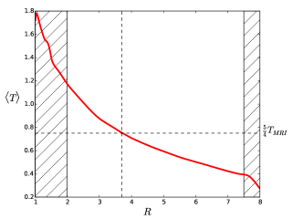
Figure 1: Temperature profile at the end of the ideal phase averaged over $200$ inner orbits. The black dashed lines show where the mean temperature is equal to $(5/4)T_{\textrm{MRI}}$. The hashed regions on both sides of the figure corresponds to the buffer zones.

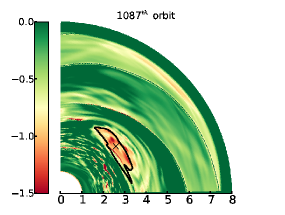
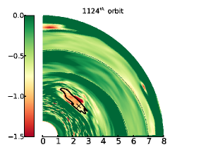
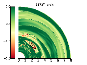
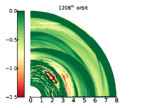
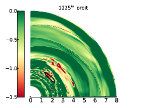
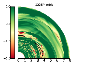
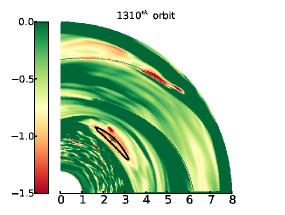
Figure 2: From left to right and top to bottom: snapshot of the relative vorticity perturbation at the $1087^{th}$, $1124^{th}$, $1173^{th}$, $1208^{th}$, $1216^{th}$, $1225^{th}$, $1228^{th}$ and $1310^{th}$ orbit. The relative vorticity perturbation has been vertically averaged. We draw with a black line the iso-contour corresponding to $80\%$ of the density maximum $\rho_{m}$. The location of the density maximum is shown by the black cross.

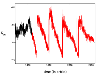
Figure 3: Radial position of the density maximum in the 3D run during the static dead-zone phase (in black) and the self-consistent phase (red curve).

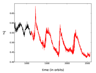
Figure 4: Temperature averaged over the vortex area in the 3D run during the static dead zone phase (in black) and the self-consistent phase (red curve).

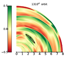
Figure 5: Snapshot of the relative density perturbation at the $1310^{th}$ orbit. The relative density perturbation has been vertically averaged. we draw with a black line the iso-contour of $80\%$ of density maximum $\rho_{m}$. The location of the density maximum is shown by the black cross.

In the final phase of the simulation we restart the simulation at $t=1100$ inner orbits and close the feedback loop: the resistivity is now a function of temperature according to Eq. (6). With this configuration, Faure et al. (2014) have shown that the dead zone inner edge moves radially before stalling at a critical radius where the gas temperature is

$$T(R_{c})=\frac{5}{4}T_{\text{MRI}}\,.$$ (9)

That critical temperature is shown on figure 1 and gives $R_{c}=3.7$. In practice, we found that the dead/active interface initially located at $R=3.5$ remains at that position over the simulation.

We found that the vortex formed during the static dead-zone step immediately begins to migrate inward. Its behavior is illustrated by the sequence of successive snapshots displayed in figure 2 where we plot the vertically integrated vertical relative vorticity $\delta\omega_{z}$ of the gas

$$\delta\omega_{z}=\frac{\mbox{\boldmath{$\nabla$}}\mbox{\boldmath{$\times$}}\mbox{\boldmath{$v$}}-\mbox{\boldmath{$\nabla$}}\mbox{\boldmath{$\times$}}\mbox{\boldmath{$v_{K}$}}}{|\mbox{\boldmath{$\nabla$}}\mbox{\boldmath{$\times$}}\mbox{\boldmath{$v_{K}$}}|}\mbox{\boldmath{$\cdot$}}\mbox{\boldmath{$e_{z}$}}\,,$$ (10)

where $v_{K}$ stands for the Keplerian velocity. The first five panels of figure 2 clearly show the vortex’s migration into the active zone. Note also that as it moves toward the star the vortex becomes smaller and smaller until it disappears after $150$ orbits (panel $6$). But by this stage a new vortex has begun to form at the dead-zone inner edge (panel $7$) and shortly begins its inward migration about ten inner orbits later (panel $8$). Following snapshots (not shown) indicate that it will also penetrate into the active zone before being similarly disrupted.

In figure 3, we plot the evolution of the vortex’s radial position $R_{\text{vort}}$ with time. This is calculated from the position of the density maximum rather than the vorticity minima because the turbulent fluctuations in the active zone can complicate the identification of the vortex. Figure 3 shows that vortices follow a cycle of formation, migration, and disruption with a period of about $200$ inner orbits. Vortices migrate inwards with a velocity $\sim 10^{-3}R_{f}\Omega_{f}$ (where $R_{f}$ and $\Omega_{f}$ respectively stands for the vortex formation radius and the angular velocity at that location) from $R\sim 3.7$ to $R\sim 2.6$, which corresponds to about $3$ scale heights at that location.

By definition, the temperature within the vortex at the formation location is below the MRI activation threshold (simply because the vortex forms in the dead zone) and the flow is relatively laminar. Heating inside the vortex is consequently low while the cooling rate is slightly increased because of its larger density compared to its surroundings. The combination of such reduced heating and increased cooling rates induces a temperature decrease within the vortex during its migration, as shown in figure 4. This causes the temperature in the vortex to remain smaller that $T_{MRI}$ during its lifetime. The typical cooling rate is of order $4.5\times 10^{-3}T_{\textrm{MRI}}\Omega_{0}$ which results in the vortex temperature decreasing by about $20\%$ by the time it disrupts. Note also the secular decrease in the vortex temperature over many cycles. This indicates that the vortices’ properties are still evolving cycle after cycle which raises the question of the existence of a stationary regime. We will come back to this issue in section 3 by performing 2D long term simulations.

Finally, we note that the temperature in the dead zone is strongly correlated with the presence of the vortex. Indeed, dead-zone temperatures increase from $T\sim 0.4$, when the vortex is weak at the end of its lifespan, to $T\sim 0.7$ just after a new one has formed. This is due to the presence of a pattern of strong density waves excited by the vortex (see the map of the density perturbations $\delta\rho/\langle\rho\rangle$ on figure 5). The density increase at the crest of these waves is significantly larger ($\sim 50\%$ of the local density) than described in Faure et al. (2014) in the absence of a vortex (only $\sim 10\%$ of the local density). These waves provide an additional source of heating and explain the warmer dead zone temperatures we obtain here.

3 The 2D simulation

In the 3D simulation, the flow is complex and the different physics — turbulence, MHD, and thermodynamics — are difficult to disentangle. In addition, the large computational cost associated with such simulations precludes long term integration. For example, the temperature evolution displays a systematic drift over a few cycles (see figure 4), thus raising the question of whether the system is able to settle into a quasi steady state, or whether the cycle described in the previous section is transient. In order to answer these questions, we present a non-magnetized laminar 2D viscous simulation which also reproduces the vortex cycles. The simpler setup eases the interpretation of the results and their long term relevance and highlights potential limitations to our simulations. In this section, we briefly present the 2D model before describing in detail the formation, migration and disruption phases of a typical cycle in that situation.

3.1 Setup and run parameters

We performed a purely hydrodynamic laminar 2D simulation of a PP disk, similar in every other way to the 3D simulations of Section 2. The evolution of the disk model described below is calculated using the uniform grid version of the RAMSES code. The equations we solve are:

$$\frac{\partial\Sigma}{\partial t}+\mbox{\boldmath{$\nabla$}}\mbox{\boldmath{$\cdot$}}(\Sigma\mbox{\boldmath{$v$}}) = 0$$ (11)

$$\frac{\partial\Sigma\mbox{\boldmath{$v$}}}{\partial t}+\mbox{\boldmath{$\nabla$}}\mbox{\boldmath{$\cdot$}}(\Sigma\mbox{\boldmath{$v$}}\mbox{\boldmath{$v$}})+\mbox{\boldmath{$\nabla$}}P = -\Sigma\mbox{\boldmath{$\nabla$}}\Phi+\mbox{\boldmath{$\nabla$}}\tau$$ (12)

$$\frac{\partial E}{\partial t}+\mbox{\boldmath{$\nabla$}}\mbox{\boldmath{$\cdot$}}\left[(E+P)\mbox{\boldmath{$v$}}\right] = -\Sigma\mbox{\boldmath{$v$}}\cdot\nabla\Phi-{\cal L}+\mbox{\boldmath{$\nabla$}}\mbox{\boldmath{$\cdot$}}(\tau\cdot\mbox{\boldmath{$v$}})$$ (13)

where $\tau$ is the Navier-Stokes stress tensor and $\Sigma$ the disk surface density. We use the viscous prescription as a crude model of both turbulent angular momentum transport and heating. The kinematic viscosity radial profile is calculated using

$$\nu=\langle\alpha\rangle_{t}c_{s}^{2}/\Omega$$ (14)

where $\langle\alpha\rangle_{t}$ is the $\alpha$ profile azimuthally, vertically and time averaged over the last $200$ orbits of the 3D static dead zone step. Here, $c_{s}$ and $\Omega$ are the local sound speed and the angular frequency. In the 3D static dead-zone step the vortex launches waves that significantly increase the angular momentum transport in the dead zone (see Faure et al., 2014). Hence the $\langle\alpha\rangle_{t}$ profile has two contributions coming from the turbulence and from the waves. In order to remove the wave contribution in the 2D simulations, which will emerge self-consistently from the vortex, we take $\langle\alpha\rangle_{t}=0$ outward of $R=3.5$. In the disk active zone, $\langle\alpha\rangle_{t}$ steadily decreases from about $0.04$ at $R\sim 2$ to $0.01$ at $R=3.5$. The viscosity jump at $R=3.5$ leads to the formation of a pressure/density bump at the outer edge of the viscous region (or, equivalently, at the inner edge of the inviscid/dead zone). We checked that the bump mass-loading rate is identical to that obtained in the 3D simulations, thus validating the $\alpha$–prescription. This corresponds to the static dead-zone phase of Section 2.

As soon as the density bump has reached five times the initial local density (which occurs at $t=1000$), we add a random velocity perturbations at the position of the bump to trigger the RWI and then close the feedback loop between resistivity and temperature by imposing:

$$\nu(T)=\begin{cases}\langle\alpha\rangle_{t}c_{s}^{2}/\Omega\,\,\,\,\textrm{if}\,\,\,T>T_{\text{MRI}}\\ 0\,\,\,\,\,\textrm{otherwise}.\end{cases}$$ (15)

The perturbation amplitude equals $10\,\%$ of the sound speed so that it mimics the velocity fluctuations induced by the turbulence on the bump. The influence of the initial bump size on the results will be discussed in section 3.3. We have hence entered the analogue of the self-consistent dead-zone phase of Section 2. A vortex forms at $R\sim 4$ in a few tens of orbits. We concentrate in the following section on a detailed analysis of this phase, for which the idealized conditions of the 2D simulations provide a favourable environment.

3.2 Vortex formation

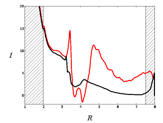
Figure 6: Radial profiles of $\mathcal{I}$ at the $1000^{th}$ orbit (red curve) and after the simulation has reached a quasi-steady state (black curve). $\mathcal{I}$ is averaged azimuthally for both cases.

Figure 7: Evolution of the logarithm of the vorticity perturbation $\delta\omega=\omega_{\textrm{max}}(R_{\text{vort}})-\omega_{\textrm{min}}(R_{\text{vort}})$ at the bump location in the 2D viscous simulation. The best fit of the linear part of the amplitude growth is plotted in black and display a slope equal to $\gamma/\Omega(R_{f})=0.2$.

The origin of the vortex forming at the dead/active interface is most likely due to the RWI (Lyra & Mac Low, 2012; Regály et al., 2012). A 2D adiabatic disk is unstable to the RWI where

$$\mathcal{I}=\frac{\Sigma\,(\nabla\times\mathbf{v})\cdot\mathbf{e_{z}}}{P^{\frac{2}{\gamma}}},$$ (16)

a conserved quantity similar to the potential vorticity, possesses a local extremum (Lovelace et al., 1999). Here $\Sigma$ is the equilibrium surface density and $\gamma$ is the adiabatic index. We show on figure 6 the profile of $\mathcal{I}$ at $t=1000$ (i.e. when random velocity fluctuations are added to the flow). Aside from small-scale variations, $\mathcal{I}$ possesses a deep and long-lasting trough at the vortex location, strong evidence that the RWI is active and generates the vortex. Note that our simulations are diabatic, and hence do not strictly conserve $\mathcal{I}$, but that this fact does not impinge on (and in fact probably aids) instability here. In the 3D simulation, the vortex and the bump form simultaneously which complicates a clear identification of the RWI’s linear phase. Nonetheless, the profile of $\mathcal{I}$ at the beginning of every cycle displays a similar trough at the position where the next vortex will form (not shown). Taken together, the results of the 2D and 3D simulations consistently point toward the RWI as being responsible for the vortex growth in our simulations.

The growth of vorticity perturbations are presented in figure 7. The perturbation grows exponentially with a growth rate of about $\gamma/\Omega(R_{f})\sim 0.2$. For the density bump properties (height and width), the empirical law of Meheut et al. (2013) gives a growth rate about twice as large, such that $\gamma_{th}/\Omega(R_{f})\sim 0.5$. Note however that this relation was obtained for globally isothermal disks with a small density perturbation such as $\delta\rho/\rho<0.3$. In our 2D simulation the density bump is $10$ times larger and the temperature gradient at the dead zone inner edge is significant. The empirical relation still provides a useful rough estimate and sanity check.

When the period of the circular motion around the vortex centre becomes comparable to the growth time scale (at $t\sim 1100$) the growth ends. The vorticity perturbation is then $\delta\omega\simeq-0.05\Omega_{0}\simeq 0.4\Omega(R_{f})$, corresponding to twice the growth rate, as noticed by Meheut et al. (2013) in their simulations. By this stage the vortex has already begun to migrate while capturing an important fraction of the initial bump’s mass:

$$\frac{\delta\rho}{\langle\rho(Rm)\rangle}=\frac{\rho_{\textrm{max}}(R_{\text{vort}})-\rho_{\textrm{min}}(R_{\text{vort}})}{\langle\rho(Rm)\rangle}\sim 0.4\,,$$ (17)

thus leaving about $60\%$ of the bump mass behind at $R=4$.

3.3 Vortex migration and disruption

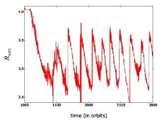
Figure 8: Radial position of the density maximum in the 2D viscous simulation using the RAMSES code.

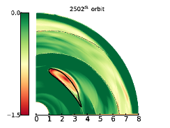
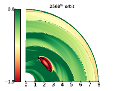
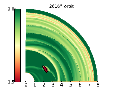
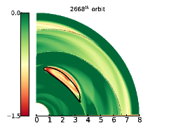
Figure 9: From left to right and top to bottom: snapshot of the relative vorticity perturbation at the $t=2502$, $2568$, $2626$ and $2668$. The relative vorticity perturbation has been vertically averaged. We draw with a black line the iso-contour of $80\%$ of density maximum $\rho_{m}$. The location of the density maximum is shown by the black cross.

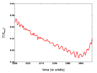
Figure 10: Evolution of the mean temperature inside the vortex during the cycle starting at the $t=2500^{th}$ inner orbit.

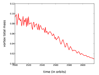
Figure 11: Evolution of the vortex total mass over the cycle starting at $t=2500$, given in unit of the initial disk mass. It is found to decrease steadily during the vortex migration.

After the first appearance of a vortex, we observe during the remainder of the 2D simulation a vortex life cycle similar to that obtained in the 3D simulation. As in the 3D simulation, the cycle properties change over the first few cycles, before the disk relaxes into a well-defined quasi-periodic state (see figure 8). During that quasi-periodic evolution, the profile of $\mathcal{I}$ at the beginning of a cycle has converged to the black curve of figure 6. The existence of a minimum of $\mathcal{I}$ at a well defined radius during the remainder of the the disk evolution shows that the conditions for vortex formation persist to late times, presumably driven by the continuing accretion mismatch at this point. The important difference is that the profile of the black curve is self–consistently obtained as a result of the disk evolution. Additional simulations starting with different bump sizes were found to exhibit different relaxation phases but all converged to the same quasi-periodic state. These results, obtained using the 2D simulation, strongly suggest that the 3D simulation of section 2 would also evolve toward a quasi stationary state if evolved for longer. Indeed, during this relaxation phase, the vortex migration range is similar to that observed in the 3D simulation. Forming at $R\sim 3.7$, vortices migrate inwards to $R\sim 2.7$. However, such a similarity does not extend to all the simulation diagnostics. For example, the cycle period is two times shorter and vortices migrate twice as fast than vortices in the 3D run. We will come back to this issue in the discussion.

We now investigate the properties of the quasi-periodic phase by focusing on one cycle, starting at $t=2500$. At that time, a vortex has formed and is about to start migrating inwards. Its relative density perturbation at this point is $\sim 0.4$. Figure 9 presents a series of snapshots showing the vorticity in the disk at four different times. The first panel illustrates the state of the disk at the beginning of the vortex: it is clear that a vortex exists at $R=3.7$. In panels 2 and 3 ($50$ and $100$ orbits later) the vortex has drifted closer to the star and has shrunk as it does so. Finally, the last panel shows the vortex has disappeared but a new vortex has formed at a larger radii at the interface. Overall, the evolution is very similar to that obtained in the 3D simulation (see figure 2). As shown in figure 10, the similarity extends to the temperature evolution of the vortex: as in the 3D simulation, the vortex cools while it moves to hotter region. The cooling rate during the stationary cycles is found to be $\approx 6\times 10^{-3}T_{\textrm{MRI}}\Omega_{0}$, i.e. slightly larger than obtained in the 3D simulations. Finally, we show in figure 11 the evolution of the mass trapped inside the vortex. As suggested by the snapshots shown on figure 9, the vortex loses mass during the cycle.

3.4 A numerical test

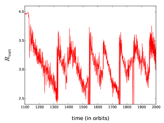
Figure 12: Radial position of the density maximum in the 2D viscous simulation using the PLUTO code.

In order to check the reliability of our simulations, we have reproduced the simulation presented in this section using the PLUTO code (Mignone et al., 2007). For this run, we used a simplified function for $\langle\alpha\rangle_{t}$:

$$\langle\alpha\rangle_{t}=\begin{cases}\alpha_{t}\left(\frac{R}{R_{0}}\right)^{-1.5}\,\,\,\,\textrm{if}\,\,\,R<R_{1}\\ \alpha_{e}\left[1-\tanh\left(\frac{R-3.2R_{0}}{1.5R_{0}}\right)\right]\left(\frac{R}{R_{0}}\right)^{-1.5}\,\textrm{if}\,\,\,R_{1}<R<R_{2}\\ 0\,\,\,\,\,\,\,\,\,\,\,\,\,\,\textrm{if}\,\,\,R>R_{2}\end{cases}$$ (18)

where $R_{1}=2.65R_{0}$, $R_{2}=3.44R_{0}$, $\alpha_{t}=7\times 10^{-2}$ and $\alpha_{e}=3.5\times 10^{-3}$ but otherwise solve the same set of equations (11), (12) and (13). Figure 12 shows the position of the vortex that forms in this simulation. The vortex cycle is clearly reproduced with a similar vortex migration timescale and amplitude as obtained with RAMSES. The quantitative differences between the PLUTO and the RAMSES simulations probably arise because of the adhoc radial profile of $\langle\alpha\rangle_{t}$ we used in PLUTO that is slightly different than used in RAMSES. The difference is, however, small and the similarity between the two simulations strengthens our main result: a vortex cycle emerges from the interplay between dynamics and thermodynamics at the dead zone inner edge.

4 Discussion

In this section we use the results of the previous two sections to illuminate the physical mechanism responsible for the vortex cycle.

4.1 Vortex destruction

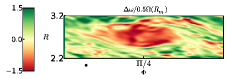
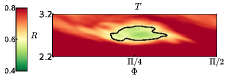
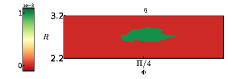
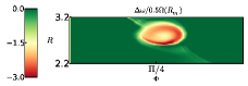
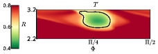
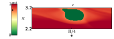
Figure 13: Top panels, from left to right: snapshots of the relative vorticity perturbation, the temperature and the resistivity in the vicinity of the vortex at the $1208^{th}$ orbit, in the 3D simulation. The fields mapped on top panels have been vertically averaged. Bottom panels, from left to right: snapshots of the relative vorticity perturbation, the temperature and the viscosity in the vicinity of the vortex at the $2597^{th}$ orbit, in the 2D simulation. We draw with a black line the iso-contour of temperature $T=T_{\textrm{MRI}}$.

First we address the issue of vortex disruption, which is a little more straightforward to understand. In both the 2D hydro and 3D MHD simulations, the vortex forms in the dead zone (modelled either as a highly resistive zone or as an inviscid region) before migrating into the active region (turbulent in the 3D case and viscous in the 2D simulation) where it gradually disrupts. Throughout its migration the interior of the vortex is either laminar or inviscid and therefore encounters turbulent interference at its outer surface. In both cases this is because the temperature in the core is below the MRI activation threshold $T_{\textrm{MRI}}$, and hence turbulence/viscosity switches off. Because of this reason vortices survive for relatively long times: in a sense, they are cool bubbles of dead zone moving inside the hot active region.

As is clear, however, from figures 2 and 8, vortices shrink in size as they migrate. Quantitative measurements using the 2D simulations showed that the vortex size changed from about $0.6H$ to about $0.25H$, at which point they dissipate. This can be understood by realizing that vortices are overwhelmed by MRI turbulence or viscous diffusion once their radius fall below a certain size. An estimate on the critical size can be obtained by equating the turbulent/viscous speed external to the vortex ($\sim\nu/s$) with the typical vortex circulation speed, estimated from simulations ($\gtrsim s\,\Omega$). We find the critical vortex size $s_{\textrm{crit}}$ is given by

$$s_{\textrm{crit}}\sim\sqrt{\langle\alpha\rangle_{t}}H\sim 0.2\,H\,.$$ (19)

This rough estimate is broadly in agreement with the results of the simulation. We hence conclude that once a vortex shrinks by about three times its original size it diffuses away in the active zone.

An estimate on the vortex lifetime is tied to the speed at which the vortex evolves, in particular to the speed at which it loses mass and shrinks. The shrinking of the vortex is possibly due to the gradual breakdown of the vortical flow via turbulent/viscous diffusion at the vortex surface. Here there appears a strong shear layer (see first panel in figure 13). Thus the vortex is destroyed gradually from the outside in. And as the outer layers disintegrate they release their mass into the surrounding active medium. A lower limit for the vortex lifetime is thus provided by the diffusion timescale of vorticity over the vortex size. Using the $\alpha$ prescription, it can be written as

$$\frac{T_{d}}{T_{orb}}=\frac{s^{2}}{\nu T_{orb}}=\frac{1}{2\pi\langle\alpha\rangle_{t}}\left(\frac{s}{H}\right)^{2}\left(\frac{R_{f}}{R_{0}}\right)^{1.5}\,.$$ (20)

For the parameters of the vortex we obtained in both the 2D and 3D simulations ($s\sim 0.5H$, $R_{f}\sim 4$), this gives an estimated destruction timescale of about $30$ orbits. Of course, this is much shorter than the typical lifetime of about $300$ orbits we obtained in the 3D simulations (see figure 3) or $150$ orbits found in the 2D simulation (see figure 11), owing to the fact that vorticity diffusion only occurs over a thin layer of size $\Delta s$ at the surface of the vortex. As a result, the viscosity over the vortex section is reduced by a factor $f\sim 2\Delta s/s$. The thickness of the layer $\Delta s$ is very difficult to estimate. As illustrated by the snapshots of figure 9, it is probably different in the 2D and 3D simulations. It might also be affected by numerical diffusion in our simulations. Nevertheless, its smallness significantly increases the vortex lifetime compared to the estimate given above, and might also account, at least partly, for the different vortex lifetimes we find in the 2D and 3D simulations.

4.2 Vortex migration

Model	Cooling function	p value	Migration rate
			(in $R_{f}\Omega_{f}$)
ST2D	Locally isothermal	-	$\sim 0$
RBD	Isentropic	$-2.75$	$-7.8\times 10^{-5}$
PLP1	Isothermal	$-4$	$-1.5\times 10^{-3}$
PLP2	Isothermal	$-1.5$	$-8\times 10^{-4}$
PLP3	Isothermal	$0$	$\sim 0$
PLPCOOL	$\cal L$ (see Eq. 21)	$0$	$\sim 0$
PLPCOOL+	$\cal L_{+}$ (see Eq. 22)	$0$	$-1.2\times 10^{-3}$
PLPCOOL-	$\cal L_{-}$ (see Eq. 22)	$0$	$+1.2\times 10^{-3}$

Table 1: Numerical experiments reproducing the setup of Richard et al. (2013) and Paardekooper et al. (2010) with various surface density profiles and thermodynamics. Simulations are 2D in polar coordinates and use a resolution $(N_{r},N_{\phi})=(768,1600)$.

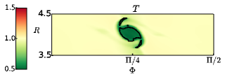
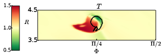
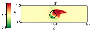
Figure 14: Snapshots of the temperature (normalized by the mean temperature) in the vortex in model PLPCOOL (top panel), PLPCOOL- (middle panel) and PLPCOOL+ (bottom panel). The black line shows an iso–vorticity contour where the vorticy is equal to the opposite of the vorticity of the background Keplerian shear profile.

We now address the question of the vortex migration process. The simple fact that we find any migration at all in our simulations is surprising by itself. Indeed, all vortices starts their journey upon a surface density maximum, which according to the isothermal simulations in Paardekooper et al. (2010) should fix the vortex in place. Generally, isothermal vortices migrate toward high pressure regions, because of asymmetric density wave launching. This result appears to be confirmed by Lyra & Mac Low (2012), who report no migration of vortices in their locally isothermal MRI-turbulent simulations of the inner dead-zone interface, and also by Meheut et al. (2012a), who considered the long-term evolution of a RWI vortex in barotropic isentropic disks. However, recently Richard et al. (2013) reported inward migration in their adiabatic runs of RWI vortex formation. Here, however, the vortex, by absorbing all the bump material, destroys the adverse pressure gradient that would prevent its migration. In our runs, the vortical perturbation is similar but the bump size at the beginning of a cycle is significantly bigger and the vortices start their migration before they completely absorb the bump mass. As sanity checks, we have successfully reproduced the results of Richard et al. (2013) albeit in a 2D simulation (see model RBD in table 1). Finally, the migration rate we measure is about $10$ times higher than in Richard et al. (2013). Questions therefore remain: why are vortices migrating in our simulations, and why do they migrate so fast?

We focus on the 2D simulations, as the vertical dimension and MHD turbulence are likely to complicate the picture. Several additional numerical experiments were performed, detailed in table 1. First, at $t=1000$ in our standard 2D run (see section 3.1), we have frozen the temperature and calculated the subsequent evolution of the vortex using a locally isothermal equation of state (model STD2D). We found the vortex remained at its formation location. Immediately, it is clear that the gas thermodynamics is crucial to the migration process.

To further test that idea, we performed a set of simulations that reproduce the setup described by Paardekooper et al. (2010). Within an isothermal and inviscid 2D disk, we initialized a strong vortex by introducing a vortical velocity perturbation. For three different exponents of the background density radial profile (models PLP1, PLP2 and PLP3), we measured three vortex migration velocities that are in agreement with the results reported by Paardekooper et al. (2010). In particular, the zero pressure-gradient case (model PLP3) is almost neutral in the sense that the migration rate of the vortex is vanishingly small.

Next, in order to interrogate the role of the thermodynamics, we relaxed the assumption of isothermality and modified the cooling function ${\cal L}$ in Eq. (13) so that it takes the form

$$\cal L=\begin{cases}(T-T_{b}/2)/\tau_{v}\,\,\,\,\textrm{if}\,\,\,\mbox{\boldmath{$\delta\omega$}}.\mbox{\boldmath{$e_{z}$}}<-1\\ (T-T_{b})/\tau_{d}\,\,\,\,\,\,\,\,\,\textrm{otherwise}.\end{cases}$$ (21)

$T_{b}$ is the gas background temperature, averaged azimuthally. This is model PLPCOOL, and its piece-wise cooling law, by depending on the strength of vorticity, forces the vortex to possess a different temperature than its surrounding. If we take $\tau_{v}=10$ orbits and $\tau_{d}=1$ orbit, the vortex is cooler than its surroundings which should relax to the initial temperature profile (see top panel in figure 14). In this case, the vortex stays at its initial position, showing that a change of the bulk temperature of the vortex is not enough by itself to affect its migration. We then introduce an azimuthal asymmetry in the vortex cooling by further modifying the cooling function:

$$\cal L_{\pm}=\begin{cases}(T-T_{b}(1\pm\frac{\mbox{\boldmath{$v$}}\cdot\mbox{\boldmath{$e_{R}$}}}{2|\mbox{\boldmath{$v$}}\cdot\mbox{\boldmath{$e_{R}$}}|}))/\tau_{v}\,\,\,\,\textrm{if}\,\,\,\mbox{\boldmath{$\delta\omega$}}.\mbox{\boldmath{$e_{z}$}}<-1\\ (T-T_{b})/\tau_{d}\,\,\,\,\,\,\,\,\,\textrm{otherwise}.\end{cases}$$ (22)

The resulting relative temperature perturbations differ widely as illustrated on the middle and bottom panels of figure 14. With this new cooling prescription, we found significant inward or outward migration of the vortex depending on the sign in Eq.(22), despite the vanishing radial pressure gradient. If the vortex is hotter in the region downstream of its core (in the sense of the background rotation) than the surrounding gas while being cooler in the upstream region (case PLPCOOL+), the vortex migrates inward. In the opposite situation (case PLPCOOL-), the vortex migrates outward with the same velocity. The migration speed is significant and in fact comparable in magnitude (to less than a factor of two) to the isothermal case when $p=-1.5$ (see table 1).

We conclude from this series of experiments that diabaticity can play an important role in vortex migration. In particular, an azimuthal temperature gradient may help the vortex to overcome pressure gradients that would otherwise hold it in place. The detailed and quantitative understanding of these effects is largely beyond the scope of this paper and requires additional more specialised simulations. However, it seems likely that a migration mechanism is at work in our simulations that differs from that discussed in earlier work. It is likely that the new effect is associated with the baroclinic term in the vorticity equation, which vanishes in the barotropic flow of model PLP3 but is nonzero in model $\textrm{PLPCOOL}\pm$. This constitutes the only difference between the two experiments. We speculate that the cooler temperatures in our vortex solutions and the sharp temperature gradient at its surface would mean that the vortex circulation is modified, with fluid parcels having to turn abruptly. This could modify the position of the sonic lines and, along with the modified vortex shape (see the black lines on figure 14), maybe strengthen their asymmetry and trigger radial migration.

In addition, the importance of thermodynamics effects is consistent with the differences we find between the 2D and 3D simulations, particularly when it comes to comparing the migration velocities of the vortex. Obviously, the thermal history of the vortices in these simulations differ on account of the two distinct heating processes (turbulent and ohmic dissipation in the 3D case, viscous dissipation in the 2D simulation). The fact that the different baroclinic terms might result in different vortensity evolution is partly supported by the left panels of figure 13 that shows the different vorticity field distribution within a single vortex in the two cases.

4.3 The case of the static dead zone phase

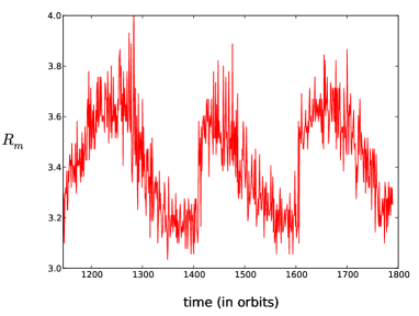
Figure 15: Radial position of the density maximum in the 3D run during the static dead zone step.

We finally end the discussion by noting that our findings naturally explain the difference between the static dead zone step and the self-consistent step. Indeed, a vortex is observed to grow in the former. The question is: why does not this vortex migrate into the dead zone? We have checked this issue and we have found that, in fact, vortices do migrate inward in this case as well. This is illustrated by figure 15. The difference in this case is that the vortex migration range is much smaller than in the 3D case: the vortex disappears upon reaching $R\sim 3.1$ (as opposed to $\sim 2.7$ in the 3D case). This is because the resistivity is not a function of temperature in this case, but a function of position only: as the vortex penetrates into the active zone, its resistivity drops to zero with renders the flow vulnerable to MRI induced velocity fluctuations. As a result, vortices formed during the static dead zone step have a smaller lifetime (of order $100$ orbits, as opposed to the $300$ orbits measured during the self-consistent step) when they enter the active zone.

5 Conclusion

In this paper, we have performed a non-ideal MHD simulation of the region centred around the dead-zone inner edge of a protoplanetary disk. In accordance with previously published work (Lyra & Mac Low, 2012), we find that a vortex forms at the dead zone inner edge. Our simulation reveals that the vortex is not affixed to the pressure maximum as one would expect from the results of Paardekooper et al. (2010) but migrates inward. It penetrates into the active zone where it is gradually destroyed by turbulent motions. A few orbits later a new vortex forms at the interface and follows the same evolution, thereby creating what we have called a “vortex cycle”: formation, migration, and disruption follow each other and comprise a quasi-periodic disk evolution.

We find that the vortex cycle does not exist in isothermal simulations of the dead zone inner edge. This is because the vortex stays at its formation location without migrating inward. In fact, we have been unable to design any test in which a vortex moves in a uniform pressure background when its temperature is equal to that of its surroundings. Vortex migration seems to occur only if the vortex temperature is different from (and maybe even free to evolve independantly of) the temperature of its environment. A systematic study and a detailed understanding of vortex migration rates in such specific environments is needed. Indeed, we caution the reader that simulations using a different cooling function may exhibit cycles with very different properties. Moreover, we completely neglected heat diffusion in the present paper, and particularly radiative diffusion. Even if vortices forming in a optically thick region such as the dead zone inner edge are likely to be cooler than the turbulent region in which they will penetrate, radiative diffusion will act as a heating source that will help decrease the difference between the vortex temperature and the temperature of its surroundings. If the heat diffusion timescale is shorter than the vortex cycle, the ionization threshold will be crossed at some point. This will quickly activate the magneto-elliptic instability (Lebovitz & Zweibel, 2004; Mizerski & Lyra, 2012), the growth rate of which (about one local orbit) is much faster than the vortex cycle timescale, and will disrupt the vortex. An accurate measurement of the cycle period and the vortex migration rate should be done using simulations including radiative transfer that properly account for the vortex thermodynamics.

An additional limitation of our work comes from geometry itself. The 3D simulation uses the cylindrical approximation. Taking into account the disk vertical structure (Richard et al., 2013; Meheut et al., 2012a; Lesur & Papaloizou, 2009) will affect both the vortex properties and the shape of the dead/active interface. Along the same lines, the magnetic configuration is also known to influence the development of vortices (Lyra & Klahr, 2011; Yu & Li, 2009; Yu & Lai, 2013). For example, the presence of a net vertical flux in the inner parts might change the results presented here in surprising ways.

Before closing this paper, we speculate on the possible consequences of the vortex cycle for the dynamics of dust particles in the disk. As we already discussed, vortices such as those we see in our simulations are known to concentrate dust grains and help planet formation processes. However, we have shown here that vortices do not stay at their formation location but migrate inward, most likely carrying the dust particles they captured at the density bump. If the particles are still small once they are released by the disrupted vortex, they might continue to migrate inward due to the gas friction. The vortex cycle would then help the dust to pass across the pressure bump barrier. From this discussion, a number of questions arise:

1. What dust concentration can the vortex achieve?

The 3D bi-fluid simulations of Meheut et al. (2012b) have shown that the dust-to-gas ratio may change from $0.01$ to $1$ inside a vortex in three local orbits. This is much shorter than the cycle period, suggesting that vortices formed at the dead zone inner edge would trap the entire content of dust initially present in the bump.

1. Can dust grains embedded in the vortex become large enough as a result of collisions alone that friction becomes negligible at the time of vortex disruption?

According to 1+1D models of dust growth (e.g. Brauer et al. 2008a), the dust growth rate in laminar regions is mainly due to differential settling. Such a growth timescale can be taken as a proxy for the typical time required to grow centimetre size particles into metre size bodies within the vortex. It amounts to about a thousand years which is much longer than the cycle period of a few hundred years. This seems to suggest that particles transported by a vortex across the bump barrier would not grow significantly over one cycle. Particles would then quickly drift toward the central star and take no part in the process of planetesimal formation. A fast mechanism is needed to prevent a loss of the disk solid content. Given the large dust–to–gas ratio that are likely to be found inside vortices, such fast processes could be the streaming instability (Youdin & Johansen, 2007; Johansen & Youdin, 2007), gravitational collapse (Lyra et al., 2008) or a combination of both phenomena (Johansen et al., 2007). However, we caution the reader that gas choatic motions in the vortex resulting from sound waves may disrupt embryos formed by those mechanisms. A detailed study of the outcome of these instabilities is needed.

For such a nonlinear and complex problem, it is difficult to go beyond these simple qualitative statements. Clearly, self-consistent simulations including the vortex cycle phenomenon along with dust dynamics (including dust growth) are needed if we want to make any quantitative statement regarding the fate of dust particles at the dead-zone’s inner edge. As we already argued, such simulations will also have to properly include radiative effects since the vortex migration is sensitive to the gas thermodynamics. Such multi–fluid radiative MHD simulations are, of course, very resource demanding with present day computing resources.

References

- Balbus & Hawley (1991) Balbus, S. A. & Hawley, J. F. 1991, ApJ, 376, 214
- Balbus & Hawley (1998) Balbus, S. A. & Hawley, J. F. 1998, Reviews of Modern Physics, 70, 1
- Barge & Sommeria (1995) Barge, P. & Sommeria, J. 1995, A&A, 295, L1
- Benz (2000) Benz, W. 2000, Space Sci. Rev., 92, 279
- Brauer et al. (2007) Brauer, F., Dullemond, C. P., Johansen, A., et al. 2007, A&A, 469, 1169
- Brauer et al. (2008) Brauer, F., Henning, T., & Dullemond, C. P. 2008, A&A, 487, L1
- Brown et al. (2009) Brown, J. M., Blake, G. A., Qi, C., et al. 2009, ApJ, 704, 496
- Casassus et al. (2012) Casassus, S., Perez M., S., Jordán, A., et al. 2012, ApJ, 754, L31
- Chiang & Youdin (2010) Chiang, E. & Youdin, A. N. 2010, Annual Review of Earth and Planetary Sciences, 38, 493
- Chokshi et al. (1993) Chokshi, A., Tielens, A. G. G. M., & Hollenbach, D. 1993, ApJ, 407, 806
- de Val-Borro et al. (2007) de Val-Borro, M., Artymowicz, P., D’Angelo, G., & Peplinski, A. 2007, A&A, 471, 1043
- Dominik & Tielens (1997) Dominik, C. & Tielens, A. G. G. M. 1997, ApJ, 480, 647
- Dzyurkevich et al. (2010) Dzyurkevich, N., Flock, M., Turner, N. J., Klahr, H., & Henning, T. 2010, A&A, 515, A70
- Faure et al. (2014) Faure, J., Fromang, S., & Latter, H. 2014, A&A, 564, A22
- Fromang et al. (2006) Fromang, S., Hennebelle, P., & Teyssier, R. 2006, A&A, 457, 371
- Gammie (1996) Gammie, C. F. 1996, ApJ, 457, 355
- Garaud et al. (2013) Garaud, P., Meru, F., Galvagni, M., & Olczak, C. 2013, ApJ, 764, 146
- Goldreich & Ward (1973) Goldreich, P. & Ward, W. R. 1973, ApJ, 183, 1051
- Hayashi et al. (1985) Hayashi, C., Nakazawa, K., & Nakagawa, Y. 1985, in Protostars and Planets II, ed. D. C. Black & M. S. Matthews, 1100–1153
- Hughes & Armitage (2012) Hughes, A. L. H. & Armitage, P. J. 2012, MNRAS, 423, 389
- Inaba & Barge (2006) Inaba, S. & Barge, P. 2006, ApJ, 649, 415
- Isella et al. (2013) Isella, A., Pérez, L. M., Carpenter, J. M., et al. 2013, ApJ, 775, 30
- Johansen et al. (2004) Johansen, A., Andersen, A. C., & Brandenburg, A. 2004, A&A, 417, 361
- Johansen et al. (2007) Johansen, A., Oishi, J. S., Mac Low, M.-M., et al. 2007, Nature, 448, 1022
- Johansen & Youdin (2007) Johansen, A. & Youdin, A. 2007, ApJ, 662, 627
- Klahr & Bodenheimer (2006) Klahr, H. & Bodenheimer, P. 2006, ApJ, 639, 432
- Kornet et al. (2001) Kornet, K., Stepinski, T. F., & Różyczka, M. 2001, A&A, 378, 180
- Kothe et al. (2010) Kothe, S., Güttler, C., & Blum, J. 2010, ApJ, 725, 1242
- Kretke & Lin (2007) Kretke, K. A. & Lin, D. N. C. 2007, ApJ, 664, L55
- Kretke et al. (2009) Kretke, K. A., Lin, D. N. C., Garaud, P., & Turner, N. J. 2009, ApJ, 690, 407
- Latter & Balbus (2012) Latter, H. N. & Balbus, S. 2012, MNRAS, 424, 1977
- Lebovitz & Zweibel (2004) Lebovitz, N. R. & Zweibel, E. 2004, ApJ, 609, 301
- Lesur & Papaloizou (2009) Lesur, G. & Papaloizou, J. C. B. 2009, A&A, 498, 1
- Li et al. (2000) Li, H., Finn, J. M., Lovelace, R. V. E., & Colgate, S. A. 2000, ApJ, 533, 1023
- Lin (2012) Lin, M.-K. 2012, ApJ, 754, 21
- Lin & Papaloizou (2011) Lin, M.-K. & Papaloizou, J. C. B. 2011, MNRAS, 415, 1426
- Lovelace et al. (1999) Lovelace, R. V. E., Li, H., Colgate, S. A., & Nelson, A. F. 1999, ApJ, 513, 805
- Lyra et al. (2008) Lyra, W., Johansen, A., Klahr, H., & Piskunov, N. 2008, A&A, 491, L41
- Lyra & Klahr (2011) Lyra, W. & Klahr, H. 2011, A&A, 527, A138
- Lyra & Mac Low (2012) Lyra, W. & Mac Low, M.-M. 2012, ApJ, 756, 62
- Meheut et al. (2010) Meheut, H., Casse, F., Varniere, P., & Tagger, M. 2010, A&A, 516, A31
- Meheut et al. (2012a) Meheut, H., Keppens, R., Casse, F., & Benz, W. 2012a, A&A, 542, A9
- Meheut et al. (2013) Meheut, H., Lovelace, R. V. E., & Lai, D. 2013, MNRAS, 430, 1988
- Meheut et al. (2012b) Meheut, H., Meliani, Z., Varniere, P., & Benz, W. 2012b, A&A, 545, A134
- Mignone et al. (2007) Mignone, A., Bodo, G., Massaglia, S., et al. 2007, ApJS, 170, 228
- Mizerski & Lyra (2012) Mizerski, K. A. & Lyra, W. 2012, Journal of Fluid Mechanics, 698, 358
- Nakagawa et al. (1981) Nakagawa, Y., Nakazawa, K., & Hayashi, C. 1981, Icarus, 45, 517
- Paardekooper et al. (2010) Paardekooper, S.-J., Lesur, G., & Papaloizou, J. C. B. 2010, ApJ, 725, 146
- Pérez et al. (2014) Pérez, L. M., Isella, A., Carpenter, J. M., & Chandler, C. J. 2014, ApJ, 783, L13
- Poppe et al. (2000) Poppe, T., Blum, J., & Henning, T. 2000, ApJ, 533, 472
- Regály et al. (2012) Regály, Z., Juhász, A., Sándor, Z., & Dullemond, C. P. 2012, MNRAS, 419, 1701
- Richard et al. (2013) Richard, S., Barge, P., & Le Dizès, S. 2013, A&A, 559, A30
- Seizinger & Kley (2013) Seizinger, A. & Kley, W. 2013, A&A, 551, A65
- Sekiya (1998) Sekiya, M. 1998, Icarus, 133, 298
- Stepinski & Valageas (1997) Stepinski, T. F. & Valageas, P. 1997, A&A, 319, 1007
- Takeuchi & Lin (2002) Takeuchi, T. & Lin, D. N. C. 2002, ApJ, 581, 1344
- Tanga et al. (1996) Tanga, P., Babiano, A., Dubrulle, B., & Provenzale, A. 1996, Icarus, 121, 158
- Teyssier (2002) Teyssier, R. 2002, A&A, 385, 337
- Turner et al. (2010) Turner, N. J., Carballido, A., & Sano, T. 2010, ApJ, 708, 188
- van der Marel et al. (2013) van der Marel, N., van Dishoeck, E. F., Bruderer, S., et al. 2013, Science, 340, 1199
- Varnière & Tagger (2006) Varnière, P. & Tagger, M. 2006, A&A, 446, L13
- Weidenschilling (1977) Weidenschilling, S. J. 1977, MNRAS, 180, 57
- Weidenschilling (1980) Weidenschilling, S. J. 1980, Icarus, 44, 172
- Weidenschilling & Cuzzi (1993) Weidenschilling, S. J. & Cuzzi, J. N. 1993, in Protostars and Planets III, ed. E. H. Levy & J. I. Lunine, 1031–1060
- Windmark et al. (2012) Windmark, F., Birnstiel, T., Ormel, C. W., & Dullemond, C. P. 2012, A&A, 544, L16
- Wurm et al. (2005) Wurm, G., Paraskov, G., & Krauss, O. 2005, Icarus, 178, 253
- Youdin & Johansen (2007) Youdin, A. & Johansen, A. 2007, ApJ, 662, 613
- Yu & Lai (2013) Yu, C. & Lai, D. 2013, MNRAS, 429, 2748
- Yu & Li (2009) Yu, C. & Li, H. 2009, ApJ, 702, 75
- Zsom et al. (2010) Zsom, A., Ormel, C. W., Güttler, C., Blum, J., & Dullemond, C. P. 2010, A&A, 513, A57