Foliated eight-manifolds for M-theory compactification

Abstract

We characterize compact eight-manifolds $M$ which arise as internal spaces in ${\cal N}=1$ flux compactifications of M-theory down to $\mathrm{AdS}_{3}$ using the theory of foliations, for the case when the internal part $\xi$ of the supersymmetry generator is everywhere non-chiral. We prove that specifying such a supersymmetric background is equivalent with giving a codimension one foliation $\mathcal{F}$ of $M$ which carries a leafwise $G_{2}$ structure, such that the O’Neill-Gray tensors, non-adapted part of the normal connection and the torsion classes of the $G_{2}$ structure are given in terms of the supergravity four-form field strength by explicit formulas which we derive. We discuss the topology of such foliations, showing that the $C^{\ast}$ algebra $C(M/\mathcal{F})$ is a noncommutative torus of dimension given by the irrationality rank of a certain cohomology class constructed from $\mathbf{G}$, which must satisfy the Latour obstruction. We also give a criterion in terms of this class for when such foliations are fibrations over the circle. When the criterion is not satisfied, each leaf of $\mathcal{F}$ is dense in $M$.

Introduction

$\mathcal{N}=1$ compactifications of $M$-theory on eight-manifolds Becker1 ; Becker2 ; Constantin ; MartelliSparks ; Tsimpis hold particular interest due to their potential relation to F-theory Bonetti and since they provide nontrivial testing grounds for many physical and mathematical ideas. In this paper, we reconsider the class of supersymmetric compactifications of eleven-dimensional supergravity down to $\mathrm{AdS}_{3}$ spaces — which was pioneered in MartelliSparks — using the theory of foliations. Our purpose is to give a complete mathematical characterization of those oriented, compact and connected eight-manifolds $M$ which satisfy the corresponding supersymmetry conditions, in the case when the internal part of the supersymmetry generator is everywhere non-chiral — thus providing a supersymmetric realization of some of the ideas proposed in Grana .

Using a combination of techniques from the theory of Kähler-Atiyah algebras and of $G$-structures, an everywhere non-chiral Majorana spinor $\xi$ on $M$ can be parameterized by a one-form $V$ whose kernel distribution $\mathcal{D}$ carries a $G_{2}$ structure. We show that the condition that $\xi$ satisfies the supersymmetry equations is equivalent with the requirement that $\mathcal{D}$ is Frobenius integrable (namely, a certain one-form proportional to $V$ must belong to a cohomology class specified by the supergravity four-form field strength $\mathbf{G}$) and that the O’Neill-Gray tensors of the codimension one foliation $\mathcal{F}$ which integrates $\mathcal{D}$, the non-adapted part of the normal connection of $\mathcal{F}$ as well as the torsion classes of the $G_{2}$ structure of $\mathcal{D}$, be given in terms of $\mathbf{G}$ through explicit expressions which we derive. In particular, we find that the leafwise $G_{2}$ structure is “integrable”, in the sense $\boldsymbol{\tau}_{2}=0$, i.e. that it belongs to the Fernandez-Gray class $W_{1}\oplus W_{3}\oplus W_{4}$ (in the notation of FG ) — a class of $G_{2}$ structures which was studied in detail in FriedrichIvanov1 ; FriedrichIvanov2 . More precisely, we find that this leafwise $G_{2}$ structure is conformally co-calibrated, thus being — up to a conformal transformation — of the type studied in GrigorianCoflow . Furthermore, the field strength $\mathbf{G}$ can be determined in terms of the geometry of the foliation $\mathcal{F}$ and of the torsion classes of its longitudinal $G_{2}$ structure, provided that $\mathcal{F}$ and this $G_{2}$ structure satisfy some purely geometric conditions, the form of which we derive explicitly. These results complete the analysis initiated by MartelliSparks , giving a full solution to the problem via three theorems which we prove rigorously.

We point out that existence of a nowhere-chiral Majorana spinor on $M$ is obstructed by a certain class having its origin in Novikov theory. We also discuss the topology of $\mathcal{F}$, giving a criterion in terms of $\mathbf{G}$ which allows one to decide when the leaves of $\mathcal{F}$ are compact or dense in $M$ and thus when it is possible to present $\mathcal{F}$ as a fibration over the circle. When $\mathcal{F}$ has dense leaves, its leaf space admits a non-commutative geometric description in terms of a $C^{\ast}$ algebra $C(M/\mathcal{F})$ which is Morita equivalent with that of a non-commutative torus whose dimension is determined by the four-form $\mathbf{G}$.

The paper is organized as follows. Section 1 gives a brief review of the class of compactifications we consider. Section 2 discusses a geometric characterization of spin 1/2 Majorana spinors on $M$ which are nowhere-chiral and everywhere of norm one. It also gives the description of such spinors through the Kähler-Atiyah algebra of $M$ and a certain parameterization which is essential for the rest of the paper. Section 3 gives our equivalent characterizations of the supersymmetry conditions, thus providing a complete geometric description of such supersymmetric backgrounds; it also describes the Latour obstruction to the existence of solutions. Section 4 discusses the topology of the foliation $\mathcal{F}$, giving a flux criterion for compactness of the leaves and the non-commutative geometric model of its leaf space. Section 5 provides a brief comparison with previous work, while Section 6 concludes. The appendices contain various technical details.

Notations and conventions.

Throughout this paper, $M$ denotes an oriented, connected and compact smooth manifold (which will mostly be of dimension eight), whose unital commutative $\mathbb{R}$-algebra of smooth real-valued functions we denote by ${{\cal\mathcal{C}}^{\infty}(M,\mathbb{R})}$. All vector bundles we consider are smooth. We use freely the results and notations of ga1 ; ga2 ; gf , with the same conventions as there. To simplify notation, we write the geometric product $\diamond$ of loc. cit. simply as juxtaposition while indicating the wedge product of differential forms through $\wedge$. If $\mathcal{D}\subset TM$ is a Frobenius distribution on $M$, we let $\Omega(\mathcal{D})=\Gamma(M,\wedge\mathcal{D}^{\ast})$ denote the ${{\cal\mathcal{C}}^{\infty}(M,\mathbb{R})}$-module of longitudinal differential forms along $\mathcal{D}$. When $\dim M=8$, then for any 4-form $\omega\in\Omega^{4}(M)$, we let $\omega^{\pm}\stackrel{{\scriptstyle{\rm def.}}}{{=}}\frac{1}{2}(\omega\pm\ast\omega)$ denote the self-dual and anti-selfdual parts of $\omega$ (namely, $\ast\omega^{\pm}=\pm\omega^{\pm}$). This paper assumes some familiarity with the theory of foliations, for which we refer the reader to CC1 ; CC2 ; Tondeur ; Moerdijk ; Bejancu .

1 Basics

We start with a brief review of the set-up, in order to fix notation. As in MartelliSparks ; Tsimpis , we consider 11-dimensional supergravity sugra11 on an eleven-dimensional connected and paracompact spin manifold $\mathbf{M}$ with Lorentzian metric $\mathbf{g}$ (of ‘mostly plus’ signature). Besides the metric, the classical action of the theory contains the three-form potential with four-form field strength $\mathbf{G}\in\Omega^{4}(\mathbf{M})$ and the gravitino $\mathbf{\Psi}$, which is a Majorana spinor of spin $3/2$. The bosonic part of the action takes the form:

$$S_{\rm bos}[\mathbf{g},\mathbf{C}]=\frac{1}{2\mathbf{\kappa}_{11}^{2}}\int_{\mathbf{M}}R\boldsymbol{\nu}-\frac{1}{4\mathbf{\kappa}_{11}^{2}}\int_{\mathbf{M}}\big{(}\mathbf{G}\wedge\star\mathbf{G}+\frac{1}{3}\mathbf{C}\wedge\mathbf{G}\wedge\mathbf{G}\big{)}~{}~{},$$

where $\mathbf{\kappa}_{11}$ is the gravitational coupling constant in eleven dimensions, $\boldsymbol{\nu}$ and $R$ are the volume form and the scalar curvature of $\mathbf{g}$ and $\mathbf{G}=\mathrm{d}\mathbf{C}$. For supersymmetric bosonic classical backgrounds, both the gravitino and its supersymmetry variation must vanish, which requires that there exist at least one solution $\boldsymbol{\eta}$ to the equation:

$$\delta_{\boldsymbol{\eta}}\mathbf{\Psi}\stackrel{{\scriptstyle{\rm def.}}}{{=}}\mathfrak{D}\boldsymbol{\eta}=0~{}~{},$$ (1)

where $\mathfrak{D}$ denotes the supercovariant connection. The eleven-dimensional supersymmetry generator $\boldsymbol{\eta}$ is a Majorana spinor (real pinor) of spin $1/2$ on $\mathbf{M}$.

As in MartelliSparks ; Tsimpis , consider compactification down to an $\mathrm{AdS}_{3}$ space of cosmological constant $\Lambda=-8\kappa^{2}$, where $\kappa$ is a positive real parameter — this includes the Minkowski case as the limit $\kappa\rightarrow 0$. Thus $\mathbf{M}=N\times M$, where $N$ is an oriented 3-manifold diffeomorphic with $\mathbb{R}^{3}$ and carrying the $\mathrm{AdS}_{3}$ metric $g_{3}$ while $M$ is an oriented, compact and connected Riemannian eight-manifold whose metric we denote by $g$. The metric on $\mathbf{M}$ is a warped product:

$$\mathrm{d}\mathbf{s}^{2} = e^{2\Delta}\mathrm{d}s^{2}~{}~{}~{}{\rm where}~{}~{}~{}\mathrm{d}s^{2}=\mathrm{d}s^{2}_{3}+g_{mn}\mathrm{d}x^{m}\mathrm{d}x^{n}~{}~{}.$$ (2)

The warp factor $\Delta$ is a smooth real-valued function defined on $M$ while $\mathrm{d}s_{3}^{2}$ is the squared length element of the $\mathrm{AdS}_{3}$ metric $g_{3}$. For the field strength $\mathbf{G}$, we use the ansatz:

$$\mathbf{G}=\nu_{3}\wedge\mathbf{f}+\mathbf{F}~{}~{},~{}~{}~{}~{}\mathrm{with}~{}~{}\mathbf{F}\stackrel{{\scriptstyle{\rm def.}}}{{=}}e^{3\Delta}F~{}~{},~{}~{}\mathbf{f}\stackrel{{\scriptstyle{\rm def.}}}{{=}}e^{3\Delta}f~{}~{},$$ (3)

where $f\in\Omega^{1}(M)$, $F\in\Omega^{4}(M)$ and $\nu_{3}$ is the volume form of $(N,g_{3})$. For $\boldsymbol{\eta}$, we use the ansatz:

$$\boldsymbol{\eta}=e^{\frac{\Delta}{2}}(\zeta\otimes\xi)~{}~{},$$

where $\xi$ is a Majorana spinor of spin $1/2$ on the internal space $(M,g)$ (a section of the rank 16 real vector bundle $S$ of indefinite chirality real pinors) and $\zeta$ is a Majorana spinor on $(N,g_{3})$.

Assuming that $\zeta$ is a Killing spinor on the $\mathrm{AdS}_{3}$ space $(N,g_{3})$, the supersymmetry condition (1) is equivalent with the following system for $\xi$:

$$\boxed{\mathbb{D}\xi=0~{}~{},~{}~{}Q\xi=0}~{}~{},$$ (4)

where

$$\mathbb{D}_{X}=\nabla_{X}^{S}+\frac{1}{4}\gamma(X\lrcorner F)+\frac{1}{4}\gamma((X_{\sharp}\wedge f)\nu)+\kappa\gamma(X\lrcorner\nu)~{}~{},~{}~{}X\in\Gamma(M,TM)$$

is a linear connection on $S$ (here $\nabla^{S}$ is the connection induced on $S$ by the Levi-Civita connection of $(M,g)$, while $\nu$ is the volume form of $(M,g)$) and

$$Q=\frac{1}{2}\gamma(\mathrm{d}\Delta)-\frac{1}{6}\gamma(\iota_{f}\nu)-\frac{1}{12}\gamma(F)-\kappa\gamma(\nu)$$

is a globally-defined endomorphism of $S$. As in MartelliSparks ; Tsimpis , we do not require that $\xi$ has definite chirality.

The set of solutions of (4) is a finite-dimensional $\mathbb{R}$-linear subspace $\mathrm{\cal K}(\mathbb{D},{Q})$ of the infinite-dimensional vector space $\Gamma(M,S)$ of smooth sections of $S$. Up to rescalings by smooth nowhere-vanishing real-valued functions defined on $M$, the vector bundle $S$ has two admissible pairings $\Scr B_{\pm}$ (see gf ; AC1 ; AC2 ), both of which are symmetric but which are distinguished by their types $\epsilon_{\Scr B_{\pm}}=\pm 1$. Without loss of generality, we choose to work with $\Scr B\stackrel{{\scriptstyle{\rm def.}}}{{=}}\Scr B_{+}$. We can in fact take $\Scr B$ to be a scalar product on $S$ and denote the corresponding norm by $||~{}||$ (see ga1 ; ga2 for details). Requiring that the background preserves exactly $\mathcal{N}=1$ supersymmetry amounts to asking that $\dim\mathrm{\cal K}(\mathbb{D},Q)=1$. It is not hard to check ga1 that $\Scr B$ is $\mathbb{D}$-flat:

$$\mathrm{d}\Scr B(\xi^{\prime},\xi^{\prime\prime})=\Scr B(\mathbb{D}\xi^{\prime},\xi^{\prime\prime})+\Scr B(\xi^{\prime},\mathbb{D}\xi^{\prime\prime})~{}~{},~{}~{}\forall\xi^{\prime},\xi^{\prime\prime}\in\Gamma(M,S)~{}~{}.$$ (5)

Hence any solution of (4) which has unit $\Scr B$-norm at a point will have unit $\Scr B$-norm at every point of $M$ and we can take the internal part $\xi$ of the supersymmetry generator to be everywhere of norm one.

Besides the supersymmetry equations (4), one has the Bianchi identity $\mathrm{d}\mathbf{G}=0$, which gives:

$$\mathrm{d}\mathbf{F}=\mathrm{d}\mathbf{f}=0~{}~{}$$ (6)

and one must impose the equations of motion:

$$\mathbf{\mathrm{d}}\star\mathbf{G}+\frac{1}{2}\mathbf{G}\wedge\mathbf{G}=0~{}~{}$$ (7)

for the supergravity three-form potential, where $\star$ is the Hodge operator of $(\mathbf{M},\mathbf{g})$. It is not hard to check that these amount to the following conditions, where $\ast$ is the Hodge operator of $(M,g)$:

$$e^{-6\Delta}\mathrm{d}(e^{6\Delta}\ast f)-\frac{1}{2}F\wedge F~{}~{}=0$$

$$e^{-6\Delta}\mathrm{d}(e^{6\Delta}\ast F)-f\wedge F~{}~{}~{}~{}=0~{}~{}.$$ (8)

Together with the supersymmetry conditions, it follows from the arguments of Eins that (1) imply the Einstein equations. It was noticed in MartelliSparks that integrating the scalar part of the Einstein equations:

$$e^{-9\Delta}\Box e^{9\Delta}+72\kappa^{2}=\frac{3}{2}||F||^{2}+3||f||^{2}$$

implies, when $\kappa=0$, that $F$ and $f$ must vanish identically on $M$ (and thus $\mathbf{G}$ must vanish identically on $\mathbf{M}$) while $\Delta$ must be constant on $M$. In that case $Q=0$ and $\mathbb{D}=\nabla^{S}$ so (4) reduce to the condition that $\xi$ is covariantly constant on $M$, which implies that each of the chiral components $\xi^{\pm}\stackrel{{\scriptstyle{\rm def.}}}{{=}}\frac{1}{2}(1\pm\gamma(\nu))\xi$ must be covariantly constant (and thus of constant norm). When $\xi$ is chiral (i.e. when $\xi^{+}=0$ or $\xi^{-}=0$), this means that $(M,g)$ has holonomy contained in $\mathrm{Spin}(7)$ (equaling $\mathrm{Spin}(7)$ iff. $M$ is simply connected), while when $\xi$ is nowhere chiral (i.e. when both $\xi^{+}$ and $\xi^{-}$ are nowhere vanishing), this means that $(M,g)$ has holonomy contained in $G_{2}$ (equaling the latter iff. $M$ has finite fundamental group).

Remarks.

1. In early work on $\mathcal{N}=1$ compactifications of M-theory on eight-manifolds Becker1 ; Becker2 ; Constantin , it was assumed that the external space is Minkowski (thus $\kappa=0$) and that the internal part $\xi$ of the supersymmetry generator is chiral everywhere. As recalled above following MartelliSparks , classical consistency of the compactifications of Becker1 requires that $\mathbf{G}$ vanishes and that $\Delta$ is constant on $M$, while the supersymmetry conditions imply that $(M,g)$ has holonomy group contained in $\mathrm{Spin}(7)$. This conclusion is modified at the quantum level if one includes Becker1 ; Becker2 ; Constantin the leading quantum correction in the right hand side of the equation of motion for $\mathbf{G}$ as well as the leading correction to the Einstein equation. The first correction (which arises from the M5-brane anomaly Minasian ) has the form $\frac{\beta}{c}{\hat{X}}_{8}$, where $c\stackrel{{\scriptstyle{\rm def.}}}{{=}}\frac{1}{(2\pi)^{4}3^{2}2^{13}}$ is a dimensionless number while $\beta$ is a factor of order $\boldsymbol{\kappa}_{11}^{4/3}$ and ${\hat{X}}_{8}=\frac{1}{128(2\pi)^{4}}\left[\mathbf{R}^{4}-\frac{1}{4}(\mathrm{tr}\mathbf{R}^{2})^{2}\right]$, where $\mathbf{R}$ is the curvature form of $\mathbf{g}$. The second correction has the form $\beta\frac{1}{\sqrt{|\det\mathbf{g}|}}\frac{\delta}{\delta\mathbf{g}^{AB}}\left[\sqrt{|\det\mathbf{g}|}(J_{0}-\frac{1}{2}E_{8})\right]$, where $J_{0}$ and $E_{8}$ are polynomials in the curvature tensor of $\mathbf{g}$. This allows one Becker2 ; Constantin to turn on a small flux $\mathbf{G}$ of order $\boldsymbol{\kappa}_{11}^{2/3}$ (with higher corrections controlled by the ratio between the eleven-dimensional Planck length and the radius of the manifold $M$), thus slightly perturbing a fluxless classical solution of the type $\mathbb{R}^{1,2}\times M$, where $M$ is a $\mathrm{Spin}(7)$ holonomy manifold; the argument of MartelliSparks no longer applies to the quantum-corrected Einstein equations. Hence the framework of Becker1 ; Becker2 ; Constantin only allows for small fluxes which are induced by quantum effects, fluxes which are suppressed by powers of $\boldsymbol{\kappa}_{11}$.

2. In the present paper, as in MartelliSparks ; Tsimpis , we do not require that $\kappa=0$ or that $\xi$ be chiral. This extension of the framework of Becker1 ; Becker2 ; Constantin allows for non-vanishing fluxes which are already present in the classical limit and which need not be small/suppressed by powers of $\boldsymbol{\kappa}_{11}$. Unlike the small fluxes considered in Becker1 ; Becker2 ; Constantin , our fluxes do not have a quantum origin and hence are not constrained by the tadpole cancellation condition $\int_{M}{\mathbf{F}\wedge\mathbf{F}}=\frac{(2\pi^{2})^{1/3}}{6}\boldsymbol{\kappa}_{11}^{4/3}\chi(M)$. We will in fact be considering only the case when $\xi$ is everywhere non-chiral, so in this sense we will be ‘maximally far’ from the classical limit of the framework discussed in Becker1 ; Becker2 ; Constantin . As in MartelliSparks , we do not need to (and will not) include quantum corrections in order to obtain flux solutions, since the class of backgrounds we consider is already consistent at the classical level in the presence of fluxes — unlike compactifications with $\kappa=0$ and chiral $\xi$. Notice that one has to consider compactifications down to spaces which are different from 3-dimensional Minkowski space in order to have fluxes that are not suppressed in the manner of those of Becker1 ; Becker2 ; Constantin .

3. The seemingly innocuous relaxation of the framework of Becker1 obtained by allowing a non-chiral $\xi$ and a non-vanishing $\kappa$ increases dramatically the complexity of the problem. Unlike the common sector backgrounds of type IIA/B theories , presence of the terms induced by the four-form $F$ in the connection $\mathbb{D}$ prevents one from expressing the latter as the connection induced on $S$ by a torsion-full, metric-compatible deformation of the Levi-Civita connection of $(M,g)$ — hence one cannot rely (as done, for example, in Puhle2 ) on the well-understood theory of torsion-full metric connections (see Agricola for an introduction). Also notice that equations (4) are not of the form considered in FriedrichAgricola ; Puhle1 . We will find, however, that $M$ admits a foliation which carries a leafwise $G_{2}$ structure with $\boldsymbol{\tau}_{2}=0$ and hence the approach of FriedrichIvanov1 ; FriedrichIvanov2 can be applied along the leaves of this foliation, in order to produce a leafwise partial connection with totally antisymmetric torsion which governs the intrinsic geometry of the leaves.

2 Characterizing an everywhere non-chiral normalized Majorana spinor

2.1 The inhomogeneous form defined by a Majorana spinor

Fixing a Majorana spinor $\xi\in\Gamma(M,S)$ which is everywhere of $\Scr B$-norm one, consider the inhomogeneus differential form:

$$\check{E}_{\xi,\xi}=\frac{1}{16}\sum_{k=0}^{8}\boldsymbol{\check{E}}^{(k)}_{\xi,\xi}\in\Omega(M)~{}~{},$$ (9)

whose rescaled rank components have the following expansions in any local orthonormal coframe $(e^{a})_{a=1\ldots 8}$ of $M$ defined on some open subset $U$:

$$\boldsymbol{\check{E}}^{(k)}_{\xi,\xi}=_{U}\frac{1}{k!}\Scr B(\xi,\gamma_{a_{1}...a_{k}}\xi)e^{a_{1}...a_{k}}\in\Omega^{k}(M)~{}~{}.$$ (10)

The non-zero components turn out to have ranks $k=0,1,4,5$ and we have $\mathcal{S}(\check{E}_{\xi,\xi})=\boldsymbol{\check{E}}^{(0)}_{\xi,\xi}=||\xi||^{2}=1$, where $\mathcal{S}$ is the canonical trace of the Kähler-Atiyah algebra (see Appendix A). Hence:

$$\boxed{\check{E}=\frac{1}{16}(1+V+Y+Z+b\nu)}~{}~{},$$ (11)

where we introduced the notations:

$$V\stackrel{{\scriptstyle{\rm def.}}}{{=}}\boldsymbol{\check{E}}^{(1)}~{}~{},~{}~{}Y\stackrel{{\scriptstyle{\rm def.}}}{{=}}\boldsymbol{\check{E}}^{(4)}~{},~{}~{}Z\stackrel{{\scriptstyle{\rm def.}}}{{=}}\boldsymbol{\check{E}}^{(5)}~{}~{},~{}~{}b\nu\stackrel{{\scriptstyle{\rm def.}}}{{=}}\boldsymbol{\check{E}}^{(8)}~{}~{}.$$ (12)

Here, $b$ is a smooth real valued function defined on $M$ and $\nu$ is the volume form of $(M,g)$, which satisfies $||\nu||=1$; notice the relation $\mathcal{S}(\nu\check{E}_{\xi,\xi})=b$. On a small enough open subset $U\subset M$ supporting a local coframe $(e^{a})$ of $M$, one has the expansions:

$$V=_{U}\Scr B(\xi,\gamma_{a}\xi)e^{a}~{}~{},~{}~{}Y=_{U}\frac{1}{4!}\Scr B(\xi,\gamma_{a_{1}\ldots a_{4}}\xi)e^{a_{1}\ldots a_{4}}~{},$$

$$Z=_{U}\frac{1}{5!}\Scr B(\xi,\gamma_{a_{1}\ldots a_{5}}\xi)e^{a_{1}\ldots a_{5}}~{}~{},~{}~{}b=_{U}\Scr B(\xi,\gamma(\nu)\xi)~{}~{}.$$ (13)

We have $b=||\xi^{+}||^{2}-||\xi^{-}||^{2}$ and $||\xi^{+}||^{2}+||\xi^{-}||^{2}=||\xi||^{2}=1$, where $\xi^{\pm}\stackrel{{\scriptstyle{\rm def.}}}{{=}}\frac{1}{2}(1\pm\gamma^{(9)})\xi\in\Gamma(M,S^{\pm})$ are the positive and negative chirality components of $\xi$, which are global sections of the positive and negative chirality sub-bundles $S^{\pm}$ of $S$ (we have $S=S^{+}\oplus S^{-}$). Notice that the inequality $|b|\leq 1$ holds on $M$, with equality only at those $p\in M$ where $\xi_{p}$ has definite chirality.

2.2 Restriction to Majorana spinors which are everywhere non-chiral

In this paper, we study only the case when $\xi$ is everywhere non-chiral on $M$, i.e. the case $|b|<1$ everywhere. This amounts to requiring that each of the chiral components $\xi^{\pm}$ is nowhere-vanishing — an assumption which we shall make from now on. It is well-known (see, for example, Isham1 ; Isham2 ) that the topological condition for existence on $M$ of a nowhere-vanishing Majorana-Weyl spinor $\xi^{\pm}$ of chirality $\pm 1$ (i.e. corresponding to the representations ${\bf 8}_{s}$ and ${\bf 8}_{c}$ of $\mathrm{Spin}(8)$) is that the following relation holds between the Euler number of $M$ and the first and second Pontryaghin classes $p_{1}$, $p_{2}$ of its tangent bundle:

$$\chi(M)=\pm\frac{1}{2}\int_{M}(p_{2}-\frac{1}{4}p_{1}^{2})~{}~{}.$$

Since we require that both chiral components $\xi^{\pm}$ of $\xi$ must be everywhere non-vanishing, we must hence have:

$$\boxed{\chi(M)=\int_{M}(p_{2}-\frac{1}{4}p_{1}^{2})=0}~{}~{}.$$ (14)

2.3 The Fierz identities

The conditions:

$$\check{E}^{2}=\check{E}~{}~{},~{}~{}\mathcal{S}(\check{E})=1~{}~{},~{}~{}\tau(\check{E})=\check{E}~{}~{},~{}~{}|\mathcal{S}(\nu\check{E})|<1$$ (15)

amount ga1 to the requirement that an inhomogeneous form $\check{E}\in\Omega(M)$ is given by (10) for some normalized Majorana spinor $\xi$ which is everywhere non-chiral; that spinor is in fact determined up to a global sign factor by an inhomogeneous form $\check{E}$ which satisfies (15). Expanding the first condition in (15) into generalized products and separating ranks, one can analyze the resulting system as in ga1 . One finds MartelliSparks ; ga1 that (15) is equivalent with the following relations which hold on $M$:

$$\boxed{\begin{split}&||V||^{2}=1-b^{2}>0~{}~{},\\ &\iota_{V}(\ast Z)=0~{}~{},~{}~{}\iota_{V}Z=Y-b\ast Y~{}~{}~{}~{}\\ &(\iota_{\alpha}(\ast Z))\wedge(\iota_{\beta}(\ast Z))\wedge(\ast Z)=-6\langle\alpha\wedge V,\beta\wedge V\rangle\iota_{V}\nu~{}~{},~{}~{}\forall\alpha,\beta\in\Omega^{1}(M)~{}~{}.\end{split}}$$ (16)

In fact, these equations (which generate the algebra of Fierz relations ga1 of $\xi$) also hold on $M$ in the general case when the chiral locus is allowed to be non-empty ga1 and they characterize $\Scr B$-norm one Majorana spinors up to sign also in that case. Notice that the first relation in the second row is equivalent with $V\wedge Z=0$.

Remark.

Let (R) denote the second relation (namely $\iota_{V}Z=Y-b\ast Y$) on the second row of (16). Adding (R) to $b$ times its Hodge dual and using the identity $\ast\iota_{V}Z=V\wedge\ast Z$ shows that (R) implies the following condition which was given in MartelliSparks :

$$(1-b^{2})Y=\iota_{V}Z+bV\wedge(\ast Z)=\iota_{V}Z+b\ast(\iota_{V}Z)~{}~{}.$$ (17)

Notice that this last condition is weaker than (R) unless $\xi$ is required to be everywhere non-chiral. Indeed, subtracting $b$ times the Hodge dual of (17) from (17) gives $(1-b^{2})\iota_{V}Z=(1-b^{2})(Y-b\ast Y)$, which implies relation (R) only when $|b|$ is different from one on all of $M$.

2.4 The Frobenius distribution and almost product structure defined by $V$

Since $V$ is nowhere-vanishing, it determines a corank one Frobenius distribution $\mathcal{D}=\ker V\subset TM$ on $M$, whose rank one orthocomplement (taken with respect to the metric $g$) we denote by $\mathcal{D}^{\perp}$. This provides an orthogonal direct sum decomposition:

$$TM=\mathcal{D}\oplus\mathcal{D}^{\perp}$$

and thus defines an orthogonal almost product structure $\mathcal{P}\in\Gamma(M,\mathrm{End}(TM))$, namely the unique $g$-orthogonal and involutive endomorphism of $TM$ whose eigenbundles for the eigenvalues $+1$ and $-1$ are given by $\mathcal{D}$ and $\mathcal{D}^{\perp}$ respectively. Equivalently, $V$ provides a reduction of structure group of $TM$ from $\mathrm{SO}(8)$ to $\mathrm{SO}(7)$, where $\mathrm{SO}(7)$ acts on $T_{p}M$ at $p\in M$ as the isotropy subgroup $\mathrm{SO}(\mathcal{D}_{p},g_{p}|_{\mathcal{D}_{p}})$ of $V_{p}$ in $\mathrm{SO}(8)$. For later convenience, we introduce the normalized vector field:

$$n\stackrel{{\scriptstyle{\rm def.}}}{{=}}{\hat{V}}^{\sharp}=\frac{V^{\sharp}}{||V||}~{}~{},~{}~{}||n||=1~{}~{},$$ (18)

which is everywhere orthogonal to $\mathcal{D}$ and generates $\mathcal{D}^{\perp}$. Thus $\mathcal{D}^{\perp}$ is trivial as a real line bundle and $\mathcal{D}$ is transversely oriented by $n$. Since $M$ itself is oriented, this also provides an orientation of $\mathcal{D}$ which agrees with that defined by the longitudinal volume form $\nu_{\top}=\iota_{\hat{V}}\nu=n\lrcorner\nu\in\Omega^{7}(\mathcal{D})=\Gamma(M,\wedge^{7}\mathcal{D})$ in the sense that:

$${\hat{V}}\wedge\nu_{\top}=\nu~{}~{}.$$

We let $\ast_{\perp}:\Omega(\mathcal{D})\rightarrow\Omega(\mathcal{D})$ be the Hodge operator along $\mathcal{D}$, taken with respect to this orientation of $\mathcal{D}$:

$$\ast_{\perp}\omega=\ast({\hat{V}}\wedge\omega)=(-1)^{{\rm rk}\omega}\iota_{\hat{V}}(\ast\omega)=\tau(\omega)\nu_{\top}~{}~{},~{}~{}\forall\omega\in\Omega(\mathcal{D})~{}~{}.$$ (19)

We have:

$$\ast\omega=(-1)^{{\rm rk}\omega}{\hat{V}}\wedge\ast_{\perp}\omega~{}~{}.$$

Notice that $\mathcal{D}$ is endowed with the metric $g|_{\mathcal{D}}$ induced by $g$, which, together with its orientation defined above, gives it an $\mathrm{SO}(7)$ structure as a vector bundle; this is the $\mathrm{SO}(7)$ structure mentioned above.

Remark.

As mentioned above, $\mathcal{D}$ is also transversely orientable, an orientation of its normal line bundle $\mathcal{D}^{\perp}$ being given by the image of ${\hat{V}}$ through the vector bundle epimorphism $\lambda_{\mathcal{D}}:T^{\ast}M\twoheadrightarrow(\mathcal{D}^{\perp})^{\ast}$ which is dual to the inclusion morphism $\mathcal{D}^{\perp}\hookrightarrow TM$.

Proposition.

Relations (15) are equivalent with the following conditions:

$$V^{2}=1-b^{2}~{}~{},~{}~{}Y=(1+b\nu)\psi~{}~{},~{}~{}Z=V\psi~{}~{},$$ (20)

where $\psi\in\Omega^{4}(\mathcal{D})$ is the canonically normalized coassociative form of a $G_{2}$ structure on the distribution $\mathcal{D}$ which is compatible with the metric $g|_{\mathcal{D}}$ induced by $g$ and with the orientation of $\mathcal{D}$ discussed above.

We let $\varphi\stackrel{{\scriptstyle{\rm def.}}}{{=}}\ast_{\perp}\psi\in\Omega^{3}(\mathcal{D})$ be the associative form of the $G_{2}$ structure on $\mathcal{D}$ mentioned in the proposition.

Remark.

We remind the reader that the canonical normalization condition for the associative form $\varphi$ (and thus also for the coassociative form $\psi=\ast_{\perp}\varphi$) of a $G_{2}$ structure on $\mathcal{D}$ is:

$$||\psi||^{2}=||\varphi||^{2}=7~{}~{}.$$ (21)

Notice the relations:

$$\varphi=\ast_{\perp}\psi=\ast({\hat{V}}\wedge\psi)~{}~{},~{}~{}\ast\varphi=-{\hat{V}}\wedge\psi~{}~{},~{}~{}\ast\psi={\hat{V}}\wedge\varphi~{}~{},$$

where we used the fact that $\ast_{\perp}^{2}=\mathrm{id}_{\Omega(\mathcal{D})}$ while $\ast^{2}=\pi$, where $\pi$ is the parity automorphism of the Kähler-Atiyah algebra of $(M,g)$ (see Appendix A).

Proof. Since we already know that (15) are equivalent with (16), it is enough to show that (20) are equivalent with the latter.

1. (the direct implication) Let us assume that (16) hold. The first relation in (20) coincides with the first equation in (16). Since $V$ is nowhere vanishing, it is invertible as an element of the Kähler-Atiyah algebra of $(M,g)$, with inverse:

$$V^{-1}=\frac{1}{||V||^{2}}V=\frac{1}{1-b^{2}}V~{}~{},$$

where we used the fact that $V^{2}=||V||^{2}$. Also notice that $1\pm b\nu$ is invertible, with inverse:

$$(1\pm b\nu)^{-1}=\frac{1}{1-b^{2}}(1\mp b\nu)~{}~{}.$$

We define the 3-form:

$$\varphi\stackrel{{\scriptstyle{\rm def.}}}{{=}}\frac{1}{||V||}\ast Z=\frac{1}{\sqrt{1-b^{2}}}Z\nu\in\Omega^{3}(\mathcal{D})~{}~{}.$$ (22)

The first equation on the second row of (16) gives $\iota_{V}\varphi=0$, which means that $\varphi$ can be viewed as an element of $\Omega^{3}(\mathcal{D})$. Hence the condition on the third row of (16) is equivalent with:

$$(\iota_{\alpha}\varphi)\wedge(\iota_{\beta}\varphi)\wedge\varphi=-6\langle\alpha,\beta\rangle\nu_{\top}~{}~{},~{}~{}\forall\alpha,\beta\in\Omega^{1}(\mathcal{D})~{}~{},$$ (23)

which shows Kthesis that $\varphi$ (when viewed as an element of $\Omega^{3}(\mathcal{D})$) is the canonically normalized associative form of a $G_{2}$ structure on the distribution $\mathcal{D}$, which is compatible with the metric induced by $g$ on $\mathcal{D}$ and with the orientation of $\mathcal{D}$ discussed above. The corresponding coassociative 4-form along $\mathcal{D}$ is:

$$\psi\stackrel{{\scriptstyle{\rm def.}}}{{=}}\ast_{\perp}\varphi=\ast({\hat{V}}\wedge\varphi)=-\iota_{\hat{V}}(\ast\varphi)=\frac{1}{||V||^{2}}\iota_{V}Z=\frac{1}{1-b^{2}}VZ\in\Omega^{4}(\mathcal{D})~{}~{},$$ (24)

where we used the fact that $VZ=\iota_{V}Z$ (since $V\wedge Z=0$). Multiplying both sides of (24) with $V^{-1}$ gives the third relation in (20), which in turn implies $\iota_{V}Z=(1-b^{2})\psi$, where we used $||V||^{2}=1-b^{2}$ and the fact that $\iota_{V}\psi=0$ (since $\psi\in\Omega^{4}(\mathcal{D})$). Hence relation (17) (which is equivalent with the second equation on the second row of (16)) becomes the second equation of (20).

2. (the inverse implication) Let us assume that (20) holds, with $\varphi$ and $\psi$ defined by a $G_{2}$ structure on $\mathcal{D}$. Then $\iota_{V}\varphi=\iota_{V}\psi=0$ since $\varphi,\psi\in\Omega(\mathcal{D})$ while (23) holds (see Kthesis ). Since $\iota_{V}\psi=0$, we have $V\psi=V\wedge\psi$ and the third relation of (20) gives:

$$\ast Z=\ast(V\wedge\psi)=||V||\ast_{\perp}\psi=||V||\varphi~{}~{}.$$ (25)

In particular, the first relation on the second row of (16) is satisfied (because $\iota_{V}\varphi=0$). Since $\iota_{V}\psi=0$, the third relation in (20) implies $\iota_{V}Z=||V||^{2}\psi$, so the second relation of (20) is equivalent with (17), which in turn is equivalent with the second relation on the second row of (16). Since $V^{2}=||V||^{2}$, the first relation in (20) is equivalent with $||V||^{2}=1-b^{2}$, which recovers the first relation on the first row of (16). The observations above also immediately imply that (23) is equivalent with the relation on the third row of (16). $\blacksquare$

Corollary.

We have:

$$||Z||^{2}=7||V||^{2}~{}~{},~{}~{}||Y||^{2}=7(1+b^{2})~{}~{}.$$

Proof. Since $\iota_{V}\psi=0$, the last relation of (20) gives $||Z||^{2}=||V||^{2}||\psi||^{2}=7||V||^{2}$. Since $\psi$ and $\nu$ commute in the Kähler-Atiyah algebra of $(M,g)$ and since $\nu^{2}=1$, the second relation in (20) implies $Y^{2}=(1+b\nu)^{2}\psi=(1+b^{2}+2b\nu)\psi^{2}$. Since $\psi$ is the coassociative form of $G_{2}$ structure on $\mathcal{D}$, identity (112) of Appendix B gives $\nu\psi^{2}=6\nu\psi+7\nu$ and hence $\mathcal{S}(\nu\psi^{2})=0$. Using (100) and (21), we find $||Y||^{2}=\frac{1}{16}\mathcal{S}(Y^{2})=\frac{1}{16}(1+b^{2})\mathcal{S}(\psi^{2})=(1+b^{2})||\psi||^{2}=7(1+b^{2})$. $\blacksquare$

2.5 The two step reduction of structure group

Since $\mathcal{D}$ is a sub-bundle of $TM$, the proposition shows that we have a $G_{2}$ structure on $M$ which at every $p\in M$ is given by the isotropy subgroup $G_{2,p}$ of the pair $(V_{p},\varphi_{p})$ in $\mathrm{SO}(8)_{p}\stackrel{{\scriptstyle{\rm def.}}}{{=}}\mathrm{SO}(T_{p}M,g_{p})$. Hence we have a two step reduction along the inclusions:

$$G_{2,p}\hookrightarrow\mathrm{SO}(7)_{p}\hookrightarrow\mathrm{SO}(8)_{p}~{}~{},$$

where $\mathrm{SO}(7)_{p}\stackrel{{\scriptstyle{\rm def.}}}{{=}}\mathrm{SO}(\mathcal{D}_{p},g_{p}|_{\mathcal{D}_{p}})$ is the stabilizer of $V_{p}$ in $\mathrm{SO}(8)_{p}$. Since the first reduction (along $\mathrm{SO}(7)_{p}\hookrightarrow\mathrm{SO}(8)_{p}$) corresponds to the almost product structure $\mathcal{P}$, we can equivalently describe the second step (along the inclusion $G_{2,p}\hookrightarrow\mathrm{SO}(7)_{p}$) as a reduction of the structure group of the distribution $\mathcal{D}$ from $\mathrm{SO}(7)$ to $G_{2}$.

2.6 Spinorial construction of the $G_{2}$ structure of $\mathcal{D}$

The orthogonal decomposition $T^{\ast}M=\mathcal{D}^{\ast}\oplus(\mathcal{D}^{\perp})^{\ast}$ induces an obvious monomorphism of Kähler-Atiyah bundles $\wedge\mathcal{D}^{\ast}\hookrightarrow\wedge T^{\ast}M$. Composing this with the structural morphism $\gamma:\wedge T^{\ast}M\rightarrow\mathrm{End}(S)$ of $S$ gives a morphism of bundles of algebras $\gamma_{\mathcal{D}}:\wedge\mathcal{D}^{\ast}\rightarrow\mathrm{End}(S)$ which makes $S$ into a bundle of modules over the Kähler-Atiyah algebra of $(\mathcal{D},g|_{\mathcal{D}})$ and thus into a bundle of real pinors over the distribution $\mathcal{D}$. We let:

$$J\stackrel{{\scriptstyle{\rm def.}}}{{=}}\gamma(\nu_{\top})~{}~{},~{}~{}D\stackrel{{\scriptstyle{\rm def.}}}{{=}}\gamma({\hat{V}})~{}~{}.$$ (26)

Since $\nu_{\top}=\iota_{\hat{V}}\nu={\hat{V}}\nu$ while $\nu$ is twisted central, we have $\nu_{\top}^{2}=-1$ and $\nu_{\top}$ anticommutes with ${\hat{V}}$ in the Kähler-Atiyah algebra of $(M,g)$, namely ${\hat{V}}\nu_{\top}=-\nu_{\top}{\hat{V}}=\nu$. Furthermore, we have ${\hat{V}}^{2}=1$. These observations imply that $J$ is a complex structure on $S$ while $D$ is a real structure for $J$:

$$J^{2}=-\mathrm{id}_{S}~{}~{},~{}~{}D^{2}=\mathrm{id}_{S}~{}~{},~{}~{}DJ=-JD~{}~{}\mathrm{with}~{}~{}\gamma(\nu)=DJ~{}~{}.$$

Using $J$ to view $S$ as a complex vector bundle with ${\rm rk}_{\mathbb{C}}S=8$, we define the complex conjugate of a section $\xi\in\Gamma(M,S)$ through:

$$\bar{\xi}\stackrel{{\scriptstyle{\rm def.}}}{{=}}D(\xi)=\gamma({\hat{V}})\xi~{}~{}.$$

Since $\iota_{\hat{V}}\omega=0$ for any $\omega\in\Omega(\mathcal{D})$, we have ${\hat{V}}\omega=\pi(\omega){\hat{V}}$ while $\nu_{\top}$ is central in the Kähler-Atiyah algebra of $(\mathcal{D},g|_{\mathcal{D}})$. This gives:

$$J\circ\gamma(\omega)=\gamma(\omega)\circ J~{}~{},~{}~{}D\circ\gamma(\omega)=\gamma(\pi(\omega))\circ D~{}~{},~{}~{}\forall\omega\in\Omega(\mathcal{D})~{}~{}.$$ (27)

It follows that $J$ and $D$ are the canonical complex and real structures on the real pinor bundle $S$ over the seven-dimensional distribution $\mathcal{D}$ in the sense discussed in gf . In particular, the Majorana spinors (real spinors) over $\mathcal{D}$, respectively the imaginary spinors over $\mathcal{D}$ are those $\xi\in\Gamma(M,S)$ which satisfy $\bar{\xi}=\pm\xi$; they are the sections of rank eight real vector sub-bundles $S_{\pm}\subset S$ defined as the bundle of $\pm 1$ eigen-subspaces of $D=\gamma({\hat{V}})\in\Gamma(M,\mathrm{End}(S))$:

$$\Gamma(M,S_{\pm})=\{\xi\in\Gamma(M,S)|\gamma({\hat{V}})\xi=\pm\xi\}~{}~{}.$$

Relations (27) show that $\gamma(\omega)$ belongs to $\Gamma(M,\mathrm{End}_{\mathbb{C}}(M))$ for all $\omega\in\Omega(\mathcal{D})$ and that it is a real or purely imaginary endomorphism with respect to the real structure $D$ according to whether the rank of $\omega$ is even or odd:

$$\gamma(\omega)(S_{\pm})\subset(S_{\pm})~{}~{}\mathrm{for}~{}~{}\omega\in\Omega^{\mathrm{ev}}(\mathcal{D})~{}~{},$$

$$\gamma(\omega)(S_{\pm})\subset(S_{\mp})~{}~{}\mathrm{for}~{}~{}\omega\in\Omega^{\mathrm{odd}}(\mathcal{D})~{}~{}.$$

When viewed as a bundle of real pinors over $\mathcal{D}$ using the module structure given by $\gamma_{\mathcal{D}}$, $S$ has four admissible pairings, each of which is determined up to rescaling by a nowhere-vanishing real-valued function defined on $M$ AC1 ; AC2 . The bilinear pairing $\Scr B$ of $S$ discussed in Section 1 (which arises when $S$ is viewed as bundle of real pinors over $M$) has symmetry $\sigma B=+1$ and type $\epsilon B=+1$ and hence coincides with the second of these four admissible pairings — the one which is denoted by $\Scr B_{2}$ in gf . Recall from (gf, , Section 3.3.2) that $\Scr B_{2}$ has the same restriction to $S_{+}$ as the basic admissible pairing $\Scr B_{0}$, while its restriction to $S_{-}$ differs from that of $\Scr B_{0}$ by a minus sign. The complexification of the restriction $\Scr B_{0}|_{S^{+}\otimes S^{+}}=\Scr B|_{S^{+}\otimes S^{+}}$ gives a $\mathbb{C}$-bilinear pairing $\beta$ on the complexified bundle $S\simeq S_{+}\otimes\mathcal{O}_{\mathbb{C}}$ (where $\mathcal{O}_{\mathbb{C}}$ denotes the trivial complex line bundle on $M$) and we have gf :

$$\Scr B(\xi,\xi^{\prime})=\beta(\xi_{R},\xi^{\prime}_{R})+\beta(\xi_{I},\xi^{\prime}_{I})~{}~{},~{}~{}\forall\xi,\xi^{\prime}\in\Gamma(M,S)~{}~{},$$

where we used the decomposition into real and imaginary parts of $\xi\in\Gamma(M,S)$:

$$\xi=\xi_{R}+J\xi_{I}~{}~{},~{}~{}\xi_{R},\xi_{I}\in\Gamma(M,S_{+})~{}~{}.$$

It is not hard to show that $\psi$ is given in terms of the spinor $\xi$ through the relation:

$$\psi=\frac{1}{1+b}Y^{+}+\frac{1}{1-b}Y^{-}~{}~{}$$

where $Y^{\pm}=\boldsymbol{\check{E}}^{(4)}_{\xi^{\pm},\xi^{\pm}}$ are the selfdual and anti-selfdual parts of $Y$. In terms of the unit norm spinors $\eta^{\pm}\stackrel{{\scriptstyle{\rm def.}}}{{=}}\sqrt{\frac{2}{1\pm b}}\xi^{\pm}\in\Gamma(M,S^{\pm})$, we have $Y^{\pm}=\frac{1}{2}(1\pm b)\boldsymbol{\check{E}}^{(4)}_{\eta^{\pm},\eta^{\pm}}$ and since $\boldsymbol{\check{E}}^{(4)}_{\eta^{\pm},\eta^{\mp}}=0$, we find:

$$\!\!\!\!\psi\!=\!\boldsymbol{\check{E}}^{(4)}_{\eta_{0},\eta_{0}}\!=\!\frac{1}{4!}\Scr B(\eta_{0},\gamma_{a_{1}\ldots a_{4}}\eta_{0})e^{a_{1}\ldots a_{4}}\!=\!\frac{1}{4!}\beta(\eta_{0},\gamma_{a_{1}\ldots a_{4}}\eta_{0})e^{a_{1}\ldots a_{4}}~{}~{},~{}\mathrm{with}~{}\eta_{0}\!\stackrel{{\scriptstyle{\rm def.}}}{{=}}\!\frac{1}{\sqrt{2}}(\eta^{+}+\eta^{-})\in\Gamma(M,S)~{}~{}$$ (28)

where we used the fact that $\gamma_{a_{1}\ldots a_{4}}(S_{+})\subset S_{+}$. It is not hard to check the relation:

$$\xi^{\mp}=\frac{1}{1\pm b}\gamma(V)\xi^{\pm}~{}~{},$$

which implies $\eta^{\mp}=D(\eta^{\pm})$ and hence:

$$\eta_{0}=\frac{1}{\sqrt{2}}(\eta^{+}+\overline{\eta^{+}})=\frac{1}{\sqrt{2}}(\eta^{-}+\overline{\eta^{-}})~{}~{}\in\Gamma(M,S_{+})$$ (29)

is a Majorana spinor (in the 7-dimensional sense) over $\mathcal{D}$ which is everywhere of norm one. It is well-known FKMS ; Joyce that such a spinor determines a $G_{2}$ structure on $\mathcal{D}$ which is compatible with the metric and orientation of $\mathcal{D}$ and whose canonically normalized coassociative four-form is given by (28). This shows how the $G_{2}$ structure on $\mathcal{D}$ can be understood directly in terms of spinors. In this approach, the cubic relation on the third row of (16) can be seen as a mathematical consequence of the fact that $\psi$ determines a $G_{2}$ structure on the distribution $\mathcal{D}$, which is compatible with its metric and orientation induced from $M$.

Proposition.

The restriction of $\frac{1}{2}(\mathrm{id}_{S}+D)$ gives a bundle isomorphism from $S^{+}$ to $S_{+}$, whose inverse is given by the restriction of $\mathrm{id}_{S}+DJ$.

We remind the reader that $S^{\pm}$ denote the positive and negative chirality sub-bundles of $S$ when the latter is viewed as a bundle of real pinors over $M$.

Proof. Let $\xi\in\ker(1+D)\cap\Gamma(M,S^{+})$. Then $D\xi=-\xi$ and $\gamma(\nu)\xi=+\xi$. Thus $JD\xi=-\xi$, which implies $J\xi=\xi$ and hence $-\xi=J^{2}\xi=\xi$ i.e. $\xi=0$. It follows that $\ker(1+D)\cap\Gamma(M,S^{+})=\{0\}$. Since $D(\mathrm{id}_{S}+D)=\mathrm{id}_{S}+D$, we have $(1+D)(S)\subset S_{+}$ and rank comparison shows that the restriction of $\mathrm{id}_{S}+D$ gives an isomorphism from $S^{+}$ to $S_{+}$. Since $D|_{S_{+}}=\mathrm{id}_{S_{+}}$ while $DJ=-JD$, we have $\frac{1}{2}(\mathrm{id}_{S}+D)(\mathrm{id}_{S}+DJ)|_{S_{+}}=\frac{1}{2}(\mathrm{id}_{S}+D-JD+J)|_{S_{+}}=\mathrm{id}_{S_{+}}$. $\blacksquare$

The proposition implies that $\eta^{\pm}$ are uniquely determined by $\eta_{0}$ through relation (29):

$$\eta^{+}=(1+DJ)\eta_{0}~{}~{}\mathrm{and}~{}~{}\eta^{-}=D(\eta^{+})=(1-DJ)\eta_{0}~{}~{}.$$

As a consequence, $\xi$ is determined by $\eta_{0}$:

$$\xi^{\pm}=\sqrt{\frac{1\pm b}{2}}(1\pm DJ)\eta_{0}\Longrightarrow\xi=\big{[}\sqrt{\frac{1+b}{2}}(1+DJ)+\sqrt{\frac{1-b}{2}}(1-DJ)\big{]}\eta_{0}~{}~{}.$$

Notice that $D$ and $J$ are known if the bundle $S_{+}$ of Majorana spinors over $\mathcal{D}$ is given, since $S$ is the complexification of $S_{+}$. Let us assume that $b$ is known. Since a $G_{2}$ structure on $\mathcal{D}$ determines FKMS the orientation, metric and spin structure of $\mathcal{D}$ (thus also the vector bundle $S_{+}$ over $M$ and its structure as a bundle of modules over the Kähler-Atiyah algebra of $\mathcal{D}$) as well as (up to a global sign ambiguity) the normalized Majorana spinor $\eta_{0}\in\Gamma(M,S_{+})$ over $\mathcal{D}$, it follows that such a structure also determines the vector bundle $S$ (as the complexification of $S_{+}$) and (up to a sign) the normalized Majorana spinor $\xi\in\Gamma(M,S)$ over $M$. The module structure of $S$ over the Kähler-Atiyah algebra of $M$ is then determined by the module structure of $S_{+}$ over the Kähler-Atiyah algebra of $\mathcal{D}$ and by the fact that $\gamma({\hat{V}})$ equals the real structure of the complexification $S$ of $S_{+}$. Notice that orientation of $M$ is determined by ${\hat{V}}$ and by the orientation of $\mathcal{D}$ and that the metric of $M$ is determined by the metric of $\mathcal{D}$ and by the condition that ${\hat{V}}$ has norm one and that it is orthogonal everywhere to $\mathcal{D}$.

2.7 A non-redundant parameterization of $\xi$

The original quantities $b,V,Y$ and $Z$ of (11) provide a redundant parameterization of the spinor $\xi$; explicitly, the second and third relation in (20) can be inverted as follows:

$$\psi=\frac{1}{1-b^{2}}VZ=\frac{1}{1-b^{2}}(1-b\nu)Y~{}~{}$$ (30)

and hence $b,V,Y$ and $Z$ satisfy the cubic relation:

$$(1-b^{2})Y=(1+b\nu)VZ~{}~{}.$$

A better parameterization (in terms of $b,V$ and $\psi$) is obtained by substituting (20) into (11):

$$\boxed{\check{E}=\frac{1}{16}(1+V+b\nu)(1+\psi)=P\Pi}~{}~{},$$ (31)

where:

$$P\stackrel{{\scriptstyle{\rm def.}}}{{=}}\frac{1}{2}(1+V+b\nu)~{}~{}\mathrm{and}~{}~{}\Pi\stackrel{{\scriptstyle{\rm def.}}}{{=}}\frac{1}{8}(1+\psi)$$ (32)

are commuting idempotents in the Kähler-Atiyah algebra. Idempotency of $P$ is equivalent with the relation $V^{2}=1-b^{2}$, while that of $\Pi$ is equivalent with identity (112) of Appendix B, which is satisfied by the coassociative form of any $G_{2}$ structure on a vector bundle of rank $7$. The condition that $P$ and $\Pi$ commute in the Kähler-Atiyah algebra is equivalent with the identity $\iota_{V}\psi=0$. Knowing that $\psi$ is the canonically normalized coassociative 4-form of a metric-compatible $G_{2}$ structure on $\mathcal{D}$, equation (23) is satisfied by $\varphi=\ast_{\perp}\psi$ and (31) solve the constraints (15), assuming that the first condition in (20) holds. Substituting this condition into (31) gives a non-redundant parameterization of $\xi$ in terms of the quantities $(b,{\hat{V}},\psi)$:

$$\check{E}=\frac{1}{16}(1+\sqrt{1-b^{2}}{\hat{V}}+b\nu)(1+\psi)~{}~{},$$ (33)

which solves (15) provided that $\psi$ is the canonically normalized coassociative form of a $G_{2}$ structure on $\mathcal{D}$ and that $||{\hat{V}}||=1$.

2.8 Parameterizing the pair $(g,\xi)$

Let $\wedge_{\rm pos}^{3}\mathcal{D}^{\ast}$ be the principal $\mathrm{SL(7,\mathbb{R})}/G_{2}$-bundle of positive $\mathcal{D}$-longitudinal 3-forms, whose fiber at a point is diffeomorphic with $\mathbb{R}\mathbb{P}^{7}\times\mathbb{R}^{28}$ (see Bryant ). A $G_{2}$ structure on $\mathcal{D}$ which is compatible with the orientation of $\mathcal{D}$ is specified by and specifies uniquely a section $\varphi\in\Omega^{3}_{\rm pos}(\mathcal{D})=\Gamma(M,\wedge^{3}_{\rm pos}\mathcal{D}^{\ast})$. Every $\varphi\in\Omega_{\rm pos}^{3}(\mathcal{D})$ induces a metric $g_{\varphi}$ on $\mathcal{D}$ which is uniquely determined by the condition Kthesis :

$$||X\wedge Y||^{2}=||X\lrcorner(Y\lrcorner\varphi)||^{2}~{}~{},~{}~{}\forall X,Y\in\Gamma(M,\mathcal{D})~{}~{}.$$

To say that the restriction $g|_{\mathcal{D}}$ is compatible with the $G_{2}$ structure induced by $\varphi$ on $\mathcal{D}$ means that $g|_{\mathcal{D}}$ coincides with the metric $g_{\varphi}$. If one is further given a vector field $n$ which is everywhere transverse to $\mathcal{D}$ (in the sense that $\langle n\rangle\oplus\mathcal{D}=TM$, where $\langle n\rangle$ is the unit rank sub-bundle of $TM$ generated by $n$), then the metric $g$ is uniquely determined by the triple $(n,\mathcal{D},\varphi)$ through the following conditions:

$$||n||=1~{}~{},~{}~{}g|_{\mathcal{D}}=g_{\varphi}~{}~{}\mathrm{and}~{}~{}g(n,X)=0~{}~{}\forall X\in\Gamma(M,\mathcal{D})~{}~{}.$$

The longitudinal Hodge operator $\ast_{\varphi}:\Omega(\mathcal{D})\rightarrow\Omega(\mathcal{D})$ of $g_{\varphi}$ is completely determined by $\varphi$ (this is the restriction to $\mathcal{D}$ of the operator (19)) and hence $\psi=\ast_{\varphi}\varphi$ is also determined. Furthermore, the volume form $\nu$ of $M$ is determined by $g$ and hence the inhomogeneous form (31) is determined by the further choice of a function $b\in\mathcal{C}^{\infty}(M,(-1,1))$. As a consequence, the spinor $\xi$ is determined up to sign. Since $\varphi$ determines FKMS the orientation and spin structure of $\mathcal{D}$ (which, together with ${\hat{V}}$, determine — up to a global sign ambiguity — the real spinor (29)) and since $n$ and $\mathcal{D}$ determine ${\hat{V}}$, we find:

Proposition.

The data $(b,n,\mathcal{D},\varphi)$ determine the metric $g$ on $M$, the spin structure and orientation of $M$ as well as the spinor $\xi$, where the latter is determined up to a sign ambiguity.

This proposition reduces the problem of finding pairs $(g,\xi)$ such that $\xi$ is a nowhere-chiral Majorana spinor on $(M,g)$ to the problem of finding quadruples $(n,\mathcal{D},\varphi,b)$ where $n$ is a nowhere-vanishing vector field on $M$, $\mathcal{D}$ is a corank one Frobenius distribution on $M$ which is everywhere transverse to $n$ (and which is endowed with the orientation induced from that of $M$ using $n$), $\varphi$ is the associative form of a $G_{2}$ structure on $\mathcal{D}$ and $b$ is a smooth function defined on $M$ and satisfying $|b|<1$.

Remark.

Notice that the pair $(n,\mathcal{D})$ determines ${\hat{V}}$ uniquely through the requirements $\mathcal{D}=\ker{\hat{V}}$ and $n\lrcorner{\hat{V}}=1$. However, the pair $({\hat{V}},\psi)$ does not determine the metric $g$ since the set of solutions $n\in\Gamma(M,TM)$ to the condition $n\lrcorner{\hat{V}}=1$ is an infinite-dimensional affine space modeled on $\Gamma(M,\mathcal{D})$ (where $\mathcal{D}=\ker{\hat{V}}$).

2.9 Two problems related to the supersymmetry conditions

We shall consider two different (but related) problems regarding equations (4):

Problem 1.

Given $f\in\Omega^{1}(M)$ and $F\in\Omega^{4}(M)$, find a set of equations on the warp factor $\Delta$ and on the quantities $b,{\hat{V}},\psi$ appearing in the parameterization (33) which is equivalent with the supersymmetry equations (4).

Problem 2.

Find the necessary and sufficient compatibility conditions on the quantities $\Delta$ and $b,{\hat{V}},\psi$ such that there exist at least one pair $(f,F)\in\Omega^{1}(M)\times\Omega^{4}(M)$ for which $\dim\mathrm{\cal K}(\mathbb{D},Q)>0$, i.e. such that (4) admits at least one non-trivial solution $\xi\neq 0$.

A solution of Problem 1 was already given in ga1 , but its geometric meaning was not addressed in loc. cit. In this paper, we show that the equations on $\Delta,b,{\hat{V}}$ and $\psi$ which solve Problem 1 can be expressed in geometric manner as equations which determine the geometry of a codimension one foliation $\mathcal{F}$ of $M$ (which carries a longitudinal $G_{2}$ structure) in terms of $f$ and $F$. We also show that the compatibility conditions on $\Delta,b,{\hat{V}}$ and $\psi$ which solve Problem 2 can be expressed as admissibility conditions on this foliation and that those pairs $(f,F)$ for which $\dim\mathrm{\cal K}(\mathbb{D},Q)>0$ can be parameterized by admissible foliations endowed with longitudinal $G_{2}$ structure.

3 Encoding the supersymmetry conditions through foliated geometry

In this section, we show that the supersymmetry conditions require that $\mathcal{D}$ is Frobenius integrable and hence that it determines a codimension one foliation $\mathcal{F}$ of $M$. As a consequence, the $G_{2}$ structure of $\mathcal{D}$ becomes a leafwise $G_{2}$ structure on this foliation. Furthermore, we show that the supersymmetry conditions are equivalent with equations which determine (in terms of $F,f$ and $\Delta$) the function $b$, the O’Neill-Gray tensors ONeill ; Gray ; Tondeur of $\mathcal{F}$ (equivalently, they determine the Naveira 3-tensor Naveira of the almost product structure $\mathcal{P}$) as well as the torsion classes of the leafwise $G_{2}$ structure and the normal covariant derivative of $\psi$. The results of this section provide an “if and only if” characterization of such supersymmetric backgrounds (in the case when the spinor $\xi$ is everywhere non-chiral), taking into account the full information contained in the supersymmetry conditions. We also discuss some topological obstructions for existence of a solution to the supersymmetry conditions, which turn out to be encoded by the Latour class Latour known from Novikov theory Farber .

3.1 Expressing the supersymmetry conditions using the Kähler-Atiyah algebra

It was shown in ga1 that the supersymmetry conditions (4) are equivalent with the following equations for the inhomogeneous form $\check{E}\stackrel{{\scriptstyle{\rm def.}}}{{=}}\check{E}_{\xi,\xi}$ of (11), where commutators $[~{},~{}]_{-}$ are taken in the Kähler-Atiyah algebra of $(M,g)$:

$$\nabla_{m}\check{E}=-[\check{A}_{m},\check{E}]_{-}~{}~{},$$ (34)

$$\check{Q}\check{E}=0~{}~{}.$$ (35)

The inhomogeneous differential forms $\check{A}_{m}$, $\check{Q}$ appearing in these relations are given by the following expressions ga1 in a local orthonormal frame $e_{m}$ (defined over an open subset $U\subset M$) with dual coframe $e^{m}$:

$$\check{A}_{m}=_{U}\frac{1}{4}e_{m}\lrcorner F+\frac{1}{4}(e^{m}\wedge f)\nu+\kappa e^{m}\nu~{}~{}~{},$$

$$\check{Q}=_{U}\frac{1}{2}\mathrm{d}\Delta-\frac{1}{6}f\nu-\frac{1}{12}F-\kappa\nu~{}~{}.$$

We shall refer to (34) as the covariant derivative constraints and to (35) as the $\check{Q}$-constraints. The fact that these relations are equivalent with (4) follows from the general theory of ga1 ; ga2 ; gf , which clarifies the mathematical structure of the method of bilinears Tod and allows one to automatically translate supersymmetry conditions (and generally any differential or algebraic equation on spinors) into relations such as (34) and (35), without having to appeal to manipulations of gamma matrices. Defining:

$$S_{m}^{(k)}\stackrel{{\scriptstyle{\rm def.}}}{{=}}[\check{A}_{m},\check{E}]_{-}^{(k)}~{}~{},$$ (36)

one finds upon separating ranks that the covariant derivative constraints (34) are equivalent with the system:

$$\partial_{m}b~{}~{}=-\ast S_{m}^{(8)}~{}~{},~{}~{}\nabla_{m}V=-S_{m}^{(1)}~{}~{},$$

$$\nabla_{m}Y=-S_{m}^{(4)}~{}~{}~{}~{}~{},~{}~{}\nabla_{m}Z=-S_{m}^{(5)}~{}~{}.$$ (37)

The expanded form of these conditions can be found in ga1 . Equations (3.1) imply the exterior differential relations:

$$\mathrm{d}\check{E}=-e^{m}\wedge[\check{A}_{m},\check{E}]_{-}$$ (38)

and the exterior codifferential relations:

$$\updelta\check{E}=\iota_{e^{m}}\Big{(}[\check{A}_{m},\check{E}]_{-}\Big{)}~{}~{}.$$ (39)

We refer the reader to ga1 for the expanded form of these.

Remark.

Notice that (38) and (39) are not equivalent (even when taken together) with the initial differential system (3.1). This is because specifying the differential and codifferential of a form does not in general suffice to fix the covariant derivative of that form; in particular, relations (3.1) determine the full covariant derivative of the one-form $V$, which is not determined merely by the differential and codifferential of $V$. We shall see explicitly how this occurs in subsection 3.6. Appendix D contains a comparison of (38) and (39) with certain exterior differential formulas which have appeared previously in the literature.

3.2 Integrability of $\mathcal{D}$. The foliations $\mathcal{F}$ and $\mathcal{F}^{\perp}$

As already noticed in MartelliSparks , it turns out that the covariant derivative constraints (34), taken together with the $\check{Q}$-constraints (35) imply the conditions (see the first and second equations in (133)):

$$\boxed{\begin{split}&\mathrm{d}{\boldsymbol{\omega}}=0~{}~{},~{}~{}\mathrm{where}~{}~{}{\boldsymbol{\omega}}\stackrel{{\scriptstyle{\rm def.}}}{{=}}4\kappa e^{3\Delta}V~{}~{},\\ &{\boldsymbol{\omega}}=\mathbf{f}-\mathrm{d}\mathbf{b}~{}~{},~{}~{}~{}\mathrm{where}~{}~{}\mathbf{b}\stackrel{{\scriptstyle{\rm def.}}}{{=}}e^{3\Delta}b~{}~{}.\end{split}}$$ (40)

In particular, the one-form $\mathbf{f}$ must be closed, so the supersymmetry conditions imply the second part of the Bianchi identities (6). Relations (40) imply that the closed form ${\boldsymbol{\omega}}$ belongs to the cohomology class of $\mathbf{f}$. The first of these relations shows that the distribution $\mathcal{D}=\ker V=\ker{\boldsymbol{\omega}}$ is Frobenius integrable and hence that it defines a codimension one foliation $\mathcal{F}$ of $M$ such that $\mathcal{D}=T\mathcal{F}$. The complementary distribution is of course also integrable (since it has rank one), determining a foliation $\mathcal{F}^{\perp}$ such that $\mathcal{D}^{\perp}=T(\mathcal{F}^{\perp})$. The leaves of $\mathcal{F}^{\perp}$ are the integral curves of the vector field $n$, which are orthogonal to the leaves of $\mathcal{F}$ (i.e., they intersect the latter at right angles). The 3-form $\varphi$ defines a leafwise $G_{2}$ structure on $\mathcal{F}$. The restriction $S|_{L}$ of the vector bundle $S$ to any given leaf $L$ of $\mathcal{F}$ becomes the bundle of real pinors of $L$, while the restriction of $S_{+}$ becomes the bundle of Majorana spinors of the leaf (cf. Subsection 2.6). The topology of such foliations is discussed in Section 4. Since the considerations of the present section are local, we can ignore for the moment the global behavior of the leaves.

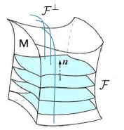
Figure 1: Local picture of the plaques of the foliations $\mathcal{F}$ and $\mathcal{F}^{\perp}$ inside some open subset of $M$.

3.3 Topological obstructions to existence of a nowhere-vanishing closed one-form in the cohomology class of $\mathbf{f}$

Notice that the cohomology class $\mathfrak{f}\in H^{1}(M,\mathbb{R})$ of $\mathbf{f}$ cannot be zero since otherwise the second condition in (40) would require that ${\boldsymbol{\omega}}=\mathrm{d}\alpha$ for some smooth map $\alpha:M\rightarrow\mathbb{R}$. Since $\alpha$ must attain its extrema on the compact manifold $M$, this would imply that ${\boldsymbol{\omega}}$ vanishes at those extrema, contradicting our requirement that $V$ (and thus also ${\boldsymbol{\omega}}$) be nowhere-vanishing. Thus $\mathfrak{f}$ must be a non-trivial cohomology class and hence the first Betti number of $M$ cannot be zero:

$$\boxed{b_{1}(M)>0}~{}~{}.$$ (41)

This condition is far from sufficient. To state further conditions on $\mathfrak{f}$, let us recall some facts regarding the period morphism of an element of $H^{1}(M,\mathbb{R})$.

The period morphism and period group of $\mathfrak{f}$.

Recall that integration of any representative of $\mathfrak{f}$ over closed paths provides a group morphism (called the period morphism) from the unbased first homotopy group to the additive group of the reals:

$$\mathrm{per}_{\mathfrak{f}}:\pi_{1}(M)\rightarrow\mathbb{R}~{}~{}.$$

This factors through the map $\pi_{1}(M)\stackrel{{\scriptstyle[~{}~{}]}}{{\rightarrow}}H_{1}^{\mathrm{tf}}(M,\mathbb{Z})$ which associates to each homotopy class $\alpha\in\pi_{1}(M)$ of a path its image $[\alpha]$ in the torsion-free part $H_{1}^{\mathrm{tf}}(M,\mathbb{Z})$ of $H_{1}(M,\mathbb{Z})$:

$$\mathrm{per}_{\mathfrak{f}}(\alpha)=\mathrm{per}^{\prime}_{\mathfrak{f}}([\alpha])~{}~{}.$$

The induced map $\mathrm{per}^{\prime}_{\mathfrak{f}}:H_{1}^{\mathrm{tf}}(M,\mathbb{Z})\rightarrow\mathbb{R}$ is called the reduced period morphism. The image $\Pi_{\mathfrak{f}}$ of $\mathrm{per}_{\mathfrak{f}}$ is a (necessarily free) Abelian subgroup of $\mathbb{R}$ called the group of periods of $\mathfrak{f}$ while the kernel $A_{\mathfrak{f}}$ of $\mathrm{per}_{\mathfrak{f}}$ is a normal subgroup of $\pi_{1}(M)$ called the $\mathfrak{f}$-irrelevant subgroup. It is obvious that $A_{\mathfrak{f}}$ contains the commutant subgroup $[\pi_{1}(M),\pi_{1}(M)]$. The corresponding subgroup $A^{\prime}_{\mathfrak{f}}=[A_{\mathfrak{f}}]=\ker(\mathrm{per}^{\prime}\mathfrak{f})$ of $H_{1}^{\mathrm{tf}}(M,\mathbb{Z})\subset H_{1}(M,\mathbb{Z})$ is called the $\mathfrak{f}$-irrelevant subgroup of the group of one-cycles.

The rank $\rho(\mathfrak{f})\stackrel{{\scriptstyle{\rm def.}}}{{=}}{\rm rk}\Pi_{\mathfrak{f}}$ of the period group is called the irrationality rank of $\mathfrak{f}$. We have $\rho(\mathfrak{f})=\dim_{\mathbb{Q}}\Pi_{\mathfrak{f}}$ if $\Pi_{\mathfrak{f}}$ is viewed as a finite-dimensional subspace of $\mathbb{R}$, when the latter is viewed as an infinite-dimensional vector space over the field $\mathbb{Q}$ of rational numbers. Notice that:

$$\boxed{\rho(\mathfrak{f})\leq b_{1}(M)}~{}~{}.$$ (42)

Let us assume that $\mathfrak{f}\neq 0$ (which, as explained above, is always the case in our application). Then $\Pi_{\mathfrak{f}}$ is a discrete subgroup of $(\mathbb{R},+)$ iff. $\rho(\mathfrak{f})=1$, in which case $\Pi_{\mathfrak{f}}$ is infinite-cyclic (hence isomorphic with $\mathbb{Z}$), i.e. we have $\Pi_{\mathfrak{f}}=\mathbb{Z}a_{\mathfrak{f}}$ where $a_{\mathfrak{f}}$ is the fundamental period of $\mathfrak{f}$, defined through:

$$a_{\mathfrak{f}}\stackrel{{\scriptstyle{\rm def.}}}{{=}}\inf(\Pi_{\mathfrak{f}}\cap\mathbb{N}^{\ast})>0~{}~{}.$$

Here $\mathbb{N}^{\ast}$ denotes the set $\mathbb{N}\setminus\{0\}$ of positive integers. This happens iff. there exists a positive real number $\lambda$ (for example, $\lambda=\frac{1}{a_{\mathfrak{f}}}$) such that $\lambda\mathfrak{f}\in H^{1}(M,\mathbb{Z})$ (equivalently, such that $\lambda\mathfrak{f}\in H^{1}(M,\mathbb{Q})$), in which case we say that $\mathfrak{f}$ is projectively rational. When $\rho(\mathfrak{f})>1$, the period group is a dense subgroup of $(\mathbb{R},+)$ and hence $\inf(\Pi_{\mathfrak{f}}\cap\mathbb{N}^{\ast})=0$. In this case we say that $\mathfrak{f}$ is projectively irrational.

Letting $b_{1}\stackrel{{\scriptstyle{\rm def.}}}{{=}}b_{1}(M)$ and picking a basis $c_{1},\ldots,c_{b_{1}}$ of the free Abelian group $H_{1}^{\mathrm{tf}}(M,\mathbb{Z})$, we have (in both cases mentioned above):

$$\Pi_{\mathfrak{f}}=\mathbb{Z}\mathrm{per}_{\mathfrak{f}}(c_{1})+\ldots+\mathbb{Z}\mathrm{per}_{\mathfrak{f}}(c_{b_{1}})\subset\mathbb{R}~{}~{}.$$

In the projectively rational case this sum equals $\Pi_{\mathfrak{f}}=\mathbb{Z}a_{\mathfrak{f}}$, since in that case we have $\mathrm{per}_{\mathfrak{f}}(c_{i})=\nu_{i}a_{\mathfrak{f}}$ for some (setwise) coprime integers $\nu_{1},\ldots,\nu_{b_{1}}$. For the general case, let $b_{1},\ldots,b_{\rho}\in\mathbb{R}$ (where $\rho\stackrel{{\scriptstyle{\rm def.}}}{{=}}\rho(\mathfrak{f})$) be a basis of the vector space $\mathbb{Q}\mathrm{per}_{\mathfrak{f}}(c_{1})+\ldots+\mathbb{Q}\mathrm{per}_{\mathfrak{f}}(c_{b_{1}})\subset\mathbb{R}$ generated by $\mathrm{per}_{\mathfrak{f}}(c_{i})$ over $\mathbb{Q}$. Then $\mathrm{per}_{\mathfrak{f}}(c_{i})=\sum_{k=1}^{\rho}q_{ik}b_{k}$ for some uniquely-determined rationals $q_{ik}$. Clearing denominators, we have $q_{ik}=q_{k}m_{ik}$ for some uniquely determined positive rationals $q_{k}$ and integers $m_{ik}$ such that $m_{1k},\ldots,m_{b_{1}k}$ are setwise coprime. Then $\Pi_{\mathfrak{f}}=\sum_{k=1}^{\rho}{\mathbb{Z}a_{k}}$, where the real numbers $a_{k}\stackrel{{\scriptstyle{\rm def.}}}{{=}}q_{k}b_{k}\in\mathbb{R}$ are rationally independent and thus they also form a basis of $\Pi_{\mathfrak{f}}$ over $\mathbb{Q}$. It follows that the last sum is direct, i.e.:

$$\Pi_{\mathfrak{f}}=\mathbb{Z}a_{1}\oplus\ldots\oplus\mathbb{Z}a_{\rho}~{}~{}.$$ (43)

This shows how one can find a basis of $\Pi_{\mathfrak{f}}$ when the latter is viewed as a free Abelian group.

The necessary and sufficient conditions.

Even on manifolds $M$ which satisfy (14) and (41), finding a nowhere-vanishing closed one-form lying in a cohomology class $\mathfrak{f}$ imposes further restrictions on that class and on the topology of $M$. The necessary and sufficient conditions are known Farrell ; Siebenmann ; Latour for manifolds $M$ of dimension greater than $5$ (which is our case). Since they are rather technical, we state them without giving any details, referring the reader to loc. cit. as well as to Schutz1 ; Schutz2 . Let $\hat{M}_{\mathfrak{f}}$ be the integration cover of $\mathrm{per}_{\mathfrak{f}}$, i.e. the Abelian regular covering space of $M$ corresponding to the normal subgroup $A_{\mathfrak{f}}$ of $\pi_{1}(M)$. When $\dim M\geq 6$, a class $\mathfrak{f}\in H^{1}(M,\mathbb{R})\setminus\{0\}$ contains a nowhere-vanishing closed one-form iff. $M$ is $(\pm\mathfrak{f})$-contractible and the Latour obstruction $\tau_{L}(M,\mathfrak{f})\in\mathrm{Wh}(\pi_{1}(M),\mathfrak{f})$ vanishes. Here $\mathrm{Wh}(\pi_{1}(M),\mathfrak{f})$ is the Whitehead group of the Novikov-Sikorav ring $\widehat{\mathbb{Z}\pi_{1}(M)}$ in the sense of Latour , the Novikov-Sikorav ring Sikorav (see also (Farber, , Subsection 3.1.5)) being a completion of the group ring $\mathbb{Z}\pi_{1}(M)$ with respect to a certain norm induced by the period morphism $\mathrm{per}_{\mathfrak{f}}$. When $\mathfrak{f}$ is a projectively rational class, these conditions are equivalent Ranicki with those found in Farrell ; Siebenmann , namely that the integration cover $\hat{M}_{\mathfrak{f}}$ (which in that case is infinite cyclic) must be finitely-dominated and that the Farrell-Siebenmann obstruction $\tau_{F}(M,\mathfrak{f})\in\mathrm{Wh}(\pi_{1}(M))$ must vanish, where $\mathrm{Wh}(\pi_{1}(M))$ is the Whitehead group of $\pi_{1}(M)$.

3.4 Solving the $\check{Q}$-constraints

Recall form ga1 that any inhomogeneous form decomposes uniquely as $\omega=\omega_{\perp}+{\hat{V}}\wedge\omega_{\top}$, where $\omega_{\perp}$ and $\omega_{\top}$ are orthogonal to ${\hat{V}}$ and thus belong to $\Omega(\mathcal{D})$. Since $\mathcal{F}$ carries a leafwise $G_{2}$ structure, we can parameterize $\omega_{\perp}$ and $\omega_{\top}$ for any pure rank form as recalled in Appendix B. In particular, we have $F=F_{\perp}+{\hat{V}}\wedge F_{\top}$ and $f=f_{\perp}+{\hat{V}}\wedge f_{\top}$, where $f_{\top}\in\Omega^{0}(M)$, $f_{\perp}\in\Omega^{1}(\mathcal{D})$, $F_{\top}\in\Omega^{3}(\mathcal{D})$ and $F_{\perp}\in\Omega^{4}(\mathcal{D})$. Relations (101), (102) of Appendix B give the parameterizations:

$$\boxed{\begin{split}&F_{\perp}=F_{\perp}^{(7)}+F_{\perp}^{(S)}~{}~{}\mathrm{where}~{}~{}F_{\perp}^{(7)}=\alpha_{1}\wedge\varphi\in\Omega^{4}_{7}(\mathcal{D})~{}~{},~{}~{}F_{\perp}^{(S)}=-\hat{h}_{kl}e^{k}\wedge\iota_{e^{l}}\psi\in\Omega^{4}_{S}(\mathcal{D})~{}~{}~{}\\ &F_{\top}=F_{\top}^{(7)}+F_{\top}^{(S)}~{}~{}\mathrm{where}~{}~{}F_{\top}^{(7)}=-\iota_{\alpha_{2}}\psi\in\Omega^{3}_{7}(\mathcal{D})~{}~{},~{}~{}F_{\top}^{(S)}=\chi_{kl}e^{k}\wedge\iota_{e^{l}}\varphi\in\Omega^{3}_{S}(\mathcal{D})~{}\end{split}}~{}~{}.~{}~{}~{}~{}~{}~{}~{}$$ (44)

Here $\alpha_{1},\alpha_{2}\in\Omega^{1}(\mathcal{D})$ and ${\hat{h}},\chi$ are leafwise covariant symmetric tensors, i.e. sections of the bundle $\mathrm{Sym}^{2}(\mathcal{D}^{\ast})$. Also recall from Appendix B that $F_{\top}^{(S)}=F_{\top}^{(1)}+F_{\top}^{(27)}$ with $F_{\top}^{(1)}\in\Omega^{3}_{1}(\mathcal{D})~{},~{}F_{\top}^{(27)}\in\Omega^{3}_{27}(\mathcal{D})$, with a similar decomposition for $F_{\perp}^{(S)}$. The last relations correspond to the decompositions of $\chi$ and ${\hat{h}}$ into their homothety and traceless parts $\chi^{(0)}$ and ${\hat{h}}^{(0)}$. Since $\psi=\ast_{\perp}\varphi=\ast_{\varphi}\varphi$ is determined by $\varphi$, relations (44) determine $F$ in terms of ${\hat{V}}$, $\psi$ and of the quantities $\alpha_{1},\alpha_{2},{\hat{h}}$ and $\chi$. The following result shows that the $\check{Q}$ constraints are equivalent with equations which determine $\alpha_{1},\alpha_{2}$ and $\mathrm{tr}_{g}({\hat{h}})$, $\mathrm{tr}_{g}(\chi)$ in terms of $\Delta$, $b$ and $f$.

Theorem 1.

Let $||V||=\sqrt{1-b^{2}}$. Then the $\check{Q}$-constraints (35) are equivalent with the following relations, which determine (in terms of $\Delta,b,{\hat{V}},\psi$ and $f$) the components of $F_{\top}^{(1)}$, $F_{\perp}^{(1)}$ and $F^{(7)}_{\top}$, $F_{\perp}^{(7)}$:

$$\boxed{\begin{split}&\alpha_{1}=\frac{1}{2||V||}(f-3b\mathrm{d}\Delta)_{\perp}~{},\\ &\alpha_{2}=-\frac{1}{2||V||}(bf-3\mathrm{d}\Delta)_{\perp}~{},\\ &\mathrm{tr}_{g}(\hat{h})=-\frac{3}{4}\mathrm{tr}_{g}(h)=\frac{1}{2||V||}(bf-3\mathrm{d}\Delta)_{\top}~{},\\ &\mathrm{tr}_{g}(\hat{\chi})=-\frac{3}{4}\mathrm{tr}_{g}(\chi)=3\kappa-\frac{1}{2||V||}(f-3b\mathrm{d}\Delta)_{\top}~{}.\end{split}}$$ (45)

Remark.

Notice that the $\check{Q}$-constraints (35) do not determine the components $F_{\top}^{(27)}$ and $F_{\perp}^{(27)}$.

Definition.

We say that a pair $(f,F)\in\Omega^{1}(M)\times\Omega^{4}(M)$ is consistent with a quadruple $(\Delta,b,{\hat{V}},\psi)$ if conditions (45) hold, i.e. if the $\check{Q}$-constraints are satisfied.

Proof. Writing $\check{E}=\frac{1}{16}(\alpha+\beta)$ and $\check{Q}=\frac{1}{12}(T-x)$, where:

$$\alpha\stackrel{{\scriptstyle{\rm def.}}}{{=}}V+Z=V(1+\psi)~{}\in\Omega^{\mathrm{odd}}(M)~{}~{},~{}~{}\beta\stackrel{{\scriptstyle{\rm def.}}}{{=}}1+Y+b\nu=(1+b\nu)(1+\psi)~{}\in\Omega^{\mathrm{ev}}(M)~{},$$

$$x\stackrel{{\scriptstyle{\rm def.}}}{{=}}F+12\kappa\nu~{}\in\Omega^{\mathrm{ev}}(M)~{}~{}~{}~{}~{}~{}~{}~{}~{}~{}~{}~{}~{}~{}~{},~{}~{}~{}T\stackrel{{\scriptstyle{\rm def.}}}{{=}}2(3\mathrm{d}\Delta-\ast f)~{}\in\Omega^{\mathrm{odd}}(M)$$

and using the fact that the geometric product is even with respect to the $\mathbb{Z}_{2}$-grading of $\Omega(M)$ given by the decomposition $\Omega(M)=\Omega^{\mathrm{ev}}(M)\oplus\Omega^{\mathrm{odd}}(M)$, the $\check{Q}$-constraints (35) can be brought to the form:

$$\big{[}xV-T(1+b\nu)\big{]}\Pi=0~{}~{},$$

$$\big{[}x(1+b\nu)-TV\big{]}\Pi=0~{}~{},$$ (46)

where (as mentioned before) the inhomogeneous form $\Pi\stackrel{{\scriptstyle{\rm def.}}}{{=}}\frac{1}{8}(1+\psi)$ is an idempotent in the Kähler-Atiyah algebra:

$$\Pi^{2}=\Pi~{}\Longleftrightarrow~{}(1+\psi)^{2}=8(1+\psi)~{}.$$

Since $\nu$ is twisted central in the Kähler-Atiyah algebra ga1 while $\iota_{V}\psi=0$, we have:

$$[\nu,\psi]_{-}=[V,\psi]_{-}=0~{}~{}\Longrightarrow~{}~{}[\nu,\Pi]_{-}=[V,\Pi]_{-}=0~{}~{}.$$

On the other hand, $V$ is invertible in the Kähler-Atiyah algebra, while $\nu$ is involutive ($\nu^{2}=1$). Using these observations, we compute:

$$V(1+b\nu)^{-1}=\frac{V(1-b\nu)}{||V||^{2}}=\frac{(1+b\nu)V}{||V||^{2}}~{}~{},~{}~{}\big{[}(1+b\nu)V\big{]}^{-1}=\frac{V(1-b\nu)}{||V||^{4}}$$

and find that the two equations of (3.4) (and thus the $\check{Q}$-constraints (35)) are both equivalent with the single condition:

$$\Big{[}x-\frac{T(1+b\nu)V}{||V||^{2}}\Big{]}\Pi=0~{}~{}.$$ (47)

Let

$$y\stackrel{{\scriptstyle{\rm def.}}}{{=}}\frac{T(1+b\nu)V}{||V||^{2}}=\frac{TV(1-b\nu)}{||V||^{2}}~{}~{}.$$

Separating (47) into components parallel and orthogonal to $V$, it becomes:

$$(x_{\parallel}-y_{\parallel})\Pi=(x_{\perp}-y_{\perp})\Pi=0~{}~{},$$ (48)

where:

$$y_{\parallel}=-\frac{1}{||V||}\big{[}{\hat{V}}\wedge T+b(\iota_{\hat{V}}T)\nu\big{]}~{}~{},~{}~{}y_{\perp}=\frac{1}{||V||}\big{[}\iota_{{}_{\hat{V}}}T+b({\hat{V}}\wedge T)\nu\big{]}~{}~{}.$$

Using the properties of Hodge duality, orthogonality and parallelism given in Appendix A, the system (48) is found to be equivalent with:

$$\Big{[}x_{\top}+\frac{1}{||V||}(T+bT\nu)_{\perp}\Big{]}\Pi=\Big{[}x_{\perp}-\frac{1}{||V||}(T+bT\nu)_{\top}\Big{]}\Pi=0~{}~{}.$$ (49)

Since $x_{\perp}=F_{\perp}$ while $x_{\top}=\iota_{{}_{{\hat{V}}}}x=F_{\top}+12\kappa\ast{\hat{V}}$, we find that (49) amounts to:

$$F_{\top}\Pi=-\frac{1}{||V||}\Big{[}(T+bT\nu)_{\perp}+12\kappa\ast V\Big{]}\Pi~{}~{},$$

$$F_{\perp}\Pi=\frac{1}{||V||}\iota_{{}_{{\hat{V}}}}(T+b\ast T)\Pi~{}~{}.$$

One computes:

$$T+b\ast T=2\big{[}3\mathrm{d}\Delta-bf+\nu(f-3b\mathrm{d}\Delta)\big{]}~{}~{},$$

so that the system finally becomes:

$$F_{\top}\Pi=-\frac{1}{||V||}\Big{[}2(3\mathrm{d}\Delta-bf)_{\perp}+2\big{[}6\kappa||V||-(f-3b\mathrm{d}\Delta)_{\top}\big{]}\nu_{{}_{\top}}\Big{]}\Pi~{},$$

$$F_{\perp}\Pi=\frac{1}{||V||}\Big{[}2(3\mathrm{d}\Delta-bf)_{\top}+2(f-3b\mathrm{d}\Delta)_{\perp}\nu_{{}_{\top}}\Big{]}\Pi~{}~{}.$$ (50)

Using the decomposition (44) of $F$ and the right action of $\psi$ (in the Kähler-Atiyah algebra) on 3- and 4-forms given in (113)-(114) of Appendix B, equations (3.4) reduce to:

$$F_{\top}(1+\psi)=-4\alpha_{2}+4F_{\top}^{(7)}+3\mathrm{tr}_{g}(\chi)\varphi-4\alpha_{2}\wedge\psi+3\mathrm{tr}_{g}(\chi)\nu_{\top}~{},$$

$$F_{\perp}(1+\psi)=-4\mathrm{tr}_{g}(\hat{h})+4\iota_{\alpha_{1}}\varphi+4F_{\perp}^{(7)}-4\mathrm{tr}_{g}(\hat{h})\psi+4\ast_{\perp}\alpha_{1}~{}~{}.$$ (51)

Identifying the terms of equal ranks, we find that (3.4) (and hence the $\check{Q}$-constraints (35)) are equivalent with relations (45) of the Theorem. $\blacksquare$

3.5 Extrinsic geometry of $\mathcal{F}$

As explained in Appendix C, the extrinsic geometry of $\mathcal{F}$ is described by the fundamental equations:

$$\boxed{\begin{split}&\nabla_{n}n=H~{}~{}~{}(\perp n)~{},\\ &\nabla_{X_{\perp}}n=-AX_{\perp}~{}~{}~{}(\perp n)~{},\\ &\nabla_{n}(X_{\perp})=-g(H,X_{\perp})n+D_{n}(X_{\perp})~{},\\ &\nabla_{X_{\perp}}(Y_{\perp})=\nabla^{\perp}_{X_{\perp}}(Y_{\perp})+g(AX_{\perp},Y_{\perp})n~{},\end{split}~{}~{}}$$ (52)

where $H\in\Gamma(M,\mathcal{D}^{\perp})$ encodes the second fundamental form of $\mathcal{F}^{\perp}$, $A\in\Gamma(M,\mathrm{End}(\mathcal{D}))$ is the Weingarten operator of the leaves of $\mathcal{F}$ and $D_{n}:\Gamma(M,\mathcal{D})\rightarrow\Gamma(M,\mathcal{D})$ is the derivative along the vector field $n$ taken with respect to the normal connection of the leaves of $\mathcal{F}^{\perp}$. The first and third relations are the Gauss and Weingarten equations for $\mathcal{F}^{\perp}$ while the second and fourth relations are the Weingarten and Gauss equations for $\mathcal{F}$. Notice that $D_{n}$ tells us how to transport tensors (co)tangent to the leaves of $\mathcal{F}$ in the direction orthogonal to its leaves, while preserving the metric induced on $\mathcal{D}=T\mathcal{F}=N(\mathcal{F}^{\perp})$. The O’Neill-Gray tensors ONeill ; Gray ; Tondeur of the foliation $\mathcal{F}$ can be expressed in terms of $H$ and $A$ through the relations:

$$\begin{split}&\mathcal{T}_{X}Y=\mathcal{T}_{X_{\perp}}Y\stackrel{{\scriptstyle{\rm def.}}}{{=}}(\nabla_{X_{\perp}}(Y_{\perp}))_{\parallel}+(\nabla_{X_{\perp}}(Y_{\parallel}))_{\perp}=[X_{\perp}(g(n,Y))+B(X_{\perp},Y_{\perp})]n+g(n,Y)H\\ &\mathcal{A}_{X}Y=\mathcal{A}_{X_{\parallel}}Y\stackrel{{\scriptstyle{\rm def.}}}{{=}}(\nabla_{X_{\parallel}}(Y_{\parallel}))_{\perp}+(\nabla_{X_{\parallel}}Y_{\perp})_{\parallel}=g(n,X)[-g(H,Y)n+g(n,Y)H]~{}~{},\end{split}$$ (53)

where:

$$B(X_{\perp},Y_{\perp})\stackrel{{\scriptstyle{\rm def.}}}{{=}}g(AX_{\perp},Y_{\perp})=B(Y_{\perp},X_{\perp})~{}~{}$$ (54)

is the scalar second fundamental form of $\mathcal{F}$ (see Appendix C). The Naveira tensor Naveira of the orthogonal almost product structure $\mathcal{P}$ defined by the pair of distributions $(\mathcal{D},\mathcal{D}^{\perp})$ can also be expressed in terms of $H$ and $A$ through the formulas given in Appendix C. Notice that $H$ and $A$ contain the same information as the O’Neill-Gray tensors/Naveira tensor and hence these quantities fully characterize the extrinsic geometry of $\mathcal{F}$. Let us examine some consequences of the fundamental equations (52).

The covariant derivatives of ${\hat{V}}$ and $V$.

The covariant derivative of the one-form ${\hat{V}}\in\Omega(\mathcal{D}^{\perp})$ (which is transverse to $\mathcal{F}$) can be computed using the relation ${\hat{V}}=n_{\sharp}$, which implies $(\nabla_{X}{\hat{V}})=(\nabla_{X}n)_{\sharp}$ for any vector field $X$ on $M$. Using the fundamental equations, we find:

$$\boxed{\nabla_{n}{\hat{V}}~{}~{}=H_{\sharp}~{}~{},~{}~{}\nabla_{X_{\perp}}{\hat{V}}=-(AX_{\perp})_{\sharp}}~{}~{}.$$ (55)

These relations imply:

$$\mathrm{d}{\hat{V}}={\hat{V}}\wedge H_{\sharp}~{}~{},~{}~{}\updelta{\hat{V}}=-\mathrm{tr}A~{}~{}.$$ (56)

Since $\iota_{\hat{V}}(H_{\sharp})=g(n,H)=0$, the first equation above gives $H_{\sharp}=(\mathrm{d}{\hat{V}})_{\top}=\iota_{\hat{V}}\mathrm{d}{\hat{V}}$. A simple computation now gives the following relations which express the covariant derivative of $V$:

$$\begin{split}&(\nabla_{n}V)_{\top}=\partial_{n}||V||~{}~{},~{}~{}(\nabla_{j}V)_{\top}=\partial_{j}||V||\\ &(\nabla_{n}V)_{\perp}=||V||H_{\sharp}~{}~{},~{}~{}(\nabla_{j}V)_{\perp}=-||V||(Ae_{j})_{\sharp}~{}~{}.\end{split}$$ (57)

Equations (57) give:

$$\mathrm{d}V={\hat{V}}\wedge(||V||H_{\sharp}-\mathrm{d}_{\perp}||V||)=V\wedge(H_{\sharp}-\mathrm{d}_{\perp}\ln||V||)~{}~{},~{}~{}\updelta V=-\partial_{n}||V||+||V||\mathrm{tr}A~{}~{}.$$ (58)

Remark.

Notice that the differential and codifferential (56) of ${\hat{V}}$ determine $H$ and $\mathrm{tr}A$ but they fail to determine the traceless part of $A$ and hence they do not fully determine the covariant derivative (55) of ${\hat{V}}$. If $H$ and $A$ are known, then the space of solutions of (55) is an affine space modeled on the kernel $\mathrm{\cal K}_{B}$ of the Bochner Laplacian $\nabla^{\ast}\nabla$ on $\Omega^{1}(M)$, thus $\mathrm{\cal K}_{B}$ is the space of parallel one-forms on $M$. On the other hand, the space of solutions of (56) is an affine space modeled on the kernel $\mathrm{\cal K}_{H}$ of the Hodge Laplacian $\mathrm{d}\updelta+\updelta\mathrm{d}$ on $\Omega^{1}(M)$, thus $\mathrm{\cal K}_{H}$ is the space of harmonic one-forms. Recall that the Bochner and Hodge Laplacians are related through the Weitzenbock identity:

$$\nabla^{\ast}\nabla=\mathrm{d}\updelta+\updelta\mathrm{d}+\mathcal{W}~{}~{},$$

where the Weitzenbock operator $\mathcal{W}$ depends on the Riemann curvature tensor of $g$. We have $\mathrm{\cal K}_{B}\subseteq\mathrm{\cal K}_{H}$, but, in general, the inclusion is strict. Hence, given $H$ and $A$, the space of solutions of (55) is generally smaller than the space of solutions to (56). Similar remarks of course also apply to $V$.

The covariant derivative, exterior derivative and codifferential of arbitrary forms decompose into components parallel and perpendicular to ${\hat{V}}$ according to the formulas given in Appendix C.

The normal covariant derivatives of $\varphi$ and $\psi$.

It is shown in Appendix C that the following relations hold:

$$\boxed{D_{n}\varphi=3\iota_{\vartheta}\psi~{}~{}~{},~{}~{}~{}D_{n}\psi=-3\vartheta\wedge\varphi}~{}~{}.$$ (59)

where $\vartheta\in\Omega^{1}(\mathcal{D})$ can be determined using the first relations in each of the two columns of (• ‣ B):

$$\vartheta=-\frac{1}{12}\ast_{\perp}[\varphi\wedge\ast_{\perp}(D_{n}\psi)]=-\frac{1}{12}\ast_{\perp}(\varphi\wedge D_{n}\varphi)~{}~{}.$$ (60)

3.6 Encoding the covariant derivative constraints through foliated geometry

In this Subsection, we prove the following result, which provides a solution to Problem 1 of Subsection 2.9:

Theorem 2.

Let $||V||=\sqrt{1-b^{2}}$ and suppose that $(F,f)$ is consistent with the quadruple $(\Delta,b,{\hat{V}},\psi)$, i.e. that the $\check{Q}$-constraints are satisfied. Then the covariant derivative constraints (34) are equivalent with the following conditions:

1. The function $b\in\mathcal{C}^{\infty}(M,(-1,1))$ satisfies:

   $$\boxed{e^{-3\Delta}\mathrm{d}(e^{3\Delta}b)=f-4\kappa\sqrt{1-b^{2}}{\hat{V}}}$$ (61)

2. The fundamental tensors $H$ and $A$ of $\mathcal{F}$ and $\mathcal{F}^{\perp}$ are given by the following expressions in terms of $b,\psi$ and $f,F$:

   $$\boxed{\begin{split}&H_{\sharp}=\frac{2}{||V||}\alpha_{2}=-\frac{1}{||V||^{2}}(bf-3\mathrm{d}\Delta)_{\perp}~{},\\ &AX_{\perp}=\frac{1}{||V||}\Big{[}(b\chi^{(0)}_{ij}-h^{(0)}_{ij})X_{\perp}^{j}e^{i}+\frac{1}{7}\big{(}14\kappa b-8\mathrm{tr}_{g}(\hat{h})-6b~{}\mathrm{tr}_{g}(\hat{\chi})\big{)}X_{\perp}\Big{]}=\\ &~{}~{}~{}~{}=\frac{1}{||V||}\Big{[}(b\chi^{(0)}_{ij}-h^{(0)}_{ij})X_{\perp}^{j}e^{i}+\frac{1}{7}\Big{(}-4\kappa b+9||V||(\mathrm{d}\Delta)_{\top}-\frac{1}{||V||}(bf-3\mathrm{d}\Delta)_{\top}\Big{)}X_{\perp}\Big{]}~{}~{},\end{split}}~{}~{}~{}~{}~{}~{}~{}~{}~{}$$ (62)

   i.e. the covariant derivative of ${\hat{V}}$ is given by (55), where $H$ and $A$ are given by (62).

3. The one-form $\vartheta\in\Omega(\mathcal{D})$ of (124) is given by the following relation in terms of $\Delta,b$ and $f$:

   $$\boxed{\vartheta=\frac{b\alpha_{2}-\alpha_{1}}{3||V||}=\frac{1}{6||V||^{2}}\big{[}-(1+b^{2})f+6b\mathrm{d}\Delta\big{]}_{\perp}}$$ (63)

4. The torsion classes of the leafwise $G_{2}$ structure (in the conventions of Bryant ; Kflows ) are given by the following expressions in terms of $\Delta,b$ and $f,F$:

   $$\boxed{\begin{split}&\boldsymbol{\tau}_{0}=\frac{4}{7||V||}(b~{}\mathrm{tr}_{g}(\hat{h})-\mathrm{tr}_{g}(\hat{\chi})+7\kappa)=\frac{4}{7||V||}\Big{[}4\kappa+\frac{(1+b^{2})f_{\top}-6b(\mathrm{d}\Delta)_{\top}}{2||V||}\Big{]}~{},\\ &\boldsymbol{\tau}_{1}=-\frac{3}{2}(\mathrm{d}\Delta)_{\perp}~{},\\ &\boldsymbol{\tau}_{2}=0~{},\\ &\boldsymbol{\tau}_{3}=\frac{1}{||V||}(\chi^{(0)}_{ij}-bh^{(0)}_{ij})e^{i}\wedge\iota_{e_{j}}\varphi=\frac{1}{||V||}(F_{\top}^{(27)}-b\ast_{\perp}F_{\perp}^{(27)})~{}.\end{split}}$$ (64)

   In particular, the leafwise $G_{2}$ structure is integrable (we have $\boldsymbol{\tau}_{2}=0$), i.e. it belongs to the class $W_{1}\oplus W_{3}\oplus W_{4}$ of the Fernandez-Gray classification FG .

Remarks.

1. Notice that Condition 2 of the theorem constrains the covariant derivative of ${\hat{V}}$ and not simply its exterior differential and codifferential (which are given by (56)). As remarked in Subsection 3.5, conditions (56) (with $H$ and $A$ given in (62)) are weaker than Condition 2 itself and hence they do not suffice to insure that the background is supersymmetric if $F$ and $f$ are fixed.

2. If $e_{a}$ is a local orthonormal frame of $M$ such that $e_{1}=n\stackrel{{\scriptstyle{\rm def.}}}{{=}}{\hat{V}}^{\sharp}$ and with dual coframe $e^{a}$ (thus $e^{a}={\hat{V}})$), then the second relation in (62) gives:

   $$B(e_{i},e_{j})\stackrel{{\scriptstyle{\rm def.}}}{{=}}g(e_{i},Ae_{j})=A_{ij}=\frac{1}{||V||}\big{(}-h^{(0)}_{ij}+b\chi^{(0)}_{ij}\big{)}+\frac{1}{7}\mathrm{tr}(A)g_{ij}~{},$$

   where:

   $$\mathrm{tr}A=\frac{1}{||V||}\big{(}14\kappa b-8\mathrm{tr}_{g}(\hat{h})-6b~{}\mathrm{tr}_{g}(\hat{\chi})\big{)}$$

   and, from (103), one has:

   $$h^{(0)}_{ij}=-\frac{1}{4}\left[\langle\iota_{e^{i}}\varphi,\iota_{e^{j}}(\ast_{\perp}F^{(27)})\rangle+(i\leftrightarrow j)\right]~{}~{},$$

   $$\chi^{(0)}_{ij}=-\frac{1}{4}\left[\langle\iota_{e^{i}}\varphi,\iota_{e^{j}}F^{(27)}\rangle+(i\leftrightarrow j)\right]~{}~{}.$$

   Notice that the Weingarten tensor $A$ is completely determined in terms of $F,f$ and $b$.

3. In general, neither $H$ nor $A$ (equivalently, $B$) vanish. Hence Reinhart’s criterion (see (Tondeur, , Theorem 5.17, p. 46)) tells us that, in general, neither $\mathcal{F}$ nor $\mathcal{F}^{\perp}$ are Riemannian foliations (i.e. $g$ is not a bundle-like metric for any of these foliations).

4. Since the leafwise $G_{2}$ structure has $\boldsymbol{\tau}_{2}=0$, the results of FriedrichIvanov1 insure existence of a unique metric but torsion-full leafwise partial connection $\nabla^{c}:\Gamma(M,\mathcal{D})\times\Gamma(M,\mathcal{D})\rightarrow\Gamma(M,\mathcal{D})$ which has ‘totally antisymmetric torsion tensor’ (corresponding through the musical isomorphism to a 3-form $T\in\Omega^{3}(\mathcal{D})$) and which is adapted to the $G_{2}$ structure:

   $$\nabla^{c}_{X_{\perp}}\varphi=0~{}~{},~{}~{}\forall X_{\perp}\in\Gamma(M,\mathcal{D})~{}~{}.$$

   Furthermore, the spinor $\eta_{0}$ of (29) satisfies $\nabla^{c}\eta_{0}=0$ (see FKMS ) and the torsion form $T$ and curvature of $\nabla^{c}$ can be computed using the formulas given in FriedrichIvanov1 ; FriedrichIvanov2 . Since $\boldsymbol{\tau}_{1}$ is exact, the leafwise $G_{2}$ structure is conformally co-calibrated (a.k.a. conformally co-closed). In fact, the conformal transformation (107) with $\alpha=\frac{3}{2}\Delta$ gives:

   $$\begin{split}&g^{\prime}_{ij}=e^{3\Delta}g_{ij}~{}~{}~{},~{}~{}\varphi^{\prime}=e^{\frac{9\Delta}{2}}\varphi~{}~{}~{}~{},~{}~{}~{}\psi^{\prime}=e^{6\Delta}\psi~{}~{},\\ &\boldsymbol{\tau}^{\prime}_{0}=e^{\frac{3\Delta}{2}}\boldsymbol{\tau}_{0}~{}~{}~{},~{}~{}\boldsymbol{\tau}^{\prime}_{1}=\boldsymbol{\tau}^{\prime}_{2}=0~{}~{},~{}~{}\boldsymbol{\tau}^{\prime}_{3}=e^{\frac{3\Delta}{2}}\boldsymbol{\tau}_{3}~{}~{},\end{split}$$

   so the conformally transformed $G_{2}$ structure satisfies $\mathrm{d}_{\perp}\psi^{\prime}=0$ i.e. $\updelta^{\prime}_{\perp}\varphi^{\prime}=0$. Co-calibrated $G_{2}$ structures were studied in GrigorianCoflow .

Proof of Theorem 2.

The rest of this Subsection is devoted to proving Theorem 2. We warn the reader that we give only the major steps of most computations and that performing some of the simplifications afforded by the $G_{2}$ structure identities of Appendix B is very tedious. We used the package Ricci Ricci for Mathematica^®, which we acknowledge here. Throughout the proof, we consider a local orthonormal frame of $M$ such that $e_{1}=n=\hat{V}^{\sharp}$.

Step 1. The covariant derivative constraints in the non-redundant parameterization.

Using the identities of Appendix (A) and (B), one can compute the explicit forms of $S_{m}^{(1)}$ and $S_{m}^{(8)}$, finding that the two equations of (3.1) which determine $\partial_{m}b$ and $\nabla_{m}V$ take the following form, in which $F$ was eliminated using the solution of the $\check{Q}$-constraints given in Theorem 1:

$$\begin{split}&\partial_{n}b=-\ast S_{1}^{(8)}=~{}||V||\Big{(}2\kappa-2\mathrm{tr}_{g}(\hat{\chi})\Big{)}~{},\\ &\partial_{j}b=-\ast S_{j}^{(8)}=~{}2||V||e_{j}\lrcorner\alpha_{1}~{},\end{split}$$ (65)

respectively:

$$\begin{split}&\nabla_{n}V=-S_{1}^{(1)}=2\alpha_{2}-\Big{(}2\kappa b-2b~{}\mathrm{tr}_{g}(\hat{\chi})\Big{)}\hat{V}~{},\\ &\nabla_{j}V=-S_{j}^{(1)}=\Big{[}h^{(0)}_{ij}-b\chi^{(0)}_{ij}-\frac{1}{7}\left(14\kappa b-8\mathrm{tr}_{g}(\hat{h})-6b~{}\mathrm{tr}_{g}(\hat{\chi})\right)g_{ij}\Big{]}e^{i}-2b(e_{j}\lrcorner\alpha_{1})\hat{V}~{}.\end{split}~{}~{}~{}~{}~{}~{}$$ (66)

In the non-redundant parameterization (31), one finds, after some computations, that the two equations of (3.1) which express $\nabla_{m}Y$ and $\nabla_{m}Z$ are equivalent with the relations:

$$\nabla_{m}\psi=-\frac{V}{||V||^{2}}[-S_{m}^{(1)}\psi+S_{m}^{(3)}+S_{m}^{(5)}]~{}~{},~{}~{}\nabla_{m}\psi=-\frac{V}{||V||^{2}}(1-b\nu)[S_{m}^{(4)}-S_{m}^{(8)}\psi]~{}~{},$$ (67)

which appear to impose the algebraic integrability condition:

$$-S_{m}^{(1)}\psi+S_{m}^{(3)}+S_{m}^{(5)}=(1-b\nu)[S_{m}^{(4)}-S_{m}^{(8)}\psi]~{}~{}.$$

A rather lengthy direct computation shows that this integrability condition is in fact automatically satisfied and thus provides no new conditions on the fluxes. Then (67) can be written in the equivalent form (D) given in Appendix D upon separating the parts orthogonal and parallel to $V$. Using the solution (44), (45) of the $Q$-constraints and the $G_{2}$ structure identities given in Appendix D, one finds after a lengthy computation that (D) simplifies to:

$$\begin{split}&(\nabla_{n}\psi)_{\top}=~{}-\frac{2}{||V||}\iota_{\alpha_{2}}\psi=\frac{1}{||V||^{2}}\iota_{(bf_{\perp}-3(\mathrm{d}\Delta)_{\perp})}\psi~{},\\ &(\nabla_{n}\psi)_{\perp}=\frac{\alpha_{1}-b\alpha_{2}}{||V||}\wedge\varphi=\frac{(1+b^{2})f_{\perp}-6b(\mathrm{d}\Delta)_{\perp}}{2||V||^{2}}\wedge\varphi~{},\\ &(\nabla_{j}\psi)_{\top}=\frac{1}{||V||}\Big{[}-h^{(0)}_{ij}+b\chi^{(0)}_{ij}+\frac{1}{7}\left(14\kappa b-8\mathrm{tr}_{g}(\hat{h})-6b~{}\mathrm{tr}_{g}(\hat{\chi})\right)g_{ij}\Big{]}\iota_{e_{i}}\psi~{},\\ &(\nabla_{j}\psi)_{\perp}=\frac{3}{2}(\mathrm{d}\Delta)_{\perp}\wedge\iota_{e^{j}}\psi-\frac{3}{2}e^{j}\wedge\iota_{(\mathrm{d}\Delta)_{\perp}}\psi-\frac{1}{||V||}\Big{[}bh^{(0)}_{ij}-\chi^{(0)}_{ij}+\frac{1}{7}\left(b~{}\mathrm{tr}_{g}(\hat{h})-\mathrm{tr}_{g}(\hat{\chi})+7\kappa\right)g_{ij}\Big{]}e^{i}\wedge\varphi~{}.\end{split}$$ (68)

In conclusion, the covariant derivative constraints (34) are equivalent, modulo the $\check{Q}$-constraints, with equations (65), (66) and (68). Direct computation using the first and last relation in (45) shows that the system (65) is equivalent with relation (61).

Remark.

Using these equations, one can also compute the covariant derivative of $\varphi$ and the explicit form of the exterior differential and codifferential constraints (38) and (39), which are given in Appendix D.

Step 2. Extracting $H$ and $A$.

Lemma.

Assume that $||V||^{2}=1-b^{2}$. Then:

1. The second equation on the first row of (3.1) (the covariant derivative constraint for $V$) is equivalent with the following relations:

$$H_{\sharp}=-\frac{1}{||V||}[S_{1}^{(1)}]_{\perp}~{}~{},~{}~{}(Ae_{j})_{\sharp}=\frac{1}{||V||}[S^{(1)}_{j}]_{\perp}~{}~{},~{}~{}\frac{b\partial_{m}b}{||V||}=[S^{(1)}_{m}]_{\top}~{}~{}.$$ (69)

2. Modulo the first equation in (3.1) (i.e. the covariant differential constraints for $b$), the last relation in (69) is equivalent with the following algebraic condition for $S^{(1)}$ and $S^{(8)}$:

$$[S_{m}^{(1)}]_{\top}=-\frac{b}{||V||}\ast S_{m}^{(8)}~{}~{}.$$ (70)

3. Condition (70) is automatically satisfied when $S_{m}^{(1)}$ and $S_{m}^{(8)}$ are given by expressions (65) and (66). Furthermore, the first two equations in (69) take the form (62) when substituting these expressions for $S_{m}^{(1)}$ and $S_{m}^{(8)}$. Hence the first row of (3.1) is equivalent, modulo the $\check{Q}$-constraints, with the first two equations in (62) and the first equation in (3.1), which in turn is equivalent with (65) and with (61).

Proof. The first statement follows by separating the ‘top‘ and ‘perp‘ parts of the covariant derivative constraint for $V$ given in (3.1) and comparing with (57) while using the relation $\partial_{m}||V||=-\frac{b\partial_{m}b}{||V||}$, which is implied by the condition $||V||^{2}=1-b^{2}$. The second statement now follows upon eliminating $\partial_{m}b$ from the third relation in (69) by using the differential constraint for $b$ given in (3.1). The remaining statements of the lemma follow by direct computation. $\blacksquare$

Step 3. Extracting the normal and longitudinal covariant derivatives of $\psi$.

Applying (C.2) for $\omega=\psi$, we find the following:

• The first and third equation of (C.2) for $\omega=\psi$ are equivalent respectively with the first and third equation of (68) upon using expressions (62) for $H$ and $A$.

• The second equation of (C.2) for $\omega=\psi$ agrees with the second equation of (68) provided that the normal covariant derivative of $\psi$ is given by:

  $$D_{n}\psi=~{}\frac{\alpha_{1}-b\alpha_{2}}{||V||}\wedge\varphi~{}~{}.$$ (71)

  Relation (71) determines the one-form $\vartheta$ of (124). Comparing with the second equation of (59) gives (63).

• The last equation of (C.2) for $\omega=\psi$ agrees with the second equation of (68) provided that the induced covariant derivative of $\psi$ along the leaves of the foliation is given by: ​​​​​​​​​​​​​​​​​​​​​​​​

  $$\!\!\!\!\!\!\!\!\!\!\!\!\nabla_{j}^{\perp}\psi=\frac{3}{2}(\mathrm{d}\Delta)_{\perp}\wedge\iota_{e^{j}}\psi-\frac{3}{2}e^{j}\wedge\iota_{(\mathrm{d}\Delta)_{\perp}}\psi-\frac{1}{||V||}\Big{[}bh^{(0)}_{ij}-\chi^{(0)}_{ij}+\frac{1}{7}\left(b~{}\mathrm{tr}_{g}(\hat{h})-\mathrm{tr}_{g}(\hat{\chi})+7\kappa\right)g_{ij}\Big{]}e^{i}\wedge\varphi~{}.~{}~{}~{}~{}~{}~{}~{}~{}~{}~{}~{}~{}$$ (72)

Hence the entire system (68) of covariant derivative constraints for $\psi$ is equivalent with equations (62) taken together with (71) and (72).

Step 4. Encoding the longitudinal covariant derivative of $\psi$ through the torsion forms of the leafwise $G_{2}$-structure.

Relation (72) can be expressed in a simpler equivalent form using the fact FG that the covariant derivative of the associative and/or coassociative forms of a manifold with $G_{2}$ structure (taken with respect to the Levi-Civita connection of the corresponding metric) is completely specified by the torsion classes of that $G_{2}$ structure. The torsion forms $\boldsymbol{\tau}_{0}\in\Omega^{0}_{1}(\mathcal{D})$, $\boldsymbol{\tau}_{1}\in\Omega^{1}_{7}(\mathcal{D})$, $\boldsymbol{\tau}_{2}\in\Omega^{2}_{14}(\mathcal{D})$ and $\boldsymbol{\tau}_{3}\in\Omega^{3}_{27}(\mathcal{D})$ of the leafwise $G_{2}$ structure (in the conventions of Bryant ; Kflows ) are uniquely determined by relations (104) and hence can be extracted by computing the differentials of $\psi$ and $\varphi$ starting from equation (72), which gives:

$$\mathrm{d}_{\perp}\psi=e^{j}\wedge(\nabla_{j}\psi)_{\perp}=-6(\mathrm{d}\Delta)_{\perp}\wedge\psi~{}~{},$$

and:

$$\mathrm{d}_{\perp}\varphi = e^{j}\wedge(\nabla_{j}\varphi)_{\perp}=-\ast_{\perp}[\iota_{e^{j}}(\nabla_{j}\psi)_{\perp}]=\ast_{\perp}\updelta_{\perp}\psi=$$

$$= -\frac{9}{2}(\mathrm{d}\Delta)_{\perp}\wedge\varphi+\frac{4}{7||V||}\left(b~{}\mathrm{tr}(\hat{h})-\mathrm{tr}_{g}(\hat{\chi})+7\kappa\right)\psi+\frac{1}{||V||}\ast_{\perp}(F_{\top}^{(27)}-b\ast F_{\perp}^{(27)})~{}.$$

Comparing with (104) gives relations (64). The results of FG assure us that equation (72) is equivalent with conditions (104), where the torsion classes are given by (64). Theorem 2 now follows by combining the previous statements. $\blacksquare$

3.7 The exterior derivatives of $\varphi$ and $\psi$ and the differential and codifferential of $V$

Applying (119) to the longitudinal forms $\varphi\in\Omega^{3}(\mathcal{D})$ and $\psi\in\Omega^{4}(\mathcal{D})$ gives:

$$(\mathrm{d}\varphi)_{\top}=D_{n}\varphi-A_{jk}e^{j}\wedge\iota_{e^{k}}\varphi~{}~{},~{}~{}~{}(\mathrm{d}\varphi)_{\perp}=\mathrm{d}_{\perp}\varphi=\boldsymbol{\tau}_{0}\psi+3\boldsymbol{\tau}_{1}\wedge\varphi+\ast_{\perp}\boldsymbol{\tau}_{3}~{}~{},$$

$$(\mathrm{d}\psi)_{\top}=D_{n}\psi-A_{jk}e^{j}\wedge\iota_{e^{k}}\psi~{}~{},~{}~{}~{}(\mathrm{d}\psi)_{\perp}=\mathrm{d}_{\perp}\psi=4\boldsymbol{\tau}_{1}\wedge\psi+\ast_{\perp}\boldsymbol{\tau}_{2}~{}~{}.$$ (73)

The second relations in each row above show that $(\mathrm{d}\varphi)_{\perp}$ and $(\mathrm{d}\psi)_{\perp}$ determine the torsion classes of the leafwise $G_{2}$ structure. Decomposing the first relation in each row according to the irreducible components of the $G_{2}$ action on $\wedge^{3}\mathcal{D}^{\ast}$ and $\wedge^{4}\mathcal{D}^{\ast}$, we find:

$$(\mathrm{d}\varphi)_{\top}^{(1)}=-\frac{3}{7}(\mathrm{tr}A)\varphi~{}~{},~{}~{}(\mathrm{d}\varphi)^{(7)}_{\top}=D_{n}\varphi~{}~{},~{}~{}(\mathrm{d}\varphi)^{(27)}_{\top}=-A_{jk}^{(0)}e^{j}\wedge\iota_{e^{k}}\varphi~{}~{},$$

$$(\mathrm{d}\psi)_{\top}^{(1)}=-\frac{4}{7}(\mathrm{tr}A)\psi~{}~{},~{}~{}(\mathrm{d}\psi)^{(7)}_{\top}=D_{n}\psi~{}~{},~{}~{}(\mathrm{d}\psi)^{(27)}_{\top}=-A_{jk}^{(0)}e^{j}\wedge\iota_{e^{k}}\psi~{}~{}.$$ (74)

which shows that any of $(\mathrm{d}\varphi)_{\top}$ or $(\mathrm{d}\psi)_{\top}$ suffices to determine the Weingarten tensor $A$ as well as $\vartheta$.

Remark.

One might imagine that the remark above obsoletes the need for the analysis of the full covariant derivatives which we carried out in the proof of Theorem 2 — since the differential and codifferential of $\varphi$ and $\psi$ determine $A,\vartheta$ and the torsion classes of the leafwise $G_{2}$ structure, while the differential of ${\hat{V}}$ determines $H$ (see (56)), one might be tempted to think that one could use them from the outset and forget about the full covariant derivatives of $\varphi$ and $\psi$. This, however, would be insufficient to prove a result such as Theorem 2, since it is not clear a priori that there are no supplementary algebraic constraints imposed by the full supersymmetry conditions (34) and (35). The point of Theorem 2 is that it gives an equivalent geometric characterization of the supersymmetry conditions, without loosing any information contained in the latter. Notice also that the supersymmetry conditions determine the covariant derivative (57) of $V$ if $f$ and $F$ are given (since they determine $H$ and $A$ as well as $\partial_{m}b$). This is stronger than simply determining the differential and codifferential of $V$. In fact, the covariant derivatives:

$$\nabla_{n}V = 2\alpha_{2}+2b\big{(}\mathrm{tr}_{g}(\hat{\chi})-\kappa\big{)}\hat{V}~{},$$ (75)

$$\nabla_{j}V = -2b(e_{j}\lrcorner\alpha_{1})\hat{V}+\Big{[}h^{(0)}_{ij}-b\chi^{(0)}_{ij}-\frac{1}{7}\big{(}14\kappa b-8\mathrm{tr}_{g}(\hat{h})-6b~{}\mathrm{tr}_{g}(\hat{\chi})\big{)}g_{ij}\Big{]}e^{i}~{}$$

depend explicitly on the fluxes $f$ and $F$ (through the tensors $\hat{h},\hat{\chi}$) while the differential and codifferential of $V$:

$$\mathrm{d}V = 3V\wedge(\mathrm{d}\Delta)_{\perp}~{},$$

$$\updelta V = -8\kappa b+12||V||(\mathrm{d}\Delta)_{\top}~{}~{}$$ (76)

depend only on $b$ (equivalently, on $||V||)$ and on $\Delta$ and $n$.

3.8 Eliminating the fluxes

The following result gives the set of conditions equivalent with the existence of at least one non-trivial solution $\xi$ of (4) which is everywhere non-chiral, while expressing $f$ and $F$ in terms of $\Delta$ and of the quantities $b,{\hat{V}}$ and $\varphi$ of (33). This solves Problem 2 of Subsection 2.9.

Theorem 3.

The following statements are equivalent:

1. There exist $f\in\Omega^{1}(M)$ and $F\in\Omega^{4}(M)$ such that (4) admits at least one non-trivial solution $\xi$ which is everywhere non-chiral (and which we can take to be everywhere of norm one).

2. There exist $\Delta\in{{\cal\mathcal{C}}^{\infty}(M,\mathbb{R})}$, $b\in\mathcal{C}^{\infty}(M,(-1,1))$, ${\hat{V}}\in\Omega^{1}(M)$ and $\varphi\in\Omega^{3}(M)$ such that:

   1. $\Delta$, $b$, ${\hat{V}}$ and $\varphi$ satisfy the conditions:

      $$||{\hat{V}}||=1~{}~{},~{}~{}\iota_{\hat{V}}\varphi=0~{}~{}.$$ (77)

      Furthermore, the Frobenius distribution $\mathcal{D}\stackrel{{\scriptstyle{\rm def.}}}{{=}}\ker{\hat{V}}$ is integrable and we let $\mathcal{F}$ be the foliation which integrates it.

   2. The quantities $H$, $\mathrm{tr}A$ and $\vartheta$ of the foliation $\mathcal{F}$ are given by:

      $$\boxed{\begin{split}&H_{\sharp}=\frac{2}{||V||}\alpha_{2}=-\frac{b}{||V||^{2}}(\mathrm{d}b)_{\perp}+3(\mathrm{d}\Delta)_{\perp}=\frac{\mathrm{d}_{\perp}||V||}{||V||}+3(\mathrm{d}\Delta)_{\perp}~{},\\ &\mathrm{tr}A=12(\mathrm{d}\Delta)_{\top}-\frac{b(\mathrm{d}b)_{\top}}{||V||^{2}}-8\kappa\frac{b}{||V||}=12\partial_{n}\Delta+\frac{\partial_{n}||V||-8\kappa b}{||V||}~{},\\ &\vartheta=-\frac{1+b^{2}}{6||V||^{2}}(\mathrm{d}b)_{\perp}+\frac{b}{2}(\mathrm{d}\Delta)_{\perp}~{}~{}.\end{split}}$$ (78)

   3. $\varphi$ induces a leafwise $G_{2}$ structure on $\mathcal{F}$ whose torsion classes satisfy:

      $$\boxed{\begin{split}&\boldsymbol{\tau}_{0}=\frac{4}{7||V||}\Big{[}2\kappa(3+b^{2})-\frac{3b}{2}||V||(\mathrm{d}\Delta)_{\top}+\frac{1+b^{2}}{2||V||}(\mathrm{d}b)_{\top}\Big{]}~{},\\ &\boldsymbol{\tau}_{1}=-\frac{3}{2}(\mathrm{d}\Delta)_{\perp}~{},\\ &\boldsymbol{\tau}_{2}=0~{}~{}.\end{split}}$$ (79)

In this case, the forms $f$ and $F$ are uniquely determined by $b,\Delta,V$ and $\varphi$. Namely, the one-form $f$ is given by:

$$\boxed{f=4\kappa V+e^{-3\Delta}\mathrm{d}(e^{3\Delta}b)}~{}~{},$$ (80)

while $F$ is given as follows:

1. We have $F^{(1)}_{\top}=\frac{3}{7}\mathrm{tr}_{g}(\chi)\varphi=-\frac{4}{7}\mathrm{tr}_{g}(\hat{\chi})\varphi$ and $F^{(1)}_{\perp}=-\frac{4}{7}\mathrm{tr}_{g}(\hat{h})\psi$, with:

   $$\boxed{\mathrm{tr}_{g}(\hat{h})=-\frac{3||V||}{2}(\mathrm{d}\Delta)_{\top}+2\kappa b+\frac{b}{2||V||}(\mathrm{d}b)_{\top}~{}~{}~{},~{}~{}~{}\mathrm{tr}_{g}(\hat{\chi})=\kappa-\frac{1}{2||V||}(\mathrm{d}b)_{\top}}$$ (81)

2. We have $F^{(7)}_{\top}=-\iota_{\alpha_{2}}\psi$ and $F^{(7)}_{\perp}=\alpha_{1}\wedge\varphi$, with:

   $$\boxed{\alpha_{1}=\frac{1}{2||V||}(\mathrm{d}b)_{\perp}~{}~{}~{},~{}~{}~{}\alpha_{2}=-\frac{b}{2||V||}(\mathrm{d}b)_{\perp}+\frac{3||V||}{2}(\mathrm{d}\Delta)_{\perp}=\frac{\mathrm{d}_{\perp}||V||}{||V||}+\frac{3||V||}{2}(\mathrm{d}\Delta)_{\perp}}~{}~{}~{}$$ (82)

3. We have:

   $$\boxed{\begin{split}h^{(0)}_{ij}=-\frac{b}{4||V||}[\langle e_{i}\lrcorner\varphi,e_{j}\lrcorner\boldsymbol{\tau}_{3}\rangle+(i\leftrightarrow j)]-\frac{1}{||V||}A^{(0)}_{ij}=\frac{b}{||V||}t_{ij}-\frac{1}{||V||}A^{(0)}_{ij}~{}~{},\\ \chi^{(0)}_{ij}=-\frac{1}{4||V||}[\langle e_{i}\lrcorner\varphi,e_{j}\lrcorner\boldsymbol{\tau}_{3}\rangle+(i\leftrightarrow j)]-\frac{b}{||V||}A^{(0)}_{ij}=\frac{1}{||V||}t_{ij}-\frac{b}{||V||}A^{(0)}_{ij}~{}~{},\end{split}}$$

   (where in the last equalities we used relation (106)), i.e.:

   $$F^{(27)}_{\perp}=-h^{(0)}_{ij}e^{i}\wedge\iota_{e^{j}}\psi=\frac{b}{||V||}\ast_{\perp}\boldsymbol{\tau}_{3}+\frac{1}{||V||}A^{(0)}_{ij}e^{i}\wedge\iota_{e^{j}}\psi~{}~{},$$

   $$F^{(27)}_{\top}=\chi^{(0)}_{ij}e^{i}\wedge\iota_{e^{j}}\varphi=\frac{1}{||V||}\boldsymbol{\tau}_{3}-\frac{b}{||V||}A^{(0)}_{ij}e^{i}\wedge\iota_{e^{j}}\varphi~{}~{},$$ (83)

   where $A^{(0)}$ is the traceless part of the Weingarten tensor of $\mathcal{F}$ while $\boldsymbol{\tau}_{3}$ is the rank 3 torsion class of the leafwise $G_{2}$ structure.

Remarks.

1. We show in Appendix D that (81) and (82) are equivalent with (MartelliSparks, , eqs. (3.20), (3.21)). Notice that loc. cit. does not give the component $F^{(27)}$, which we give here explicitly (see relation (c)).

2. Using (58) as well as the identities:

   $$e^{-3\Delta}\mathrm{d}(e^{3\Delta}V)=\mathrm{d}V-3V\wedge\mathrm{d}\Delta~{}~{},~{}~{}e^{-12\Delta}\updelta(e^{12\Delta}V)=\updelta V-12||V||\partial_{n}\Delta~{}~{},$$

   it is easy to check that the first and second conditions in (78) are equivalent with the following two equations for $V$:

   $$\boxed{\begin{split}&&\mathrm{d}(e^{3\Delta}V)=0\\ &&e^{-12\Delta}\updelta(e^{12\Delta}V)+8\kappa b=0\end{split}}~{}~{},$$ (84)

   where the second equation in (84) can also be written as follows upon using an orthonormal frame with $e_{1}=n$:

   $$e^{-12\Delta}\partial_{n}(e^{12\Delta}\sqrt{1-b^{2}})=8\kappa b~{}~{}.$$

   Since the first relation in (84) implies integrability of $\mathcal{D}$, it follows that this condition stated in point (B.1) of the theorem is in fact implied by the conditions stated in point (B.2). It turns out that conditions (84) coincide with (Tsimpis, , eqs. (3.16)), since it is possible to show that the quantity denoted by $L$ in loc. cit. is given by $L=\frac{1}{1+b}V$.

3. The theorem allows one to determine the metric $g$ as follows. First notice that (84) can be written as:

   $$\begin{split}&-\partial_{n}||V||+8\kappa b=12||V||\partial_{n}\Delta~{}~{},\\ &-\frac{\mathrm{d}_{\perp}||V||}{||V||}=3(\mathrm{d}\Delta)_{\perp}-n\lrcorner\mathrm{d}{\hat{V}}~{}~{}.\end{split}$$ (85)

   If $n$ and $\mathcal{D}$ are given, then ${\hat{V}}$ is uniquely determined by the conditions:

   $$\ker{\hat{V}}=\mathcal{D}~{}~{},~{}~{}n\lrcorner{\hat{V}}=1$$ (86)

   and (LABEL:beq) can be used to determine $\Delta$ if $b$ is given or to determine $b$ if $\Delta$ is given. Now suppose that $\Delta$, $\mathcal{F}$, $n$ and a leafwise $G_{2}$ structure along $\mathcal{F}$ are given, where $n$ is a vector field on $M$ which is everywhere transverse to $\mathcal{F}$ and where the torsion classes of the leafwise $G_{2}$ structure satisfy (79). Then $\mathcal{D}=T\mathcal{F}$ and ${\hat{V}}$ is determined by (86). The system (LABEL:beq) can be used to determine $b$ and hence $||V||^{2}$ and $V$, which in turn fixes the restriction of the metric $g$ to the foliation $\mathcal{F}^{\perp}$ which integrates the vector field $n$. The restriction of the metric on $\mathcal{F}$ (and hence the metric on $M$) is then determined by the associative form $\varphi$ of the leafwise $G_{2}$ structure through relation (23). Using these observations, one can formulate the mathematical problem of studying our backgrounds in a metric-free manner, namely as a problem of foliations which can be defined by a closed one form and which are endowed with longitudinal $G_{2}$ structures satisfying the version of the conditions listed in point 3 of the theorem which is obtained by expressing $b$ as the solution of (LABEL:beq). This approach could be used to construct examples of such foliations.

Proof.

Using relations (65), we extract $\alpha_{1}$ and $\mathrm{tr}_{g}(\hat{\chi})$:

$$\alpha_{1}=\frac{1}{2||V||}(\mathrm{d}b)_{\perp}~{}~{}~{},~{}~{}~{}\mathrm{tr}_{g}(\hat{\chi})=\kappa-\frac{1}{2||V||}(\mathrm{d}b)_{\top}~{}~{}.$$ (87)

Substituting these relations into the first and fourth relations of (45), we find the following expressions for the components of the 1-form flux:

$$f_{\perp}=(\mathrm{d}b)_{\perp}+3b(\mathrm{d}\Delta)_{\perp}~{},$$

$$f_{\top}=3b(\mathrm{d}\Delta)_{\top}+(\mathrm{d}b)_{\top}+4\kappa||V||~{}.$$ (88)

The second and third relations in (45) become:

$$\alpha_{2}=-\frac{b}{2||V||}(\mathrm{d}b)_{\perp}+\frac{3||V||}{2}(\mathrm{d}\Delta)_{\perp}~{},$$

$$\mathrm{tr}_{g}(\hat{h})=-\frac{3||V||}{2}(\mathrm{d}\Delta)_{\top}+2\kappa b+\frac{b}{2||V||}(\mathrm{d}b)_{\top}~{}.$$ (89)

Substituting (3.8) and (3.8) into (62) gives:

$$H_{\sharp}=\frac{2}{||V||}\alpha_{2}=-\frac{b}{||V||^{2}}(\mathrm{d}b)_{\perp}+3(\mathrm{d}\Delta)_{\perp}~{}~{},$$ (90)

$$B(e_{i},e_{j})\stackrel{{\scriptstyle{\rm def.}}}{{=}}g(e_{i},Ae_{j})=A_{ij}=\frac{1}{||V||}(b\chi^{(0)}_{ij}-h^{(0)}_{ij})+\frac{1}{7}\Big{[}12(\mathrm{d}\Delta)_{\top}-\frac{b(\mathrm{d}b)_{\top}}{||V||^{2}}-\frac{8\kappa b}{||V||}\Big{]}g_{ij}~{}~{},$$

where the traceless symmetric tensors can be expressed from relations (c) and (103) as follows:

$$h^{(0)}_{ij} = -\frac{1}{4}\left[\langle\iota_{e^{i}}\varphi,\iota_{e^{j}}(\ast_{\perp}F^{(27)}_{\perp})\rangle+(i\leftrightarrow j)\right]=-\frac{b}{4||V||}\left[\langle\iota_{e^{i}}\varphi,\iota_{e^{j}}\boldsymbol{\tau}_{3}\rangle+(i\leftrightarrow j)\right]-\frac{1}{||V||}A^{(0)}_{ij}~{},$$

$$\chi^{(0)}_{ij} = -\frac{1}{4}\left[\langle\iota_{e^{i}}\varphi,\iota_{e^{j}}F^{(27)}_{\top}\rangle+(i\leftrightarrow j)\right]=-\frac{1}{4||V||}\left[\langle\iota_{e^{i}}\varphi,\iota_{e^{j}}\boldsymbol{\tau}_{3}\rangle+(i\leftrightarrow j)\right]-\frac{b}{||V||}A^{(0)}_{ij}~{}.$$ (91)

Using (87), (3.8) and (3.8), the covariant derivatives (68) and (D) of $\psi$ become:

$$(\nabla_{n}\psi)_{\top}=~{}-\frac{2}{||V||}\iota_{\alpha_{2}}\psi=\frac{b}{||V||^{2}}\iota_{(\mathrm{d}b)_{\perp}}\psi-3\iota_{(\mathrm{d}\Delta)_{\perp}}\psi~{},$$

$$(\nabla_{n}\psi)_{\perp}=\frac{\alpha_{1}-b\alpha_{2}}{||V||}\wedge\varphi=\Big{[}\frac{(1+b^{2})}{2||V||^{2}}(\mathrm{d}b)_{\perp}-\frac{3b}{2}(\mathrm{d}\Delta)_{\perp}\Big{]}\wedge\varphi~{},$$ (92)

$$(\nabla_{j}\psi)_{\top}=\frac{1}{||V||}\Big{[}-h^{(0)}_{ij}+b\chi^{(0)}_{ij}+\frac{1}{7}\Big{(}12||V||(\mathrm{d}\Delta)_{\top}-8\kappa b-\frac{b}{||V||}(\mathrm{d}b)_{\top}\Big{)}g_{ij}\Big{]}\iota_{e_{i}}\psi~{},$$

$$(\nabla_{j}\psi)_{\perp}=\frac{3}{2}(\mathrm{d}\Delta)_{\perp}\wedge\iota_{e^{j}}\psi-\frac{3}{2}e^{j}\wedge\iota_{(\mathrm{d}\Delta)_{\perp}}\psi-\frac{1}{||V||}(bh^{(0)}_{ij}-\chi^{(0)}_{ij})e^{i}\wedge\varphi$$

$$~{}~{}~{}~{}~{}~{}~{}~{}~{}~{}~{}-\frac{1}{7||V||}\big{[}2\kappa(3+b^{2})-\frac{3b}{2}||V||(\mathrm{d}\Delta)_{\top}+\frac{1+b^{2}}{2||V||}(\mathrm{d}b)_{\top}\big{]}e^{j}\wedge\varphi~{}.$$

These expressions allow us to compute:

$$\mathrm{d}_{\perp}\psi=e^{j}\wedge(\nabla_{j}\psi)_{\perp}=6(\mathrm{d}\Delta)_{\perp}\wedge\psi~{},$$

$$\mathrm{d}_{\perp}\varphi=e^{j}\wedge\ast_{\perp}(\nabla_{j}\psi)_{\perp}=-\frac{9}{2}(\mathrm{d}\Delta)_{\perp}\wedge\varphi+\frac{4}{7||V||}\Big{[}2\kappa(3+b^{2})-\frac{3b}{2}||V||(\mathrm{d}\Delta)_{\top}+\frac{1+b^{2}}{2||V||}(\mathrm{d}b)_{\top}\Big{]}\psi$$

$$~{}~{}~{}~{}~{}~{}~{}~{}~{}~{}~{}~{}~{}~{}~{}~{}~{}~{}~{}~{}~{}~{}~{}~{}~{}~{}~{}~{}~{}~{}~{}+\frac{1}{||V||}\ast_{\perp}(F^{(27)}_{\top}-b\ast_{\perp}F^{(27)}_{\perp})~{}.$$

Comparing with (104) gives (79). Finally, notice that the second relation in (62) can be written as:

$$e^{j}\wedge(\nabla_{j}\varphi)_{\top}=e^{j}\wedge\iota_{Ae_{j}}\varphi=\frac{1}{||V||}\Big{[}-\ast_{\perp}F^{(27)}_{\perp}+bF^{(27)}_{\top}+\frac{3}{7}\Big{(}12||V||(\mathrm{d}\Delta)_{\top}-8\kappa b-\frac{b}{||V||}(\mathrm{d}b)_{\top})\Big{)}\varphi\Big{]}~{}~{}.$$

Combining this with the last relation in (64) gives expressions (c). $\blacksquare$

4 Topology of $\mathcal{F}$

Recall our assumptions that $M$ is compact and connected, $V$ is nowhere-vanishing and that our foliation $\mathcal{F}$ integrates the distribution $\mathcal{D}=\ker\omega$ defined by the closed nowhere-vanishing one-form ${\boldsymbol{\omega}}\stackrel{{\scriptstyle{\rm def.}}}{{=}}4\kappa e^{3\Delta}V=4\kappa\mathbf{V}$, where:

$$\mathbf{V}\stackrel{{\scriptstyle{\rm def.}}}{{=}}e^{3\Delta}V~{}~{}.$$

The topology of foliations defined by a closed nowhere-vanishing one-form is well understood. We recall some relevant results Reeb1 ; Haefliger ; Moussu ; Tischler ; Novikov ; Imanishi ; S , stressing aspects which are of interest for this paper. The entire discussion of this section applies to any codimension one foliation $\mathcal{F}$ which is defined by a closed nowhere-vanishing one-form ${\boldsymbol{\omega}}$ on a compact, connected and boundary-less manifold $M$ of arbitrary positive dimension. We let $\mathfrak{f}\in H^{1}(M,\mathbb{R})$ denote the cohomology class of ${\boldsymbol{\omega}}$.

4.1 Basic properties

We already noticed above that $\mathcal{F}$ is transversely orientable. By a result of Reeb Reeb1 , the holonomy group of each leaf of $\mathcal{F}$ is trivial. The following argument of loc. cit. shows that all leaves of $\mathcal{F}$ are diffeomorphic. Since ${\boldsymbol{\omega}}$ is nowhere-vanishing, there exists a smooth vector field $v$ on $M$ (determined up to addition of a vector field lying in the kernel of ${\boldsymbol{\omega}}$) such that $v\lrcorner{\boldsymbol{\omega}}=1$ everywhere; in our application, we can take $v=\frac{e^{-3\Delta}}{||V||}n$. In particular, $v$ is transverse to the leaves of $\mathcal{F}$. Since $M$ is compact, the vector field $v$ is complete and its flow $\phi_{t}\in\mathrm{Diff}(M)$ is defined for all $t\in\mathbb{R}$. The Lie derivative $\mathcal{L}_{v}{\boldsymbol{\omega}}=\mathrm{d}(v\lrcorner{\boldsymbol{\omega}})+v\lrcorner\mathrm{d}{\boldsymbol{\omega}}$ is identically zero, which means that $\phi_{t}$ preserves ${\boldsymbol{\omega}}$:

$$\phi_{t}^{\ast}({\boldsymbol{\omega}})={\boldsymbol{\omega}}~{}~{}.$$

Thus $\phi_{t}$ is an automorphism of $\mathcal{F}$ (it diffeomorphically maps leaves into leaves) for any $t\in\mathbb{R}$. Since $M$ is connected, this immediately implies that all leaves are diffeomorphic with each other. Notice that this conclusion does not depend on whether the leaves are compact or not. It is not hard to check (see, for example, Exercise 1.3.18 of (CC1, , page 41) or GMP ) that the group of periods $\Pi_{\mathfrak{f}}$ coincides with the set of those $t\in\mathbb{R}$ for which the flow $\phi_{t}$ stabilizes any (and hence all) leaves $L$ of $\mathcal{F}$:

$$\Pi_{\mathfrak{f}}=\{t\in\mathbb{R}|\phi_{t}(L)=L\}~{}~{}.$$ (93)

Hence an integral curve $\ell:\mathbb{R}\rightarrow M$ of $v$ which is parameterized such that $\ell(0)$ belongs to $L$ will meet $L$ exactly at the points $\ell(t)$ for which $t\in\Pi_{\mathfrak{f}}$.

Another useful fact (which also holds Novikov for any foliation of $M$ having trivial holonomy) is that the map $j_{\ast}:\pi_{1}(L)\rightarrow\pi_{1}(M)$ induced by the inclusion of $j:L\rightarrow M$ is injective and that $j_{\ast}(\pi_{1}(L))$ coincides with the kernel $A_{\mathfrak{f}}$ of the period map $\mathrm{per}_{\mathfrak{f}}$; hence $\pi_{1}(L)$ can be identified with $A_{\mathfrak{f}}$. In fact, the universal covering space ${\tilde{M}}$ of $M$ is diffeomorphic Novikov with the product ${\tilde{L}}\times\mathbb{R}$ where ${\tilde{L}}$ is the universal covering space of $L$. Further, the integration cover $\hat{M}_{\mathfrak{f}}$ of $\mathrm{per}_{\mathfrak{f}}$ is diffeomorphic with the cylinder $L\times\mathbb{R}$, hence $M$ can be presented as a quotient of the latter by an action of $\Pi_{\mathfrak{f}}$ which maps $L_{t}\stackrel{{\scriptstyle{\rm def.}}}{{=}}L\times\{t\}$ into $L_{t+s}$ for each $s\in\Pi_{\mathfrak{f}}$.

4.2 The projectively rational and projectively irrational cases

The case when ${\boldsymbol{\omega}}$ is projectively rational.

In this case, one has the following result, which is essentially due to Tischler Tischler :

Proposition.

Let ${\boldsymbol{\omega}}$ be projectively rational. Then the leaves of $\mathcal{F}$ are compact and coincide with the fibers of a fibration $\mathfrak{h}:M\rightarrow S^{1}$. Moreover, $M$ is diffeomorphic with the mapping torus $\mathbb{T}_{\phi_{a_{\mathfrak{f}}}}(M)\stackrel{{\scriptstyle{\rm def.}}}{{=}}M\times[0,1]/\{(x,0)\sim(\phi_{a_{\mathfrak{f}}}(x),1)\}$, where $a_{\mathfrak{f}}\stackrel{{\scriptstyle{\rm def.}}}{{=}}\inf(\Pi_{\mathfrak{f}}\cap\mathbb{N}^{\ast})$ is the fundamental period of $\mathfrak{f}$.

The construction of $\mathfrak{h}$ is given in Appendix E.

The case when ${\boldsymbol{\omega}}$ is projectively irrational.

In this case, each leaf of $\mathcal{F}$ is non-compact and dense in $M$ and hence $\mathcal{F}$ cannot be a fibration. The quotient topology on $\mathbb{R}/\Pi_{\mathfrak{f}}$ (which is the leaf space of $\mathcal{F}$) is the coarse topology. One way to approach this situation is to approximate $\mathcal{F}$ by a fibration as follows Tondeur . Let $g$ be an arbitrary Riemannian metric on $M$ and let $||~{}||$ denote the ${\rm L}^{2}$ norm induced by $g$ on $\Omega^{1}(M)$. Then given any $\epsilon>0$, one can find a closed one-form $\omega_{\epsilon}$ on $M$ which is projectively rational and which satisfies $||{\boldsymbol{\omega}}-\omega_{\epsilon}||<\epsilon$, which implies that the distribution $\mathcal{D}_{\epsilon}\stackrel{{\scriptstyle{\rm def.}}}{{=}}\ker\omega_{\epsilon}$ approximates $\mathcal{D}$ when $\epsilon\rightarrow 0$. Then the foliation $\mathcal{F}_{\epsilon}$ (which is a fibration) defined by $\omega_{\epsilon}$ “approximates” $\mathcal{F}$. A similar result holds when approximating ${\boldsymbol{\omega}}$ in the $\mathcal{C}^{\infty}$ topology CC1 .

4.3 Noncommutative geometry of the leaf space

Since the quotient topology on $M/\mathcal{F}$ is extremely poor in the projectively irrational case, a better point of view is to consider the $C^{\ast}$ algebra $C(M/\mathcal{F})$ of the foliation (the convolution algebra of the holonomy groupoid of $\mathcal{F}$), which encodes the ‘noncommutative topology’ ConnesFol ; ConnesNG of the leaf space. Since in our case the leaves of $\mathcal{F}$ have no holonomy, the explicit form of this $C^{\ast}$ algebra can be determined up to stable equivalence.

Consider a presentation of $\Pi_{\mathfrak{f}}$ of the form (43), where $\rho\stackrel{{\scriptstyle{\rm def.}}}{{=}}\rho(\mathfrak{f})$. Then the Abelian group $\mathbb{Z}^{\rho-1}$ has an action on the unit circle given by:

$$\Xi(m_{2},\ldots,m_{\rho})(e^{\frac{2\pi i}{a_{1}}x})\stackrel{{\scriptstyle{\rm def.}}}{{=}}e^{\frac{2\pi i}{a_{1}}(x+m_{2}a_{2}+\ldots+m_{\rho}a_{\rho})}~{}~{}(x\in[0,a_{1}))~{}~{},$$

which induces an action through $\ast$-automorphisms on the $C^{\ast}$ algebra $C(S^{1})$ of continuous complex-valued functions defined on $S^{1}$:

$$\Xi^{\prime}(m_{2},\ldots,m_{\rho})(\sigma)=\sigma\circ[\chi(-m_{2},\ldots,-m_{\rho})]~{}~{}(\sigma\in C(S^{1}))~{}~{}.$$ (94)

The transformation group $C^{\ast}$ algebras $C_{0}(\mathbb{R})\rtimes\Pi_{\mathfrak{f}}\simeq C_{0}(\mathbb{R})\rtimes_{\Xi}\mathbb{Z}^{\rho}$ and $C(S^{1})\rtimes_{\Xi^{\prime}}\mathbb{Z}^{\rho-1}$ are stably isomorphic Stadler , where $C_{0}(\mathbb{R})$ denotes the algebra of continuous complex-valued functions on $\mathbb{R}$ which vanish at infinity.

Proposition Natsume ; Stadler

$C(M/\mathcal{F})$ is separable and strongly Morita equivalent (hence also BGR stably isomorphic) with the crossed product algebra $C_{0}(\mathbb{R})\rtimes\Pi_{\mathfrak{f}}\simeq C(S^{1})\rtimes_{\Xi^{\prime}}\mathbb{Z}^{\rho-1}$, which is isomorphic with $C(S^{1})$ when $\rho=1$ and with a $\rho$-dimensional noncommutative torus when $\rho>1$.

Thus $C(M/\mathcal{F})$ is isomorphic with the $C^{\ast}$ algebra $C(T^{\rho}/\mathcal{F}_{T})\simeq C(T^{\rho})\rtimes\mathbb{R}^{\rho-1}\simeq C(S^{1})\rtimes\mathbb{Z}^{\rho-1}$ of the codimension one linear foliation $\mathcal{F}_{T}$ which is defined on the $\rho$-dimensional torus $T^{\rho}$ by the one-form $a_{1}\mathrm{d}x_{1}+\ldots+a_{\rho}\mathrm{d}x_{\rho}=0$. In this sense, $\mathcal{F}_{T}$ models the geometry of the leaf space of $\mathcal{F}$ (it is a ‘classifying foliation’ for the latter in the sense of Stadler ). As a consequence of this description, foliations defined by a closed one form are among the cases for which the Baum-Connes conjecture is known to be true (see NatsumeBC for the smooth case and Stadler for the $C^{0}$ case).

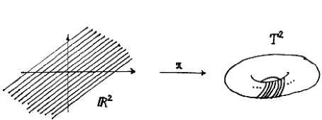
Figure 2: The linear foliations of $T^{2}$ model the noncommutative geometry of the leaf space of $\mathcal{F}$ in the case $\rho(\mathfrak{f})\leq 2$.

4.4 A “flux” criterion for the topology of $\mathcal{F}$

The criterion given above for deciding when the foliation is a fibration is expressed directly in terms of a component of the 4-form flux of eleven-dimensional supergravity, which takes the form (see (3)):

$$\mathbf{G}=\nu_{3}\wedge\mathbf{f}+\mathbf{F}~{}~{}.$$ (95)

The Bianchi identity for $\mathbf{G}$ amounts to $\mathrm{d}\mathbf{f}=0$ (which we already know to be a consequence of the supersymmetry conditions) plus the supplementary condition $\mathrm{d}\mathbf{F}=0$. Thus:

Proposition.

If there exists a positive scaling factor $\lambda\in\mathbb{R}^{\ast}_{+}$ such that $\lambda\mathfrak{f}\in H^{1}(M,\mathbb{Z})$, then all leaves of $\mathcal{F}$ are compact and $\mathcal{F}$ is a fibration over $S^{1}$, while $M$ is diffeomorphic with a mapping torus. If such a scaling factor does not exist, then the foliation $\mathcal{F}$ is minimal, i.e. each leaf of $\mathcal{F}$ is dense in $M$ and $\mathcal{F}$ cannot be a fibration (since $M$ is compact).

Remarks.

1. When passing to M theory, quantum consistency requires Witten the flux of $\mathbf{G}$ to satisfy the condition:

   $$\int_{D}\frac{\mathbf{G}}{2\pi}-\frac{1}{4}\int_{D}p_{1}(\mathbf{M})\in\mathbb{Z}~{}~{},~{}~{}\forall D\in H_{4}(\mathbf{M},\mathbb{Z})~{}~{},$$ (96)

   where $H_{\ast}(\mathbf{M},\mathbb{Z})$ denotes singular homology while $\int_{D}p_{1}(\mathbf{M})\in 2\mathbb{Z}$ since $\mathbf{M}$ is spin. One might naively imagine that this condition could constrain $\mathfrak{f}$ to be projectively rational, thus ruling out foliations $\mathcal{F}$ whose leaves are dense in $M$. This is in fact not the case, for the following reason. Since the ordinary de Rham cohomology groups of the contractible manifold $N\simeq\mathbb{R}^{3}$ are given by:

   $$H^{0}(N,\mathbb{R})\simeq\mathbb{R}~{}~{},~{}~{}H^{1}(N,\mathbb{R})=H^{2}(N,\mathbb{R})=H^{3}(N,\mathbb{R})=0~{}~{},$$

   the Kunneth theorem for de Rham cohomology gives $H^{4}(\mathbf{M},\mathbb{R})\simeq H^{0}(N,\mathbb{R})\otimes_{\mathbb{R}}H^{4}(M,\mathbb{R})\simeq H^{4}(M,\mathbb{R})$ and hence $[\frac{\mathbf{G}}{2\pi}]\equiv[\frac{\mathbf{F}}{2\pi}]$ in de Rham cohomology since $[\nu_{3}\wedge\mathbf{f}]=0$ (because the de Rham cohomology class of $[\nu_{3}]\in H^{3}(N,\mathbb{R})$ vanishes). On the other hand, we have $2p_{1}(\mathbf{M})=2\Pi_{2}^{\ast}(p_{1}(M))$ since $T{\mathbf{M}}\simeq\Pi_{1}^{\ast}(TN)\oplus\Pi_{2}^{\ast}(TM)$ (where $\Pi_{i}$ are the canonical projections of the product $N\times M$) and $TN$ is trivial. By the Kunneth theorem for singular homology, we also have:

   $$H_{4}(\mathbf{M},\mathbb{Z})\simeq H_{0}(N,\mathbb{Z})\otimes_{\mathbb{Z}}H_{4}(M,\mathbb{Z})\oplus H_{3}(N,\mathbb{Z})\otimes_{\mathbb{Z}}H_{1}(M,\mathbb{Z})\simeq H_{4}(M,\mathbb{Z})$$

   since $H_{0}(N,\mathbb{Z})\simeq\mathbb{Z}$ while $H_{1}(N,\mathbb{Z})=H_{2}(N,\mathbb{Z})=H_{3}(N,\mathbb{Z})=0$ and $\mathrm{Tor}_{1}^{\mathbb{Z}}(\mathbb{Z},H_{3}(M,\mathbb{Z}))=0$. Hence (96) is equivalent with:

   $$\int_{D}\left[\frac{\mathbf{F}}{2\pi}-\frac{1}{4}p_{1}(M)\right]\in\mathbb{Z},~{}~{}\forall D\in H_{4}(M,\mathbb{Z})~{}~{},$$

   a relation which does not involve $\mathfrak{f}$. Thus (96) does not constrain the cohomology class $\mathfrak{f}$ and hence one can expect that foliations whose leaves are dense in $M$ provide consistent backgrounds in M theory. One would of course need to perform a careful analysis of all known quantum corrections Meff around such backgrounds in order to verify this expectation, but such analysis is outside the scope of the present paper.

2. Recall that $\mathcal{F}$ is a fibration over the circle iff. $\mathfrak{f}$ is projectively rational, in which case $M$ is the mapping torus of the diffeomorphism $\phi_{a}$ of some arbitrarily chosen leaf $L$. In this case, one can view our M-theory background as a two step compactification, where in the first step one compactifies on $L$ down to four dimensions while in the second step one further compactifies the resulting four-dimensional theory by “fibering” it over the circle. When using this perspective, the diffeomorphism $\phi_{a}$ induces a symmetry of the corresponding supergravity action in four dimensions. Then the second step can be described as compactifying this four-dimensional theory over the circle using the “duality twist” provided by that symmetry. This point of view was used, for example, in reference Vandoren to describe compactifications of $M$-theory on certain seven-manifolds which are fibrations over the circle (with six-manifold fibers), where such compactifications were called “Scherk-Schwarz compactifications with a duality twist”. In our situation, the case when $\mathfrak{f}$ is projectively rational could be described in the same manner, except that one has to start with the four-dimensional supergravity theory obtained by reducing M-theory over the seven-manifold $L$ (which carries a non-parallel $G_{2}$ structure), while taking the effect of $F$ and $f$ into account (in particular, the relevant actions in both three and four dimensions will be gauged supergravity actions). When $b_{1}(M)\geq 2$, such generalized Scherk-Schwarz reductions can describe only a negligible subset of all $\mathcal{N}=1$ compactifications of $M$-theory down to $\mathrm{AdS}_{3}$, since in that case the projectively rational classes correspond to a countable subset of the projectivization $\mathbb{P}H^{1}(M,\mathbb{R})\simeq\mathbb{P}^{b_{1}(M)-1}$ of $H^{1}(M,\mathbb{R})$, which is an uncountable set. The generic compactification in our class corresponds to a minimal foliation $\mathcal{F}$ — thus being very different in nature from compactifications of generalized Scherk-Schwarz type.

5 Comparison with previous work

Relation with MartelliSparks .

The class of compactifications analyzed in this paper was pioneered in MartelliSparks , where the solution of the Fierz identities as well as certain combinations of the exterior differential and codifferential constraints analyzed in our paper were first given. Appendix C of loc. cit also lists, in a different form, a set of ‘useful relations’ which turn out, after some work ga1 , to be equivalent with what we call the $\check{Q}$-constraints. Here are some points of difference with MartelliSparks regarding the techniques that allowed us to extract the full solution. They concern the local analysis of such geometries (since the topology of the foliation $\mathcal{F}$ was not previously discussed in the literature).

• We made systematic use of the non-redundant parameterization (31), which eliminates those rank components of $\check{E}$ that are determined by the Fierz relations.

• We solved the $\check{Q}$-constraints (35) explicitly. We found that they determine certain components of $F$ as algebraic combinations of $\Delta,b,V$ and $f$, while imposing no further conditions.

• We fully encoded the supersymmetry conditions (4) through the extrinsic geometry of the foliation $\mathcal{F}$, through the non-adapted part of the normal connection $D_{n}$ and through the torsion classes of its longitudinal $G_{2}$ structure, all of which we extracted explicitly.

• We used directly the covariant derivative constraint (34) rather than the exterior differential and codifferential constraints (38) and (39) which it implies. This allowed us to give the full set of conditions characterizing supersymmetric solutions and to prove rigorously that they do so. In particular, we determined the covariant derivative of $V$, which is completely specified by the supersymmetry conditions when $\mathbf{G}$ is given.

• Details of the comparison of our results with certain relations given in MartelliSparks can be found in Appendix D.

Relation with Tsimpis .

The class of backgrounds discussed in this paper can also be approached using the method proposed in Tsimpis , which relies on the fact that existence of an everywhere non-vanishing Majorana spinor on $M$ implies that both $M$ and its orientation opposite ${\bar{M}}$ admit $\mathrm{Spin}(7)$ structures — an approach which uses explicitly only part of the full symmetry of the problem. The relation between the description presented here and that of Tsimpis is given in g2s , in the general context when $\xi$ is not required to be everywhere non-chiral. As it turns out, that case can be described using the theory of singular foliations.

6 Conclusions and further directions

We analyzed $\mathcal{N}=1$ compactifications of eleven-dimensional supergravity down to $\mathrm{AdS}_{3}$ using the theory of foliations. We found that, in the nowhere chiral case, the compactification manifold can be described through a codimension one foliation carrying a leafwise $G_{2}$ structure and that the supersymmetry conditions are equivalent with explicit equations determining the extrinsic geometry of this foliation and the torsion classes of the $G_{2}$ structure. In particular, we found that the leafwise $G_{2}$ structure is integrable (in fact, conformally co-calibrated), belonging to the Fernandez-Gray class $W_{1}\oplus W_{3}\oplus W_{4}$. We also discussed the topology of such foliations, including the non-commutative topology of their leaf space, giving a criterion which distinguishes the cases when the leaves are compact and dense, respectively. We also showed that existence of solutions requires vanishing of the Latour obstruction for the cohomology class of a certain component of the supergravity 4-form field strength. The case when $\xi$ is not everywhere non-chiral is discussed in g2s using the theory of singular foliations.

Foliations also feature in the proposals of Grana where, however, the conditions imposed by supersymmetry were not considered. It would be interesting to explore further the connection of the backgrounds discussed in this paper with the abstract classes of foliations which were discussed in loc. cit. starting from the framework of extended generalized geometry. The supersymmetric foliated backgrounds discussed in our paper could serve to realize explicitly part of the picture proposed in that reference. It is also likely that proposals such as Bonetti may be understood better by enlarging the framework Becker1 of $\mathrm{Spin}(7)$ holonomy which was used in loc. cit. to backgrounds of the type considered in this paper.

We mention that the problem of finding explicit solutions to our equations is of the type considered in Rovenski , so it could be approached through the theory of geometric flows. We also expect that a modification of the methods of FriedrichAgricola ; Puhle1 (which would adapt them to the spinor equations (4)) may allow one to draw conclusions about the existence of solutions and the dimensionality of their moduli space.

As pointed out in MartelliSparks and recalled in Section 1, the class of backgrounds we considered are consistent at the classical level. It would be interesting to study quantum corrections, using the known subleading terms of the effective action of M-theory Meff . While the appearance of non-commutative geometry in Section 4 is of purely mathematical nature (being a general phenomenon in the theory of foliations), we suspect that it in fact has a physical interpretation through the general idea of reducing quantum theories along foliations. Non-commutativity (and even non-associativity) in closed string theories was previously observed in studies of topological TopTDuality and classical TDuality T-duality and it would therefore not be surprising should its IIA incarnation turn out to have an M-theoretic origin. It would indeed appear that this is a much more general phenomenon having to do with certain limits of field theories.

Appendix A Some Kähler-Atiyah algebra relations

We summarize a few useful relations from ga1 . Given two pure rank forms $\omega\in\Omega^{\tilde{\omega}}(M)$ and $\eta\in\Omega^{\tilde{\eta}}(M)$ on an oriented $d$-dimensional Riemannian manifold $M$, one defines their geometric product through:

$$\omega\eta\stackrel{{\scriptstyle{\rm def.}}}{{=}}\sum_{m=0}^{d}(-1)^{\left[\frac{m+1}{2}\right]+m{\tilde{\omega}}}\omega\bigtriangleup_{m}\eta~{}~{},$$

where $\bigtriangleup_{m}$ denotes the generalized product of order $m$, with  ${\rm rk}(\omega\bigtriangleup_{m}\eta)={\tilde{\omega}}+{\tilde{\eta}}-2m$ .

The reversion $\tau$ of the Kähler-Atiyah algebra of $(M,g)$ is the anti-automorphism defined through $\tau(\omega)=(-1)^{\frac{\tilde{\omega}(\tilde{\omega}-1)}{2}}\omega$, while the signature $\pi$ is the automorphism defined through $\pi=\oplus_{k}{(-1)^{k}\mathrm{id}_{\Omega^{k}(M)}}$.

The Hodge operator and codifferential for pseudo-Riemannian manifolds.

For a (not necessarily compact) pseudo-Riemannian manifold $(M,g)$ of dimension $d$ and whose metric has exactly $q$ negative eigenvalues, the Hodge operator is defined through ga1 :

$$\ast\omega\stackrel{{\scriptstyle{\rm def.}}}{{=}}\tau(\omega)\nu~{}~{},$$

and we have

$$\ast^{2}=(-1)^{q}\pi^{d-1}~{}~{},~{}~{}\nu^{2}=(-1)^{q+\left[\frac{d}{2}\right]}~{}~{}$$

as well as:

$$\omega\wedge\ast\eta=\langle\omega,\eta\rangle\nu~{}~{},~{}~{}\forall\omega,\eta\in\Omega(M)~{}~{}\mathrm{with}~{}~{}{\rm rk}\omega={\rm rk}\eta~{}~{}.$$

The codifferential is defined through:

$$\updelta\omega=(-1)^{d({\tilde{\omega}}+1)+q+1}\ast\mathrm{d}\ast\omega=-\iota_{e^{a}}\nabla_{e^{a}}\omega~{}~{},~{}~{}\forall~{}\omega\in\Omega(M)~{}~{}\mathrm{with}~{}~{}{\rm rk}\omega={\tilde{\omega}}~{}~{}$$

and is the formal adjoint of $\mathrm{d}$ with respect to the non-degenerate bilinear pairing $\int_{M}\langle~{},~{}\rangle\nu$ on the subspace $\Omega_{c}(M)\subset\Omega(M)$ of compactly-supported differential forms:

$$\int_{M}\langle\mathrm{d}\omega,\eta\rangle\nu=\int_{M}\langle\omega,\updelta\eta\rangle\nu~{}~{}\forall\omega,\eta\in\Omega_{c}(M)~{}~{}.$$

Under a conformal transformation $g\rightarrow g^{\prime}\stackrel{{\scriptstyle{\rm def.}}}{{=}}e^{2\alpha}g$, the Hodge operator changes as $\ast\rightarrow\ast^{\prime}$, where:

$$\ast^{\prime}(\omega)=e^{(d-2~{}\!{\rm rk}\omega)\alpha}\ast\omega~{}~{},~{}~{}\mathrm{for}~{}\omega~{}\mathrm{of~{}pure~{}rank.}$$

Identities for Riemannian manifolds.

For the rest of this Appendix, we assume that $M$ is Riemannian. If $\nu$ is the volume form of $(M,g)$, while $\ast$ is the Hodge operator, then the following identities hold:

$$\ast\omega = \iota_{\omega}\nu=\tau(\omega)\nu~{},$$

$$\nu\omega = \pi^{d-1}(\omega)\nu~{},$$

$$\ast^{2}=\pi^{d-1}~{} ~{}~{}~{}\nu^{2}=(-1)^{[\frac{d}{2}]}~{},$$ , (97)

$$\omega\bigtriangleup_{\tilde{\omega}}\eta = \iota_{\tau(\omega)}\eta=\eta\bigtriangleup_{\tilde{\omega}}\omega~{},$$

$$\omega\wedge\ast\eta=(-1)^{\tilde{\omega}(\tilde{\eta}-1)}\ast(\iota_{\tau(\omega)}\eta)~{},~{}~{}{\rm when}~{}~{}\tilde{\omega}\leq\tilde{\eta}~{},$$

$$\iota_{\omega}(\ast\eta)=(-1)^{\tilde{\omega}\tilde{\eta}}\ast(\tau(\omega)\wedge\eta)~{},~{}~{}{\rm when}~{}~{}\tilde{\omega}+\tilde{\eta}\leq d~{},$$ (98)

$$(-1)^{[\frac{m+1}{2}]}\pi^{m}(\omega)\bigtriangleup_{m}[\ast\tau(\eta)] = (-1)^{[\frac{m^{\prime}+1}{2}]}[\ast\tau(\omega)]\bigtriangleup_{m^{\prime}}\pi^{d-1}(\eta)$$ (99)

$$= (-1)^{[\frac{m^{\prime\prime}+1}{2}]}\ast\tau\left[\pi^{m^{\prime\prime}}(\omega)\bigtriangleup_{m^{\prime\prime}}\eta\right]~{},$$

$$\mathrm{for}~{}~{}~{}\tilde{\omega}-m = \tilde{\eta}-m^{\prime}=m^{\prime\prime}~{},~{}~{}\mathrm{where}~{}~{}m,m^{\prime},m^{\prime\prime}>0~{}~{}.$$

Any pure rank form decomposes uniquely into parallel and orthogonal components w.r.t any 1-form $u$ of unit norm $||u||=1$  ,

$$\omega=\omega_{\perp}+\omega_{\parallel}=\omega_{\perp}+u\wedge\omega_{\top}~{}~{},$$

where $\omega_{\top}\stackrel{{\scriptstyle{\rm def.}}}{{=}}\iota_{u}\omega$ and $\omega_{\perp}\stackrel{{\scriptstyle{\rm def.}}}{{=}}\omega-u\wedge\iota_{u}\omega$ are the top and orthogonal parts of $\omega$ discussed in ga1 . If $\ast_{\perp}\eta\stackrel{{\scriptstyle{\rm def.}}}{{=}}\ast(u\wedge\eta)$ denotes the Hodge operator along the Frobenius distribution $\mathcal{D}$ transverse to $u$ (the Hodge operator defined on $\mathcal{D}$ by the induced metric, when $\mathcal{D}$ is endowed with the orientation given by the volume form $\nu_{\top}=\iota_{u}\nu$ along $\mathcal{D}$), then one has the identities, which can be used to decompose various formulas into components along $\mathcal{D}$ and $\mathcal{D}^{\perp}$:

$$(u\wedge\omega)_{\perp}=0~{}~{}~{} ~{}~{}~{}(u\wedge\omega)_{\top}=\omega_{\perp}~{},$$ ,

$$(\iota_{u}\omega)_{\perp}=\omega_{\top}~{}~{}~{} ~{}~{}~{}(\iota_{u}\omega)_{\top}=0~{},$$ ,

$$\ast\omega=\ast_{\perp}(\omega_{\top}) + u\wedge\ast_{\perp}\pi(\omega_{\perp})~{},$$

$$(\ast\omega)_{\perp}=\ast_{\perp}(\omega_{\top})~{}~{}~{} ~{}~{}~{}(\ast\omega)_{\top}=\ast_{\perp}\pi(\omega_{\perp})~{},$$ ,

$$\tau(\omega)_{\perp}=\tau(\omega_{\perp})~{}~{}~{} ~{}~{}~{}\tau(\omega)_{\top}=\pi(\tau(\omega_{\top}))~{}~{}$$ ,

$$\pi(\omega)_{\perp}=\pi(\omega_{\perp})~{}~{}~{} ~{}~{}~{}\pi(\omega)_{\top}=-\pi(\omega_{\top})~{}~{}$$ ,

$$(\omega\eta)_{\perp}=\omega_{\perp}\eta_{\perp}+\pi(\omega_{\top})\eta_{\top}~{}~{} ~{}~{}(\omega\eta)_{\top}=\omega_{\top}\eta_{\perp}+\pi(\omega_{\perp})\eta_{\top}~{}~{}$$ ,

$$(\nu\omega)_{\perp}=-\nu_{\top}\omega_{\top}~{}~{} ~{}~{}(\nu\omega)_{\top}=\nu_{\top}\omega_{\perp}$$ ,

$$(\omega\nu)_{\perp}=\pi(\omega_{\top})\nu_{\top}~{}~{} ~{}~{}(\omega\nu)_{\top}=\pi(\omega_{\perp})\nu_{\top}~{}~{}.$$ ,

For $\alpha\in\Omega^{1}(M)$ such that $\alpha\perp u$, we have:

$$(\alpha\wedge\omega)_{\perp}=\alpha\wedge(\omega_{\perp})~{}~{} ~{}~{}(\alpha\wedge\omega)_{\top}=-\alpha\wedge(\omega_{\top})~{}~{},$$ ,

$$(\iota_{\alpha}\omega)_{\perp}=\iota_{\alpha}(\omega_{\perp})~{}~{} ~{}~{}(\iota_{\alpha}\omega)_{\top}=-\iota_{\alpha}(\omega_{\top})~{}~{}.$$ ,

When $\dim M=8$, the canonical trace of the Kähler-Atiyah algebra is given by ga1 :

$$\mathcal{S}(\omega)=16\omega^{(0)}~{}~{},~{}~{}$$

where $\omega^{(0)}$ denotes the rank zero component of the inhomogeneous form $\omega\in\Omega(M)$. Furthermore:

$$\ast^{2}=\pi~{}~{},~{}~{}\nu^{2}=+1~{}~{}$$

and $\nu$ is twisted central (i.e. $\omega\nu=\nu\pi(\omega)$) in the Kähler-Atiyah algebra of $M$. We also mention the following relation which holds when $(M,g)$ is an eight-dimensional Riemannian manifold.

$$\mathcal{S}(\omega^{2})=16(-1)^{\left[\frac{k}{2}\right]}||\omega||^{2}~{}~{},~{}~{}\forall\omega\in\Omega^{k}(M)~{}~{}.$$ (100)

Appendix B Useful identities for manifolds with $G_{2}$ structure

On the 7-dimensional leaves of the foliation $\mathcal{F}$ we have a $G_{2}$ structure. Our computations rely on various identities for such structures (see, for example, Kthesis ; Kflows ) and on the decomposition of the exterior bundle of the leaves into vector sub-bundles carrying fiberwise irreps. of $G_{2}$ FG ; BryantEH ; Bryant . Notice that all statements of this Appendix generalize trivially to $G_{2}$ structures defined on (necessarily orientable) vector bundles of rank seven, such as the Frobenius distribution $\mathcal{D}$ of this paper.

Let $L$ be a 7-manifold endowed with a a $G_{2}$ structure described by the canonically normalized associative 3-form $\varphi$. Since $G_{2}$ is a subgroup of $\mathrm{SO}(7)$, $\varphi$ determines both a metric $g\stackrel{{\scriptstyle{\rm def.}}}{{=}}g_{\varphi}$ and an orientation of $L$, the metric being fixed uniquely by the following condition, where $\nu_{L}$ is the corresponding volume form of $L$ (see Kthesis ):

$$(v\lrcorner\varphi)\wedge(w\lrcorner\varphi)\wedge\varphi=-6g(v,w)\nu_{L}~{}~{},~{}~{}v,w\in\Gamma(L,TL)~{}~{}.$$

The $G_{2}$ structure is also determined by the coassociative 4-form $\psi=\ast_{L}\varphi$, where $\ast_{L}\stackrel{{\scriptstyle{\rm def.}}}{{=}}\ast_{\varphi}$ is the Hodge operator defined by $g_{\varphi}$ and by the orientation induced by $\varphi$. The canonical normalization conditions are:

$$||\varphi||^{2}=||\psi||^{2}=7~{}~{}.$$

The bundles of 1- and 6-forms (which are Hodge dual to each other) carry irreducible fiberwise representations, while the bundles of 2, 3, 4 and 5-forms decompose canonically into vector bundles carrying fiberwise irreps. This leads to the following decompositions of the ${{\cal\mathcal{C}}^{\infty}(M,\mathbb{R})}$-modules of pure rank forms FG ; BryantEH ; Bryant ; Kflows :

$$\Omega^{2}(L) = \Omega^{2}_{7}(L)\oplus\Omega^{2}_{14}(L)~{}~{},~{}~{}\Omega^{3}(L)=\Omega^{3}_{1}(L)\oplus\Omega^{3}_{7}(L)\oplus\Omega^{3}_{27}(L)~{}~{},$$

$$\Omega^{5}(L) = \Omega^{5}_{7}(L)\oplus\Omega^{5}_{14}(L)~{}~{},~{}~{}\Omega^{4}(L)=\Omega^{4}_{1}(L)\oplus\Omega^{4}_{7}(L)\oplus\Omega^{4}_{27}(L)~{}~{},$$

where the subscript indicates the dimension of the corresponding irrep. of $G_{2}$. For convenience, we set $\Omega^{k}_{S}(L)\stackrel{{\scriptstyle{\rm def.}}}{{=}}\Omega^{k}_{1}(L)\oplus\Omega^{k}_{27}(L)$ for $k=3,4$. The Hodge operator $\ast_{L}$ maps $\Omega^{2}(L)$ into $\Omega^{5}(L)$ and $\Omega^{3}(L)$ into $\Omega^{4}(L)$ preserving these decompositions. The modules $\Omega^{3}_{7}(L)$ and $\Omega^{4}_{7}(L)$ are both isomorphic with $\Omega^{1}(L)$, while $\Omega^{3}_{S}(L)$ is isomorphic with the ${{\cal\mathcal{C}}^{\infty}(M,\mathbb{R})}$-module of symmetric 2-tensors, with $\Omega^{k}_{27}(L)$ corresponding to traceless symmetric tensors. More precisely, any four-form $\omega\in\Omega^{4}(L)$ decomposes as:

$$\omega=\omega^{(7)}+\omega^{(S)}~{}~{},~{}~{}{\rm with}~{}~{}\omega^{(7)}\in\Omega^{4}_{7}(L)~{},~{}\omega^{(S)}\in\Omega^{4}_{S}(L)~{}~{},$$

while the components can be parameterized as follows BryantEH ; Bryant ; Kflows :

$$\omega^{(7)}=\alpha\wedge\varphi~{},~{}~{}\alpha\in\Omega^{1}(L)~{}~{},~{}~{}\omega^{(S)}=-\hat{h}_{ij}e^{i}\wedge\iota_{e^{j}}\psi~{},$$ (101)

where $\hat{h}_{ij}$ is a symmetric tensor. The decomposition ${\hat{h}}_{ij}=\frac{1}{7}\mathrm{tr}_{g}({\hat{h}})g_{ij}+{\hat{h}}_{ij}^{(0)}$ with $\mathrm{tr}_{g}({\hat{h}}^{(0)})=0$ gives $\omega^{(S)}=\omega^{(1)}+\omega^{(27)}$, where $\omega_{1}=-\frac{4}{7}\mathrm{tr}_{g}({\hat{h}})\psi\in\Omega^{4}_{1}(L)$ and $\omega^{(27)}=-\hat{h}^{(0)}_{ij}e^{i}\wedge\iota_{e^{j}}\psi\in\Omega^{4}_{27}(L)$.

Similarly, any 3-form $\eta\in\Omega^{3}(L)$ decomposes as:

$$\eta~{}=\eta^{(7)}+\eta^{(S)}~{}~{},~{}~{}{\rm with}~{}~{}\eta^{(7)}\in\Omega^{3}_{7}(L)~{},~{}\eta^{(S)}\in\Omega^{3}_{S}(L)~{},$$

where the components can be parameterized through BryantEH ; Bryant ; Kflows :

$$\eta^{(7)}=-\iota_{\alpha}\psi~{},~{}~{}\alpha\in\Omega^{1}(L)~{}~{},~{}~{}\eta^{(S)}=h_{ij}e^{i}\wedge\iota_{e^{j}}\varphi~{},$$ (102)

with $h_{ij}$ a symmetric tensor. The decomposition $h_{ij}=\frac{1}{7}\mathrm{tr}_{g}(h)g_{ij}+h_{ij}^{(0)}$ with $\mathrm{tr}_{g}(h^{(0)})=0$ gives $\eta^{(S)}=\eta^{(1)}+\eta^{(27)}$ with $\eta_{1}=\frac{3}{7}\mathrm{tr}_{g}(h)\varphi\in\Omega^{3}_{1}(L)$ and $\eta^{(27)}=h^{(0)}_{ij}e^{i}\wedge\iota_{e^{j}}\varphi\in\Omega^{3}_{27}(L)$.

Given $\eta^{(S)}\in\Omega^{3}(L)$, the corresponding symmetric tensor $h$ which satisfies the second equation of (102) is uniquely determined and given by the formula FG ; BryantEH ; Bryant ; Kflows :

$$h_{ij}=-\frac{1}{2}\mathrm{tr}_{g}(h)g_{ij}-\frac{1}{4}\ast_{L}(\iota_{e^{i}}\varphi\wedge\iota_{e^{j}}\varphi\wedge\eta^{(S)})=-\frac{1}{2}\mathrm{tr}_{g}(h)g_{ij}-\frac{1}{4}\left[\langle\iota_{e^{i}}\varphi,\iota_{e^{j}}\eta^{(S)}\rangle+(i\leftrightarrow j)\right]~{}~{}.$$ (103)

Furthermore, $\omega^{(S)}$ and $\eta^{(S)}$ are Hodge dual to each other iff. $h$ and ${\hat{h}}$ are related through:

$${\hat{h}}_{ij}=h_{ij}-\frac{1}{4}\mathrm{tr}_{g}(h)g_{ij}\Longleftrightarrow h_{ij}=\hat{h}_{ij}-\frac{1}{3}\mathrm{tr}_{g}(\hat{h})g_{ij}~{}~{},$$

a relation which implies $\mathrm{tr}_{g}({\hat{h}})=-\frac{3}{4}\mathrm{tr}_{g}(h)\Longleftrightarrow\mathrm{tr}_{g}(h)=-\frac{4}{3}~{}\mathrm{tr}_{g}(\hat{h})$. This amounts to the requirement that $\omega^{(1)}$ and $\eta^{(1)}$ are Hodge dual to each other and that the same holds for $\omega^{(27)}$ and $\eta^{(27)}$. One also notices $\hat{h}^{(0)}=h^{(0)}$.

The torsion classes $\boldsymbol{\tau}_{0}\in\Omega^{0}_{1}(L)$, $\boldsymbol{\tau}_{1}\in\Omega^{1}_{7}(L)$, $\boldsymbol{\tau}_{2}\in\Omega^{2}_{14}(L)$ and $\boldsymbol{\tau}_{3}\in\Omega^{3}_{27}(L)$ of the $G_{2}$ structure are uniquely specified through the following equations, which follow the conventions of Bryant ; Kflows :

$$\begin{split}&\mathrm{d}_{\perp}\varphi=\boldsymbol{\tau}_{0}\psi+3\boldsymbol{\tau}_{1}\wedge\varphi+\ast_{\perp}\boldsymbol{\tau}_{3}~{}~{},\\ &\mathrm{d}_{\perp}\psi=4\boldsymbol{\tau}_{1}\wedge\psi+\ast_{\perp}\boldsymbol{\tau}_{2}~{}~{}.\\ \end{split}$$ (104)

Since the torsion class $\boldsymbol{\tau_{3}}$ belongs to $\Omega^{3}_{27}(L)$, it can be parameterized through a traceless symmetric tensor $t_{ij}$: :

$$\boldsymbol{\tau}_{3}=t_{ij}e^{i}\wedge\iota_{e^{j}}\varphi~{}~{},$$ (105)

where $t_{ij}$ can be recovered from $\boldsymbol{\tau}_{3}$ through relation (103):

$$t_{ij}=-\frac{1}{4}\left[\langle\iota_{e_{i}}\varphi,\iota_{e_{j}}\tau_{3}\rangle+(i\leftrightarrow j)\right]~{}~{}.$$ (106)

Under a conformal transformation with conformal factor $e^{2\alpha}$, we have:

$$\begin{split}&g^{\prime}_{ij}=e^{2\alpha}g_{ij}~{}~{},~{}~{}\nu_{L}^{\prime}=e^{7\alpha}\nu_{L}~{}~{}~{}~{}~{}~{}~{}~{}~{}~{},~{}~{}\varphi^{\prime}=e^{3\alpha}\varphi~{}~{}~{},~{}~{}\psi^{\prime}=e^{4\alpha}\psi~{},\\ &\boldsymbol{\tau}^{\prime}_{0}=e^{\alpha}\boldsymbol{\tau}_{0}~{}~{}~{},~{}~{}\boldsymbol{\tau}^{\prime}_{1}=e^{\alpha}(\boldsymbol{\tau}_{1}+\mathrm{d}\alpha)~{}~{},~{}~{}\boldsymbol{\tau}^{\prime}_{2}=e^{\alpha}\boldsymbol{\tau}_{2}~{}~{},~{}~{}\boldsymbol{\tau}^{\prime}_{3}=e^{\alpha}\boldsymbol{\tau}_{3}~{}~{}\end{split}$$ (107)

and $\ast^{\prime}_{L}\omega=e^{(7-2{\rm rk}\omega)\alpha}\ast_{L}\omega$ for any pure rank form $\omega\in\Omega(L)$.

For reader’s convenience, we reproduce the following identities given in Kflows , where indices are raised and lowered using the metric $g=g_{\varphi}$ and implicit summation over repeated indices is understood:

• Contractions between $\varphi$ and $\varphi$

  $$\varphi_{ijk}\varphi^{ijk} = 42~{},$$

  $$\varphi_{ijk}\varphi_{a}{}^{jk} = 6g_{ia}~{},$$ (108)

  $$\varphi_{ijk}\varphi_{ab}{}^{k} = g_{ia}g_{jb}-g_{ib}g_{ja}-\psi_{ijab}~{},$$

• Contractions between $\varphi$ and $\psi$

  $$\varphi_{ijk}\psi_{a}{}^{ijk} = 0~{},$$

  $$\varphi_{ijk}\psi_{ab}{}^{jk} = -4\varphi_{iab}~{},$$ (109)

  $$\varphi_{ijk}\psi_{abc}{}^{k} = g_{ia}\varphi_{jbc}+g_{ib}\varphi_{ajc}+g_{ic}\varphi_{abj}-g_{aj}\varphi_{ibc}-g_{bj}\varphi_{aic}-g_{cj}\varphi_{abi}~{},$$

• Contractions between $\psi$ and $\psi$

  $$\psi_{ijkl}\psi^{ijkl} = 168~{},$$

  $$\psi_{ijkl}\psi_{a}{}^{jkl} = 24g_{ia}~{},$$

  $$\psi_{ijkl}\psi_{ab}{}^{kl} = 4g_{ia}g_{jb}-4g_{ib}g_{ja}-2\psi_{ijab}~{},$$

  $$\psi_{ijkl}\psi_{abc}{}^{l} = -\varphi_{ajk}\varphi_{ibc}-\varphi_{iak}\varphi_{jbc}-\varphi_{ija}\varphi_{kbc}$$

  $$+g_{ia}g_{jb}g_{kc}+g_{ib}g_{jc}g_{ka}+g_{ic}g_{ja}g_{kb}$$

  $$-g_{ia}g_{jc}g_{kb}-g_{ib}g_{ja}g_{kc}-g_{ic}g_{jb}g_{ka}$$

  $$-g_{ia}\psi_{jkbc}-g_{ja}\psi_{kibc}-g_{ka}\psi_{ijbc}$$

  $$+g_{ab}\psi_{ijkc}-g_{ac}\psi_{ijkb}~{}.$$

• For any 1-form $\alpha$ and any vector field $w$, the following identities hold Kthesis :

  $$\varphi\wedge\ast_{L}(\alpha\wedge\varphi)=4\ast_{L}\alpha~{}~{}~{}~{} ~{}~{}~{}~{}\varphi\wedge(w~{}\lrcorner~{}\psi)=-4\ast_{L}w^{\#}~{},$$ ,

  $$\psi\wedge\ast_{L}(\alpha\wedge\psi)=3\ast_{L}\alpha~{}~{}~{}~{} ~{}~{}~{}~{}\psi\wedge(w~{}\lrcorner\varphi)=3\ast_{L}w^{\#}~{},$$ ,

  $$\psi\wedge\ast_{L}(\alpha\wedge\varphi)=0~{}~{}~{}~{} ~{}~{}~{}~{}\psi\wedge(w~{}\lrcorner~{}\psi)=0~{},$$ , (111)

  $$\varphi\wedge\ast_{L}(\alpha\wedge\psi)=-2~{}\alpha\wedge\psi~{}~{}~{}~{} ~{}~{}~{}~{}\varphi\wedge(w~{}\lrcorner~{}\varphi)=-2\ast_{L}(w~{}\lrcorner~{}\varphi)~{}.$$ ,

Remark.

Formulas for contractions and for projectors on $G_{2}$ representations can also be found in GrigorianYau ; Grigorian .

The contractions listed above imply that the canonically-normalized coassociative form $\psi$ satisfies the following identity in the Kähler-Atiyah algebra of $L$:

$$\psi^{2}=6\psi+7~{}~{},$$ (112)

which amounts to the statement that:

$$\Pi\stackrel{{\scriptstyle{\rm def.}}}{{=}}\frac{1}{8}(1+\psi)~{}~{}$$

is an idempotent in the Kähler-Atiyah algebra.

The right action of $\psi$ on 4-forms and 3-forms in the Kähler-Atiyah algebra.

Let $\omega\in\Omega^{4}(L)$. Then:

$${\mathcal{R}}_{\psi}(\omega)\stackrel{{\scriptstyle{\rm def.}}}{{=}}\omega\psi=-\omega\bigtriangleup_{1}\psi-\omega\bigtriangleup_{2}\psi+\omega\bigtriangleup_{3}\psi+\omega\bigtriangleup_{4}\psi~{}~{}.$$

Using the $G_{2}$-structure identities and the parameterization of $\omega^{(7)}$ and $\omega^{(S)}$ given in (101), one finds:

$$\omega\psi=4\ast_{L}\alpha-4~{}\mathrm{tr}_{g}(\hat{h})\psi-\omega^{(S)}+3\omega^{(7)}+4\iota_{\alpha}\varphi-4~{}\mathrm{tr}_{g}(\hat{h})~{}~{}.$$ (113)

This implies $\ker({\cal R}_{\psi}|_{\Omega^{4}(L)})=0$. Similarly, for any $\eta\in\Omega^{3}(L)$, we have:

$${\mathcal{R}}_{\psi}(\eta)\stackrel{{\scriptstyle{\rm def.}}}{{=}}\eta\psi=\eta\wedge\psi+\eta\bigtriangleup_{1}\psi-\eta\bigtriangleup_{2}\psi-\eta\bigtriangleup_{3}\psi~{}~{}.$$

This can be computed either directly using the identities of Appendix B or by Hodge dualizing (113) (using $\eta\psi=(\ast_{L}\omega)\psi=\omega\nu\psi=(\omega\psi)\nu$ ). This gives:

$$\eta\psi=3~{}\mathrm{tr}_{g}(h)\nu-4\alpha\wedge\psi-\eta^{(S)}+3\eta^{(7)}+3~{}\mathrm{tr}_{g}(h)\varphi-4\alpha~{},$$ (114)

where $\eta$ is parameterized as in (102) and implies $\ker({\cal R}_{\psi}|_{\Omega^{3}(L)})=0$. Finally, we recall the following identities:

$$(\ast_{L})^{2}=\mathrm{id}_{\Omega(M)}~{}~{},~{}~{}(\nu_{L})^{2}=-1~{}~{}$$

and the fact that $\nu_{L}$ is central in the Kähler-Atiyah algebra of $L$ (i.e. $\lambda\nu_{L}=\nu_{L}\lambda~{},~{}\forall\lambda\in\Omega(L)$).

Appendix C Characterizing the extrinsic geometry of $\mathcal{F}$

C.1 Fundamental second order objects

The vector field $n=\hat{V}^{\sharp}$ has unit norm and is orthogonal to $\mathcal{F}$. Any $X\in\Gamma(M,TM)$ decomposes as $X=g(n,X)n+X_{\perp}$, where $X_{\perp}\perp n$. Since $g(n,n)=1$, one has $g(n,\nabla_{X}n)=\frac{1}{2}[g(\nabla_{X}n,n)+g(n,\nabla_{X}n)]=\frac{1}{2}X(g(n,n))=0$, i.e. $\nabla_{X}n$ is orthogonal to $n$. The second order data of $\mathcal{F}$ and $\mathcal{F}^{\perp}$ are encoded by the following objects:

For the foliation $\mathcal{F}$:

• $\nabla^{\perp}:\Gamma(M,\mathcal{D})\times\Gamma(M,\mathcal{D})\rightarrow\Gamma(M,\mathcal{D})$, the Levi-Civita connection of the metric induced by $g$ on the leaves of $\mathcal{F}$ (this is a partial connection on $M$, valued in $\mathcal{D}$)

• $B:\Gamma(M,\mathcal{D})\times\Gamma(M,\mathcal{D})\rightarrow{{\cal\mathcal{C}}^{\infty}(M,\mathbb{R})}$, $B(X_{\perp},Y_{\perp})\stackrel{{\scriptstyle{\rm def.}}}{{=}}g(n,\nabla_{X_{\perp}}Y_{\perp})$, the scalar second fundamental form of the foliation $\mathcal{F}$ (the full second fundamental form is given by $Bn$)

• $A:\Gamma(M,\mathcal{D})\rightarrow\Gamma(M,\mathcal{D})$, $A(X_{\perp})\stackrel{{\scriptstyle{\rm def.}}}{{=}}-(\nabla_{X_{\perp}}n)^{\perp}$, the Weingarten operator at $n$ of the leaves of $\mathcal{F}$

• $\delta:\Gamma(M,\mathcal{D})\rightarrow{{\cal\mathcal{C}}^{\infty}(M,\mathbb{R})}$, $\delta(X)=g(n,D_{X}^{\mathcal{F}}n)$, where $D^{\mathcal{F}}$ is the normal connection along the leaves of $\mathcal{F}$.

For the foliation $\mathcal{F}^{\perp}$:

• $a\in{{\cal\mathcal{C}}^{\infty}(M,\mathbb{R})}$, the unique connection coefficient (with respect to the frame given by $n$) of the Levi-Civita connection of the metric induced by $g$ on the leaves of $\mathcal{F}^{\perp}$

• $H\stackrel{{\scriptstyle{\rm def.}}}{{=}}\nabla_{n}n\in\Gamma(M,\mathcal{D})$, the value of the second fundamental form of $\mathcal{F}^{\perp}$ on the pair $(n,n)$ of vector fields tangent to $\mathcal{F}^{\perp}$

• $W:\Gamma(M,\mathcal{D})\rightarrow{{\cal\mathcal{C}}^{\infty}(M,\mathbb{R})}$, $W(X_{\perp})\stackrel{{\scriptstyle{\rm def.}}}{{=}}-g(n,\nabla_{n}X_{\perp})$, the value at $(n,n)$ of the covariant Weingarten tensor at $X$ of the leaves of $\mathcal{F}^{\perp}$

• $D_{n}:\Gamma(M,\mathcal{D})\rightarrow\Gamma(M,\mathcal{D})$, the normal covariant derivative with respect to $n$ along the leaves of $\mathcal{F}^{\perp}$.

Gauss’s theorem for $\mathcal{F}$ amounts to the identity $\nabla^{\perp}_{X_{\perp}}Y^{\perp}=(\nabla_{X_{\perp}}Y_{\perp})^{\perp}$ plus the fact that $B$ is a symmetric tensor. Weingarten’s theorem for $\mathcal{F}$ amounts to the identity $g(A(X_{\perp}),Y_{\perp})=B(X_{\perp},Y_{\perp})$ plus the statement that $D^{\mathcal{F}}$ preserves the metric induced on the normal bundle $N\mathcal{F}=\mathcal{D}^{\perp}$, which is equivalent with the statement that the map $\delta$ vanishes. It follows that $\nabla^{\perp}$ and $A$ encode all information contained in the second order data of $\mathcal{F}$. Gauss’s theorem for $\mathcal{F}^{\perp}$ amounts to the fact that $a$ vanishes; symmetry of the second fundamental form is automatic in this case since the leaves are one-dimensional. Weingarten’s theorem amounts to the identity $W(X_{\perp})=-g(H,X_{\perp})$ plus the statement that $D_{n}$ is compatible with the metric induced on $N(\mathcal{F}^{\perp})=\mathcal{D}$. Hence $H$ and $D_{n}$ encode all information contained in the second order data of $\mathcal{F}^{\perp}$. Summarizing, we can take $H$, $A$, $\nabla^{\perp}$ and $D_{n}$ to be the fundamental second order data of the foliation $\mathcal{F}$ in the presence of the metric $g$ and write its fundamental equations as in (52).

Local expressions.

Let $e_{a}$ be a (generally non-holonomic) local frame of $M$ such that $e_{1}=n$ and $e_{j}\perp n$ and let $\Omega_{ab}^{c}$ be the connection coefficients in this frame:

$$\nabla_{e_{a}}e_{b}=\Omega_{ab}^{c}e_{c}~{}~{}.$$

Expanding $H=H^{j}e_{j}$, we have $g_{11}=1$ and $g_{1j=0}$ as well as:

$$\Omega_{11}^{1}=\Omega_{i1}^{1}=0~{}~{},~{}~{}\Omega_{11}^{j}=H^{j}~{}~{},~{}~{}\Omega_{i1}^{j}=-A_{i}^{j}~{}~{},~{}~{}\Omega_{ij}^{1}=A_{ij}~{}~{},~{}~{}\nabla^{\perp}_{e_{i}}e_{j}=\Omega_{ij}^{k}e_{k}~{}~{}.$$ (115)

The last equation says that $\Omega_{ij}^{k}$ are the connection coefficients of the leafwise partial connection $\nabla^{\perp}$ in the (generally non-holonomic) frame $(e_{i})_{i=2,\ldots,8}$ of $\mathcal{D}$. The identity $\Omega_{abc}=-\Omega_{acb}$ satisfied by the quantity $\Omega_{abc}\stackrel{{\scriptstyle{\rm def.}}}{{=}}g_{bf}\Omega_{ac}^{f}$ amounts to the condition that the tensor $A_{ij}\stackrel{{\scriptstyle{\rm def.}}}{{=}}g(Ae_{i},e_{j})$ is symmetric. Notice the relations:

$$\Omega_{i1j}=-\Omega_{ij1}=A_{ij}~{}~{},~{}~{}\Omega_{1j1}=H_{j}\stackrel{{\scriptstyle{\rm def.}}}{{=}}g_{jk}H^{k}~{}~{}.$$

C.2 The Naveira tensor of $\mathcal{P}$

Recall that every orthogonal (i.e. $g$-compatible) almost product structure $\mathcal{P}$ on $(M,g)$ corresponds to a $g$-orthogonal decomposition $TM=\mathcal{D}\oplus\mathcal{D}^{\perp}$, where $\mathcal{D}$, $\mathcal{D}^{\perp}$ are the eigen-subbundles of $TM$ corresponding to the eigenvalues $+1$ and $-1$ of $\mathcal{P}$ respectively (thus $\mathcal{P}=\mathrm{id}_{\mathcal{D}}\oplus(-\mathrm{id}_{\mathcal{D}})$). Such almost product structures can be classified Naveira ; GilMedrano ; Miquel ; Montesinos using the Naveira tensor $\mathcal{N}_{\mathcal{P}}=\nabla\Phi_{\mathcal{P}}\in\Gamma(M,(T^{\ast}M)^{\otimes 3})$, which is given by:

$$\mathcal{N}_{\mathcal{P}}(X,Y,Z)=(\nabla_{X}\Phi_{\mathcal{P}})(Y,Z)=g((\nabla_{X}\mathcal{P})Y,Z)~{}~{},~{}~{}\forall X,Y,Z\in\Gamma(M,TM)~{}~{}.$$

Here, $\Phi_{\mathcal{P}}\in\Gamma(M,\mathrm{Sym}^{2}(T^{\ast}M))$ is the symmetric covariant 2-tensor given by $\Phi_{\mathcal{P}}(X,Y)\stackrel{{\scriptstyle{\rm def.}}}{{=}}g(\mathcal{P}X,Y)$, which vanishes for $(X,Y)\in\Gamma(M,\mathcal{D}\times\mathcal{D}^{\perp}\oplus\mathcal{D}^{\perp}\times\mathcal{D})$ and whose restrictions to $\mathcal{D}$ and $\mathcal{D}^{\perp}$ equal plus and minus the restrictions of $g$, respectively. The Naveira tensor is symmetric in its last two variables and satisfies $\mathcal{N}(X,\mathcal{P}Y,\mathcal{P}Z)=-\mathcal{N}(X,Y,Z)$ and thus it vanishes when both $X,Y$ belong to $\mathcal{D}$ or to $\mathcal{D}^{\perp}$. When both $\mathcal{D}$ and $\mathcal{D}^{\perp}$ are integrable, an easy computation gives:

$$(\nabla_{X}\mathcal{P})Y = 2h_{\mathcal{D}}(X,Y)~{}~{}\mathrm{for}~{}~{}X,Y\in\Gamma(M,\mathcal{D})~{}~{},$$

$$(\nabla_{X}\mathcal{P})Y = 2h_{\mathcal{D}^{\perp}}(X,Y)~{}~{}\mathrm{for}~{}~{}X,Y\in\Gamma(M,\mathcal{D}^{\perp})~{}~{},$$

where $h_{\mathcal{D}}$ and $h_{\mathcal{D}^{\perp}}$ are the second fundamental forms of $\mathcal{D}$ and $\mathcal{D}^{\perp}$. Thus:

$$\mathcal{N}_{\mathcal{P}}(X,Y,Z) = 2g(h_{\mathcal{D}}(X,Y),Z)~{}~{}\mathrm{for}~{}~{}X,Y\in\Gamma(M,\mathcal{D})~{},~{}Y\in\Gamma(M,\mathcal{D}^{\perp})~{}~{},$$

$$\mathcal{N}_{\mathcal{P}}(X,Y,Z) = 2g(h_{\mathcal{D}^{\perp}}(X,Y),Z)~{}~{}\mathrm{for}~{}~{}X,Y\in\Gamma(M,\mathcal{D}^{\perp})~{}~{},~{}~{}Y\in\Gamma(M,\mathcal{D})~{}~{}.$$ (116)

For our distributions $\mathcal{D}=T\mathcal{F}$ and $\mathcal{D}^{\perp}=T(\mathcal{F}^{\perp})$, we find:

$$h_{\mathcal{D}}(X_{\perp},Y_{\perp}) = B(X_{\perp},Y_{\perp})n=g(AX_{\perp},Y_{\perp})n~{}~{},$$

$$h_{\mathcal{D}^{\perp}}(n,n)~{}~{} = H~{}~{},$$

so (C.2) give the following relations, which completely specify the Naveira tensor of $\mathcal{P}$:

$$\begin{split}&\mathcal{N}_{\mathcal{P}}(X_{\perp},Y_{\perp},n)=B(X_{\perp},Y_{\perp})=g(AX_{\perp},Y_{\perp})~{}~{},\\ &\mathcal{N}_{\mathcal{P}}(n,n,X_{\perp})~{}~{}~{}=2g(H,X_{\perp})~{}~{}.\end{split}~{}~{}$$

Notice that $\mathcal{N}_{\mathcal{P}}$ contains the same information as $H$ and $A$ and hence determining the latter amounts to determining $\mathcal{N}_{\mathcal{P}}$.

When $\mathcal{D}$ is integrable, with $\mathcal{D}=T\mathcal{F}$, one has the following formulas for the components of the covariant derivative, differential and codifferential of arbitrary forms $\omega\in\Omega(M)$.

The covariant derivative of forms longitudinal to $\mathcal{F}$.

Direct computation using (52) gives:

$$(\nabla_{n}\omega)_{\top}=\iota_{\hat{V}}~{}\nabla_{n}\omega=n\lrcorner\nabla_{n}\omega=-H\lrcorner\omega~{}~{} ~{}~{}(\nabla_{{}_{X_{\perp}}}\omega)_{\top}=n\lrcorner(\nabla_{{}_{X_{\perp}}}\omega)=(AX_{\perp})\lrcorner\omega~{}~{},$$ ,

$$(\nabla_{n}\omega)_{\perp}=D_{n}\omega~{}~{}~{}~{}~{}~{}~{}~{}~{}~{}~{}~{}~{}~{}~{}~{}~{}~{}~{}~{}~{}~{}~{}~{}~{}~{}~{}~{}~{}~{}~{}~{} ~{}~{}(\nabla_{X_{\perp}}\omega)_{\perp}=\nabla^{\perp}_{{}_{X_{\perp}}}\omega~{}~{},~{}~{}\mathrm{for}~{}~{}\omega\in\Omega(\mathcal{D})~{}~{}.~{}~{}$$ , (117)

The covariant derivative of arbitrary forms $\omega\in\Omega(M)$.

Direct computation using (55) and (C.2) gives:

$$\begin{split}&(\nabla_{n}\omega)_{\top}=D_{n}(\omega_{\top})-H\lrcorner\omega_{\perp}~{}~{}~{},~{}~{}~{}(\nabla_{j}\omega)_{\top}=\nabla_{j}^{\perp}(\omega_{\top})+(Ae_{j})\lrcorner\omega_{\perp}~{}~{},\\ &(\nabla_{n}\omega)_{\perp}=D_{n}(\omega_{\perp})+H_{\sharp}\wedge\omega_{\top}~{}~{},~{}~{}~{}(\nabla_{j}\omega)_{\perp}=\nabla_{j}^{\perp}(\omega_{\perp})-(Ae_{j})_{\sharp}\wedge\omega_{\top}~{}~{}\end{split}$$ (118)

as well as: ​​​

$$\!\!\begin{split}&(\mathrm{d}\omega)_{\top}=D_{n}(\omega_{\perp})+H_{\sharp}\wedge\omega_{\top}-\mathrm{d}_{\perp}(\omega_{\top})-A_{jk}e^{j}\wedge\iota_{e_{k}}(\omega_{\perp})~{}~{}~{},~{}~{}~{}(\updelta\omega)_{\top}=-\delta_{\perp}(\omega_{\top})~{}~{},\\ &(\mathrm{d}\omega)_{\perp}=\mathrm{d}_{\perp}(\omega_{\perp})~{}~{}~{},~{}~{}~{}(\updelta\omega)_{\perp}=-D_{n}(\omega_{\top})+H\lrcorner\omega_{\perp}-\delta_{\perp}(\omega_{\perp})-[A_{jk}e^{j}\wedge\iota_{e_{k}}-\mathrm{tr}A]\omega_{\top}~{}~{}.\\ \end{split}~{}~{}$$ (119)

Structure of the normal covariant derivative.

Consider the $\mathrm{SO}(7)$ group bundle whose fiber at $p\in M$ is $\mathrm{SO}(\mathcal{D})\stackrel{{\scriptstyle{\rm def.}}}{{=}}\mathrm{SO}(\mathcal{D}_{p},g_{p}|_{\mathcal{D}})$. The bundle $\mathrm{End}_{a}(\mathcal{D})$ of $g$-antisymmetric endomorphisms of $\mathcal{D}$ coincides with the corresponding bundle of Lie algebras; its fiber $\mathrm{End}_{a}(\mathcal{D}_{p})=\mathfrak{so}(\mathcal{D}_{p},g_{p})$ at $p$ is the space of $g_{p}$-antisymmetric endomorphisms of $\mathcal{D}_{p}$. The $G_{2}$ structure of $\mathcal{D}$ defines a $G_{2}$ sub-bundle of the $\mathrm{SO}(7)$ group bundle, obtained by taking the stabilizer of $\varphi_{p}$ inside $\mathrm{SO}(\mathcal{D}_{p},g_{p})$ for every point $p\in M$. Taking the tangent space to the origin in the fibers, we obtain a $\mathfrak{g}_{2}$ sub-bundle $\mathcal{G}\subset\mathrm{End}_{a}(\mathcal{D})$ of the bundle of Lie algebras mentioned above. The Killing form of $\mathfrak{so}(7)$ endows $\mathrm{End}_{a}(\mathcal{D})$ with a symmetric and non-degenerate pairing which at each $p\in M$ is given by $\langle A,B\rangle=\mathrm{tr}(AB)$, where $A,B\in\mathrm{End}_{a}(\mathcal{D}_{p})$. We let $\mathcal{G}^{\perp}$ denote the linear sub-bundle of $\mathrm{End}_{a}(\mathcal{D})$ obtained by taking the complement of $\mathcal{G}$ with respect to this pairing. We thus have a Whitney sum decomposition:

$$\mathrm{End}_{a}(\mathcal{D})=\mathcal{G}\oplus\mathcal{G}^{\perp}~{}~{}.$$

The normal connection $D_{n}$ decomposes as:

$$D_{n}={\hat{D}}_{n}+{\hat{\Theta}}~{}~{},$$ (120)

where ${\hat{D}}_{n}$ is a partial connection on $\mathcal{D}$ which is adapted to the $G_{2}$ structure of $\mathcal{D}$ while ${\hat{\Theta}}\in\Gamma(M,\mathcal{G}^{\perp})$ is a section of $\mathcal{G}^{\perp}$. The fact that ${\hat{D}}_{n}$ is adapted to the $G_{2}$ structure means that its parallel transport along the leaves of $\mathcal{F}^{\perp}$ takes $G_{2}$-frames of $\mathcal{D}$ into $G_{2}$-frames, which means that this parallel transport preserves the associative form $\varphi\in\Omega^{3}(\mathcal{D})$ and hence also the coassociative form $\psi\in\Omega^{4}(\mathcal{D})$:

$${\hat{D}}_{n}\varphi={\hat{D}}_{n}\psi=0~{}~{}.$$ (121)

Consider the 2-form $\Theta\in\Omega^{2}(\mathcal{D})$ defined through:

$$\Theta(X_{\perp},Y_{\perp})\stackrel{{\scriptstyle{\rm def.}}}{{=}}g({\hat{\Theta}}(X_{\perp}),Y_{\perp})~{}~{},~{}~{}\forall X_{\perp},Y_{\perp}\in\Gamma(M,\mathcal{D})~{}~{}.$$ (122)

We have:

$${\hat{\Theta}}(X_{\perp})=(X_{\perp}\lrcorner\Theta)^{\sharp}~{}~{},~{}~{}\forall X_{\perp}\in\Gamma(M,\mathcal{D})~{}~{},$$

which implies:

$$D_{n}\omega={\hat{D}}_{n}\omega+\Theta\bigtriangleup_{1}\omega~{}~{},~{}~{}\forall\omega\in\Omega(\mathcal{D})~{}~{}.$$ (123)

The fact that ${\hat{\Theta}}$ is a section of $\mathcal{G}^{\perp}$ amounts to the condition that $\Theta$ belongs to the subspace $\Omega^{2}_{7}(\mathcal{D})$. Thus Kthesis :

$$\Theta=\iota_{\vartheta}\varphi\in\Omega^{2}_{7}(\mathcal{D})~{}~{},$$ (124)

for some uniquely determined one-form $\vartheta\in\Omega^{1}(\mathcal{D})$. Notice that $\vartheta$ can be expressed in terms of $\Theta$ using the second relation in the second column of (• ‣ B), which gives:

$$\vartheta=\frac{1}{3}\ast_{\perp}(\psi\wedge\Theta)~{}~{}.$$ (125)

Using this parameterization of $\Theta$ and the identities of Appendix B, relations (123), (120) and (121) give:

$$D_{n}\varphi=\Theta\bigtriangleup_{1}\varphi=3\iota_{\vartheta}\psi~{}~{}~{},~{}~{}~{}D_{n}\psi=\Theta\bigtriangleup_{1}\psi=-3\vartheta\wedge\varphi~{}~{}.$$ (126)

Remark.

Let $\times$ denote the cross product defined by the $G_{2}$ structure of $\mathcal{D}$, i.e. $g(u\times v,w)=\varphi(u,v,w)$ for all vector fields $u,v,w\in\Gamma(M,\mathcal{D})$. Then relation (124) gives $\Theta(X_{\perp},Y_{\perp})=\varphi(\vartheta^{\sharp},X_{\perp},Y_{\perp})$ and (122) implies:

$${\hat{\Theta}}(X_{\perp})=\vartheta^{\sharp}\times X_{\perp}~{}~{}.$$

Local coordinate expressions for the normal covariant derivative.

Let $(e^{a})_{a=1\ldots 8}$ be a local orthonormal coframe of $M$ defined on an open subset $U\subset M$ such that $e^{1}={\hat{V}}$ and such that $e^{2},\ldots,e^{8}$ is a $G_{2}$-coframe of $\mathcal{D}$, i.e. $\varphi|_{U}=\frac{1}{6}\varphi_{ijk}e^{i}\wedge e^{j}\wedge e^{k}$. Let $e_{a}$ be the dual orthonormal frame of $M$ (thus $e_{1}=n$). Let $\mathcal{A}_{i}^{\,\,j}\in\mathcal{C}^{\infty}(U,\mathbb{R})$ be the connection coefficients of $D_{n}$ in such a frame:

$$D_{n}(e_{i})=\mathcal{A}_{i}^{\,\,j}e_{j}~{}~{}$$

and set $\mathcal{A}_{ij}\stackrel{{\scriptstyle{\rm def.}}}{{=}}\mathcal{A}_{i}^{\,\,k}g_{kj}=g(D_{n}(e_{i}),e_{j})$ (notice that $\mathcal{A}_{ij}=\mathcal{A}_{i}^{\,\,j}$ since $g_{kj}=\delta_{kj}$). Since $D_{n}$ is $g$-compatible, we have $\mathcal{A}_{ij}=-\mathcal{A}_{ji}$, i.e. the connection matrix ${\hat{\mathcal{A}}}\stackrel{{\scriptstyle{\rm def.}}}{{=}}(\mathcal{A}_{i}^{\,\,j})_{i,j=2,\ldots 8}$ is valued in the Lie algebra $\mathfrak{so}(7)$ of $\mathrm{SO}(7)$. Consider the standard embedding $G_{2}\subset\mathrm{SO}(7)$, which is obtained by realizing $G_{2}$ as the stabilizer in $\mathrm{SO}(7)$ of the 3-form $\frac{1}{6}\epsilon_{ijk}\epsilon^{i}\wedge\epsilon^{j}\wedge\epsilon^{k}\in\wedge^{3}(\mathbb{R}^{7})^{\ast}$ , where $\epsilon^{1},\ldots\epsilon^{7}$ is the standard coframe of $\mathbb{R}^{7}$. This induces the standard Lie algebra embedding $\mathfrak{g}_{2}\subset\mathfrak{so}(7)$ and hence a decomposition:

$$\mathfrak{so}(7)=\mathfrak{g}_{2}\oplus\mathfrak{g}_{2}^{\perp}~{}~{},$$

where $\mathfrak{g}_{2}^{\perp}$ is the orthocomplement of $\mathfrak{g}_{2}$ in $\mathfrak{so}(7)$ with respect to the Killing form of $\mathfrak{so}(7)$. We have $\dim\mathfrak{g}_{2}={\rm rk}G_{2}=14$ and $\dim(\mathfrak{g}_{2}^{\perp})=7$. Using this decomposition, we write:

$${\hat{\mathcal{A}}}={\hat{\mathcal{A}}}^{(14)}+{\hat{\mathcal{A}}}^{(7)}~{}~{}\mathrm{where}~{}~{}{\hat{\mathcal{A}}}^{(14)}\in\mathcal{C}^{\infty}(U,\mathfrak{g}_{2})~{}~{},~{}~{}{\hat{\mathcal{A}}}^{(7)}\in\mathcal{C}^{\infty}(U,\mathfrak{g}_{2}^{\perp})~{}~{}.$$

Using a partition of unity to globalize, this gives the decomposition (120), where ${\hat{\Theta}}\in\Gamma(M,\mathcal{G})$ is locally given by:

$${\hat{\Theta}}(e_{i})=\Theta_{i}^{\,\,j}e_{j}~{}~{}\mathrm{with}~{}~{}\Theta_{i}^{\,\,j}=(\mathcal{A}^{(7)})_{i}^{\,\,j}$$

while:

$${\hat{D}}_{n}(X_{\perp})=(\delta_{ij}\partial_{n}X^{i}+(\mathcal{A}^{(14)})_{i}^{\,\,j}X^{i})e_{j}~{}~{},~{}~{}\forall X_{\perp}=X_{\perp}^{i}e_{i}\in\Gamma(U,\mathcal{D})~{}~{}.$$

The 2-form $\Theta\in\Omega^{2}(\mathcal{D})$ has the local expression:

$$\Theta\stackrel{{\scriptstyle{\rm def.}}}{{=}}\frac{1}{2}\Theta_{ij}e^{i}\wedge e^{j}~{}~{},$$

where $\Theta_{ij}=\Theta_{i}^{\,\,k}g_{kj}$.

Appendix D Other details

Relation with the conventions of MartelliSparks .

Reference MartelliSparks works with a Majorana spinor ${\hat{\xi}}=\sqrt{2}\xi$, which has $\Scr B$-norm equal to $\sqrt{2}$ at every point of $M$ and considers the spinors:

$$\epsilon^{\pm}\stackrel{{\scriptstyle{\rm def.}}}{{=}}\frac{1}{\sqrt{2}}({\hat{\xi}}^{+}\pm{\hat{\xi}}^{-})=\xi^{+}\pm\xi^{-}~{}~{}\mathrm{i.e.}~{}~{}\epsilon^{+}=\xi~{}~{},~{}~{}\epsilon^{-}=\gamma^{(9)}\xi~{}~{}.$$

Loc. cit parameterizes our function $b$ through an angle $\zeta\in[\frac{\pi}{2},\frac{\pi}{2}]$:

$$b=\epsilon^{+}\epsilon^{-}=||\xi^{+}||^{2}-||\xi^{-}||^{2}=\sin\zeta~{}~{}.$$

The form $Y$ considered in MartelliSparks agrees with the form denoted through the same letter in this paper, while the vector ${\bar{K}}$ of loc. cit. agrees with the vector denoted by $V$ here. The vector $K$ of loc. cit. is what we denote by ${\hat{V}}$. Our constant $\kappa$ is denoted by $m$ in MartelliSparks . Loc. cit. also considers the 3-form:

$$\phi\stackrel{{\scriptstyle{\rm def.}}}{{=}}\frac{1}{\sqrt{1-b^{2}}}\overline{\phi}=-\frac{1}{||V||}\ast Z=-\varphi\Longrightarrow\ast\phi=+\frac{1}{||V||}Z~{}~{},$$ (127)

where:

$${\overline{\phi}}\stackrel{{\scriptstyle{\rm def.}}}{{=}}\frac{1}{3!}\Scr B({\hat{\xi}}^{+},\gamma_{abc}{\hat{\xi}}^{-})\mathrm{d}x^{a}\mathrm{d}x^{b}\mathrm{d}x^{c}=-\frac{1}{3!}\Scr B(\xi,\gamma_{abc}\gamma^{(9)}\xi)\mathrm{d}x^{a}\mathrm{d}x^{b}\mathrm{d}x^{c}=-\boldsymbol{\check{E}}_{\xi,\gamma(\nu)\xi}^{(3)}=-\boldsymbol{\check{E}}_{\xi,\xi}^{(5)}\nu=-\ast Z~{}~{}.$$

In terms of $\phi$, loc. cit. gives the following relation (cf. (MartelliSparks, , eq. (3.5), page 10)):

$$Y=\boldsymbol{-}\iota_{\hat{V}}(\ast\phi)+b\phi\wedge{\hat{V}}=\boldsymbol{-}\iota_{\hat{V}}(\ast\phi)-b{\hat{V}}\wedge\phi=\frac{1}{||V||^{2}}\left[\boldsymbol{-}\iota_{V}Z+bV\wedge(\ast Z)\right]~{}~{},$$ (128)

which differs from our relation (17) (which was derived directly in ga1 ) in the sign of the term $\iota_{V}Z$. Relation (128) corresponds to replacing the second equation of the second row of (16) with:

$$\iota_{V}Z=\boldsymbol{-}Y-b\ast Y\Longleftrightarrow VZ=\boldsymbol{-}Y-b\ast Y\Longleftrightarrow Y=\frac{1}{1-b^{2}}(\boldsymbol{-}1+b\nu)VZ\Longleftrightarrow Y=(\boldsymbol{-}1+b\nu)\psi~{}~{},$$

where in the first equivalence we used the fact that $V\wedge Z=0$ and hence $VZ=V\wedge Z+\iota_{V}Z=\iota_{V}Z$, while in the last equivalence we used the fact that $Z=V\psi$ (see (24)). Equation (128) would then lead to $Z+Y=(\boldsymbol{-}1+V+b\nu)\psi$ and hence to $\check{E}=\frac{1}{16}[1+V+b\nu+(\boldsymbol{-}1+V+b\nu)\psi]$, which would not satisfy the condition $\check{E}^{2}=\check{E}$.

Remark.

One can check directly that the signs given in the second equation of the second row of (16) (and hence in relation (17)) are the only ones which can insure that the Fierz identities encoded by the condition $\check{E}^{2}=\check{E}$ indeed hold. For this, consider a modification of that equation having the form:

$$\iota_{V}Z=\epsilon_{1}(Y-\epsilon_{2}b\ast Y)\Longleftrightarrow Y=\epsilon_{1}(1+\epsilon_{2}b\nu)\psi~{}~{}\mathrm{with}~{}~{}\epsilon_{1},\epsilon_{2}\in\{-1,1\}~{}~{},$$

where $\epsilon_{1}=\epsilon_{2}=+1$ corresponds to our relation while $\epsilon_{1}=\epsilon_{2}=-1$ corresponds to (128). Then $Z+Y=2\epsilon_{1}C\psi$ where $C\stackrel{{\scriptstyle{\rm def.}}}{{=}}\frac{1}{2}(1+\epsilon_{1}V+\epsilon_{2}b\nu)$ is easily seen to satisfy $C^{2}=C$, $C\psi=\psi C$ and $\tau(C)=C$. Thus $\check{E}=\frac{1}{16}(1+V+b\nu+Y+Z)=\frac{1}{8}(P+\epsilon_{1}C\psi)$, where (as mentioned below equation (31)) $P\stackrel{{\scriptstyle{\rm def.}}}{{=}}\frac{1}{2}(1+V+b\nu)$ is an idempotent in the Kähler-Atiyah algebra. Direct computation using relation (112) (which holds for any $G_{2}$ structure in seven dimensions, as a consequence of the identities given in Kthesis ) then shows that $\check{E}^{2}=\check{E}$ iff. $\epsilon_{1}=\epsilon_{2}=+1$. Notice that identity (112) was also derived directly in ga1 from the condition $\check{E}^{2}=\check{E}$. In the same reference, we also derived (17) using Kähler-Atiyah algebra methods.

The following relation is also given in (MartelliSparks, , eq. (3.16), page 11):

$$e^{-6\Delta}\mathrm{d}(e^{6\Delta}||V||\phi)=-\ast F+bF+4\kappa[\boldsymbol{+}\iota_{\hat{V}}(\ast\phi)+b{\hat{V}}\wedge\phi]\Longleftrightarrow e^{-6\Delta}\mathrm{d}(e^{6\Delta}||V||\phi)=-(\ast F-bF)-4\kappa Y~{}~{},$$

where in the equivalence we used (128). Modulo (127), the last form of this equation agrees with the fourth relation listed in (133). Hence we find agreement with this relation as well, up to the sign indicated in boldface in equation (128).

We also remark on the orientation of the leaves of the foliation $\mathcal{F}$. The following relation is given in MartelliSparks immediately below equation (3.14) of that reference:

$$\mathrm{vol}_{7}=\frac{1}{7}\phi\wedge\iota_{\hat{V}}(\ast\phi)~{}~{}\Longleftrightarrow\varphi\wedge\iota_{\hat{V}}(\ast\varphi)=7\mathrm{vol}_{7}\Longleftrightarrow\mathrm{vol}_{7}=-\iota_{\hat{V}}\nu=-\nu_{\top}~{}~{},$$ (129)

where we used $\iota_{\hat{V}}\varphi=0$, the fact that $\varphi\wedge\ast\varphi=||\varphi||^{2}\nu=7\nu$ and our definition of the induced volume form $\nu_{L}\stackrel{{\scriptstyle{\rm def.}}}{{=}}\nu_{\top}=\iota_{\hat{V}}\nu$ along the leaves of $\mathcal{F}$ (a definition which fixes the choice of orientation along those leaves). Recall from Kthesis that the $G_{2}$ structure defined by a coassociative 3-form $\varphi$ on a seven-manifold $L$ fixes the orientation of $L$ as well as a compatible metric (up to normalization of the latter). Indeed, the volume form $\nu_{L}$ of $L$ is determined by $\varphi$ through the cubic relation (23). Changing the sign of $\varphi$ in that relation changes the sign of $\nu_{L}$, which is why the 3-form $\phi=-\varphi$ of MartelliSparks leads loc. cit. to use the opposite volume form $\mathrm{vol}_{7}=-\nu_{\top}$ along the leaves. Hence (129) agrees with our conventions if one keeps in mind that loc. cit. works with the associative 3-form $\phi=-\varphi$, which is opposite to the one used in this paper. Because $\mathrm{vol}_{7}=-\nu_{\top}$, the Hodge operator $\ast_{7}$ used in loc. cit. along the leaves of $\mathcal{F}$ equals minus our longitudinal Hodge operator $\ast_{L}=\ast_{\perp}$:

$$\ast_{7}=-\ast_{\perp}~{}~{}.$$

Reference MartelliSparks uses the decomposition $F=F_{4}+F_{3}\wedge{\hat{V}}=F_{4}-{\hat{V}}\wedge F_{3}$, where:

$$F_{4}=F_{\perp}~{}~{},~{}~{}F_{3}=-F_{\top}~{}~{}.$$ (130)

Relations (81) and (82) were also given in MartelliSparks . Using the notations of loc. cit., we find that (81) and (82) take the form:

$$F^{(1)}_{3}=-\frac{4}{7}\mathrm{tr}_{g}({\hat{\chi}})\phi~{}~{},~{}~{}F_{4}^{(1)}=-\frac{4}{7}\mathrm{tr}_{g}({\hat{h}})\iota_{\hat{V}}(\ast\phi)~{}~{}$$

$$F^{(7)}_{3}=\iota_{\alpha_{2}}\iota_{\hat{V}}(\ast\phi)~{}~{}~{},~{}~{}~{}F_{4}^{(7)}=-\alpha_{1}\wedge\phi~{}~{},$$ (131)

where:

$$\mathrm{tr}_{g}({\hat{\chi}})=-\frac{3}{14}(\partial_{n}\zeta-2\kappa)~{}~{},~{}~{}\mathrm{tr}_{g}({\hat{h}})=-\frac{3}{14}[4\kappa b-e^{-3\Delta}\partial_{n}(e^{3\Delta}\cos\zeta)]$$

$$\alpha_{2}=-\frac{1}{2}e^{-3\Delta}\mathrm{d}_{\perp}(e^{3\Delta}\cos\zeta)~{}~{},~{}~{}\alpha_{1}=\frac{1}{2}\mathrm{d}_{\perp}\zeta~{}~{}.$$ (132)

Notice that MartelliSparks denotes $\mathrm{d}_{\perp}$ by $\mathrm{d}_{7}$. Substituting (D) into (D), one recovers relations (3.20) and (3.21) of loc. cit. except for the fact that the second equation in (MartelliSparks, , (3.20)) and the first equation in (MartelliSparks, , (3.21)) need an extra minus sign in front of the right hand side. We suppose that these signs arose in loc. cit. from the same sign issue which was discussed above regarding equation (128).

Some consequences of the exterior differential relations.

Taking into account the sign issues mentioned above (which originate from the single relation (128)), we showed in ga1 that the following relations (the first five of which were originally given in MartelliSparks ) can be obtained as consequences of the exterior differential and codifferential relations (38), (39) and of the $\check{Q}$-constraints (35):

$$\begin{split}&\mathrm{d}(e^{3\Delta}V)=0~{}~{},\\ &e^{-3\Delta}\mathrm{d}(e^{3\Delta}b)=f-4\kappa~{}V~{}~{},\\ &V\wedge\mathrm{d}(\frac{e^{6\Delta}}{1-b^{2}}\iota_{V}Z)=0~{}~{},\\ &e^{-6\Delta}\mathrm{d}(e^{6\Delta}(\ast Z))=\ast F-bF~{}+4\kappa~{}Y~{}~{},\\ &e^{-12\Delta}\mathrm{d}(e^{12\Delta}||V||\nu_{\top})=8\kappa b~{}{\hat{V}}\wedge\nu_{\top}~{}~{},\\ &\mathrm{d}(e^{9\Delta}Z)=0~{}~{}.\end{split}$$ (133)

Some useful identities and intermediate steps.

We list some identities deduced using the package Ricci Ricci from (101)-(• ‣ B), which involve the components $F_{\top}$, $F_{\perp}$ defined in (44) and which were used extensively in this paper:

$$\iota_{F_{\top}}\varphi=\langle F_{\top},\varphi\rangle=4\mathrm{tr}_{g}(\hat{\chi})~{}~{} ~{}~{}\iota_{F_{\perp}}\psi=\langle F_{\perp},\psi\rangle=-4\mathrm{tr}_{g}(\hat{h})~{}~{}$$ ,

$$\iota_{\varphi}F_{\perp}=4\alpha_{1}~{}~{} ~{}~{}\iota_{F_{\top}}\psi=-4\alpha_{2}~{}~{}$$ ,

$$~{}~{}F_{\perp}\bigtriangleup_{3}\psi=4\iota_{\alpha_{1}}\varphi~{}~{} ~{}~{}F_{\top}\bigtriangleup_{2}\varphi=4\iota_{\alpha_{2}}\varphi~{}~{}$$ ,

$$F_{\top}\bigtriangleup_{1}\psi=-4{\alpha_{2}}\wedge\psi~{}~{} ~{}~{}F_{\perp}\bigtriangleup_{1}\varphi=4\alpha_{1}\wedge\psi~{}$$ ,

$$F_{\perp}\bigtriangleup_{2}\psi=-3\alpha_{1}\wedge\varphi+4\mathrm{tr}_{g}(\hat{h})\psi+F_{\perp}^{(S)}~{}~{} ~{}~{}F_{\top}\bigtriangleup_{2}\psi=3\iota_{\alpha_{2}}\psi+4\mathrm{tr}_{g}(\hat{\chi})\varphi+F_{\top}^{(S)}$$ ,

$$F_{\top}\bigtriangleup_{1}\varphi=-3\alpha_{2}\wedge\varphi+4\mathrm{tr}_{g}(\hat{\chi})\psi+\ast_{7}F_{\top}^{(S)}~{}~{} ~{}~{}F_{\perp}\bigtriangleup_{2}\varphi=3\iota_{\alpha_{1}}\psi+4\mathrm{tr}_{g}(\hat{h})\varphi+\ast_{7}F_{\perp}^{(S)}$$ ,

$$F_{\top}\bigtriangleup_{1}\varphi=-3\alpha_{1}\wedge\varphi + \ast_{7}F_{\top}^{(S)}+4\mathrm{tr}_{g}(\hat{\chi})\varphi$$

$$F_{\top}^{(S)}=F_{\top}^{(27)}-\frac{4}{7}\mathrm{tr}_{g}(\hat{\chi})\varphi~{}~{}~{} ~{}~{}~{}F_{\perp}^{(S)}=F_{\perp}^{(27)}-\frac{4}{7}\mathrm{tr}_{g}(\hat{h})\psi~{}$$ ,

$$\iota_{(e_{j}\lrcorner F_{\top})}\varphi=-2\iota_{e_{j}}\iota_{\alpha_{2}}\varphi - (2\chi_{ij}+g_{ij}\mathrm{tr}_{g}(\chi))e^{i}~{}~{}$$

$$\iota_{(e_{j}\lrcorner F_{\perp})}\varphi=-4e_{j}\lrcorner\alpha_{1}~{}~{},~{}~{}~{}\iota_{(e_{j}\lrcorner F_{\perp})}\psi = 2\iota_{e_{j}}\iota_{\alpha_{1}}\varphi-2(\hat{h}_{ij}+g_{ij}\mathrm{tr}_{g}(\hat{h}))e^{i}~{}~{}$$ (134)

$$(\iota_{e^{j}}F_{\top})\bigtriangleup_{1}\psi=-2\alpha_{2}\wedge\iota_{e^{j}}\psi - e^{j}\wedge F^{(S)}_{\top}+2e^{j}\wedge\iota_{\alpha_{2}}\psi-6\chi_{ij}e^{i}\wedge\varphi$$

$$(\iota_{e^{j}}F_{\perp})\bigtriangleup_{1}\varphi=-4(e_{j}\lrcorner\alpha_{1})\psi+2\alpha_{1}\wedge\iota_{e^{j}}\psi - 2e^{j}\wedge\ast_{\perp}F^{(S)}_{\perp}-2\mathrm{tr}_{g}(\hat{h})e^{j}\wedge\varphi-e^{j}\wedge\iota_{\alpha_{1}}\psi-6\hat{h}_{ij}e^{i}\wedge\varphi~{}.$$

Equations (67) (which are equivalent with each other) amount to:

$$(\nabla_{n}\psi)_{\top} = \frac{1}{2||V||}\iota_{(\iota_{F_{\top}}\psi)}\psi~{},$$

$$(\nabla_{n}\psi)_{\perp} = \frac{b}{2||V||}\left[-(\iota_{{}_{F_{\top}}}\varphi)\psi+F_{\top}\bigtriangleup_{1}\varphi-\ast_{\perp}~{}F_{\top}\right]+\frac{1}{2}f_{\perp}\wedge\varphi~{},$$

$$(\nabla_{j}\psi)_{\top} = \frac{1}{2||V||}\Big{[}\iota_{\iota_{(e_{j}\lrcorner F_{\perp})}\psi}\psi-b\iota_{\iota_{(e_{j}\lrcorner F_{\top})}\varphi}\psi-||V||\iota_{\iota_{(e^{j}\wedge f_{\perp})}\varphi}\psi+4\kappa~{}b~{}{e_{j}}\lrcorner\psi\Big{]}~{},$$ (135)

$$(\nabla_{j}\psi)_{\perp} = \frac{b}{2||V||}\Big{[}-\left(\iota_{(e_{j}\lrcorner F_{\perp})}\varphi\right)\psi+(e_{j}\lrcorner F_{\perp})\bigtriangleup_{1}\varphi+e^{j}\wedge\ast_{\perp}~{}(F_{\perp})\Big{]}~{}$$

$$+ \frac{1}{2||V||}\Big{[}-(e_{j}\lrcorner F_{\top})\bigtriangleup_{1}\psi+(4\kappa-||V||f_{\top})e^{j}\wedge\varphi\Big{]}~{}~{}.$$

Using the relation:

$$\nabla_{m}\varphi=\ast_{\perp}(\nabla_{m}\psi)_{\perp}-\hat{V}\wedge\ast_{\perp}[(\nabla_{m}\hat{V})\wedge\psi]~{}~{},$$

and the formulas given in Step 1 of the proof of Theorem 2, relations (D) give:

$$(\nabla_{n}\varphi)_{\perp}=\ast_{\perp}(\nabla_{n}\psi)_{\perp}=\frac{1}{||V||}\iota_{(\alpha_{1}-b\alpha_{2})}\psi~{},$$

$$(\nabla_{n}\varphi)_{\top}=-\ast_{\perp}[(\nabla_{n}\hat{V})\wedge\psi]=-\frac{2}{||V||}\iota_{\alpha_{2}}\varphi~{},$$

$$(\nabla_{j}\varphi)_{\top}=-\ast_{\perp}[(\nabla_{j}\hat{V})\wedge\psi]=\frac{1}{||V||}\Big{[}-h^{(0)}_{ij}+b\chi^{(0)}_{ij}+\frac{1}{7}\left(14\kappa b-8\mathrm{tr}_{g}(\hat{h})-6b~{}\mathrm{tr}_{g}(\hat{\chi})\right)g_{ij}\Big{]}\iota_{e_{i}}\varphi~{},$$

$$(\nabla_{j}\varphi)_{\perp}=\ast_{\perp}(\nabla_{j}\psi)_{\perp}=\frac{3}{2}(\mathrm{d}\Delta)_{\perp}\wedge\iota_{e_{j}}\varphi-\frac{3}{2}e^{j}\wedge\iota_{(\mathrm{d}\Delta)_{\perp}}\varphi$$

$$~{}~{}~{}~{}~{}~{}~{}~{}~{}~{}~{}~{}+\frac{1}{||V||}\Big{[}[bh^{(0)}_{ij}-\chi^{(0)}_{ij}+\frac{1}{7}\left(b~{}\mathrm{tr}_{g}(\hat{h})-\mathrm{tr}_{g}(\hat{\chi})+7\kappa\right)g_{ij}\Big{]}\iota_{e_{i}\psi}~{}.$$ (136)

The exterior differential constraints take the form:

$$\mathrm{d}b=e_{j_{\sharp}}\wedge\partial_{j}b+n_{\sharp}\wedge\partial_{n}b~{}=2||V||\big{[}\alpha_{1}+\left(\kappa-\mathrm{tr}_{g}(\hat{\chi})\right)\hat{V}\big{]}=-4\kappa V+f-3b\mathrm{d}\Delta~{},$$

$$\mathrm{d}V=e_{j_{\sharp}}\wedge\nabla_{j}V+n_{\sharp}\wedge\nabla_{n}V~{}=2\hat{V}\wedge(\alpha_{2}+b\alpha_{1})=3V\wedge(\mathrm{d}\Delta)_{\perp}~{},$$

$$\mathrm{d}\psi=e_{j_{\sharp}}\wedge(\nabla_{j}\psi)_{\perp}+e_{j_{\sharp}}\wedge\hat{V}\wedge(\nabla_{j}\psi)_{\top}+n_{\sharp}\wedge(\nabla_{n}\psi)_{\perp}~{}$$

$$~{}~{}~{}~{}=-6(\mathrm{d}\Delta)_{\perp}\wedge\psi+\hat{V}\wedge\frac{1}{||V||}\Big{[}(\alpha_{1}-b\alpha_{2})\wedge\varphi-(F^{(27)}_{\perp}-b\ast_{\perp}F^{(27)}_{\top})$$

$$~{}~{}~{}~{}~{}~{}-\frac{4}{7}\big{(}14\kappa b-8\mathrm{tr}_{g}(\hat{h})-6b~{}\mathrm{tr}_{g}(\hat{\chi})\big{)}\psi\Big{]}~{},$$

$$\mathrm{d}\varphi=\hat{V}\wedge\frac{1}{||V||}\Big{[}\iota_{(b\alpha_{2}-\alpha_{1})}\psi+(\ast_{\perp}F_{\perp}^{(27)}-bF^{(27)}_{\top})-\frac{3}{7}\big{(}14\kappa b-8\mathrm{tr}_{g}(\hat{h})-6b~{}\mathrm{tr}_{g}(\hat{\chi})\big{)}\varphi\Big{]}$$

$$~{}~{}~{}~{}~{}-\frac{9}{2}(\mathrm{d}\Delta)_{\perp}\wedge\varphi-\frac{1}{||V||}(bF^{(27)}_{\perp}-\ast_{\perp}F^{(27)}_{\top})+\frac{4}{7||V||}\big{(}b~{}\mathrm{tr}_{g}(\hat{h})-\mathrm{tr}_{g}(\hat{\chi})+7\kappa\big{)}\psi~{},$$

while the codifferential constraints (39) become:

$$\updelta V = -n\lrcorner(\nabla_{n}V)_{\parallel}-e_{j}\lrcorner(\nabla_{j}V)_{\perp}-e_{j}\lrcorner(\nabla_{j}V)_{\parallel}=16\kappa b-8\mathrm{tr}_{g}(\hat{h})-8b~{}\mathrm{tr}_{g}(\hat{\chi})=8\kappa b+12||V||(\mathrm{d}\Delta)_{\top}~{},$$

$$\updelta\psi = -n\lrcorner(\nabla_{n}\psi)_{\parallel}-e_{j}\lrcorner(\nabla_{j}\psi)_{\perp}-e_{j}\lrcorner(\nabla_{j}\psi)_{\parallel}$$

$$= \frac{2}{||V||}\iota_{\alpha_{2}}\psi+\frac{9}{2}\iota_{(\mathrm{d}\Delta)_{\perp}}\psi+\frac{1}{||V||}(F^{(27)}_{\top}-b\ast_{\perp}F^{(27)}_{\perp})+\frac{4}{7||V||}\big{(}b~{}\mathrm{tr}_{g}(\hat{h})-\mathrm{tr}_{g}(\hat{\chi})+7\kappa\big{)}\varphi~{}.$$

Appendix E The multivalued map defined by a closed nowhere-vanishing one-form

Let $\pi:{\tilde{M}}\rightarrow M$ be the universal cover of $M$ and ${\boldsymbol{\omega}}$ be a closed nowhere-vanishing one-form on $M$ whose cohomology class we denote by $\mathfrak{f}$. Let $\mathcal{F}$ be the foliation of $M$ defined by ${\boldsymbol{\omega}}$. Define a smooth real-valued function $\tilde{\mathfrak{h}}$ on ${\tilde{M}}$ as follows. Fixing a base point $p_{0}$ of ${\tilde{M}}$, set:

$$\tilde{\mathfrak{h}}(p)\stackrel{{\scriptstyle{\rm def.}}}{{=}}\int_{\gamma_{p_{0},p}}{\tilde{\boldsymbol{\omega}}}~{}~{},~{}~{}(p\in{\tilde{M}})$$ (137)

where ${\tilde{\boldsymbol{\omega}}}\stackrel{{\scriptstyle{\rm def.}}}{{=}}\pi^{\ast}({\boldsymbol{\omega}})$ and $\gamma_{p_{0},p}$ is any curve on ${\tilde{M}}$ starting at $p_{0}$ and ending at $p$. Then ${\tilde{\boldsymbol{\omega}}}=\mathrm{d}\tilde{\mathfrak{h}}$ and the level sets ${\tilde{L}}_{t}\stackrel{{\scriptstyle{\rm def.}}}{{=}}\tilde{\mathfrak{h}}^{-1}(\{t\})$ are the leaves of the foliation ${\tilde{\mathcal{F}}}$ of ${\tilde{M}}$ defined by the distribution $\ker{\tilde{\boldsymbol{\omega}}}$. Notice that ${\tilde{\mathcal{F}}}$ coincides with the pull-back of $\mathcal{F}$ through $\pi$. Let ${\tilde{\phi}}$ be the flow of the lift ${\tilde{v}}$ of $v$ to the universal covering space. Composing $\gamma_{p_{0},p}$ from the right with an integral curve of ${\tilde{v}}$, one easily sees from (137) that ${\tilde{\phi}}_{s}$ maps ${\tilde{\mathcal{F}}}_{t}$ into ${\tilde{\mathcal{F}}}_{t+s}$. It follows that $\tilde{\mathfrak{h}}$ is a fibration which presents the universal covering space ${\tilde{M}}$ as a trivial bundle over $\mathbb{R}$, i.e. as the direct product ${\tilde{L}}\times\mathbb{R}$. Composing $\gamma_{p_{0},p}$ from the right with the lift of a closed curve in $M$, one easily sees that $\tilde{\mathfrak{h}}$ satisfies the following relation for all $p\in{\tilde{M}}$ and all $\alpha\in\pi_{1}(M)$:

$$\tilde{\mathfrak{h}}(p\alpha)=\tilde{\mathfrak{h}}(p)+\mathrm{per}_{\mathfrak{f}}(\alpha)~{}~{},$$ (138)

where on the left hand side we use the right action of $\pi_{1}(M)$ on ${\tilde{M}}$. It follows that $\tilde{\mathfrak{h}}$ descends to a map $\bar{\mathfrak{h}}:M\rightarrow\mathbb{R}/\Pi_{\mathfrak{f}}$. When $\omega$ is projectively rational, we have $\Pi_{\mathfrak{f}}=\mathbb{Z}a_{\mathfrak{f}}$ for $a_{\mathfrak{f}}=\inf(\Pi_{\mathfrak{f}}\cap\mathbb{N}^{\ast})$ and the quotient $\mathbb{R}/\Pi_{\mathfrak{f}}=\mathbb{R}/\mathbb{Z}a_{\mathfrak{f}}$ is diffeomorphic with the unit circle via the map $\mathbb{R}/\mathbb{Z}a_{\mathfrak{f}}\ni[t]\stackrel{{\scriptstyle\mu_{\mathfrak{f}}}}{{\rightarrow}}e^{\frac{2\pi i}{a_{\mathfrak{f}}}t}\in S^{1}$. Thus $\bar{\mathfrak{h}}$ induces a smooth map:

$$\mathfrak{h}\stackrel{{\scriptstyle{\rm def.}}}{{=}}\mu_{\mathfrak{f}}\circ\bar{\mathfrak{h}}:M\rightarrow S^{1}~{}~{}$$

which is a fibration since $\tilde{\mathfrak{h}}$ is. In this case, it is also clear from the above that $M$ is diffeomorphic with the mapping torus $\mathbb{T}_{\phi_{a_{\mathfrak{f}}}}(M)$. Notice that $\phi$ is the parallel transport of the Ehresmann connection on the bundle $\mathfrak{h}:M\rightarrow S^{1}$ whose distribution of (one-dimensional) horizontal subspaces is generated by $v$; in particular, $\phi_{a}$ is the holonomy of this Ehresmann connection. It is also clear that $\tilde{\mathfrak{h}}$ descends to a well-defined map $\hat{\mathfrak{h}}:{\hat{M}}_{\mathfrak{f}}\rightarrow\mathbb{R}$, where ${\hat{M}}_{\mathfrak{f}}\simeq L\times\mathbb{R}$ is the integration cover of $\mathrm{per}_{\mathfrak{f}}$ and that $\hat{\mathfrak{h}}$ induces the map $\bar{\mathfrak{h}}$ upon taking the quotient of its domain and codomain through the action of $\Pi_{\mathfrak{f}}$.

References

- (1) K. Becker, A Note on compactifications on - holonomy manifolds, JHEP 0105 (2001) 003.
- (2) M. Becker, D. Constantin, S. J. Gates Jr., W. D. Linch III, W. Merrell, J. Phillips, M theory on manifolds, fluxes and 3D, N=1 supergravity, Nucl. Phys. B 683 (2004) 67.
- (3) D. Constantin, M-theory vacua from Warped compactifications on holonomy manifolds, Fortsch. Phys. 53 (2005) 1272–1329.
- (4) D. Martelli, J. Sparks, G-structures, fluxes and calibrations in M-theory, Phys. Rev. D 68 (2003) 085 – 014 [arXiv:hep-th/0306225].
- (5) D. Tsimpis, M-theory on eight-manifolds revisited: N = 1 supersymmetry and generalized structures, JHEP 0604 (2006) 027 [arXiv:hep-th/0511047].
- (6) F. Bonetti, T. W. Grimm, T. G. Pugh, Non-Supersymmetric F-Theory Compactifications on Manifolds, arXiv:1307.5858 [hep-th].
- (7) M. Grana, C. S. Shahbazi, M. Zambon, -manifolds in compactifications to four dimensions, arXiv:1405.3698 [hep-th].
- (8) M. Fernandez, A. Gray, Riemannian manifolds with structure group , Ann. Mat. Pura Appl. 132 (1982) 1, pp 19-45.
- (9) T. Friedrich, S. Ivanov, Parallel spinors and connections with skew-symmetric torsion in string theory, Asian J. Math. (2002) 6, 303–336.
- (10) T. Friedrich, S. Ivanov, Killing spinor equations in dimension 7 and geometry of integrable G2-manifolds, J. Geom. Phys. 48 (2003) 1, 1–11.
- (11) S. Grigorian, Short-time behaviour of a modified Laplacian coflow of G2-structures, Adv. Math. 248 (2013), 378–15.
- (12) C. I. Lazaroiu, E. M. Babalic, I. A. Coman, Geometric algebra techniques in flux compactifications (I), [arXiv:1212.6766 [hep-th]].
- (13) C. I. Lazaroiu, E. M. Babalic, Geometric algebra techniques in flux compactifications (II), JHEP 06 (2013) 054.
- (14) C. I. Lazaroiu, E. M. Babalic, I. A. Coman, The geometric algebra of Fierz identities in various dimensions and signatures, JHEP 09 (2013) 156.
- (15) A. Candel, L. Conlon, Foliations I, Graduate Studies in Mathematics 23, 2000.
- (16) A. Candel, L. Conlon, Foliations II, Graduate Studies in Mathematics 60, 2003.
- (17) P. Tondeur, Geometry of foliations, Monographs in Mathematics 90, Birkhauser, 1997.
- (18) I. Moerdijk, J. Mrcun, Introduction to Foliations and Lie Groupoids, Cambdridge Studies in Advanced Mathematics 91, Cambridge University Press, 2003.
- (19) A. Bejancu, H. R. Farran, Foliations and Geometric Structures, Mathematics and Its Applications 580, Springer, 2005.
- (20) E. Cremmer, B. Julia and J. Scherk, Supergravity Theory in Eleven-Dimensions, Phys. Lett. B 76 (1978) 409.
- (21) D. V. Alekseevsky, V. Cortes, Classification of -(super)-extended Poincare algebras and bilinear invariants of the spinor representation of , Commun. Math. Phys. 183 (1997) 3, 477–510.
- (22) D. V. Alekseevsky, V. Cortes, C. Devchand, A. V. Proyen, Polyvector Super-Poincare Algebras, Commun. Math. Phys. 253 (2005) 2, 385–422.
- (23) J. P. Gauntlett, S. Pakis, The geometry of D = 11 Killing spinors, JHEP 0304 (2003) 039; I. A. Bandos, J. A. de Azcarraga, J. M. Izquierdo, M. Picon, O. Varela, On BPS preons, generalized holonomies and D = 11 supergravities, Phys. Rev. D 69 (2004) 105010; I. A. Bandos, J. A. de Azcarraga, M. Picon, O. Varela, Generalized curvature and the equations of D = 11 supergravity, Phys. Lett. B 615 (2005) 127; J. Bellorin, T. Ortin, A note on simple applications of the Killing spinor identities, Phys. Lett. B 616 (2005) 118.
- (24) M. J. Duff, J. T. Liu, R. Minasian, Eleven-dimensional origin of string/string duality: A one-loop test, Nucl. Phys. B 452 (1995) 261.
- (25) C. Puhle, Spin (7)-Manifolds with Parallel Torsion Form, Commun. Math. Phys. 291 (2009), 303–320.
- (26) I. Agricola, The Srni lectures on non-integrable geometries with torsion, Archivum Mathematicum 42 (2006) 5, 5–84.
- (27) I. Agricola, T. Friedrich, Killing spinors in supergravity with 4-fluxes, Class. Quant. Grav. 20 (2003), 4707–4717.
- (28) C. Puhle, The Killing spinor equation with higher order potentials, J. Geom. Phys. 58 (2008) 1355–1375.
- (29) C. J. Isham, C. N. Pope, N. P. Warner, Nowhere-vanishing spinors and triality rotations in 8-manifolds, Class. Quantum Grav. 5 (1988) 1297.
- (30) C. J. Isham, C. N. Pope, Nowhere vanishing spinors and topological obstructions to the equivalence of the NSR and GS superstrings, Class. Quant. Grav. 5 (1988) 257.
- (31) S. Karigiannis, Deformations of and Structures on Manifolds, Canadian Journal of Mathematics 57 (2005), 1012–1055.
- (32) T. Friedrich, I. Kath, A. Moroianu, U. Semmelmann, On nearly parallel G2-structures, Journ. Geom. Phys. (1997) 23, 256–286.
- (33) D. D. Joyce, Compact Manifolds with Special Holonomy, Oxford Mathematical Monographs, 2000.
- (34) R. L. Bryant, Some remarks on structures, in Proceeding of Gokova Geometry-Topology Conference 2005, edited by S. Akbulut, T. Onder, and R. J. Stern (2006), International Press.
- (35) B. O’Neill, The fundamental equations of a submersion, Michigan Math. J. 13 (1966), 459–469.
- (36) A. Gray, Pseudo-Riemannian almost product manifolds and submersions, J. Math. Mech. 16 (1967), 715-737.
- (37) A. M. Naveira, A classification of Riemannian almost product manifolds, Rendiconti di Matematica e delle sue Applicazioni, 3 (1983), 577–592.
- (38) F. Latour, Existence de l-formes fermées non singulières dans une classe de cohomologie de de Rham, Publ. Math. de l’IHES 80 (1994) 1, 135–194.
- (39) M. Farber, Topology of Closed One-Forms, Mathematical Surveys and Monographs 108, 2004.
- (40) K. P. Tod, All Metrics admitting Super-covariantly Constant Spinors, Phys. Lett. B 121 (1983) 241–244.
- (41) F. T. Farrell, The obstruction to fibering a manifold over a circle, in: Actes du Congres International des Mathematiciens (Nice, 1970), Tome ´ 2, Gauthier-Villars, 1971, pp. 69–72.
- (42) L. Siebenmann, A total Whitehead torsion obstruction to fibering over the circle, Comment. Math. Helv. 45 (1970) 1–48.
- (43) D. Schütz, Finite domination, Novikov homology and nonsingular closed 1-forms, Math. Z. 252 (2006), 623–654.
- (44) D. Schütz, On the Whitehead group of Novikov rings associated to irrational homomorphisms, J. Pure Appl. Algebra 208 (2007) 449–466.
- (45) J.-Cl. Sikorav, These, Univ. Paris-Sud, 1987.
- (46) A. Ranicki, Finite domination and Novikov rings, Topology 34 (1995), 619–632.
- (47) S. Karigiannis, Flows of -Structures, I, Quarterly Journal of Mathematics 60 (2009), 487–522.
- (48) J. M. Lee, D. Lear, J. Roth, J. Coskey, L. Nave, Ricci — A Mathematica package for doing tensor calculations in differential geometry, available from http://www.math.washington.edu/ lee/Ricci/ .
- (49) E. M. Babalic, C. I. Lazaroiu, Singular Foliations for M-theory compactifications, preprint.
- (50) G. Reeb, Sur la courbure moyenne des varietes integrales d’une equation de Pfaff w = 0, C. R. Acad. Sci. Paris 231 (1950), 101–102.
- (51) A. Haefliger, Varietes feuilletees, Ann. E.N.S. Pisa 19 (1962) 3, 367–397.
- (52) R. Moussu, Feuilletage sans holonomie d’une veriete fermee, C. R. Acad. Sci. Paris. 270 (1970), 1308–1311
- (53) D. Tischler, On fibering certain foliated manifolds over , Topology 9 (1970), 153–154.
- (54) R. Sacksteder, Foliations and pseudo-groups, Amer. J. Math. 87 (1965), 79–102.
- (55) S. P. Novikov, Topology of foliations, Trudy Mosk. Math. Obshch. 14 (1965), 248–278.
- (56) H. Imanishi, On the theorem of Denjoy-Sacksteder for codimension one foliations without holonomy, J. Math. Kyoto Univ. 14 (1974), 607–634.
- (57) V. Guillemin, E. Miranda, A. R. Pires, Codimension one symplectic foliations and regular Poisson structures, Bull. Braz. Math. Soc. (N.S.) 42 (2011) 4, 607–623.
- (58) A. Connes, A survey of foliations and operator algebras, Operator algebras and applications, Part 1, pp. 521–628, Proc. Sympos. Pure Math., 38 (1982) AMS.
- (59) A. Connes, Noncommutative Geometry, Academic Press, San Diego, CA, 1994.
- (60) M. Macho-Stadler, La conjecture de Baum-Connes pour un feuilletage sans holonomie de codimension un sur une variete fermee, Publ. Math. 33 (1989), 445–457.
- (61) T. Natsume, The C*-algebras of codimension one foliations without holonomy, Mathematica Scandinavica 56 (1985), 96–104.
- (62) L. G. Brown, P. Green, M. A. Rieffel, Stable isomorphism and strong Morita equivalence of -algebras. Pacific Journal of Mathematics 71 (1977) 2, 349–363.
- (63) T. Natsume, Topological K-theory for codimension one foliations without holonomy, in Proc. Symp. Foli ations Tokyo, 1983, Adv. Stud. Pure Math. 5 (1985) 15–27.
- (64) E. Witten, On Flux Quantization In M-Theory And The Effective Action, J. Geom. Phys. 22 (1997) 1–13.
- (65) K. Peeters, J. Plefka, S. Stern, Higher-derivative gauge field terms in the M-theory action, JHEP 0508 (2005) 095; Y. Hyakutake, S. Ogushi, Higher derivative corrections to eleven dimensional supergravity via local supersymmetry, JHEP 0602 (2006) 068, Y. Hyakutake, Toward the Determination of Terms in M-Theory, Progr. Theor. Phys. 118 (2007) 1, 109–119.
- (66) H. Looyestijn, E. Plauschinn, S. Vandoren, New potentials from Scherk-Schwarz reductions, JHEP 1012 (2010) 016.
- (67) V. Rowenski, P. Walczak, Topics in Extrinsic Geometry of Codimension-One Foliations, Springer briefs in Mathematics, 2011.
- (68) P. Bouwknegt, K. Hannabuss, V. Mathai, Nonassociative tori and applications to T-duality, Commun. Math. Phys. 264 (2006) 41–69.
- (69) E. Plauschinn, T-duality revisited, JHEP 01(2014)131, D. Andriot, M. Larfors, D. Lüst, P. Patalong, (Non-)commutative closed string on T-dual toroidal backgrounds, JHEP 1306 (2013) 021; J. Bakas, D. Lüst, 3-Cocycles, Non-Associative Star-Products and the Magnetic Paradigm of R-Flux String Vacua, JHEP 1401 (2014) 171.
- (70) R. L. Bryant, Metrics with Exceptional Holonomy, Ann. of Math. (2) 126 (1987) 3, 525–576.
- (71) S. Grigorian, S.-T. Yau, Local geometry of the G2 moduli space, Commun. Math. Phys. 287 (2009) 459–488.
- (72) S. Grigorian, Deformations of G2-structures with torsion, [arXiv:1108.2465 [math.DG]].
- (73) O. Gil-Medrano, Geometric Properties of some Classes of Riemannian Almost Product Manifolds, Rendiconti de Circolo Matematico di Palermo, II (1983) XXXII, 315–329.
- (74) V. Miquel, Some examples of Riemannian Almost Product Manifolds, Pacific J. Math. 111 (1984) 1, 163–178.
- (75) A. Montesinos, On Certain Classes of Almost Product Structures, Michigan Math. J. 30 (1983) 31–36.
- (76) M. Spivak, A comprehensive introduction to differential geometry, 3rd edition, Publish or Perish, 1999.