Filter Accuracy For the Lorenz 96 Model: Fixed Versus Adaptive Observation Operators

Abstract

In the context of filtering chaotic dynamical systems it is well-known that partial observations, if sufficiently informative, can be used to control the inherent uncertainty due to chaos. The purpose of this paper is to investigate, both theoretically and numerically, conditions on the observations of chaotic systems under which they can be accurately filtered. In particular, we highlight the advantage of adaptive observation operators over fixed ones. The Lorenz ’96 model is used to exemplify our findings.

We consider discrete-time and continuous-time observations in our theoretical developments. We prove that, for fixed observation operator, the 3DVAR filter can recover the system state within a neighbourhood determined by the size of the observational noise. It is required that a sufficiently large proportion of the state vector is observed, and an explicit form for such sufficient fixed observation operator is given. Numerical experiments, where the data is incorporated by use of the 3DVAR and extended Kalman filters, suggest that less informative fixed operators than given by our theory can still lead to accurate signal reconstruction. Adaptive observation operators are then studied numerically; we show that, for carefully chosen adaptive observation operators, the proportion of the state vector that needs to be observed is drastically smaller than with a fixed observation operator. Indeed, we show that the number of state coordinates that need to be observed may even be significantly smaller than the total number of positive Lyapunov exponents of the underlying system.

1 Introduction

Data assimilation is concerned with the blending of data and dynamical mathematical models, often in an online fashion where it is known as filtering; motivation comes from applications in the geophysical sciences such as weather forecasting [8], oceanography [4] and oil reservoir simulation [14]. Over the last decade there has been a growing body of theoretical understanding which enables use of the theory of synchronization in dynamical systems to establish desirable properties of these filters. This idea is highlighted in the recent book [1] from a physics perspective and, on the rigorous mathematical side, has been developed from a pair of papers by Olson, Titi and co-workers [15, 7], in the context of the Navier-Stokes equation in which a finite number of Fourier modes are observed. This mathematical work of Olson and Titi concerns perfect (noise-free) observations, but the ideas have been extended to the incorporation of noisy data for the Navier-Stokes equation in the papers [5, 6]. Furthermore the techniques used are quite robust to different dissipative dynamical systems, and have been demonstrated to apply in the Lorenz ’63 model [7, 10], and also to point-wise in space and continuous time observations [2] by use of a control theory perspective similar to that which arises from the derivation of continuous time limits of discrete time filters [5]. A key question in the field is to determine relationships between the underlying dynamical system and the observation operator which are sufficient to ensure that the signal can be accurately recovered from a chaotic dynamical system, whose initialization is not known precisely, by the use of observed data. Our purpose is to investigate this question theoretically and computationally. We work in the context of the Lorenz ’96 model, widely adopted as a useful test model in the atmospheric sciences data assimilation community [13, 16].

The primary contributions of the paper are: (i) to theoretically demonstrate the robustness of the methodology proposed by Olson and Titi, by extending it to the Lorenz ’96 model; (ii) to highlight the gap between such theories and what can be achieved in practice, by performing careful numerical experiments; and (iii) to illustrate the power of allowing the observation operator to adapt to the dynamics as this leads to accurate reconstruction of the signal based on very sparse observations. Indeed our approach in (iii) suggests highly efficient new algorithms where the observation operator is allowed to adapt to the current state of the dynamical system. The question of how to optimize the observation operator to maximize information was first addressed in the context of atmospheric science applications in [12]. The adaptive observation operators that we propose are not currently practical for operational atmospheric data assimilation, but they suggest a key principle which should underlie the construction of adaptive observation operators: to learn as much as possible about modes of instability in the dynamics at minimal cost.

The outline of the paper is as follows. In section 2 we introduce the model set up and a family of Kalman-based filtering schemes which include as particular cases the Three-dimensional Variational method (3DVAR) and the Extended Kalman Filter (ExKF) used in this paper. All of these methods may be derived from sequential application of a minimization principle which encodes the trade-off between matching the model and matching the data. In section 3 we describe the Lorenz ’96 model and discuss its properties that are relevant to this work. In section 4 we introduce a fixed observation operator which corresponds to observing two thirds of the signal and study theoretical properties of the 3DVAR filter, in both a continuous and a discrete time setting. In section 5 we introduce an adaptive observation operator which employs knowledge of the linearized dynamics over the assimilation window to ensure that the unstable directions of the dynamics are observed. We then numerically study the performance of a range of filters using the adaptive observations. In subsection 5.1 we consider the 3DVAR method, whilst subsection 5.2 focuses on the Extended Kalman Filter (ExKF). In subsection 5.2 we also compare the adaptive observation implementation of the ExKF with the AUS scheme [20] which motivates our work. The AUS scheme projects the model covariances into the subspaces governed by the unstable dynamics, whereas we use this idea on the observation operators themselves, rather than on the covariances. In section 6 we summarize the work and draw some brief conclusions. In order to maintain a readable flow of ideas, the proofs of all properties, propositions and theorems stated in the main body of the text are collected in an appendix.

Throughout the paper we denote by $\langle\cdot,\cdot\rangle$ and $|\cdot|$ the standard Euclidean inner-product and norm. For positive-definite matrix $C$ we define $|\cdot|_{C}:=|C^{-\frac{1}{2}}\cdot|.$

2 Set Up

We consider the ordinary differential equation (ODE)

$$\frac{\textrm{d}v}{\textrm{d}t}=\mathcal{F}(v),\quad v(0)=v_{0},$$ (2.1)

where the solution to (2.1) is referred to as the signal. We denote by $\Psi:\mathbb{R}^{J}\times\mathbb{R}^{+}\to\mathbb{R}^{J}$ the solution operator for the equation (2.1), so that $v(t)=\Psi(v_{0};t).$ In our discrete time filtering developments we assume that, for some fixed $h>0,$ the signal is subject to observations at times $t_{k}:=kh,\,k\geq 1.$ We then write $\Psi(\cdot):=\Psi(\cdot;h)$ and $v_{k}:=v(kh)$, with slight abuse of notation to simplify the presentation. Our main interest is in using partial observations of the discrete time dynamical system

$$v_{k+1}=\Psi(v_{k}),\quad k\geq 0,$$ (2.2)

to make estimates of the state of the system. To this end we introduce the family of linear observation operators $\{H_{k}\}_{k\geq 1}$, where $H_{k}:\mathbb{R}^{J}\to{\mathbb{R}^{M}}$ is assumed to have rank (which may change with $k$) less than or equal to $M\leq J$. We then consider data $\{y_{k}\}_{k\geq 1}$ given by

$$y_{k}=H_{k}v_{k}+\nu_{k},\quad k\geq 1,$$ (2.3)

where we assume that the random and/or systematic error $\nu_{k}$ (and hence also $y_{k}$) is contained in $\mathbb{R}^{M}$ If $Y_{k}=\{y_{\ell}\}_{\ell=1}^{k}$ then the objective of filtering is to estimate $v_{k}$ from $Y_{k}$ given incomplete knowledge of $v_{0}$; furthermore this is to be done in a sequential fashion, using the estimate of $v_{k}$ from $Y_{k}$ to determine the estimate of $v_{k+1}$ from $Y_{k+1}.$ We are most interested in the case where $M<J$, so that the observations are partial, and $H_{k}\mathbb{R}^{J}$ is a strict $M$ dimensional subset of $\mathbb{R}^{J}$; in particular we address the question of how small $M$ can be chosen whilst still allowing accurate recovery of the signal over long time-intervals.

Let $m_{k}$ denote our estimate of $v_{k}$ given $Y_{k}$. The discrete time filters used in this paper have the form

$$m_{k+1} ={\rm argmin}_{m}\left\{\frac{1}{2}\bigl{|}m-\Psi(m_{k})\bigr{|}_{\widehat{C}_{k+1}}^{2}+\frac{1}{2}\bigl{|}y_{k+1}-H_{k+1}m\bigr{|}_{\Gamma}^{2}\right\}.$$ (2.4)

The norm in the second term is only applied within the $M$-dimensional image space of $H_{k+1}$, where $y_{k+1}$ lies; then $\Gamma$ is realized as a positive-definite $M\times M$ matrix in this image space, and $\widehat{C}_{k+1}$ is a positive-definite $J\times J$ matrix. The minimization represents a compromise between respecting the model and respecting the data, with the covariance weights $\widehat{C}_{k+1}$ and $\Gamma$ determining the relative size of the two contributions; see [11] for more details. Different choices of $\widehat{C}_{k+1}$ give different filtering methods. For instance, the choice $\widehat{C}_{k+1}=C_{0}$ (constant in $k$) corresponds to the 3DVAR method. More sophisticated algorithms, such as the ExKF, allow $\widehat{C}_{k+1}$ to depend on $m_{k}.$

All the discrete time algorithms we consider proceed iteratively in the sense that the estimate $m_{k+1}$ is determined by the previous one, $m_{k},$ and the observed data $y_{k+1}$; we are given an initial condition $m_{0}$ which is an imperfect estimate of $v_{0}$. It is convenient to see the update $m_{k}\mapsto m_{k+1}$ as a two-step process. In the first one, known as the forecast step, the estimate $m_{k}$ is evolved with the dynamics of the underlying model yielding a prediction $\Psi(m_{k})$ for the current state of the system. In the second step, known as the analysis step, the forecast is used in conjunction with the observed data $y_{k+1}$ to produce the estimate $m_{k+1}$ of the true state of the underlying system $v_{k+1}$, using the minimization principle (2.4).

In section 4 we study the continuous time filtering problem for fixed observation operator, where the goal is to estimate the value of a continuous time signal

$$v(t)=\Psi(v_{0},t),\quad t\geq 0,$$

at time $T>0.$ As in the discrete case, it is assumed that only incomplete knowledge of $v_{0}$ is available. In order to estimate $v(T)$ we assume that we have access, at each time $0<t\leq T,$ to a (perhaps noisily perturbed) projection of the signal given by a fixed, constant in time, observation matrix $H.$ The continuous time limit of 3DVAR with constant observation operator $H$, is obtained by setting $\Gamma=h^{-1}\Gamma_{0}$ and $\widehat{C}_{k+1}=C$ and letting $h\to 0.$ The resulting filter, derived in [5], is given by

$$\frac{\textrm{d}m}{\textrm{d}t}=\mathcal{F}(m)+CH^{*}\Gamma_{0}^{-1}\Big{(}\frac{\textrm{d}z}{\textrm{d}t}-Hm\Big{)},$$ (2.5)

where the observed data is now $z$ – formally the time-integral of the natural continuous time limit of $y$ – which satisfies the stochastic differential equation (SDE)

$$\frac{\textrm{d}z}{\textrm{d}t}=H{v}+H\Gamma_{0}^{\frac{1}{2}}\frac{\textrm{d}w}{\textrm{d}t},$$ (2.6)

for $w$ a unit Wiener process. This filter has the effect of nudging the solution towards the observed data in the $H$-projected direction. A similar idea is used in [2] to assimilate pointwise observations of the Navier-Stokes equation.

For the discrete and continuous time filtering schemes as described we address the following questions:

• how does the filter error $|m_{k}-v_{k}|$ behave as $k\rightarrow\infty$ (discrete setting)?

• how does the filter error $|m(t)-v(t)|$ behave as $t\rightarrow\infty$ (continuous setting)?

We answer these questions in the section 4 in the context of the Lorenz ’96 model: for a carefully chosen fixed observation operator we determine conditions under which the large time filter error is small – this is filter accuracy. We then turn to the adaptive observation operator and focus on the following lines of enquiry:

• how much do we need to observe to obtain filter accuracy? (in other words what is the minimum rank of the observation operator required?)

• how does adapting the observation operator affect the answer to this question?

We study both these questions numerically in section 5, again focussing on the Lorenz ’96 model to illustrate ideas.

3 Lorenz ’96 Model

The Lorenz ’96 model is a lattice-periodic system of coupled nonlinear ODE whose solution $u=(u^{(1)},\ldots,u^{(J)})^{T}\in\mathbb{R}^{J}$ satisfies

$$\frac{\textrm{d}u^{(j)}}{\textrm{d}t}=u^{(j-1)}(u^{(j+1)}-u^{(j-2)})-u^{(j)}+F\quad\textrm{for}\;j=1,2,\cdots,J,$$ (3.1)

subject to the periodic boundary conditions

$$u^{(0)}=u^{(J)},\quad\quad u^{(J+1)}=u^{(1)},\quad\quad u^{(-1)}=u^{(J-1)}.$$ (3.2)

Here $F$ is a forcing parameter, constant in time. For our numerical experiments we will choose $F$ so that the dynamical system exhibits sensitive dependence on initial conditions and positive Lyapunov exponents. For example, for $F=8$ and $J=60$ the system is chaotic. Our theoretical results apply to any choice of the parameter $F$ and to arbitrarily large system dimension $J$.

It is helpful to write the model in the following form, widely adopted in the analysis of geophysical models as dissipative dynamical systems [18]:

$$\frac{\textrm{d}u}{\textrm{d}t}+Au+B(u,u)=f,\quad u(0)=u_{0}$$ (3.3)

where

$$A=I_{J\times J},\quad f=\left(\begin{array}[]{c}F\\ \vdots\\ F\end{array}\right)_{J\times 1}$$

and for $u,\tilde{u}\in\mathbb{R}^{J}$

$$B(u,\tilde{u})=-\frac{1}{2}\left(\begin{array}[]{c}\tilde{u}^{(2)}u^{(J)}+u^{(2)}\tilde{u}^{(J)}-\tilde{u}^{(J)}u^{(J-1)}-u^{(J)}\tilde{u}^{(J-1)}\\ \vdots\\ \tilde{u}^{(j-1)}u^{(j+1)}+u^{(j-1)}\tilde{u}^{(j+1)}-\tilde{u}^{(j-2)}u^{(j-1)}-u^{(j-2)}\tilde{u}^{(j-1)}\\ \vdots\\ \tilde{u}^{(J-1)}u^{(1)}+u^{(J-1)}\tilde{u}^{(1)}-\tilde{u}^{(J-2)}u^{(J-1)}-u^{(J-2)}\tilde{u}^{(J-1)}\\ \end{array}\right)_{J\times 1}.$$

We will use the following properties of $A$ and $B$, proved in the Appendix:

Property 3.1.

For $u,\tilde{u}\in\mathbb{R}^{J}$

1. $\langle Au,u\rangle={|u|}^{2}$.

2. $\langle B(u,u),u\rangle=0$.

3. $B(u,\tilde{u})=B(\tilde{u},u)$.

4. $|B(u,\tilde{u})|\leq 2|u||\tilde{u}|$.

5. $2\langle B(u,\tilde{u}),u\rangle=-\langle B(u,u),\tilde{u}\rangle.$

Property (1) shows that the linear term induces dissipation in the model, whilst property (2) shows that the nonlinear term is energy-conserving. Balancing these two properties against the injection of energy through $f$ gives the existence of an absorbing, forward-invariant ball for equation (3.3), as stated in the following proposition, proved in the Appendix.

Proposition 3.2.

Let $K=2JF^{2}$ and define $\mathcal{B}:=\{u\in\mathbb{R}^{J}:|u|^{2}\leq K\}.$ Then $\mathcal{B}$ is an absorbing, forward-invariant ball for equation (3.3): for any $u_{0}\in\mathbb{R}^{J}$ there is time $T=T(|u_{0}|)\geq 0$ such that $u(t)\in\mathcal{B}$ for all $t\geq T.$

4 Fixed Observation Operator

In this section we consider filtering the Lorenz ’96 model with a specific choice of fixed observation matrix $P$ (thus $H_{k}=H=P$) that we now introduce. First, we let $\{e_{j}\}^{J}_{j=1}$ be the standard basis for the Euclidean space $\mathbb{R}^{J}$ and assume that $J=3J^{\prime}$ for some $J^{\prime}\geq 1.$ Then the projection matrix $P$ is defined by replacing every third column of the identity matrix $I_{J\times J}$ by the zero vector:

$$P=\left(\begin{array}[]{c}e_{1},\,e_{2},\,0,\,e_{4},\,e_{5},\,0,\ldots\end{array}\right)_{J\times J}.$$ (4.1)

Thus $P$ has rank $M=2J^{\prime}.$ We also define its complement $Q$ as

$$Q=I_{J\times J}-P.$$

Remark 4.3.

Note that in the definition of the projection matrix $P$ we could have chosen either the first or the second column to be set to zero periodically, instead of choosing every third column this way; the theoretical results in the the remainder of this section would be unaltered by doing this.

Remark 4.4.

For convenience of analysis we consider the projection operator $H_{k}=H=P$ as mapping $\mathbb{R}^{J}\to\mathbb{R}^{J}$, and define the observed data $\{y_{k}\}_{k\geq 1}$ by

$$y_{k}=P\big{(}v_{k}+\nu_{k}\big{)},\quad k\geq 1.$$ (4.2)

Thus, the observations $y_{k}$ and the noise $P\nu_{k}$ live in $\mathbb{R}^{J}$ but have at most $M=2J^{\prime}$ non-zero entries.

The matrix $P$ provides sufficiently rich observations to allow the accurate recovery of the signal in the long-time asymptotic regime, both in continuous and discrete time settings. The following property of $P$, proved in the appendix, plays a key role in the analysis:

Property 4.5.

The bilinear form $B(\cdot,\cdot)$ as defined after (3.3) satisfies $B(Qu,Qu)=0$ and, furthermore, there is a constant $c>0$ such that

$$|\langle B(u,u),\tilde{u}\rangle|\leq c|u||\tilde{u}||Pu|.$$

All proofs in the following subsections are given in the Appendix.

Remark 4.6.

Note that the results which follow require that the bilinear form B satisfies Properties 3.1 and 4.5. While Properties 3.1 are shared by the prototypical advection operators, for example Lorenz ’63 [10] and Navier Stokes [6], Property 4.5 needs to be verified independently for each given case, and choice of operator Q. This property is key to closing the arguments below.

4.1 Continuous Assimilation

In this subsection we assume that the data arrives continuously in time. Subsection 4.1.1 deals with noiseless data, and the more realistic noisy scenario is studied in subsection 4.1.2. We aim to show that, in the large time asymptotic, the filter is close to the truth. In the absence of noise our results are analogous to those for the partially observed Lorenz ’63 and Navier-Stokes models in [15]; in the presence of noise the results are similar to those proved in [5] for the Navier-Stokes equation and in [10] for the Lorenz ’63 model, and generalize the work in [17] to non-globally Lipschitz vector fields.

4.1.1 Noiseless Observations

The true solution $v$ satisfies the following equation

$$\frac{\textrm{d}v}{\textrm{d}t}+v+B(v,v)=f,\quad v(0)=v_{0}.$$ (4.3)

Suppose that the projection $Pv$ of the true solution is perfectly observed and continuously assimilated into the approximate solution $m.$ The synchronization filter $m$ has the following form:

$$m=Pv+q,$$ (4.4)

where $v$ is the true solution given by (4.3) and $q$ satisfies the equation (3.3) projected by $Q$ to obtain

$$\frac{\textrm{d}q}{\textrm{d}t}+q+QB(Pv+q,Pv+q)=Qf,\quad q(0)=q_{0}.$$ (4.5)

Equations (4.4) and (4.5) form the continuous time synchronization filter. The following theorem shows that the approximate solution converges to the true solution asymptotically as $t\rightarrow\infty.$

Theorem 4.7.

Let $m$ be given by the equations (4.4), (4.5) and let $v$ be the solution of the equation (4.3) with initial data $v_{0}\in{\mathcal{B}}$, the absorbing ball in Proposition 3.2, so that $\underset{t\geq 0}{\sup}|v(t)|^{2}\leq K.$ Then

$$\underset{t\to\infty}{\rm lim}{|m(t)-v(t)|}^{2}=0.$$

The result establishes that in the case of high frequency in time observations the approximate solution converges to the true solution even though the signal is observed partially at frequency $2/3$ in space. We now extend this result by allowing for noisy observations.

4.1.2 Noisy Observations: Continuous 3DVAR

Recall that the continuous time limit of 3DVAR is given by (2.5) where the observed data $z$, the integral of $y$, satisfies the SDE (2.6). We study this filter in the case where $H=P$ and under small observation noise $\Gamma_{0}=\epsilon^{2}I.$ The 3DVAR model covariance is then taken to be of the size of the observation noise. We choose $C=\sigma^{2}I$, where $\sigma^{2}=\sigma^{2}(\epsilon)=\eta^{-1}\epsilon^{2},$ for some $\eta>0.$ Then equations (2.5) and (2.6) can be rewritten as

$$\frac{\textrm{d}m}{\textrm{d}t}=\mathcal{F}(m)+\frac{1}{\eta}\Big{(}\frac{\textrm{d}z}{\textrm{d}t}-Pm\Big{)}$$ (4.6)

where

$$\frac{\textrm{d}z}{\textrm{d}t}=Pv+\epsilon P\frac{\textrm{d}w}{\textrm{d}t},$$ (4.7)

and $w$ is a unit Wiener process. Note that the parameter $\epsilon$ represents both the size of the 3DVAR observation covariance and the size of the noise in the observations.

The reader will notice that the continuous time synchronization filter is obtained from this continuous time 3DVAR filter if $\epsilon$ is set to zero and if the (singular) limit $\eta\to 0$ is taken. The next theorem shows that the approximate solution $m$ converges to a neighbourhood of the true solution $v$ where the size of the neighbourhood depends upon $\epsilon.$ Similarly as in [10] and [5] it is required that $\eta,$ the ratio between the size of observation and model covariances, is sufficiently small. The next theorem is thus a natural generalization of Theorem 4.7 to incorporate noisy data.

Theorem 4.8.

Let $(m,z)$ solve the equations (4.6), (4.7) and let $v$ solve the equation (4.3) with the initial data $v(0)\in{\mathcal{B}}$, the absorbing ball of Proposition 3.2, so that $\sup_{t\geq 0}|v(t)|^{2}\leq K.$ Then for the constant $c$ as given in the Property 4.5, given $\eta<\frac{4}{c^{2}K}$ we obtain

$$\mathbb{E}{|m(t)-v(t)|}^{2}\leq e^{-\lambda t}{|m(0)-v(0)|}^{2}+\frac{2J\epsilon^{2}}{3\lambda\eta^{2}}(1-e^{-\lambda t}),$$ (4.8)

where $\lambda$ is defined by

$$\lambda=2\left(1-\frac{c^{2}\eta K}{4}\right).$$ (4.9)

Thus

$${\rm limsup}_{t\to\infty}\mathbb{E}{|m(t)-v(t)|}^{2}\leq a\epsilon^{2},$$

where $a=\frac{2J}{3\lambda\eta^{2}}$ does not depend on the strength of the observation noise, $\epsilon.$

4.2 Discrete Assimilation

We now turn to discrete data assimilation. Recall that filters in discrete time can be split into two steps: forecast and analysis. In this section we establish conditions under which the corrections made at the analysis steps overcome the divergence inherent due to nonlinear instabilities of the model in the forecast stage. As in the previous section we study first the case of noiseless data, generalizing the work of [7] from the Navier-Stokes and Lorenz ’63 models to include the Lorenz ’96 model, and then study the case of 3DVAR, generalizing the work in [6, 10], which concerns the Navier-Stokes and Lorenz ’63 models respectively, to the Lorenz ’96 model.

4.2.1 Noiseless Observations

Let $h>0$, and set $t_{k}:=kh,\,k\geq 0.$ For any function $g:\mathbb{R}^{+}\to\mathbb{R}^{J},$ continuous in $[t_{k-1},t_{k}),$ we denote $g(t_{k}^{-}):=\lim_{t\uparrow t_{k}}g(t).$ Let $v$ be a solution of equation (4.3) with $v(0)$ in the absorbing forward-invariant ball $\mathcal{B}$. The discrete time synchronization filter $m$ of [7] may be expressed as follows:

$$\frac{\textrm{d}m}{\textrm{d}t}+m+B(m,m)=f,\quad t\in(t_{k},t_{k+1}),$$ (4.10a)

$$m(t_{k})=Pv(t_{k})+Qm(t_{k}^{-}).$$ (4.10b)

Thus the filter consists of solving the underlying dynamical model, by resetting the filter to take the value $Pv(t)$ in the subspace $P\mathbb{R}^{J}$ at every time $t=t_{k}.$ The following theorem shows that the filter $m$ converges to the true signal $v.$

Theorem 4.9.

Let $v$ be a solution of the equation (4.3) with $v(0)\in\mathcal{B}.$ Then there exists $h^{*}>0$ such that for any $h\in(0,h^{*}]$ the approximating solution $m$ given by (4.10) converges to $v$ as $t\rightarrow\infty$.

4.2.2 Noisy Observations: Discrete 3DVAR

Now we consider the situation where the data is noisy and $H_{k}=P.$ We employ the 3DVAR filter which results from the minimization principle (2.4) in the case where $\widehat{C}_{k+1}={\sigma}^{2}I$ and $\Gamma=\epsilon^{2}I.$ Recall the true signal is determined by the equation (2.2) and the observed data by the equation (4.2), now written in terms of the true signal $v_{k}=v(t_{k})$ solving the equation (3.3) with $v_{0}\in\mathcal{B}$. Thus

$${v_{k+1}} ={\Psi(v_{k}),\quad v_{0}\in\mathcal{B},}$$

$${y_{k+1}} ={Pv_{k+1}+\nu_{k+1}}.$$

If we define $\eta:=\frac{{\epsilon}^{2}}{{\sigma}^{2}}$ then the 3DVAR filter can be written as

$$m_{k+1}=\Big{(}\frac{\eta}{1+\eta}P+Q\Big{)}\Psi(m_{k})+\frac{1}{1+\eta}y_{k+1},$$

after noting that $Py_{k+1}=y_{k+1}$ because $P$ is a projection and $\nu_{k+1}$ is assumed to lie in the image of $P$. In fact the data has the following form:

$$y_{k+1} =Pv_{k+1}+P\nu_{k+1}$$

$$=P\Psi(v_{k})+\nu_{k+1}.$$

Combining the two equations gives

$$m_{k+1}=\Big{(}\frac{\eta}{1+\eta}P+Q\Big{)}\Psi(m_{k})+\frac{1}{1+\eta}\Bigl{(}P\Psi(v_{k})+\nu_{k+1}\Bigr{)}.$$ (4.11)

We can write the equation for the true solution $v_{k}$, given by (2.2), in the following form:

$$v_{k+1}=\Big{(}\frac{\eta}{1+\eta}P+Q\Big{)}\Psi(v_{k})+\frac{1}{1+\eta}P\Psi(v_{k}).$$ (4.12)

Note that $v_{k}=v(t_{k})$ where $v(\cdot)$ solves (4.3). We are interested in comparing the output of the filter, $m_{k},$ with the true signal $v_{k}.$ Notice that if the noise $\nu_{k}$ is set to zero and if the limit $\eta\to 0$ is taken then the filter becomes

$$m_{k+1}=P\Psi(v_{k})+Q\Psi(m_{k})$$

which is precisely the discrete time synchronization filter. Theorem 4.10 below will reflect this observation, constituting a noisy variation on Theorem 4.9.

We will assume that the $\nu_{k}$ are independent random variables that satisfy the bound $|\nu_{k}|\leq\epsilon$, thereby linking the scale of the covariance $\Gamma$ employed in 3DVAR to the size of the noise. We let $\|\cdot\|$ be the norm defined by $\|z\|:=|z|+|Pz|,$ $z\in\mathbb{R}^{J}.$

Theorem 4.10.

Let $v$ be the solution of the equation (4.3) with $v(0)\in\mathcal{B}.$ Assume that $\{\nu_{k}\}_{k\geq 1}$ is a sequence of independent bounded random variables such that, for every $k,$ $|\nu_{k}|\leq\epsilon.$ Then there are choices (detailed in the proof in the appendix) of assimilation step $h>0$ and parameter $\eta>0$ sufficiently small such that, for some $\alpha\in(0,1)$ and provided that the noise $\epsilon>0$ is small enough, the error satisfies

$$\|m_{k+1}-v_{k+1}\|\leq\alpha{\|m_{k}-v_{k}\|}+2{\epsilon}.$$ (4.13)

Thus, there is $a>0$ such that

$$\limsup_{k\to\infty}\|m_{k}-v_{k}\|\leq a\epsilon.$$

5 Adaptive Observation Operator

The theory in the previous section demonstrates that accurate filtering of chaotic models is driven by observing enough of the dynamics to control the exponential separation of trajectories in the dynamics. However the fixed observation operator $P$ that we analyze requires observation of $2/3$ of the system state vector. Even if the observation operator is fixed our numerical results will show that observation of this proportion of the state is not necessary to obtain accurate filtering. Furthermore, by adapting the observations to the dynamics, we will be able to obtain the same quality of reconstruction with even fewer observations. In this section we will demonstrate these ideas in the context of noisy discrete time filtering, and with reference to the Lorenz ’96 model.

The variational equation for the dynamical system (2.1) is given by

$$\frac{\textrm{d}}{\textrm{d}t}D\Psi(u,t)=D{\mathcal{F}}\bigl{(}\Psi(u,t)\bigr{)}\cdot D\Psi(u,t);\quad\quad D\Psi(u,0)=I_{J\times J},$$ (5.1)

using the chain rule. The solution of the variational equation gives the derivative matrix of the solution operator $\Psi$, which in turn characterizes the behaviour of $\Psi$ with respect to small variations in the initial value $u$. Let $L_{k+1}:=L(t_{k+1})$ be the solution of the variational equation (5.1) over the assimilation window $(t_{k},t_{k+1})$, initialized at $I_{J\times J}$, given as

$$\frac{\textrm{d}L}{\textrm{d}t}=D{\mathcal{F}}\bigl{(}\Psi(m_{k},t-t_{k})\bigr{)}L,\quad t\in(t_{k},t_{k+1});\quad\quad L(t_{k})=I_{J\times J}.$$ (5.2)

Let $\{\lambda_{k}^{j},\psi_{k}^{j}\}_{j=1}^{J}$ denote eigenvalue/eigenvector pairs of the matrix $L_{k+1}^{T}L_{k+1},$ where the eigenvalues (which are, of course, real) are ordered to be non-decreasing, and the eigenvectors are orthonormalized with respect to the Euclidean inner-product $\langle\cdot,\cdot\rangle.$ We define the adaptive observation operator $H_{k}$ to be

$$H_{k}:=H_{0}(\psi_{k}^{1},\cdots,\psi_{k}^{J})^{T}$$ (5.3)

where

$$H_{0}=\left(\begin{array}[]{cc}0&0\\ 0&I_{M\times M}\end{array}\right).$$ (5.6)

Thus $H_{0}$ and $H_{k}$ both have rank $M$. Defined in this way we see that for any given $v\in\mathbb{R}^{J}$ the projection $H_{k}v$ is given by the vector

$$\Bigl{(}0,\cdots,0,\langle\psi_{k}^{J-M+1},v\rangle,\cdots,\langle\psi_{k}^{J},v\rangle\Bigr{)}^{T},$$

that is the projection of $v$ onto the $M$ eigenvectors of $L_{k+1}^{T}L_{k+1}$ with largest modulus.

Remark 5.11.

In the following work we consider the leading eigenvalues and corresponding eigenvectors of the matrix $L_{k}^{T}L_{k}$ to track the unstable (positive Lyapunov growth) directions. To leading order in $h$ it is equivalent to consider the matrix $L_{k}L_{k}^{T}$ in the case of frequent observations (small $h$) as can be seen by the following expressions

$$L_{k}^{T}L_{k} = (I+hD\mathcal{F}_{k})^{T}(I+hD\mathcal{F}_{k})+\mathcal{O}(h^{2})$$

$$= I+h(D\mathcal{F}_{k}^{T}+D\mathcal{F}_{k})+\mathcal{O}(h^{2})$$

and

$$L_{k}L_{k}^{T} = (I+hD\mathcal{F}_{k})(I+hD\mathcal{F}_{k})^{T}+\mathcal{O}(h^{2})$$

$$= I+h(D\mathcal{F}_{k}+D\mathcal{F}_{k}^{T})+\mathcal{O}(h^{2}),$$

where $D\mathcal{F}_{k}=D\mathcal{F}(m_{k})$.

Of course for large intervals $h$, the above does not hold, and the difference between $L_{k}^{T}L_{k}$ and $L_{k}L_{k}^{T}$ may be substantial. It is however clear that these operators have the same eigenvalues, with the eigenvectors of $L_{k}L_{k}^{T}$ corresponding to $\lambda_{k}^{j}$ given by $L_{k}\psi_{k}^{j}$ for the corresponding eigenvector $\psi_{k}^{j}$ of $L_{k}^{T}L_{k}$. That is to say, for the linearized deformation map $L_{k}$, the direction $\psi_{k}^{j}$ is the pre-deformation principle direction corresponding to the principle strain $\lambda_{k}^{j}$ induced by the deformation. The direction $L_{k}\psi_{k}^{j}$ is the post-deformation principle direction corresponding to the principle strain $\lambda_{k}^{j}$. The dominant directions chosen in Eq. (5.3) are those directions corresponding to the greatest growth over the interval $(t_{k},t_{k+1})$ of infinitesimal perturbations to the predicting trajectory, $\Psi(m_{k-1},h)$ at time $t_{k}$. This is only one sensible option. One could alternatively consider the directions corresponding to the greatest growth over the interval $(t_{k-1},t_{k})$, or over the whole interval $(t_{k-1},t_{k+1})$. Investigation of these alternatives is beyond the scope of this work and is therefore deferred to later investigation.

We make a small shift of notation and now consider the observation operator $H_{k}$ as a linear mapping from $\mathbb{R}^{J}$ into $\mathbb{R}^{M}$, rather than as a linear operator from $\mathbb{R}^{J}$ into itself, with rank $M$; the latter perspective was advantageous for the presentation of the analysis, but differs from the former which is sometimes computationally advantageous and more widely used for the description of algorithms. Recall the minimization principle (2.4), noting that now the first norm is in $\mathbb{R}^{J}$ and the second in $\mathbb{R}^{M}$.

5.1 3DVAR

Here we consider the minimization principle (2.4) with the choice $\widehat{C}_{k+1}=C_{0}\in\mathbb{R}^{J\times J}$, a strictly positive-definite matrix, for all $k$. Assuming that $\Gamma\in\mathbb{R}^{M\times M}$ is also strictly positive-definite, the filter may be written as

$$m_{k+1} =\Psi(m_{k})+G_{k+1}\Big{(}y_{k+1}-H_{k+1}\Psi(m_{k})\Big{)}$$ (5.7a)

$$G_{k+1} =C_{0}H_{k+1}^{T}(H_{k+1}C_{0}H_{k+1}^{T}+\Gamma)^{-1}.$$ (5.7b)

As well as using the choice of $H_{k}$ defined in (5.3), we also employ the fixed observation operator where $H_{k}=H$, including the choice $H=P$ given by (4.1). In the last case $J=3J^{\prime}$, $M=2J^{\prime}$ and $P$ is realized as a $2J^{\prime}\times 3J^{\prime}$ matrix.

We make the choices $C_{0}=\sigma^{2}I_{J\times J},\,\Gamma=\epsilon^{2}I_{M\times M}$ and define $\eta=\epsilon^{2}/\sigma^{2}.$ Throughout our experiments we take $h=0.1$, $\epsilon^{2}=0.01$ and fix the parameter $\eta=0.01$ (i.e. $\sigma=1$). We use the Lorenz ’96 model (3.1) to define $\Psi$, with the parameter choices $F=8$ and $J=60$. The system then has $19$ positive Lyapunov exponents which we calculate by the methods described in [3]. The observational noise is i.i.d Gaussian with respect to time index $k$, with distribution $\nu_{1}\sim N(0,\epsilon^{2})$.

Throughout the following we show (approximation) to the expected value, with respect to noise realizations around a single fixed true signal solving (4.3), of the error between the filter and the signal underlying the data, in the Euclidean norm, as a function of time. We also quote numbers which are found by time-averaging this quantity. The expectation is approximated by a Monte Carlo method in which $I$ realizations of the noise in the data are created, leading to filters $m_{k}^{(i)}$, with $k$ denoting time and $i$ denoting realization. Thus we have, for $t_{k}=kh$,

$${\rm RMSE}(t_{k})=\frac{1}{I}\underset{i=1}{\overset{I}{\sum}}\sqrt{\frac{{\|m^{(i)}_{k}-v_{k}\|}^{2}}{J}}.$$

This quantity is graphed, as a function of $k$, in what follows. Notice that similar results are obtained if only one realization is used ($I=1$) but they are more noisy and hence the trends underlying them are not so clear. We take $I=10^{4}$ throughout the reported numerical results. When we state a number for the ${\rm RMSE}$ this will be found by time-averaging after ignoring the initial transients ($t_{k}<40$):

$${\rm RMSE}={\underset{t_{k}>40}{\rm mean}}\{{\rm RMSE}(t_{k})\}.$$

In what follows we will simply refer to $\tiny{\rm RMSE}\,\,$; from the context it will be clear whether we are talking about the function of time, ${\rm RMSE}(t_{k})$, or the time-averaged number ${\rm RMSE}$.

Figures 5.1 and 5.2 exhibit, for fixed observation 3DVAR and adaptive observation 3DVAR, the $\tiny{\rm RMSE}\,\,$as a function of time. The Figure 5.1 shows the $\tiny{\rm RMSE}\,\,$for fixed observation operator where the observed space is of dimension $60$ (complete observations), $40$ (observation operator defined as in the equation (4.1)), $36$ and $24$ respectively. For values $M=60$, $40$ and $36$ the error decreases rapidly and the approximate solution converges to a neighbourhood of the true solution where the size of the neighbourhood depends upon the variance of the observational noise. For the cases $M=60$ and $M=40$ we use the identity operator $I_{J\times J}$ and the projection operator $P$ as defined in the equation (4.1) as the observation operators respectively. The observation operator for the case $M=36$ can be given as

$$P_{36}=\left(\begin{array}[]{c}e_{1},\,e_{2},\,0,\,e_{4},\,0,\,e_{6},e_{7},\,0,\,e_{9},\,0,\,e_{11},\,e_{12},\,0,\,e_{14},\ldots\end{array}\right)_{J\times J}$$ (5.8)

where we observe $3$ out of $5$ directions periodically. The $\tiny{\rm RMSE}\,\,$, averaged over the trajectory, after ignoring the initial transients, is $1.30\times 10^{-2}$ when $M=60$, $1.14\times 10^{-2}$ when $M=40$ and $1.90\times 10^{-2}$ when $M=36;$ note that this is on the scale of the observational noise. The rate of convergence of the approximate solution to the true solution in the case of partial observations is lower than the rate of convergence when full observations are used. However, despite this, the RMSE itself is lower in the case when $M=40$ than in the case of full observations. We conjecture that this is because there is, overall, less noise injected into the system when $M=40$ in comparison to the case when all directions are observed. The convergence of the approximate solution to the true solution for the case when $M=36$ shows that the value $M=40$, for which theoretical results have been presented in section 4, is not required for small error (${\cal O}(\epsilon)$) consistently over the trajectory. We also consider the case when $24=40\%$ of the modes are observed using the following observation operator:

$$P_{24}=\left(\begin{array}[]{c}e_{1},\,0,\,0,\,e_{4},\,0,\,0,e_{7},\,0,\,0,\,e_{10},\,e_{11},\,0,\,0,\,e_{14},\ldots\end{array}\right)_{J\times J}.$$ (5.9)

Thus we observe $4$ out of $10$ directions periodically; this structure is motivated by the work reported in [1, 9] where it was demonstrated that observing $40\%$ of the modes, with the observation directions chosen carefully and with observations sufficiently frequent in time, is sufficient for the approximate solution to converge to the true underlying solution. The Figure 5.1 shows that, in our observational set-up, observing $24$ of the modes only allows marginally successful reconstruction of the signal, asymptotically in time; the $\tiny{\rm RMSE}\,\,$makes regular large excursions and the time-averaged RMSE over the trajectory is $(5.73\times 10^{-2})$, which is an order of magnitude larger than for $36$, $40$ or $60$ observations.

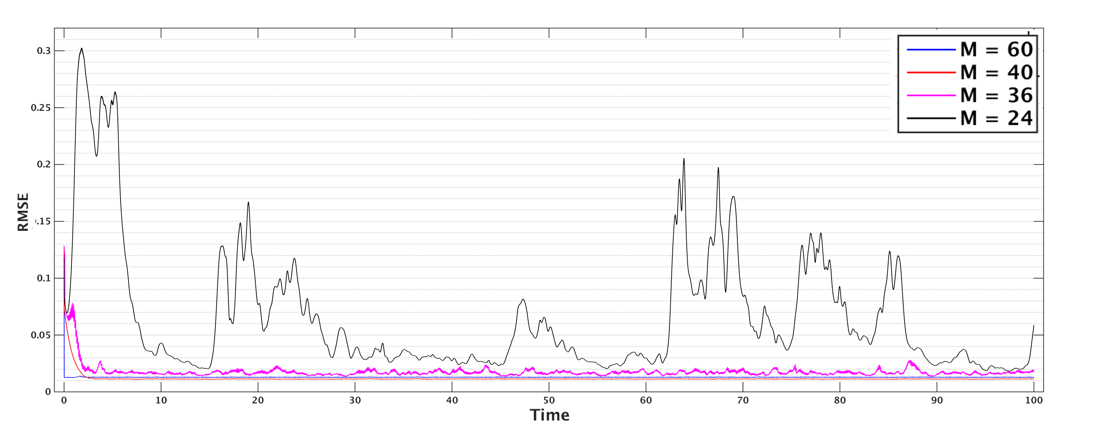
Figure 5.1: Fixed Observation Operator 3DVAR. Comparison with the case when $M=24$. RMSE value averaged over the trajectory for $M=24$ is $5.73\times 10^{-2}$.

Figure 5.2 shows the $\tiny{\rm RMSE}\,\,$for adaptive observation 3DVAR. In this case we notice that the error is consistently small, uniformly in time, with just $9$ or more modes observed. When $M=9$ ($15\%$ observed modes) the $\tiny{\rm RMSE}\,\,$averaged over the trajectory is $1.35\times 10^{-2}$ which again is of the order of the observational noise variance. For $M\geq 9$ the error is similar – see Figure 2(b). On the other hand, for smaller values of $M$ the error is not controlled as shown in Figure 2(a) where the $\tiny{\rm RMSE}\,\,$for $M=7$ is compared with that for $M=9;$ for $M=7$ it is an order of magnitude larger than for $M=9$. It is noteworthy that the number of observations necessary and sufficient for accurate reconstruction is approximately half the number of positive Lyapunov exponents.

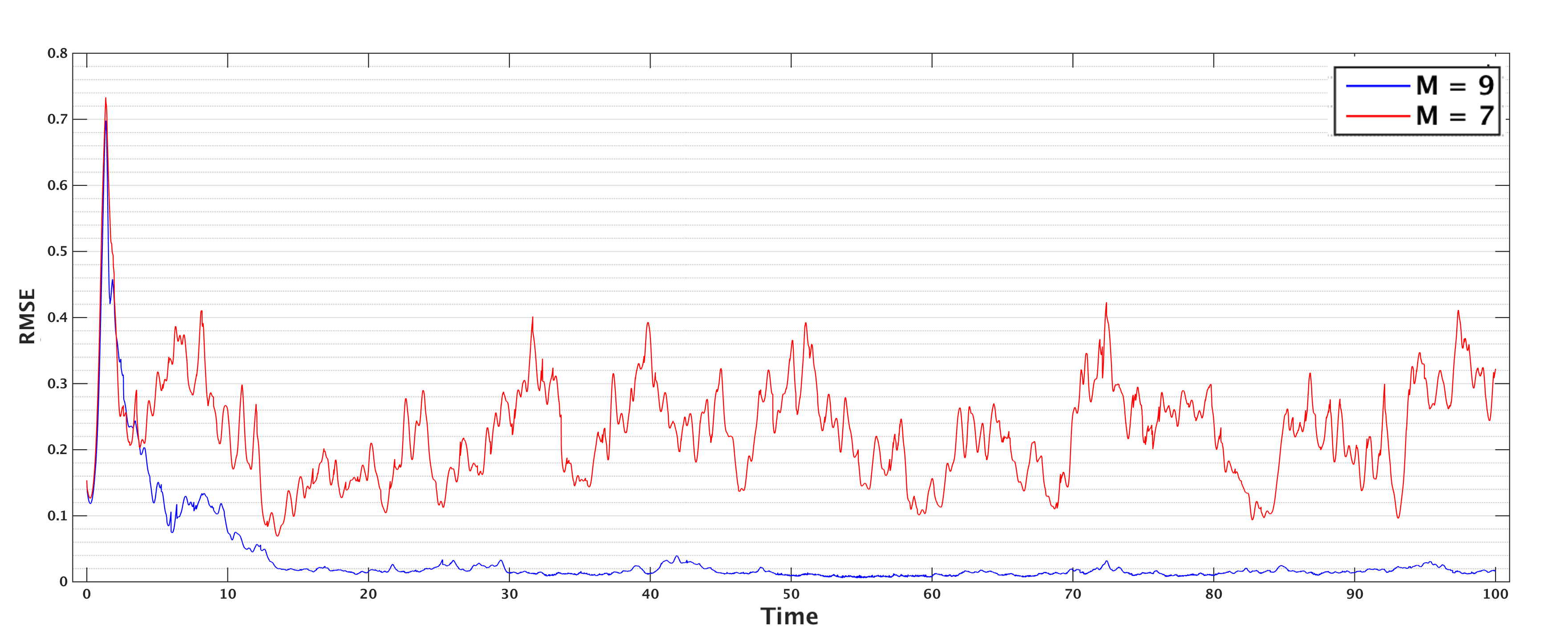
(a) Comparison of RMSE between M = 7 and M = 9. RMSE values averaged over trajectory are $2.25\times 10^{-1}$, $1.35\times 10^{-2}$ respectively.

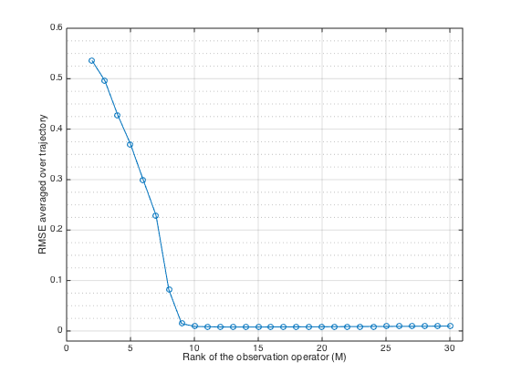
(b) Averaged RMSE for different choices of $M$

Figure 5.2: Adaptive Observation 3DVAR

5.2 Extended Kalman Filter

In the Extended Kalman Filter (ExKF) the approximate solution evolves according to the minimization principle (2.4) with $C_{k}$ chosen as a covariance matrix evolving in the forecast step according to the linearized dynamics, and in the assimilation stage updated according to Bayes’ rule based on a Gaussian observational error covariance. This gives the method

$$m_{k+1} = \Psi(m_{k})+G_{k+1}\Big{(}y_{k+1}-H_{k+1}\Psi({m}_{k})\Big{)},$$

$$\widehat{C}_{k+1} = D\Psi(m_{k})C_{k}D\Psi(m_{k})^{T},$$

$$C_{k+1} = (I_{J\times J}-G_{k+1}H_{k+1})\widehat{C}_{k+1},$$

$$G_{k+1} = \widehat{C}_{k+1}H_{k+1}^{T}(H_{k+1}\widehat{C}_{k+1}H_{k+1}^{T}+\Gamma)^{-1}.$$

We first consider the ExKF scheme with a fixed observation operator $H_{k}=H.$ We make two choices for $H$: the full rank identity operator and a partial observation operator given by (5.9) so that $40\%$ of the modes are observed. For the first case the filtering scheme is the standard ExKF with all the modes being observed. The approximate solution converges to the true solution and the error decreases rapidly as can be seen in the Figure 3(a). The $\tiny{\rm RMSE}\,\,$is $9.49\times 10^{-4}$ which is an order of magnitude smaller than the analogous error for the 3DVAR algorithm when fully observed which is, recall, $1.30\times 10^{-2}$. For the partial observations case with $M=24$ we see that again the approximate solution converges to the true underlying solution as shown in the Figure 3(b). Furthermore the solution given by the ExKF with $M=24$ is far more robust than for 3DVAR with this number of observations. The $\tiny{\rm RMSE}\,\,$is also lower for ExKF $(2.68\times 10^{-3})$ when compared with the 3DVAR scheme $(5.73\times 10^{-2})$.

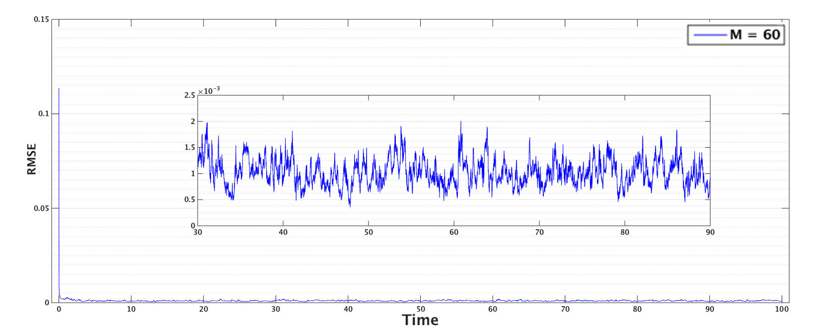
(a) Percentage of components observed = $100\%$. RMSE value averaged over trajectory $9.49\times 10^{-4}.$

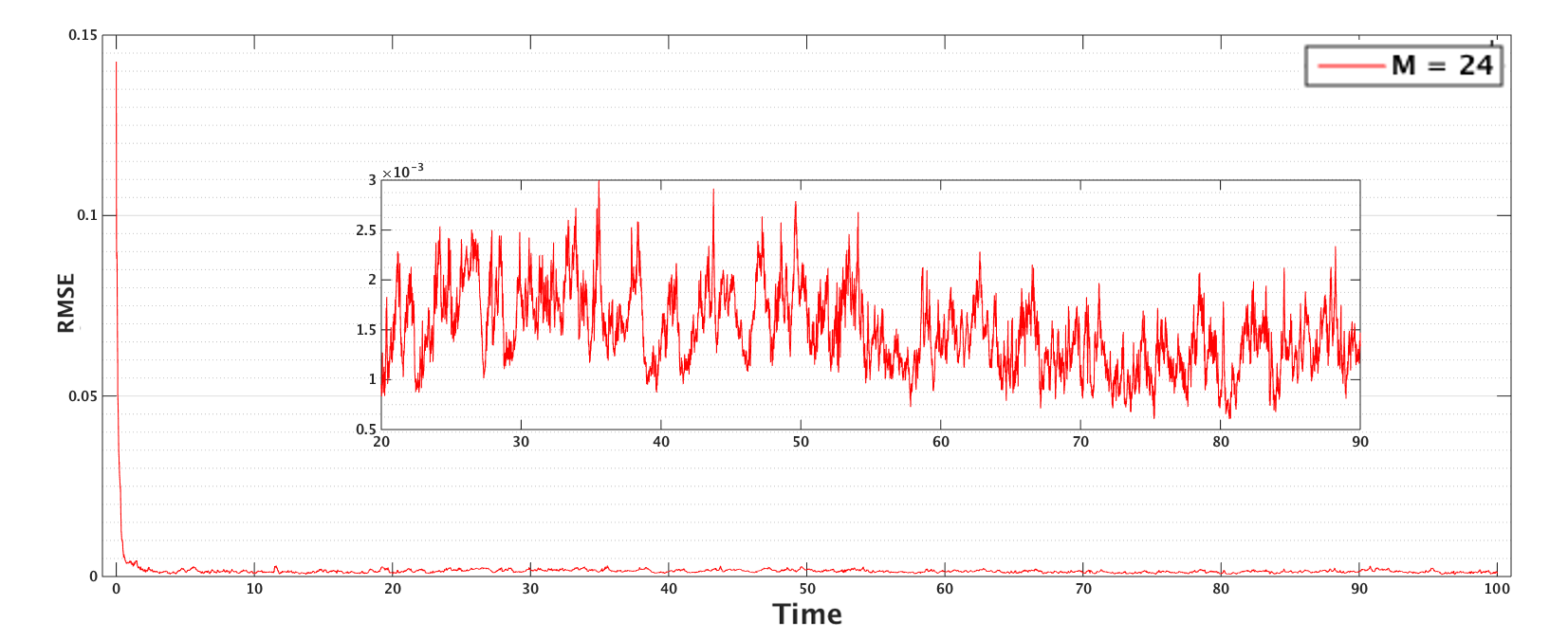
(b) Percentage of components observed = $40\%$. RMSE value averaged over trajectory $1.39\times 10^{-3}.$

Figure 5.3: Fixed Observation ExKF. The zoomed in figures shows the variability in RMSE between time $t=20$ and $t=90$.

We now turn to adaptive observation within the context of the ExKF. The Figure 5.4 shows that it is possible to obtain an $\tiny{\rm RMSE}\,\,$which is of the order of the observational error, and is robust over long time intervals, using only a $6$ dimensional observation space, improving marginally on the 3DVAR situation where $9$ dimensions were required to attain a similar level of accuracy.

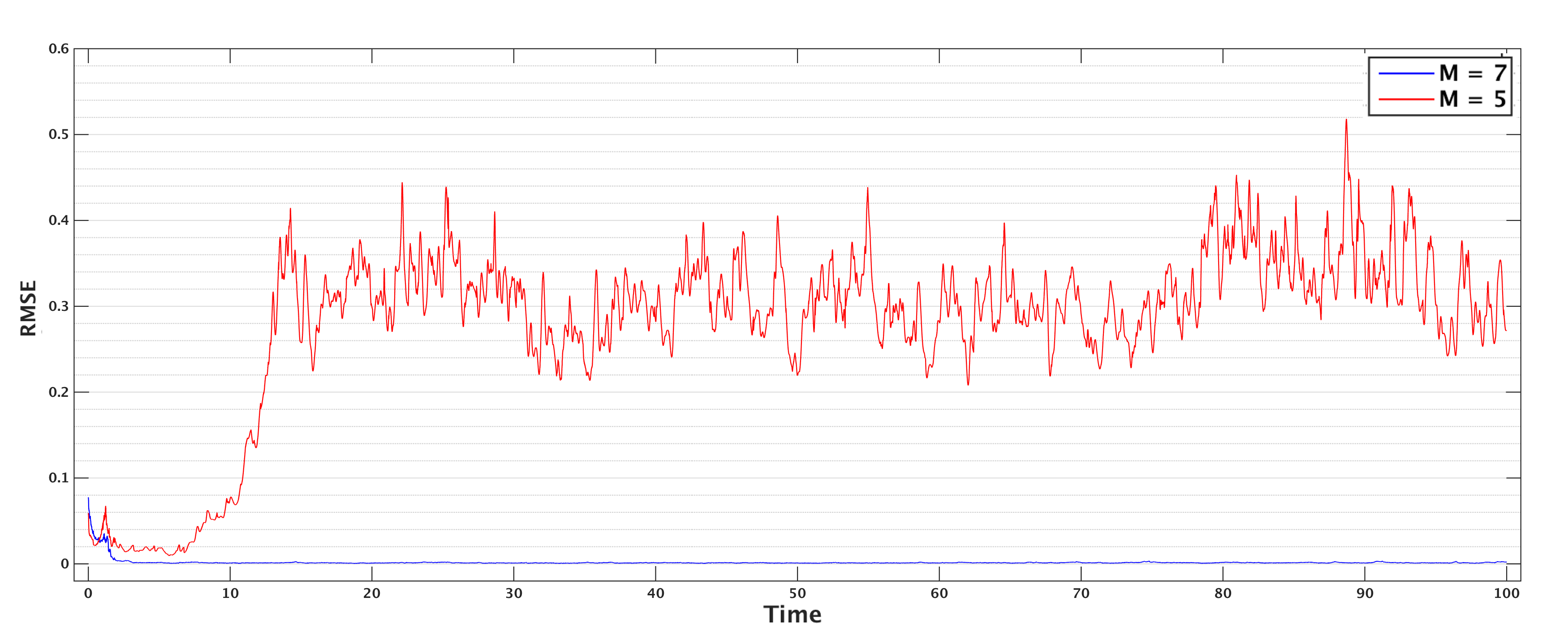
(a) Comparison of RMSE between M = 5 and M = 7. RMSE values averaged over trajectory are $2.84\times 10^{-1}$, $1.31\times 10^{-3}$ respectively.

(b) Averaged RMSE for different choices of $M$.

Figure 5.4: Adaptive Observation ExKF

The AUS scheme, proposed by Trevisan and co-workers [20, 19], is an ExKF method which operates by confining the analysis update to a subspace designed to capture the instabilities in the dynamics. This subspace is typically chosen as the span of the $M$ largest growth directions, where $M$ is the precomputed number of non-negative Lyapunov exponents.To estimate the unstable subspace one starts with $M$ orthogonal perturbation vectors and propagates them forward under the linearized dynamics in the forecast step to obtain a forecast covariance matrix $(\hat{C_{k}}).$ The perturbation vectors for the next assimilation cycle are provided by the square root of the covariance matrix $(C_{k})$ which can be computed via a suitable $M\times M$ transformation as shown in equations (11)-(15) of [19]. Under the assumption that the observational noise is sufficiently small that the truth of the exact model is close to the estimated mean and the discontinuity of the update is not too significant, it can be argued that the unstable subspace generated by the dominant Lyapunov vectors is preserved through the assimilation cycle. This has been illustrated numerically in [19] and references therein. That work also observes the phenomenon of reduced error in the AUS scheme as compared to the full assimilation, due to corruption by observational noise in stable directions in the latter case. Asymptotically this method with $H=I_{J\times J}$ behaves similarly to the adaptive ExKF with observation operator of rank $M$. To understand the intuition behind the AUS method we plot in Figure 5(a) the rank (computed by truncation to zero of eigenvalues below a threshold) of the covariance matrix $C_{k}$ from standard ExKF based on observing $60$ and $24$ modes. Notice that in both cases the rank approaches a value of $19$ or $20$ and that $19$ is the number of non-negative Lyapunov exponents. This means that the covariance is effectively zero in $40$ of the observed dimensions and that, as a consequence of the minimization principle (2.4), data will be ignored in the $40$ dimensions where the covariance is negligible. It is hence natural to simply confine the update step to the subspace of dimension $19$ given by the number of positive Lyapunov exponents, right from the outset. This is exactly what AUS does by reducing the rank of the error covariance matrix $C_{k}$. Numerical results are given in Figure 5(b) which shows the $\tiny{\rm RMSE}\,\,$over the trajectory for the ExKF-AUS assimilation scheme versus time for the observation operator $H=I_{J\times J}$. After initial transients the error is mostly of the numerical order of the observational noise. Occasional jumps outside this error bound are observed but the approximate solution converges to the true solution each time. The $\tiny{\rm RMSE}\,\,$for ExKF-AUS is $1.49\times 10^{-2}$. However, if the rank of the error covariance matrix $C_{0}$ in AUS is chosen to be less than the number of unstable modes for the underlying system, then the approximate solution does not converge to the true solution.

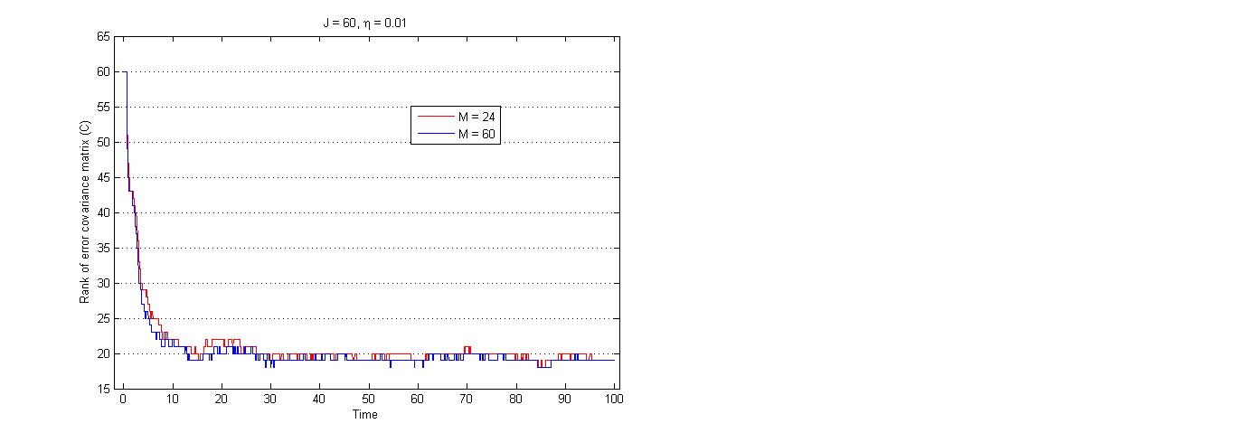
(a) Standard ExKF with $60$ and $24$ observed modes. The rank of the error covariance matrix $C_{k}$ decays to (approximately) the number of unstable Lyapunov modes in the underlying system, namely $19$.

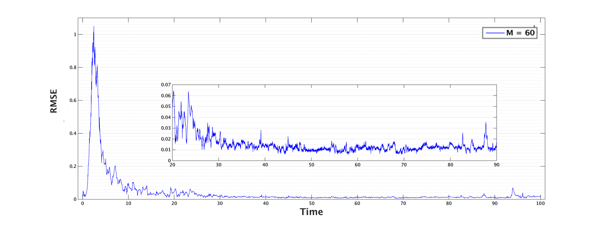
(b) RMSE value averaged over trajectory: $1.49\times 10^{-2}.$ The zoomed in figures shows the variability in RMSE between time $t=20$ and $t=90$. The rank of observation operator is chosen $M=60$.

Figure 5.5: Rank of error covariance and ExKF-Assimilation in Unstable Space

6 Conclusions

In this paper we have studied the long-time behaviour of filters for partially observed dissipative dynamical systems, using the Lorenz ’96 model as a canonical example. We have highlighted the connection to synchronization in dynamical systems, and shown that this synchronization theory, which applies to noise-free data, is robust to the addition of noise, in both the continuous and discrete time settings. In so doing we are studying the 3DVAR algorithm. In the context of the Lorenz ’96 model we have identified a fixed observation operator, based on observing 2/3 of the components of the signal’s vector, which is sufficient to ensure desirable long-time properties of the filter. However it is to be expected that, within the context of fixed observation operators, considerably fewer observations may be needed to ensure such desirable properties. Ideas from nonlinear control theory will be relevant in addressing this issue. We also studied adaptive observation operators, targeted to observe the directions of maximal growth within the local linearized dynamics. We demonstrated that with these adaptive observers, considerably fewer observations are required. We also made a connection between these adaptive observation operators, and the AUS methodology which is also based on the local linearized dynamics, but works by projecting within the model covariance operators of ExKF, whilst the observation operators themselves are fixed; thus the model covariances are adapted. Both adaptive observation operators and the AUS methodology show the potential for considerable computational savings in filtering, without loss of accuracy.

In conclusion our work highlights the role of ideas from dynamical systems in the rigorous analysis of filtering schemes and, through computational studies, shows the gap between theory and practice, demonstrating the need for further theoretical developments. We emphasize that the adaptive observation operator methods may not be implementable in practice on the high dimensional systems arising in, for example, meteorological applications. However, they provide conceptual insights into the development of improved algorithms and it is hence important to understand their properties.

Acknowledgements. AbS and DSA are supported by the EPSRC-MASDOC graduate training scheme. AMS is supported by EPSRC, ERC and ONR. KJHL is supported by King Abdullah University of Science and Technology, and is a member of the KAUST SRI-UQ Center.

Appendix: Proofs

Proof of Properties 3.1.

Properties 1, 2 and 3 are straightforward and we omit the proofs. We start showing 4. For any $u\in\mathbb{R}^{J}$ set

$$\|u\|_{\infty}=\underset{1\leq j\leq J}{\max}|u^{(j)}|$$

and recall that $|u|^{2}\geq\|u\|_{\infty}^{2}.$ Then, for $u,\tilde{u}\in\mathbb{R}^{J}$, and for $1\leq j\leq J$, we have that

$$2|B(u,\tilde{u})^{(j)}| \leq \|u\|_{\infty}(|\tilde{u}^{(j+1)}|+|\tilde{u}^{(j-2)}|)+\|\tilde{u}\|_{\infty}(|u^{(j+1)}|+|u^{(j-2)}|),$$

and so

$$4|B(u,\tilde{u})|^{2} \leq 2\|u\|^{2}_{\infty}\overset{J}{\underset{j=1}{\sum}}(|\tilde{u}^{(j+1)}|+|\tilde{u}^{(j-2)}|)^{2}+2\|\tilde{u}\|^{2}_{\infty}\overset{J}{\underset{j=1}{\sum}}(|u^{(j+1)}|+|u^{(j-2)}|)^{2}$$

$$\leq 8\|u\|^{2}_{\infty}|\tilde{u}|^{2}+8\|\tilde{u}\|^{2}_{\infty}|u|^{2}$$

$$\leq 16|u|^{2}|\tilde{u}|^{2}.$$

Hence

$$|B(u,\tilde{u})|\leq 2|u||\tilde{u}|.$$

For 5 we use rearrangement and periodicity of indices under summation as follows:

$$2\langle B(u,\tilde{u}),u\rangle = \overset{J}{\underset{j=1}{\sum}}\Big{(}u^{(j)}(u^{(j-1)}\tilde{u}^{(j+1)}+\tilde{u}^{(j-1)}u^{(j+1)}-\tilde{u}^{(j-1)}u^{(j-2)}-u^{(j-1)}\tilde{u}^{(j-2)})\Big{)}$$

$$= \overset{J}{\underset{j=1}{\sum}}(u^{(j)}u^{(j-1)}\tilde{u}^{(j+1)}-u^{(j)}\tilde{u}^{(j-1)}u^{(j-2)})$$

$$= \overset{J}{\underset{j=1}{\sum}}(u^{(j-1)}u^{(j-2)}\tilde{u}^{(j)}-u^{(j+1)}\tilde{u}^{(j)}u^{(j-1)})$$

$$= \overset{J}{\underset{j=1}{\sum}}\Big{(}\tilde{u}^{(j)}(u^{(j-1)}u^{(j-2)}-u^{(j+1)}u^{(j-1)})\Big{)}$$

$$= -\langle B(u,u),\tilde{u}\rangle.$$

∎

Proof of Proposition 3.2.

Taking the Euclidean inner product of $u(t)$ with equation (3.3) and using properties 1 and 2 we get

$$\frac{1}{2}\frac{\textrm{d}|u|^{2}}{\textrm{d}t}=-|u|^{2}+\langle f,u\rangle.$$

Using Young’s inequality for the last term gives

$$\frac{\textrm{d}|u|^{2}}{\textrm{d}t}+|u|^{2}\leq JF^{2}.$$

Therefore, using Gronwall’s lemma,

$$|u(t)|^{2}\leq|u_{0}|^{2}e^{-t}+JF^{2}(1-e^{-t}),$$

and the result follows. ∎

Proof of Property 4.5.

The first part is automatic since, if $q:=Qu$, then for all $j$ either $q^{(j-1)}=0$ or $q^{(j-2)}=q^{(j+1)}=0$. Since $B(Qu,Qu)=0$ and $B(\cdot,\cdot)$ is a bilinear operator we can write

$$B(u,u) = B(Pu+Qu,Pu+Qu)$$

$$= B(Pu,Pu)+2B(Pu,Qu).$$

Now using property 4, and the fact that there is $c>0$ such that $|Pu|+2|Qu|\leq\frac{c}{2}|u|,$

$$|\langle B(u,u),\tilde{u}\rangle| \leq |B(u,u)||\tilde{u}|$$

$$\leq |B(Pu,Pu)+2B(Pu,Qu)||\tilde{u}|$$

$$\leq 2|Pu||\tilde{u}|(|Pu|+2|Qu|)$$

$$\leq c|Pu||\tilde{u}||u|.$$

∎

Proof of Theorem 4.7.

Define the error in the approximate solution as $\delta=m-v=q-Qv$. Note that $Q\delta=\delta$. The error satisfies the following equation

$$Q\frac{\textrm{d}\delta}{\textrm{d}t}+Q\delta+Q\big{(}B(Pv+q,Pv+q)-B(v,v)\big{)}=0.$$

Splitting $v=Pv+Qv$ and noting, from Properties 4.5, that $B(Qv,Qv)=0$ and $B(q,q)=0$, yields

$$\frac{\textrm{d}Q\delta}{\textrm{d}t}+Q\delta+2QB(Pv,Q\delta)=0.$$

Taking the inner product with $Q\delta$ gives

$$\frac{1}{2}\frac{\textrm{d}|Q\delta|^{2}}{\textrm{d}t}+|Q\delta|^{2}+2\langle B(Pv,Q\delta),Q\delta\rangle=0.$$

Note that from the Properties 3.1, 3 and 5, and Property 4.5, we have

$$2\langle B(u,Q\delta),Q\delta\rangle = -\langle B(Q\delta,Q\delta),u\rangle$$

$$= 0.$$

Thus since $Q\delta=\delta$ we have

$$\frac{\textrm{d}|\delta|^{2}}{\textrm{d}t}+2|\delta|^{2}=0,$$

and so

$$|\delta(t)|^{2}=|\delta(0)|^{2}e^{-2t}.$$

As $t\rightarrow\infty$ the error $\delta(t)\rightarrow 0$. ∎

Proof of Theorem 4.8.

From (4.6) and (4.7)

$$\frac{\textrm{d}m}{\textrm{d}t}=\mathcal{F}(m)+\frac{1}{\eta}\Big{(}Pv+\epsilon P\frac{\textrm{d}w}{\textrm{d}t}-Pm\Big{)}.$$

Thus

$$\frac{\textrm{d}m}{\textrm{d}t}=-m-B(m,m)+f+\frac{1}{\eta}P(v-m)+\frac{\epsilon}{\eta}P\frac{\textrm{d}w}{\textrm{d}t}.$$

The signal is given by

$$\frac{\textrm{d}v}{\textrm{d}t}=-v-B(v,v)+f,$$

and so the error $\delta=m-v$ satisfies

$$\frac{\textrm{d}\delta}{\textrm{d}t}=-\delta-2B(v,\delta)-B(\delta,\delta)-\frac{1}{\eta}P\delta+\frac{\epsilon}{\eta}P\frac{\textrm{d}w}{\textrm{d}t}.$$

Lemma 6.13 below, Properties 3.1 and Itó’s formula give

$$\frac{1}{2}\textrm{d}|\delta|^{2}+\Big{(}1-\frac{c^{2}K\eta}{4}\Big{)}|\delta|^{2}{\textrm{d}t}\leq\frac{\epsilon}{\eta}\langle P\textrm{d}w,\delta\rangle+\frac{J}{3}\frac{\epsilon^{2}}{\eta^{2}}{\textrm{d}t}.$$

Integrating and taking expectations

$$\frac{\textrm{d}\mathbb{E}{|\delta|}^{2}}{\textrm{d}t}\leq-\lambda\mathbb{E}{|\delta|}^{2}+\frac{2J\epsilon^{2}}{3\eta^{2}}.$$

Use of the Gronwall inequality gives the desired result. ∎

We now turn to discrete-time data assimilation, where the following lemma plays an important role:

Lemma 6.12.

Consider the Lorenz ’96 model (3.3) with $F>0$ and $J\geq 3.$ Let $v$ and $u$ be two solutions in $[t_{k},t_{k+1}),$ with $v(t_{k})\in\mathcal{B}.$ Then there exists a $\beta\in\mathbb{R}$ such that

$$|u(t)-v(t)|^{2}\leq|u(t_{k})-v(t_{k})|^{2}e^{\beta(t-t_{k})}\quad t\in[t_{k},t_{k+1}).$$

Proof.

Let $\delta=m-v.$ Then $\delta$ satisfies

$$\frac{1}{2}\frac{\textrm{d}|\delta|^{2}}{\textrm{d}t}+|\delta|^{2}+2\langle B(v,\delta),\delta\rangle+\langle B(\delta,\delta),\delta\rangle=0$$ (6.1)

so that, by Property 3.1, item 2,

$$\frac{1}{2}\frac{\textrm{d}|\delta|^{2}}{\textrm{d}t}+|\delta|^{2}-2|\langle B(v,\delta),\delta\rangle|\leq 0.$$

Using Properties 3.1 items 4 and 5 gives $|\langle B(v,\delta),\delta\rangle|\leq K^{\frac{1}{2}}|\delta|^{2}$, where $K$ is defined in Proposition 3.2, so that

$$\frac{1}{2}\frac{\textrm{d}|\delta|^{2}}{\textrm{d}t}\leq(2K^{\frac{1}{2}}-1)|\delta|^{2}.$$

Integrating the differential inequality gives

$$|\delta(t)|^{2}\leq|\delta(t_{k})|^{2}e^{\beta(t-t_{k})}.$$ (6.2)

∎

Note if $F<\frac{1}{2\sqrt{2}J}$ then $\beta=2(2K^{\frac{1}{2}}-1)<0$ and the subsequent analysis may be significantly simplified. Thus we assume in what follows that $F\geq\frac{1}{2\sqrt{2}J}$ so that $\beta\geq 0.$ Lemma 6.12 gives an estimate on the growth of the error in the forecast step. Our aim now is to show that this growth can be controlled by observing $Pv$ discretely in time. It will be required that the time $h$ between observations is sufficiently small.

To ease the notation we introduce three functions that will be used in the proofs of Theorems 4.5 and 4.10. Namely we define, for $t>0,$

$$A_{1}(t):=\frac{16K}{\beta}(e^{\beta t}-1)+\frac{4R_{0}^{2}}{2\beta}(e^{2\beta t}-1),$$ (6.3)

$$B_{1}(t):=\frac{16c^{2}K^{2}}{\beta}\left[\frac{e^{\beta t}-e^{-t}}{\beta+1}-(1-e^{-t})\right]+e^{-t}+\frac{4c^{2}KR_{0}^{2}}{2\beta}\left[\frac{e^{2\beta t}-e^{-t}}{2\beta+1}-(1-e^{-t})\right],$$ (6.4)

and

$$B_{2}(t):=c^{2}K\{1-e^{-t}\}.$$ (6.5)

Here and in what follows $c$, $\beta$ and $K$ are as in Property 4.5, Lemma 6.12 and Proposition 3.2. We will use two different norms in $\mathbb{R}^{J}$ to prove the theorems that follow. In each case, the constant $R_{0}>0$ above quantifies the size of the initial error, measured in the relevant norm for the result at hand.

Proof of Theorem 4.9.

Define the error $\delta=m-v.$ Subtracting equation (4.3) from equation (4.10) gives

$$\frac{\textrm{d}\delta}{\textrm{d}t}+\delta+2B(v,\delta)+B(\delta,\delta)=0,\quad t\in(t_{k},t_{k+1}),$$ (6.6a)

$$\delta(t_{k})=Q\delta(t_{k}^{-})$$ (6.6b)

where $\delta(t_{k+1}^{-}):=\lim_{t\uparrow t_{k+1}}\delta(t)$ as defined in section 4.2.1. Notice that $B_{1}(0)=1$ and $B_{1}^{\prime}(0)=-1$, so that there is $h^{*}>0$ with the property that $B_{1}(h)\in(0,1)$ for all $h\in(0,h^{*}].$ Fix any such assimilation time $h$ and denote $\gamma=B_{1}(h)\in(0,1).$ Let $R_{0}:=|\delta_{0}|$. We show by induction that, for every $k,$ $|\delta_{k}|^{2}\leq\gamma^{k}R_{0}^{2}.$ We suppose that it is true for $k$ and we prove it for $k+1.$

Taking the inner product of $P\delta$ with the equation (6.6) gives

$$\frac{1}{2}\frac{\textrm{d}|P\delta|^{2}}{\textrm{d}t}+|P\delta|^{2}+2\langle B(v,\delta),P\delta\rangle+\langle B(\delta,\delta),P\delta\rangle=0$$

so that, by Property 3.1, item 4,

$$\frac{1}{2}\frac{\textrm{d}|P\delta|^{2}}{\textrm{d}t}+|P\delta|^{2}\leq 4|v||\delta||P\delta|+2|\delta|^{2}|P\delta|.$$

By the inductive hypothesis we have $|\delta_{k}|^{2}\leq R_{0}^{2}$ since $\gamma\in(0,1)$. Shifting the time origin by setting $\tau:=t-t_{k}$ and using Lemma 6.12 gives

$$\frac{1}{2}\frac{\textrm{d}|P\delta|^{2}}{\textrm{d}\tau}+|P\delta|^{2} \leq 4K^{\frac{1}{2}}|\delta||P\delta|+2|\delta_{k}|e^{\frac{\beta\tau}{2}}|\delta||P\delta|$$

$$\leq 4K^{\frac{1}{2}}|\delta||P\delta|+2R_{0}e^{\frac{\beta\tau}{2}}|\delta||P\delta|.$$ (6.7)

Applying Young’s inequality to each term on the right-hand side we obtain

$$\frac{\textrm{d}|P\delta|^{2}}{\textrm{d}\tau}\leq 16K|\delta|^{2}+4R_{0}^{2}e^{\beta\tau}|\delta|^{2}.$$ (6.8)

Integrating from $0$ to $s$, where $s\in(0,h)$, gives

$$|P\delta(s)|^{2} \leq A_{1}(s)|\delta_{k}|^{2}.$$ (6.9)

Now again consider the equation (6.1) using Property 3.1 item 5 to obtain

$$\frac{1}{2}\frac{\textrm{d}|\delta|^{2}}{\textrm{d}\tau}+|\delta|^{2}-|\langle B(\delta,\delta),v\rangle|\leq 0.$$

Using Property 4.5 and Young’s inequality yields

$$\frac{1}{2}\frac{\textrm{d}|\delta|^{2}}{\textrm{d}\tau}+|\delta|^{2} \leq c|v||\delta||P\delta|$$ (6.10)

$$\leq cK^{\frac{1}{2}}|\delta||P\delta|$$

$$\leq \frac{|\delta|^{2}}{2}+\frac{c^{2}K}{2}|P\delta|^{2}.$$

Employing the bound (6.9) then gives

$$\frac{\textrm{d}|\delta|^{2}}{\textrm{d}\tau}+|\delta|^{2}\leq\left(\frac{16c^{2}K^{2}}{\beta}(e^{\beta\tau}-1)+\frac{4c^{2}KR_{0}^{2}}{2\beta}(e^{2\beta\tau}-1)\right)|\delta_{k}|^{2}.$$

Therefore, upon using Gronwall’s lemma,

$$|\delta(s)|^{2}\leq B_{1}(s)|\delta_{k}|^{2}.$$

It follows that

$$|\delta_{k+1}|^{2}\leq\gamma|\delta_{k}|^{2}\leq\gamma^{k+1}R_{0}^{2},$$

and the induction (and hence the proof) is complete. ∎

Proof of Theorem 4.10.

We define the error process $\delta(t)$ as follows:

$$\delta(t)=\left\{\begin{array}[]{c}\delta_{k}:=m_{k}-v(t)\quad\textrm{if}\>\>t=t_{k}\\ \Psi(m_{k},t-t_{k})-v(t)\quad\textrm{if}\>\>t\in(t_{k},t_{k+1}).\\ \end{array}\right.$$ (6.11)

Observe that $\delta$ is discontinuous at times $t_{k}$ which are multiples of $h$, since $m_{k+1}\neq\Psi(m_{k};h).$ Subtracting (4.12) from (4.11) we obtain

$${\delta_{k+1}} =\delta(t_{k+1})=\left(\frac{\eta}{1+\eta}P+Q\right)\delta(t^{-}_{k+1})+\frac{1}{1+\eta}{\nu_{k+1}},$$ (6.12)

$$P\delta_{k+1} =\frac{\eta}{1+\eta}P\delta(t^{-}_{k+1})+\frac{1}{1+\eta}\nu_{k+1},$$ (6.13)

where $\delta(t_{k+1}^{-}):=\lim_{t\uparrow t_{k+1}}\delta(t)$ as defined above and in section 4.2.1.

Let $A_{1}(\cdot)$, $B_{1}(\cdot)$ and $B_{2}(\cdot)$ be as in (6.3, 6.4, 6.5), and set

$$M_{1}(t):= \frac{2\eta}{1+\eta}\sqrt{A_{1}(t)}+\sqrt{B_{1}(t)},$$

$$M_{2}(t):= \frac{2\eta}{1+\eta}+\sqrt{B_{2}(t)}.$$

Since $A_{1}(0)=0,B_{1}(0)=1,$ $B_{2}(0)=0$ and

$$\frac{d}{dt}\sqrt{B_{1}(t)}\Big{|}_{t=0}=-1/2<0$$

it is possible to find $h,\eta>0$ small such that

$$M_{2}(h)<M_{1}(h)=:\alpha<1.$$

Let $R_{0}=\|\delta_{0}\|$. We show by induction that for such $h$ and $\eta,$ and provided that $\epsilon$ is small enough so that

$$\alpha R_{0}+2\epsilon<R_{0},$$

we have that $\|\delta_{k}\|\leq R_{0}$ for all $k.$ Suppose for induction that it is true for $k.$ Then $|\delta_{k}|\leq\|\delta_{k}\|\leq R_{0}$ and we can apply (after shifting time as before) Lemma 6.14 below to obtain that

$$|P\delta(t_{k}+t))|\leq\sqrt{A_{1}(t)|\delta_{k}|^{2}+|P\delta_{k}|^{2}}\leq\sqrt{A_{1}(t)}|\delta_{k}|+|P\delta_{k}|$$

and

$$|\delta(t_{k}+t)|\leq\sqrt{B_{1}(t)|\delta_{k}|^{2}+B_{2}(t)|P\delta_{k}|^{2}}\leq\sqrt{B_{1}(t)}|\delta_{k}|+\sqrt{B_{2}(t)}|P\delta_{k}|.$$

Therefore, combining (6.12) and (6.13), and then using the two previous inequalities, we obtain that

$$|P\delta_{k+1}|+|\delta_{k+1}| \leq\frac{2\eta}{1+\eta}|P\delta(t^{-}_{k+1})|+|\delta(t^{-}_{k+1})|+\frac{2}{1+\eta}|\nu_{k+1}|$$

$$\leq\left(\frac{2\eta}{1+\eta}\sqrt{A_{1}(h)}+\sqrt{B_{1}(h)}\right)|\delta_{k}|+\left(\frac{2\eta}{1+\eta}+\sqrt{B_{2}(h)}\right)|P\delta_{k}|+2\epsilon$$

$$=M_{1}(h)|\delta_{k}|+M_{2}(h)|P\delta_{k}|+2\epsilon.$$

Since $M_{2}(h)<M_{1}(h)=\alpha$ we deduce that

$$\|\delta_{k+1}\|\leq\alpha\|\delta_{k}\|+2\epsilon,$$

which proves (4.13). Furthermore, the induction is complete, since

$$\|\delta_{k+1}\|\leq\alpha\|\delta_{k}\|+2\epsilon\leq\alpha R_{0}+2\epsilon\leq R_{0}.$$

∎

Lemma 6.13.

Let $v\in\mathcal{B}.$ Then, for any $\delta,$

$$\langle\delta+2B(v,\delta)+B(\delta,\delta)+\frac{1}{\eta}P\delta,\delta\rangle\geq\Big{(}1-\frac{c^{2}K\eta}{4}\Big{)}|\delta|^{2}.$$

Proof.

Use of Property 3.1, items 3 and 5, together with Property 4.5, shows that

$$\langle\delta+2B(v,\delta)+B(\delta,\delta)+\frac{1}{\eta}P\delta,\delta\rangle = |\delta|^{2}+2\langle B(v,\delta),\delta\rangle+\langle B(\delta,\delta),\delta\rangle+\langle\frac{1}{\eta}P\delta,\delta\rangle$$

$$= |\delta|^{2}-\langle B(\delta,\delta),v\rangle+\langle\frac{1}{\eta}P\delta,\delta\rangle$$

$$\geq |\delta|^{2}-cK^{\frac{1}{2}}|\delta||P\delta|+\frac{1}{\eta}|P\delta|^{2}$$

$$\geq |\delta|^{2}-\frac{\theta|\delta|^{2}}{2}-\frac{c^{2}K|P\delta|^{2}}{2\theta}+\frac{1}{\eta}|P\delta|^{2}.$$

Now choosing $\theta=\frac{c^{2}K\eta}{2}$ establishes the claim.

∎

Lemma 6.14.

In the setting of Theorem 4.10, for $t\in[0,h)$ and $R_{0}:=\|\delta_{0}\|$ we have

$$|P\delta(t)|^{2}\leq A_{1}(t)|\delta_{0}|^{2}+|P\delta_{0}|^{2}$$ (6.14)

and

$$|\delta(t)|^{2}\leq B_{1}(t)|\delta_{0}|^{2}+B_{2}(t)|P\delta_{0}|^{2},$$ (6.15)

where the error $\delta$ is defined as in (6.11) and $A_{1},B_{1}$ and $B_{2}$ are given by (6.3, 6.4, 6.5).

Proof.

As in equation (6.8) we have

$$\frac{\textrm{d}|P\delta|^{2}}{\textrm{d}t}\leq 16K|\delta|^{2}+4R_{0}^{2}e^{\beta t}|\delta|^{2}.$$

On integrating from $0$ to $t$ as before, and noting that now $P\delta_{0}\neq 0$ in general, we obtain

$$|P\delta(t)|^{2}\leq\left(\frac{16K}{\beta}\{e^{\beta t}-1\}+\frac{4R_{0}^{2}}{2\beta}\{e^{2\beta t}-1\}\right)|\delta_{0}|^{2}+|P\delta_{0}|^{2},$$

which proves (6.14).

For the second inequality recall the bound (6.10)

$$\frac{1}{2}\frac{\textrm{d}|\delta|^{2}}{\textrm{d}t}+|\delta|^{2}\leq\frac{|\delta|^{2}}{2}+\frac{c^{2}K}{2}|P\delta|^{2},$$

and combine it with (6.14) to get

$$\frac{\textrm{d}|\delta|^{2}}{\textrm{d}t}+|\delta|^{2}\leq\left(\frac{16c^{2}K^{2}}{\beta}\{e^{\beta t}-1\}+\frac{4c^{2}KR_{0}^{2}}{2\beta}\{e^{2\beta t}-1\}\right)|\delta_{0}|^{2}+c^{2}K|P\delta_{0}|^{2}.$$

Applying Gronwall’s inequality yields (6.15). ∎

References

- [1] H.D.I. Abarbanel. Predicting the Future: Completing Models of Observed Complex Systems. Springer. Series: Understanding Complex Systems, 2013.
- [2] A. Azouani, E. Olson, and E.S. Titi. Continuous data assimilation using general interpolant observables. Journal of Nonlinear Science, 24:277–304, 2014.
- [3] G. Benettin, L. Galgani, and J.M. Strelcyn. Kolmogorov entropy and numerical experiments. Phys. Rev. A, 14:2338–2345, Dec 1976.
- [4] A. Bennett. Inverse Modeling of the Ocean and Atmosphere. Cambridge University Press, 2003.
- [5] D. Bloemker, K.J.H. Law, A.M. Stuart, and K.C. Zygalakis. Accuracy and stability of the continuous-time 3DVAR filter for the navier-stokes equation. Nonlinearity, 2014.
- [6] C.E.A. Brett, K.F. Lam, K.J.H. Law, D.S. McCormick, M.R. Scott, and A.M. Stuart. Accuracy and stability of filters for dissipative pdes. PhysicaD: Nonlinear Phenomena, 2013.
- [7] K. Hayden, E. Olson, and E.S. Titi. Discrete data assimilation in the Lorenz and 2d Navier-Stokes equations. Physica D: Nonlinear Phenomena, pages 1416–1425, 2011.
- [8] E. Kalnay. Atmospheric Modeling, Data Assimilation and Predictability. Cambridge University Press, 2003.
- [9] M. Kostuk. Synchronization and statistical methods for the data assimilation of HVc neuron models. PhD thesis, University of California, San Diego, 2012.
- [10] K.J.H. Law, A. Shukla, and A.M. Stuart. Analysis of the 3dvar filter for the partially observed lorenz ’63 model. Discrete and Continuous Dynamical Systems A, 34:1061–1078, 2014.
- [11] K.J.H. Law, A.M. Stuart, and K.C. Zygalakis. Data Assimilation: A Mathematical Introduction. Lecture Notes, 2014.
- [12] E.N. Lorenz and K.A. Emanuel. Optimal sites for supplementary weather observations: Simulation with a small model. Journal of the Atmospheric Sciences, 55:399–414, 1998.
- [13] A. Majda and J. Harlim. Filtering Complex Turbulent Systems. Cambridge University Press, 2012.
- [14] D. Oliver, A. Reynolds, and N. Liu. Inverse Theory for Petroleum Reservoir Characterization and History Matching. Cambridge University Press, 2008.
- [15] E. Olson and E. Titi. Determining modes for continuous data assimilation in 2d turbulence. Journal of Statistical Physics, 113:799–840, 2003.
- [16] E. Ott, B.R. Hunt, I. Szunyogh, A.V. Zimin, E.J. Kostelich, M. Corazza, E. Kalnay, D.J. Patil, and J.A. Yorke. A local ensemble Kalman filter for atmospheric data assimilation. Tellus A, 56(5):415–428, 2004.
- [17] T. Tarn and Y. Rasis. Observers for nonlinear stochastic systems. Automatic Control, IEEE Transactions, 21(4):441–488, 1976.
- [18] R. Temam. Infinite-Dimensional Dynamical Systems in Mechanics and Physics, volume 68 of Applied Mathematical Sciences. Springer-Verlag, New York, second edition, 1997.
- [19] A. Trevisan and L. Palatella. On the Kalman Filter error covariance collapse into the unstable subspace. Nonlinear Processes in Geophysics, 18:243–250, 2011.
- [20] A. Trevisan and F. Uboldi. Assimilation of standard and targeted observations within the unstable subspace of the observation analysis forecast cycle system. Journal of the Atmospheric Sciences, 61(1):103–113, 2004.