A Spitzer Five-Band Analysis of the Jupiter-Sized Planet TrES-1

Abstract

With an equilibrium temperature of 1200 K, TrES-1 is one of the coolest hot Jupiters observed by Spitzer. It was also the first planet discovered by any transit survey and one of the first exoplanets from which thermal emission was directly observed. We analyzed all Spitzer eclipse and transit data for TrES-1 and obtained its eclipse depths and brightness temperatures in the 3.6 m (0.083% $\pm$ 0.024%, 1270 $\pm$ 110 K), 4.5 m (0.094% $\pm$ 0.024%, 1126 $\pm$ 90 K), 5.8 m (0.162% $\pm$ 0.042%, 1205 $\pm$ 130 K), 8.0 m (0.213% $\pm$ 0.042%, 1190 $\pm$ 130 K), and 16 m (0.33% $\pm$ 0.12%, 1270 $\pm$ 310 K) bands. The eclipse depths can be explained, within 1$\sigma$ errors, by a standard atmospheric model with solar abundance composition in chemical equilibrium, with or without a thermal inversion. The combined analysis of the transit, eclipse, and radial-velocity ephemerides gives an eccentricity $e=0.033^{+0.015}_{-0.031}$, consistent with a circular orbit. Since TrES-1’s eclipses have low signal-to-noise ratios, we implemented optimal photometry and differential-evolution Markov-chain Monte Carlo (MCMC) algorithms in our Photometry for Orbits, Eclipses, and Transits (POET) pipeline. Benefits include higher photometric precision and $\sim$10 times faster MCMC convergence, with better exploration of the phase space and no manual parameter tuning.

1. INTRODUCTION

Transiting exoplanets offer the valuable chance to measure the light emitted from the planet directly. In the infrared, the eclipse depth of an occultation light curve (when the planet passes behind its host star) constrains the thermal emission from the planet. Furthermore, multiple-band detections allow us to characterize the atmosphere of the planet (e.g., Seager & Deming 2010). Since the first detections of exoplanet occultations—TrES-1 (Charbonneau et al. 2005) and HD 298458b (Deming et al. 2005)—there have been several dozen occultations observed. However, to detect an occultation requires an exhaustive data analysis, since the the planet-to-star flux ratios typically lie below $10^{-3}$. For example, for the Spitzer Space Telescope, these flux ratios are lower than the instrument’s photometric stability criteria (Fazio et al. 2004). In this paper we analyze Spitzer follow-up observations of TrES-1, highlighting improvement in light-curve data analysis over the past decade.

TrES-1 was the first exoplanet discovered by a wide-field transit survey (Alonso et al. 2004). Its host is a typical K0 thin-disk star (Santos et al. 2006a) with solar metallicity (Laughlin et al. 2005, Santos et al. 2006b, Sozzetti et al. 2006), effective temperature $T_{\rm eff}=5230\pm 50$ K, mass $M_{*}=0.878\pm 0.040$ solar masses ($M_{\odot}$), and radius $R_{*}=0.807\pm 0.017$ solar radii ($R_{\odot}$, Torres et al. 2008). Steffen & Agol (2005) dismissed additional companions (with $M>M_{\oplus}$). Charbonneau et al. (2005) detected the secondary eclipse in the 4.5 and 8.0 m Spitzer bands. Knutson et al. (2007) attempted ground-based eclipse observations in the L band (2.9 to 4.3 m), but did not detect the eclipse.

The TrES-1 system has been repeatedly observed during transit from ground-based telescopes (Narita et al. 2007, Raetz et al. 2009, Vaňko et al. 2009, Rabus et al. 2009, Hrudková et al. 2009, Sada et al. 2012) and from the Hubble Space Telescope (Charbonneau et al. 2007). The analyses of the cumulative data (Butler et al. 2006, Southworth 2008, 2009, Torres et al. 2008) agree (within error bars) that the planet has a mass of $M_{p}=0.752\pm 0.047$ Jupiter masses ($M_{\rm Jup}$), a radius $R_{p}=1.067\pm 0.022$ Jupiter radii ($R_{\rm Jup}$), and a circular, 3.03 day orbit, whereas Winn et al. (2007) provided accurate details of the transit light-curve shape. Recently, an adaptive-optics imaging survey (Adams et al. 2013) revealed that TrES-1 has a faint background stellar companion ($\Delta$mag = 7.68 in the Ks band, or 0.08% of the host’s flux) separated by 2.31″ (1.9 and 1.3 Spitzer pixels at 3.6–8 m and at 16 m, repectively). The companion’s type is unknown.

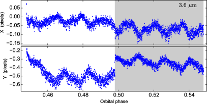
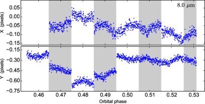
Figure 1.— Left: TrES-1’s $x$ (top) and $y$ (bottom) position on the detector at 3.6 m vs. orbital phase. The coordinate origin denotes the center of the nearest pixel. The shaded/unshaded areas mark different AORs. The ($\sim 0.1$ pixels) pointing offsets are clear, as well as the usual hour-long pointing oscillation and point-to-point jitter ($\sim 0.01$ pixels). Right: Same as the left panel, but for the 8.0 m light curve. The 5.8 and 4.5 m datasets were observed simultaneously with the 3.6 and 8.0 m bands, respectively; hence, their pointing correlates with the ones shown.

This paper analyzes all Spitzer eclipse and transit data for TrES-1 to constrain the planet’s orbit, atmospheric thermal profile, and chemical abundances. TrES-1’s eclipse has an inherently low signal-to-noise ratio (S/N). Additionally, as one of the earliest Spitzer observations, the data did not follow the best observing practices developed over the years. We take this opportunity to present the latest developments in our Photometry for Orbits, Eclipses, and Transits (POET) pipeline (Stevenson et al. 2010, 2012a, 2012b, Campo et al. 2011, Nymeyer et al. 2011, Cubillos et al. 2013) and demonstrate its robustness on low S/N data. We have implemented the differential-evolution Markov-chain Monte Carlo algorithm (DEMC, ter Braak 2006), which explores the parameter phase space more efficiently than the typically-used Metropolis Random Walk with a multivariate Gaussian distribution as the proposal distribution. We also test and compare multiple centering (Gaussian fit, center of light, PSF fit, and least asymmetry) and photometry (aperture and optimal) routines.

Section 2 describes the Spitzer observations. Section 3 outlines our data analysis pipeline. Section 4 presents our orbital analysis. Section 5 shows the constraints that our eclipse measurements place on TrES-1’s atmospheric properties. Finally, section 6 states our conclusions.

2. OBSERVATIONS

We analyzed eight light curves of TrES-1 from six Spitzer visits (obtained during the cryogenic mission): a simultaneous eclipse observation in the 4.5 and 8.0 m Infrared Array Camera (IRAC) bands (PI Charbonneau, program ID 227, full-array mode), a simultaneous eclipse observation in the 3.6 and 5.8 m IRAC bands (PI Charbonneau, program ID 20523, full-array), three consecutive eclipses in the 16 m Infrared Spectrograph (IRS) blue peak-up array, and one transit visit at 16 m (PI Harrington, program ID 20605). Table 1 shows the Spitzer band, date, total duration, frame exposure time, and Spitzer pipeline of each observation.

Table 1 Observation Information

Event	Band	Observation	Duration	Exp. time	Spitzer
	m	date	hours	seconds	pipeline
Eclipse	3.6	2005 Sep 17	7.27	01.2	S18.18.0
Eclipse	4.5	2004 Oct 30	5.56	10.4	S18.18.0
Eclipse	5.8	2005 Sep 17	7.27	10.4	S18.18.0
Eclipse	8.0	2004 Oct 30	5.56	10.4	S18.18.0
Ecl. visit 1	16.0	2006 May 17	5.60	31.5	S18.7.0
Ecl. visit 2	16.0	2006 May 20	5.60	31.5	S18.7.0
Ecl. visit 3	16.0	2006 May 23	5.60	31.5	S18.7.0
Transit	16.0	2006 May 15	5.77	31.5	S18.18.0

In 2004, the telescope’s Astronomical Observation Request (AOR) allowed only a maximum of 200 frames (Charbonneau et al. 2005), dividing the 4.8 and 8.0 m events into eight AORs (Figure 1). The later 3.6 and 5.8 m events consisted of two AORs. The repointings between AORs ($\sim 0.1$-pixel offsets) caused systematic flux variations, because of IRAC’s well-known position-dependent sensitivity variations (Charbonneau et al. 2005). On the other hand, the pointing of the IRS observations (a single AOR) cycled among four nodding positions every five acquisitions, producing flux variations between the positions.

3. DATA ANALYSIS

Our POET pipeline processes Spitzer Basic Calibrated Data to produce light curves, modeling the systematics and eclipse (or transit) signals. Initially, POET flags bad pixels and calculates the frames’ Barycentric Julian Dates (BJD), reporting the frame mid-times in both Coordinated Universal Time (UTC) and Barycentric Dynamical Time (TDB). Next, it estimates the target’s center position using any of four methods: fitting a two-dimensional, elliptical, non-rotating Gaussian with constant background (Stevenson et al. 2010, Supplementary Information); fitting a 100x oversampled point spread function (PSF, Cubillos et al. 2013); calculating the center of light (Stevenson et al. 2010); or calculating the least asymmetry (Lust et al. 2014, submitted). The Gaussian-fit, PSF-fit, and center-of-light methods considered a 15 pixel square window centered on the target’s peak pixel. The least-asymmetry method used a nine pixel square window.

3.1. Optimal Photometry

POET generates raw light curves either from interpolated aperture photometry (Harrington et al. 2007, sampling a range of aperture radii in 0.25 pixel increments) or using an optimal photometry algorithm (following Horne 1986), which improves S/N over aperture photometry for low-S/N data sets. Optimal photometry has been implemented by others to extract light curves during stellar occultations by Saturn’s rings (Harrington & French 2010) or exoplanets (Deming et al. 2005, Stevenson et al. 2010). This algorithm uses a PSF model, $P_{i}$, to estimate the expected fraction of the sky-subtracted flux, $F_{i}$, falling on each pixel, $i$; divides it out of $F_{i}$ so that each pixel becomes an estimate of the full flux (with radially increasing uncertainty); and uses a mean with weights $W_{i}$ to give an unbiased estimate of the target flux:

$$f=\frac{\sum_{i}W_{i}\ F_{i}/P_{i}}{\sum_{i}W_{i}}.$$ (1)

Here, $W_{i}=P^{2}_{i}/V_{i}$, with $V_{i}$ the variance of $F_{i}$. Thus,

$$f_{\rm opt}=\frac{\sum_{i}P_{i}\ F_{i}/V_{i}}{\sum_{i}P^{2}_{i}/V_{i}}.$$ (2)

We used the Tiny-Tim program (ver. 2.0) to generate a super-sampled PSF model ($100\times$ finer pixel scale than the Spitzer data). We shifted the position, binned down the resolution, and scaled the PSF flux to fit the data.

3.2. Light Curve Modeling

Considering the position-dependent (intrapixel) and time-dependent (ramp) Spitzer systematics (Charbonneau et al. 2005), we modeled the raw light-curve flux, $F$, as a function of pixel position $(x,y)$ and time $t$ (in orbital phase units):

$$F(x,y,t)=F_{s}\,E(t)\,M(x,y)\,R(t)\,A(a),$$ (3)

where $F_{s}$ is the out-of-eclipse system flux (fitting parameter). $E(t)$ is an eclipse or transit (small-planet approximation) Mandel & Agol (2002) model. $M(x,y)$ is a Bi-Linearly Interpolated Subpixel Sensitivity (BLISS) map (Stevenson et al. 2012a). $R(t)$ is a ramp model and $A(a)$ a per-AOR flux scaling factor. The intrapixel effect is believed to originate from non-uniform quantum efficiency across the pixels (Reach et al. 2005), being more significant at 3.6 and 4.5 m. At the longer wavebands, the intrapixel effect is usually negligible (e.g., Knutson et al. 2008, 2011, Stevenson et al. 2012a). The BLISS map outperforms polynomial fits for removing Spitzer’s position-dependent sensitivity variations (Stevenson et al. 2012a, Blecic et al. 2013).

For the ramp systematic, we tested several equations, $R(t)$, from the literature (e.g., Stevenson et al. 2012a, Cubillos et al. 2013). The data did not support models more complex than:

$${\rm linramp:}\quad R(t) = 1+r_{1}(t-t_{c})$$ (4)

$${\rm quadramp:}\quad R(t) = 1+r_{1}(t-t_{c})+r_{2}(t-t_{c})^{2}$$ (5)

$${\rm logramp:}\quad R(t) = 1+r_{1}[\ln(t-t_{0})]$$ (6)

$${\rm risingexp:}\quad R(t) = 1-e^{-r_{1}(t-t_{0})}$$ (7)

where $t_{c}$ is a constant, fixed at orbital phase 0 (for transits) or 0.5 (for eclipses); $r_{1}$ and $r_{2}$ are a linear and quadratic free parameters, respectively; and $t_{0}$ is a time-offset free parameter.

Additionally, the telescope pointing settled at slightly different locations for each AOR, resulting in significant non-overlapping regions between the sets of positions from each AOR (Figure 2). Furthermore, the overlaping region is mostly composed of data points taken during the telescope settling (when the temporal variation is stronger). The pointing offsets provided a weak link between the non-overlapping regions of the detector, complicating the construction of the pixel sensitivity map at 3.6 and 4.5 m. We attempted the correction of Stevenson et al. (2012a), $A(a_{i})$, which scales the flux from each AOR, $a_{i}$, by a constant factor. To avoid degeneracy, we set $A(a_{1})=1$ and free subsequent factors. This can be regarded as a further refinement to the intrapixel map for 3.6 and 4.5 m. Just like the ramp models, the AOR-scaling model works as an ad-hoc model that corrects for the Spitzer systematic variations.

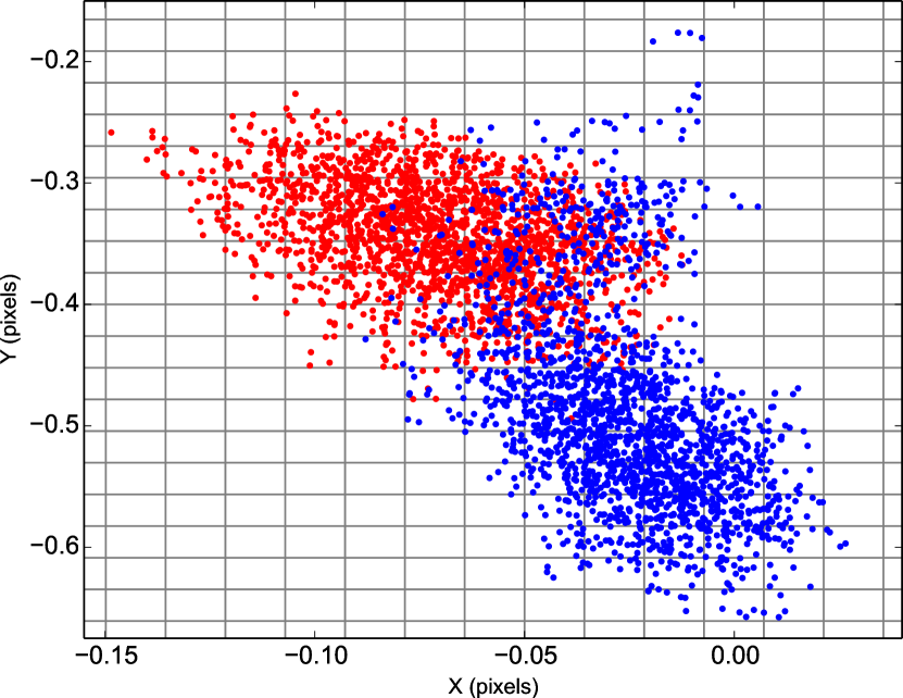
Figure 2.— 3.6 m detector pointing. The blue and red points denote the data point from the first and second AOR, respectively. The coordinate origin denotes the center of the nearest pixel. The grid delimits the BLISS-map bin boundaries.

Note that introducing parameters that relate only to a portion of the data violates an assumption of the Bayesian Information Criterion (BIC) used below; the same violation occurs for the BLISS map (see Appendix A of Stevenson et al. 2012a). We have not found an information criterion that handles such parameters, so we ranked these fits with the others, being aware that BIC penalizes them too harshly. It turned out that the AOR-scaling model made a significan improvement only at 3.6 m; see Section 3.5.7.

To determine the best-fitting parameters, ${\bf x}$, of a model, ${\cal M}$ (Equation 3 in this case), given the data, ${\bf D}$, we maximize the Bayesian posterior probability (probability of the model parameters given the data and modeling framework, Gregory 2005):

$$P({\bf x}|{\bf D},{\cal M})=P({\bf x}|{\cal M})\,P({\bf D}|{\bf x},{\cal M})/P({\bf D}|{\cal M}),$$ (8)

where $P({\bf D}|{\bf x},{\cal M})$ is the usual likelihood of the data given the model and $P({\bf x}|{\cal M})$ is any prior information on the parameters. Assuming Gaussian-distributed priors, maximizing Equation (8) can be turned into a problem of minimization:

$$\min\bigg{\{}\sum_{j}\left(\frac{{\bf x}_{j}-p_{j}}{\sigma_{j}}\right)^{2}+\sum_{i}\left(\frac{{\cal M}_{i}({\bf x})-{\bf D}_{i}}{\sigma_{i}}\right)^{2}\bigg{\}},$$ (9)

with $p_{j}$ a prior estimation (with standard deviation $\sigma_{j}$). The second term in Equation (9) corresponds to $\chi^{2}$. We used the Levenberg-Marquardt minimizer to find ${\bf x}_{j}$ (Levenberg 1944, Marquardt 1963). Next we sampled the parameters’ posterior distribution through a Markov-chain Monte Carlo (MCMC) algorithm to estimate the parameter uncertainties, requiring the Gelman-Rubin statistic (Gelman & Rubin 1992) to be within 1% of unity for each free parameter before declaring convergence.

3.3. Differential Evolution Markov Chain

The MCMC’s performance depends crucially on having good proposal distributions to efficiently explore the parameter space. Previous POET versions used the Metropolis random walk, where new parameter sets are proposed from a multivariate normal distribution. The algorithm’s efficiency was limited by the heuristic tuning of the characteristic jump sizes for each parameter. Too-large values yielded low acceptance rates, while too-small values wasted computational power. Furthermore, highly correlated parameter spaces required additional orthogonalization techniques (Stevenson et al. 2012a) to achieve reasonable acceptance ratios, and even then did not always converge.

We eliminated the need for manual tuning and orthogonalization by implementing the differential-evolution Markov-chain algorithm (DEMC, ter Braak 2006), which automatically adjusts the jumps’ scales and orientations. Consider ${\bf x}_{n}^{i}$ as the set of free parameters of a chain $i$ at iteration $n$. DEMC runs several chains in parallel, drawing the parameter values for the next iteration from the difference between the current parameter states of two other randomly-selected chains, $j$ and $k$:

$${\bf x}_{n+1}^{i}={\bf x}_{n}^{i}+\gamma\left({\bf x}_{n}^{j}-{\bf x}_{n}^{k}\right)+\gamma_{2}{\bf e}_{n}^{i},$$ (10)

where $\gamma$ is a scaling factor of the proposal jump. Following ter Braak (2006), we selected $\gamma=2.38/\sqrt{2d}$ (with $d$ being the number of free parameters) to optimize the acceptance probability ($\gtrsim$25%, Roberts et al. 1997). The last term, $\gamma_{2}{\bf e}$, is a random distribution (of smaller scale than the posterior distribution) that ensures a complete exploration of posterior parameter space. We chose a multivariate normal distribution for e, scaled by the factor $\gamma_{2}$.

As noted by Eastman et al. (2013), each parameter of $\bf e$ requires a specific jump scale. One way to estimate the scales is to calculate the standard deviation of the parameters in a sample chain run. In a second method (similar to that of Eastman et al. 2013), we searched for the limits around the best-fitting value where $\chi^{2}$ increased by 1 along the parameter axes. We varied each parameter separately, keeping the other parameters fixed. Then, we calculated the jump scale from the difference between the upper and lower limits, $({\bf x}^{\rm up}-{\bf x}^{\rm lo})/2$. Both methods yielded similar results in our tests. By testing different values for $\gamma_{2}$, provided that $|\gamma_{2}{\bf e}_{n}^{i}|<|\gamma({\bf x}_{n}^{j}-{\bf x}_{n}^{k})|$, we found that each trial returned identical posterior distributions and acceptance rates, so we arbitrarily set $\gamma_{2}=0.1$.

3.4. Data Set and Model Selection

To determine the best raw light curve (i.e., the selection of centering and photometry method), we minimized the standard deviation of the normalized residuals (SDNR) of the light-curve fit (Campo et al. 2011). This naturally prefers good fits and low-dispersion data.

We use Bayesian hypothesis testing to select the model best supported by the data. Following Raftery (1995), when comparing two models ${\cal M}_{1}$ and ${\cal M}_{2}$ on a data set ${\bf D}$, the posterior odds ($B_{21}$, also known as Bayes factor) indicates the model preferred by the data and the extent to which it is preferred. Assuming that either model is, a priori, equally probable, the posterior odds are given by:

$$B_{21}=\frac{p({\bf D}|{\cal M}_{2})}{p({\bf D}|{\cal M}_{1})}=\frac{p({\cal M}_{2}|{\bf D})}{p({\cal M}_{1}|{\bf D})}\approx\exp\left(-\frac{{\rm BIC}_{2}-{\rm BIC}_{1}}{2}\right).$$ (11)

This is the ${\cal M}_{2}$-to-${\cal M}_{1}$ probability ratio for the models (given the data), with BIC = $\chi^{2}+k\ln{N}$ the Bayesian Information Criterion (Liddle 2007), $k$ the number of free parameters, and $N$ the number of points. Hence, ${\cal M}_{2}$ has a fractional probability of

$$p({\cal M}_{2}|{\bf D})=\frac{1}{1+1/B_{21}}.$$ (12)

We selected the best models as those with the lowest BIC, and assessed the fractional probability of the others (with respect to the best one) using Equation (12).

Recently, Gibson (2014) proposed to marginalize over systematics models rather than use model selection. Although this process is still subjected to the researcher’s choice of systematics models to test, it is a more robust method. Unfortunately, unless we understand the true nature of the systematics to provide a physically motivated model, the modeling process will continue to be an arbitrary procedure. Most of our analyses prefer one of the models over the others. When a second model shows a significant fractional probability ($>0.2$) we reinforce our selection based on additional evidence (is the model physically plausible? or how do the competing models perform in a joint fit?). We are evaluating to include the methods of Gibson (2014) to our pipeline in the future.

3.5. Light-curve Analyses

We initially fit the eclipse light curves individually to determine the best data sets (centering and photometry methods) and systematics models. Then, we determined the definitive parameters from a final joint fit (Section 3.5.7) with shared eclipse parameters. For the eclipse model we fit the midpoint, depth, duration, and ingress time (while keeping the egress time equal to the ingress time). Given the low S/N of the data, the individual events do not constrain all the eclipse parameters well. However, the final joint fit includes enough data to do the job. For the individual fits, we assumed a negligible orbital eccentricity, as indicated by transit and radial-velocity (RV) data, and used the transit duration ($2.497\pm 0.012$ hr) and transit ingress/egress time ($18.51\pm 0.63$ min) from Winn et al. (2007) as priors on the eclipse duration and ingress/egress time. In the final joint-fit experiments, we freed these parameters.

3.5.1 IRAC - 3.6 $\mu$m Eclipse

This observation is divided into two AORs at phase 0.498, causing a systematic flux offset due to IRAC’s intrapixel sensitivity variations. We tested aperture photometry between 1.5 and 3.0 pixels. The eclipse depth is consistent among the apertures, and the minimum SDNR occurs for the 2.5 pixel aperture with Gaussian-fit centering (Figure 3).

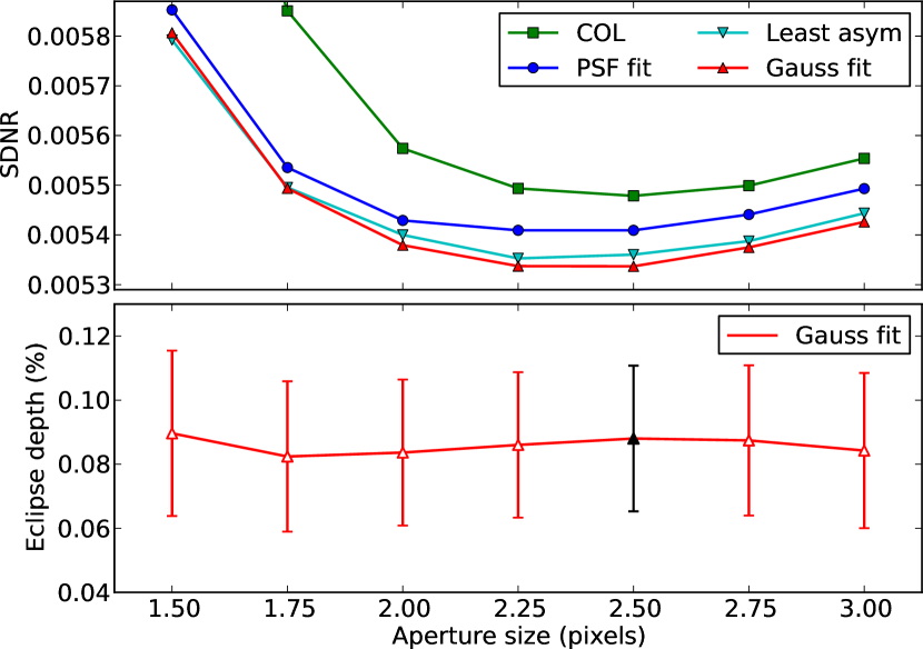
Figure 3.— Top: 3.6 m eclipse light-curve SDNR vs. aperture. The legend indicates the centering method used. All curves used the best ramp model from Table 3. Bottom: Eclipse depth vs. aperture for Gaussian-fit centering, with the best aperture (2.5 pixels) in black.

Table 3 shows the best four model fits at the best aperture; $\Delta$BIC is the BIC difference with respect to the lowest BIC. Given the relatively large uncertainties, more-complex models are not supported, due to the penalty of the additional free parameters. The Bayesian Information Criterion favors the AOR-scaling model (Table 3, last column).

Although the fractional probabilities of the quadratic and exponential ramp models are not negligible, we discard them based on the estimated midpoints, which differ from a circular orbit by 0.008 (twice the ingress/egress duration). It is possible that a non-uniform brightness distribution can induce offsets in the eclipse midpoint (Williams et al. 2006), and these offsets can be wavelength dependent. However, this relative offset can be at most the duration of the ingress/egress. Therefore, disregarding non-uniform brightness offsets, considering the lack of evidence for transit-timing variations and that all other data predict a midpoint consistent with a circular orbit, the 3.6 m offset must be caused by systematic effects. The AOR-scaling model is the only one that yields a midpoint consistent with the rest of the data. Our joint-fit analysis (Section 3.5.7) will provide further support to our model selection.

Table 23.6-m eclipse - ramp model fits

$R(t)\,A({\rm a})$	Ecl. Depth	Midpoint	SDNR	$\Delta$BIC	$p({\cal M}_{2}|D)$
	(%)	(phase)
$A(a)$	0.083(24)	0.501(4)	0.0053763	0.0	$\cdots$
quadramp	0.158(29)	0.492(2)	0.0053712	2.8	0.19
risingexp	0.146(25)	0.492(2)	0.0053715	2.9	0.19
linramp	0.093(23)	0.492(3)	0.0053814	7.4	0.02

We adjusted the BLISS map model following Stevenson et al. (2012a). For a minimum of 4 points per bin, the eclipse depth remained constant for BLISS bin sizes similar to the rms of the frame-to-frame position difference (0.014 and 0.026 pixels in $x$ and $y$, respectively). Figure 4 shows the raw, binned, and systematics-corrected light curves with their best-fitting models.

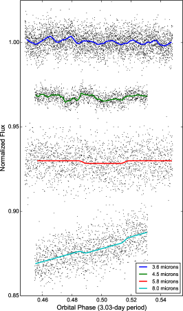
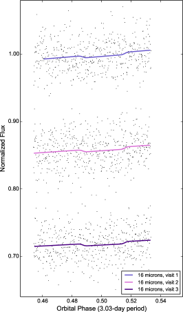
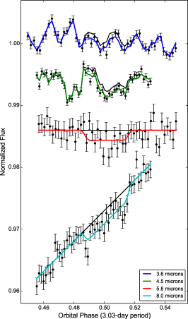
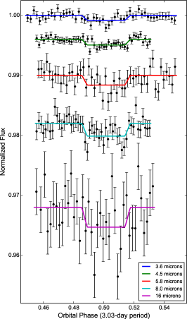
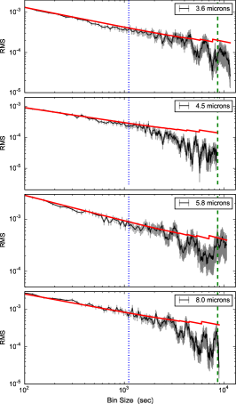
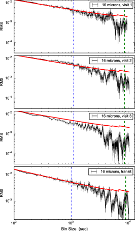
Figure 4.— TrES-1 secondary-eclipse light curves and rms-vs.-bin size plots. Raw light curves are in the top-left and top-center panels. Binned IRAC data are in the top-right panel, and systematics-corrected traces are in the bottom-left panel. The system flux is normalized and the curves are shifted vertically for clarity. The colored solid curves are the best-fit models, while the black solid curves are the best-fit models excluding the eclipse component. The error bars give the 1$\sigma$ uncertainties. The bottom-center and bottom-right panels show the fit residuals’ rms (black curves with 1$\sigma$ uncertainties) vs. bin size. The red curves are the expected rms for Gaussian noise. The blue dotted and green dashed vertical lines mark the ingress/egress time and eclipse duration, respectively.

To estimate the contribution from time-correlated residuals we calculated the time-averaging rms-vs.-bin-size curves (Pont et al. 2006, Winn et al. 2008). This method compares the binned-residuals rms to the uncorrelated-noise (Gaussian noise) rms. An excess rms over the Gaussian rms would indicate a significant contribution from time-correlated residuals. Figure 4 (bottom-center and bottom-right panels) indicates that time-correlated noise is not significant at any time scale, for any of our fits.

3.5.2 IRAC - 4.5 $\mu$m Eclipse

Our analysis of the archival data revealed that the 4.5 m data suffered from multiplexer bleed, or “muxbleed”, indicated by flagged pixels near the target in the mask frames and data-frame headers indicating a muxbleed correction. Muxbleed is an effect observed in the IRAC InSb arrays (3.6 and 4.5 m) wherein a bright star trails in the fast-read direction for a large number of consecutive readouts. Since there are 4 readout channels, the trail appears every 4 pixels, induced by one or more bright pixels (Figure 5).

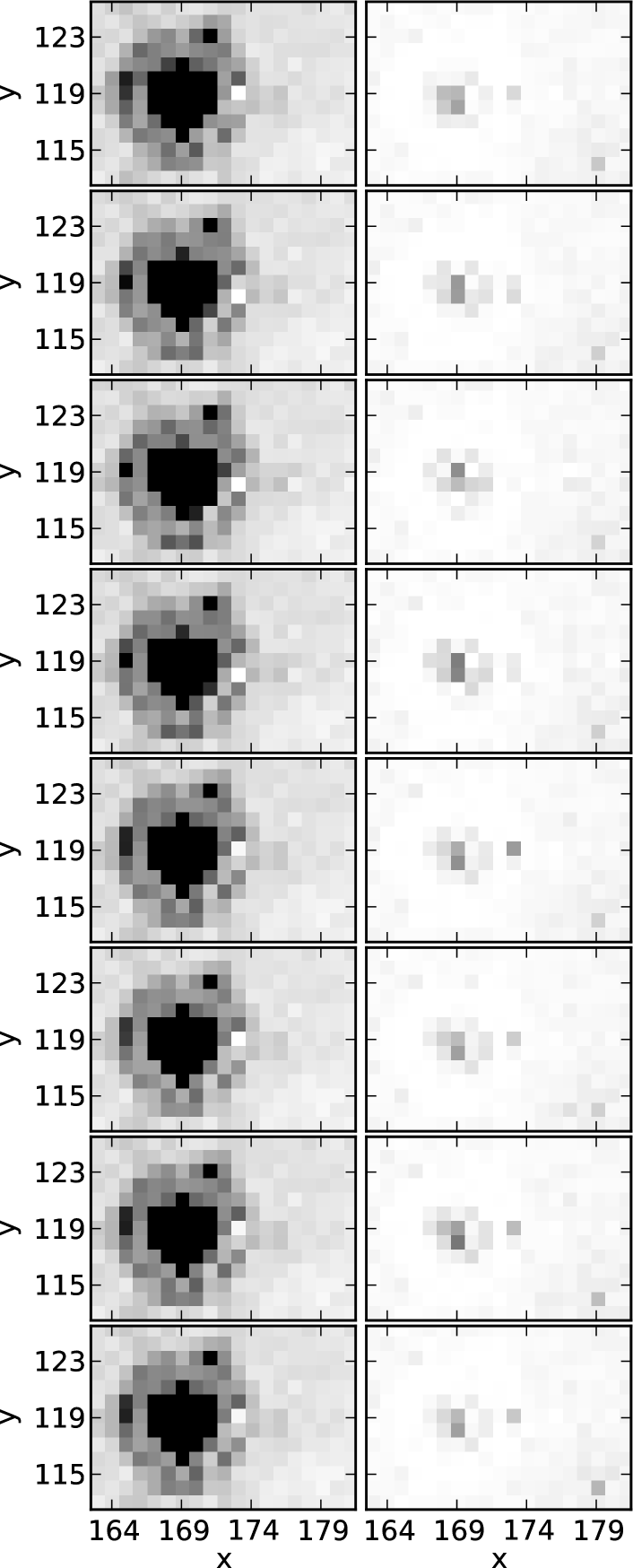
Figure 5.— Left: Per-AOR mean of the Spitzer BCD frames at 4.5 m around TrES-1. Right: Per-AOR rms divided by the square root of the mean BCD frames at 4.5 m. The flux is in electron counts, the color scales range from the 2.5th (white) to the 97.5th (black) percentile of the flux distribution. TrES-1’s center is located near $x=169,y=119$. The miscalculated muxbleed-corrected pixels stand out at 4 and (sometimes) 8 pixels to the right of the target center. The excess in the scaled rms confirms that the muxbleed correction is not linearly scaled with the flux. The pixels around the target center also show high rms values, which might be due to the 0.2 pix motion of the PSF centers.

TrES-1 (whose flux was slightly below the nominal saturation limit at 4.5 m) and a second star that is similarly bright fit the muxbleed description. We noted the same feature in the BCD frames used by Charbonneau et al. (2005, Spitzer pipeline version S10.5.0). Their headers indicated a muxbleed correction as well, but did not clarify whether or not a pixel was corrected.

Since the signal is about $10^{-3}$ times the stellar flux level, every pixel in the aperture is significant and any imperfectly made local correction raises concern (this is why we do not interpolate bad pixels in the aperture, but rather discard frames that have them). Nevertheless, we analyzed the data, ignoring the muxbleed flags, to compare it to the results of Charbonneau et al. (2005). In the atmospheric analysis that follows, we model the planet both with and without this data set.

This light curve is also mainly affected by the intrapixel effect. Since the 4.5 m light curve consisted of 8 AORs, some of which are entirely in- or out-of-eclipse, making the AOR-scale model to overfit the data. We tested apertures between 2.5 and 4.5 pixels, finding the lowest SDNR for the center-of-light centering method at the 3.75-pixel aperture (Figure 6). This alone is surprising, as it may be the first time in our experience that center of light is the best method. In the same manner as for the 3.6 m data, we selected BLISS bin sizes of 0.018 ($x$) and 0.025 ($y$) pixels, for 4 minimum points per bin. A fit with no ramp model minimized BIC (Table 7). Figure 4 shows the data and best-fitting light curves and the rms-vs.-bin size plot.

Table 34.5-m Eclipse - ramp model fits

$R(t)\,A({\rm a})$	Ecl. Depth (%)	SDNR	$\Delta$BIC	$p({\cal M}_{2}|D)$
no-model	0.090(28)	0.0026543	0.0	$\cdots$
linramp	0.091(27)	0.0026531	6.0	0.05
risingexp	0.131(32)	0.0026469	7.1	0.03
quadamp	0.153(39)	0.0026481	8.7	0.01
logramp	0.090(22)	0.0026532	13.3	$1\times 10^{-3}$
$A(a)$	0.140(43)	0.0026474	38.5	$4\times 10^{-9}$

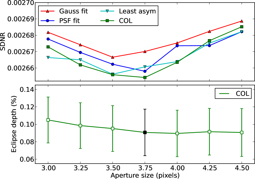
Figure 6.— Top: 4.5 m eclipse light-curve SDNR vs. aperture. The legend indicates the centering method used. All curves used the best ramp model from Table 7. Bottom: Eclipse depth vs. aperture for center-of-light centering, with the best aperture (3.75 pixels) in black.

3.5.3 IRAC - 5.8 $\mu$m Eclipse

These data are not affected by the intrapixel effect. We sampled apertures between 2.25 and 3.5 pixels. Least-asymmetry centering minimized the SDNR at 2.75 pixels, with all apertures returning consistent eclipse depths (Figure 7). The BIC comparison favors a fit without AOR-scale nor ramp models, although, at some apertures the midpoint posterior distributions showed a hint of bi-modality. The eclipse depth, however, remained consistent for all tested models (Table 9). Figure 4 shows the data and best-fitting light curves and rms-vs.-bin size plot.

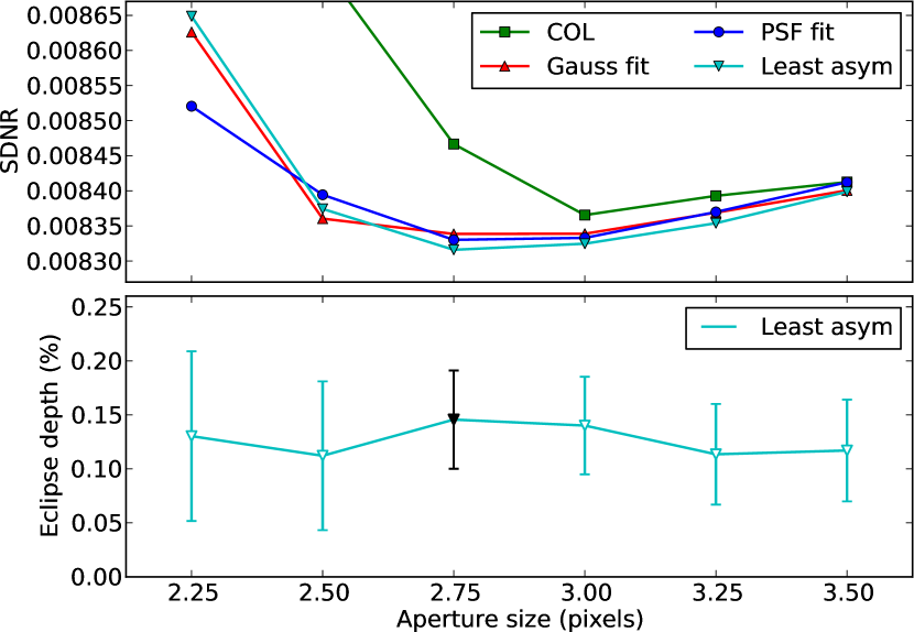
Figure 7.— Top: 5.8 m eclipse light-curve SDNR vs. aperture. The legend indicates the centering method used. All curves used the best ramp model from Table 9. Bottom: Eclipse depth vs. aperture for least-asymmetry centering, with the best aperture (2.75 pixels) in black.

Table 45.8-m Eclipse - ramp model fits

$R(t)\,A({a})$	Ecl. Depth (%)	SDNR	$\Delta$BIC	$p({\cal M}_{2}|D)$
no-model	0.158(44)	0.0083287	0.0	$\cdots$
$A(a)$	0.142(45)	0.0083220	4.4	0.10
linramp	0.154(44)	0.0083281	7.2	0.03
quadramp	0.100(54)	0.0083259	13.0	$2\times 10^{-3}$
risingexp	0.158(44)	0.0083287	14.9	$6\times 10^{-4}$

3.5.4 IRAC - 8.0 $\mu$m Eclipse

This data set had eight AOR blocks. We tested aperture photometry from 1.75 to 3.5 pixels. Again, least-asymmetry centering minimized the SDNR for the 2.75-pixel aperture (Figure 8). We attempted fitting with the per-AOR adjustment $A(a)$, but the seven additional free parameters introduced a large BIC penalty, and the many parameters certainly alias with the eclipse. The linear ramp provided the lowest BIC (Table 11). Figure 4 shows the data and best-fitting light curves and rms-vs.-bin size plot.

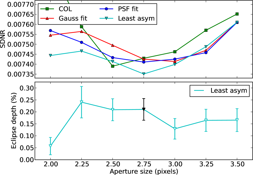
Figure 8.— Top: 8.0 m eclipse light-curve SDNR vs. aperture. The legend indicates the centering method used. All curves used the best ramp model from Table 11. Bottom: Eclipse depth vs. aperture for least-asymmetry centering, with the best aperture (2.75 pixels) in black. This data set had the greatest eclipse-depth variations per aperture.

Table 58.0-m Eclipse - ramp model fits

$R(t)\,A({a})$	Ecl. Depth (%)	SDNR	$\Delta$BIC	$p({\cal M}_{2}|D)$
linramp	0.208(45)	0.0073506	0.0	$\cdots$
quadramp	0.267(62)	0.0073388	3.3	0.16
risingexp	0.278(53)	0.0073389	3.4	0.15
logramp	0.304(45)	0.0073471	7.0	0.03
linramp–$A(a)$	0.759(185)	0.0073112	41.8	$8\times 10^{-10}$

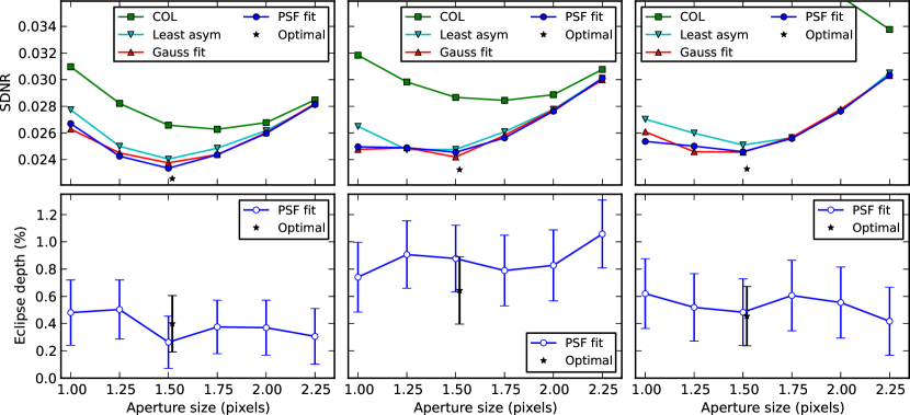
Figure 9.— Top: 16-m eclipse light-curves SDNR vs. aperture (from left to right, the first, second, and third visits, respectively). The legend indicates the centering method used; additionally, the optimal-photometry calculation uses the PSF-fit centering positions but does not involve an aperture. We plotted the optimal-photometry results next to the best-aperture location (for ease of comparison). Each curve used the best ramp model from Tables 13, 15, and 17, respectively. Bottom: Eclipse depth vs. aperture for PSF-fit centering, with the best one (optimal photometry) in black.

3.5.5 IRS - 16-$\mu$m Eclipses

These data come from three consecutive eclipses and present similar systematics. The telescope cycled among four nodding positions every five acquisitions. As a result, each position presented a small flux offset ($\lesssim 2\%$). Since the four nod positions are equally sampled throughout the entire observation, they should each have the same mean level. We corrected the flux offset by dividing each frame’s flux by the nodding-position mean flux and multiplying by the overal mean flux, improving SDNR by $\sim 6\%$. We tested aperture photometry from 1.0 to 5.0 pixels. In all visits the SDNR minimum was at an aperture of 1.5 pixels; however, optimal photometry outperformed aperture photometry (Figure 9). The second visit provided the clearest model determination (Table 13).

Table 616-m eclipse, visit 2 - individual ramp model fits

$R(t)$	Ecl. Depth (%)	SDNR	$\Delta$BIC	$p({\cal M}_{2}|D)$
linramp	0.50(24)	0.0233022	0.0	$\cdots$
no-ramp	0.40(19)	0.0235462	4.1	0.11
quadramp	0.74(28)	0.0232539	5.3	0.06
risingexp	0.68(22)	0.0232595	5.3	0.06

At the beginning of the third visit (40 frames, $\sim$ 28 min), the target position departs from the rest by half a pixel; omitting the first 40 frames did not improve SDNR. The linear ramp model minimized BIC (Table 15). Even though $\Delta$BIC between the linear and the no-ramp models was small, the no-ramp residuals showed a linear trend, thus we are confident on having selected the best model. The eclipse light curve in this visit is consistent with that of the second visit.

Table 716-m eclispe, visit 3 - individual ramp model fits

$R(t)$	Ecl. Depth (%)	SDNR	$\Delta$BIC	$p({\cal M}_{2}|D)$
linramp	0.48(21)	0.0233010	0.0	$\cdots$
no-ramp	0.24(18)	0.0234888	1.1	0.37
quadramp	0.38(22)	0.0233004	5.8	0.05
risingexp	0.48(20)	0.0233011	6.2	0.04

The eclipse of the first visit had the lowest S/N of all. The free parameters in both minimizer and MCMC easily ran out of bounds towards implausible solutions. For this reason we determined the best model in a joint fit combining all three visits. The events shared the eclipse midpoint, duration, depth, and ingress/egress times. We used the best data sets and models from the second and third visits and tested different ramp models for the first visit. With this configuration, the linear ramp model minimized the BIC of the joint fit (Table 17). Here, the target locations in the first two nodding cycles also were shifted with respect to the rest of the frames. Clipping them out improved the SDNR. Figure 4 shows the data and best-fitting light curves and rms-vs.-bin size plot.

Table 816-m eclipse, visit 1 - ramp model fits

$R(t)$	Ecl. Depth (%)	SDNR	$\Delta$BIC	$p({\cal M}_{2}|D)$
tr001bs51	Joint	Joint	Joint	tr001bs51
linramp	0.35(14)	0.0230156	00.00	$\cdots$
quadramp	0.32(14)	0.0230172	07.10	0.03
risingexp	0.36(11)	0.0230152	07.31	0.02
no-ramp	0.33(13)	0.0231502	10.16	$6\times 10^{-3}$

3.5.6 IRS - 16-$\mu$m Transit

To fit this light curve we used the Mandel & Agol (2002) small-planet transit model with a quadratic limb-darkening law. We included priors on the model parameters that were poorly constrained by our data. We adopted $\cos(i)=0.0^{+0.019}_{-0.0}$ and $a/R_{\star}=10.52^{+0.02}_{-0.18}$ from Torres et al. (2012) and the quadratic-limb darkening coefficients $u_{1}=0.284\pm 0.061$ and $u_{2}=0.21\pm 0.12$, which translate into our model parameters as $c_{2}=u_{1}+2u_{2}=-0.7\pm 0.25$ and $c_{4}=-u_{2}=-0.21\pm 0.12$ (with $c_{1}=c_{3}=0$) from Winn et al. (2007). The midpoint and planet-to-star radius ratio completed the list of free parameters for the transit model.

We tested aperture photometry between 1 and 2 pixels, finding the SDNR minimum at 1.5 pixels for the Gaussian-fit centering method (Figure 10). Table 19 shows the ramp-model fitting results. The linear ramp minimized BIC followed by the quadratic ramp with a 0.33 fractional probability; however, the quadratic fit shows an unrealistic upward curvature due to high points at the end of the observation. Figures 11 and 4 show the best fit to the light curve and the rms-vs.-bin size plot, respectively.

Table 916 m Transit - ramp model fits

$R(t)$	$R_{p}/R_{\star}$	SDNR	$\Delta$BIC	$p({\cal M}_{2}|D)$
linramp	0.1314(86)	0.0247755	0.0	$\cdots$
quadramp	0.1069(224)	0.0247118	1.4	0.33
risingexp	0.1314(92)	0.0247757	6.2	0.04
logramp	0.1316(81)	0.0247768	6.3	0.04
no-ramp	0.1306(89)	0.0250938	6.9	0.03

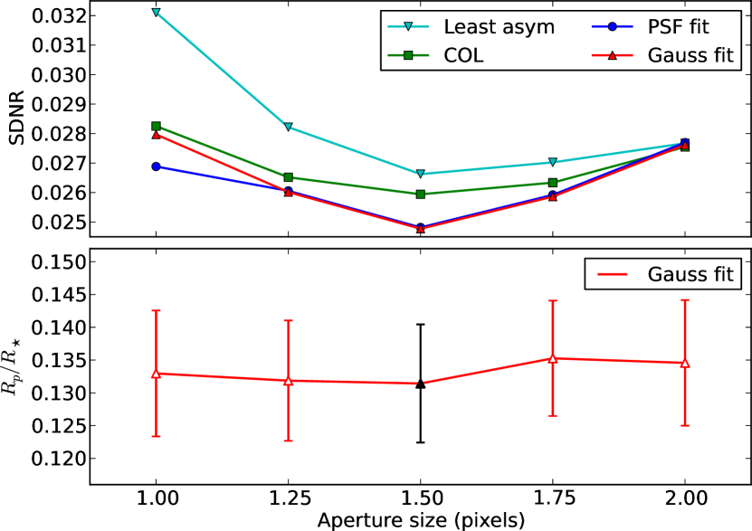
Figure 10.— Top: 16-m transit light-curve SDNR vs. aperture. All curves used the best ramp model from Table 19. Bottom: Planet-to-star radius ratio vs. aperture for least asymmetry centering, with the best aperture (2.75 pixels) in black.

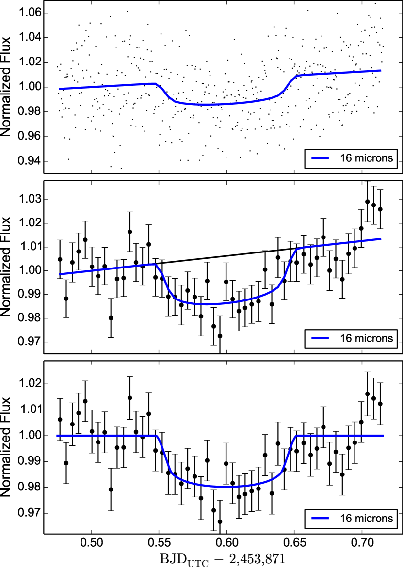
Figure 11.— Raw (top), binned (middle), and systematics-corrected (bottom) normalized TrES-1 transit light curves at 16 m. The colored curves are the best-fit models. The black curve is the best-fit model excluding the transit component. The error bars are $1\sigma$ uncertainties.

3.5.7 Joint-Fit Analysis

We used the information from all eclipse light curves combined to perform a final joint-fit analysis. The simultaneous fit shared a common eclipse duration, eclipse midpoint and eclipse ingress/egress time among all light curves. Additionally, the three IRS eclipses shared the eclipse-depth parameter. We further released the duration prior (which assumed a circular orbit). We also performed experiments related to the 3.6 and 4.5 m datasets.

First, to corroborate our selection of the 3.6 m model, we compared the different 3.6 m models in the joint-fit configuration both with the shared-midpoint constraint and with independently-fit midpoints per waveband (Tables 10 and 11).

Table 103.6 m eclipse models - eclipse-joint fits

$R(t)A(a)$	$\Delta$BIC	3.6 m Ecl.	Midpoint	Duration
	3.6 m	Depth (%)	(phase)	(phase)
Independently-fit midpoints:
$A(a)$	0.0	0.09(2)	$\cdots$	0.032(1)
quadramp	2.3	0.16(2)	$\cdots$	0.032(1)
risingexp	2.9	0.15(2)	$\cdots$	0.032(1)
linramp	6.9	0.10(2)	$\cdots$	0.032(1)
Shared midpoint:
$A(a)$	0.0	0.08(2)	0.5015(6)	0.0328(9)
quadramp	13.3	0.14(3)	0.5013(5)	0.0331(9)
linramp	14.2	0.08(2)	0.5015(6)	0.0328(9)
risingexp	15.0	0.12(2)	0.5013(5)	0.0330(9)

Table 11Midpoint per waveband - eclipse-joint fit

$R(t)A(a)$	3.6 m	4.5 m	5.8 m	8.0 m	16 m
	(phase)	(phase)	(phase)	(phase)	(phase)
$A(a)$	0.500(3)	0.503(1)	0.502(4)	0.501(1)	0.499(3)
quadramp	0.493(2)	0.503(1)	0.502(4)	0.501(1)	0.500(4)
risingexp	0.493(1)	0.503(1)	0.502(4)	0.501(1)	0.500(3)
linramp	0.491(1)	0.503(1)	0.507(4)	0.501(1)	0.499(3)

All wavebands other than 3.6 m agreed with an eclipse midpoint slightly larger than 0.5. When we fit the midpoint separately for each waveband, only the AOR-scale model at 3.6 m agreed with the other bands’ midpoint (note that the 5.8 m data were obtained simultaneously with the 3.6 m data, and should have the same midpoint). The posterior distributions also showed midpoint multimodality between these two solutions (Figure 12). On the other hand, with a shared midpoint, the 3.6 m band assumed the value of the other bands for all models, with no multimodality. All but the AOR-scale model showed time-correlated noise, further supporting it as the best choice.

Second, we investigated the impact of the (potentially corrupted) 4.5 m data set on the joint-fit values. Excluding the 4.5 m event from the joint fit does not significantly alter the midpoint (phase $0.5011~{}\pm~{}0.0006$) nor the duration ($0.0326~{}\pm~{}0.013$). Our final joint fit configuration uses the AOR-scaling model for the 3.6 m band, includes the 4.5 m light curve, and shares the eclipse midpoint (Table B.1).

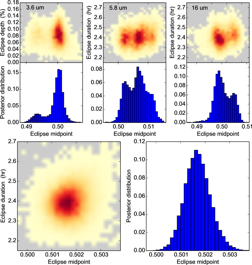
Figure 12.— Eclipse-midpoint pairwise and marginal posteriors. Top: Independently-fit posterior eclipse depth or duration vs. midpoint for (left to right) 3.6, 5.8, and 16.0 m. The multi-modality did not replicate for the eclipse depth (same eclipse depth for each of the posterior modes). Bottom: Eclipse-duration vs. midpoint pairwise (left) and midpoint marginal (right) posterior distributions for the fit with shared midpoint.

3.5.8 4.5 and 8.0 $\mu$m Eclipse Reanalyses

Our current analysis methods differ considerably from those of nearly a decade ago, with better centering, subpixel aperture photometry, BLISS mapping, simultaneous fits across multiple data sets, and evaluation of multiple models using BIC. Furthermore, MCMC techniques were not yet prominent in most exoplanet analyses, among other improvements. Charbonneau et al. (2005) used two field stars (with similar magnitudes to TrES-1) as flux calibrators. They extracted light curves using aperture photometry with an optimal aperture of 4.0 pixels, based on the rms of the calibrators’ flux. At 4.5 m, they decorrelated the flux from the telescope pointing, but gave no details. At 8.0 m, they fit a third-order polynomial to the calibrators to estimate the ramp. Their eclipse model had two free parameters (depth and midpoint), which they fit by mapping $\chi^{2}$ over a phase-space grid. Table 12 compares their eclipse depths with ours, showing a marginal 1$\sigma$ difference at 4.5 m. In both channels our MCMC found larger eclipse-depth uncertainties compared to those of Charbonneau et al. (2005), who calculated them from the $\chi^{2}$ contour in the phase-space grid. The introduction of MCMC techniques and the further use of more efficient algorithms (e.g., differential-evolution MCMC) that converge faster enabled better error estimates. In the past, for example, a highly-correlated posterior prevented the MCMC convergence of some nuisance (systematics) parameters. The non-convergence forced one to fix these parameters to their best-fitting values. In current analyses, however, marginalization over nuisance parameters often leads to larger but more realistic error estimates.

The muxbleed correction was likely less accurately made than required for atmospheric characterization, given the presence of a visible muxbleed trail in the background near the star. We cannot easily assess either the uncertainty or the systematic offset added by the muxbleed and its correction, given, e.g., that the peak pixel flux varies significantly with small image motions. Our stated 4.5 m uncertainty contains no additional adjustment for this unquantified noise source, which makes further use of the 4.5 m eclipse depth difficult. However, our minimizer and the $\chi^{2}$ map of Charbonneau et al. clearly find the eclipse, so the timing and duration appear less affected than the depth. In the analyses below, we include fits both with and without this dataset. The large uncertainty found by MCMC limits the 4.5 m point’s influence in the atmospheric fit.

Table 12Eclipse-depth reanalysis

Eclipse depth (%)	4.5 m	8.0 m
Charbonneau et al. (2005)	0.066(13)	0.225(36)
This work	0.094(24)	0.213(42)

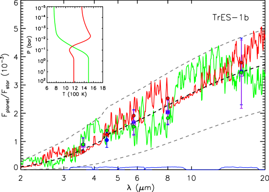
Figure 13.— Left: Dayside atmospheric spectral emission of TrES-1. The blue circles and purple squares with error bars are the measured eclipse depths (including and excluding the 4.5 m data point, respectively). The red and green curves show representative model spectra with and without thermal inversion (see inset), based on the data including the 4.5 m point. Results omitting this point are similar. Both models have a solar abundance atomic composition and are in chemical equilibrium for the corresponding temperature profiles. The red and green circles give the band-integrated (bottom curves) fluxes of the corresponding models, for comparison to data. The dashed lines represent planetary blackbody spectra with $T$ = 800, 1200, and 1500 K. Right: Normalized contribution functions of the models over each Spitzer band (see legend). The dotted and solid lines are for the models with and without thermal inversion, respectively.

4. ORBITAL DYNAMICS

As a preliminary analysis, we derived $e\cos(\omega)$ from the eclipse data alone. Our seven eclipse midpoint times straddle phase 0.5. After subtracting a light-time correction of $2a/c=39$ seconds, where $a$ is the semimajor axis and $c$ is the speed of light, we found an eclipse phase of $0.5015\pm 0.0006$. This implies a marginal non-zero value for $e\cos(\omega)$ of $0.0023\pm 0.0009$ (under the small-eccentricity approximation, Charbonneau et al. 2005).

It is possible that a non-uniform brightness emission from the planet can lead to non-zero measured eccentricity (Williams et al. 2006). For example, a hotspot eastward from the substellar point can simulate a late occultation ingress and egress compared to the uniform-brightness case. However, as pointed out by (de Wit et al. 2012), to constrain the planetary brightness distribution requires a higher photometric precision than what TrES-1 can provide.

Further, using the MCMC routine described by Campo et al. (2011), we fit a Keplerian-orbit model to our secondary-eclipse midpoints simultaneously with 33 radial-velocity (Table B.2) and 84 transit data points (Table B.3). We discarded nine radial-velocity points that were affected by the Rossiter-McLauglin effect. We were able to constrain $e\cos(\omega)$ to $0.0017\pm 0.0003$. Although this 3$\sigma$ result may suggest a non-circular orbit, when combined with the fit to $e\sin(\omega)$ of $-0.033\pm 0.025$, the posterior distribution for the eccentricity only indicates a marginally eccentric orbit with $e=0.033^{+0.015}_{-0.031}$. Table 13 summarizes our orbital MCMC results.

Table 13 MCMC Eccentric Orbital Model

Parameter	Best fitting value
$e\sin\omega$	$-0.033$ $\pm$ 0.025
$e\cos\omega$	0.0017 $\pm$ 0.0003
$e$	0.033 ${}^{+0.015}_{-0.031}$
$\omega$ (°)	273 ${}^{+1.4}_{-2.8}$
Orbital period (days)	3.0300699 $\pm$ $1\times 10^{-7}$
Transit time, $T_{0}$ (MJD)	3186.80692 $\pm$ 0.00005
RV semiamplitude, $K$ (m s-1)	115.5 $\pm$ 3.6
system RV, $\gamma$ (m s-1)	$-3.9$ $\pm$ 1.3
Reduced $\chi^{2}$	6.2

5. ATMOSPHERE

We modeled the day-side emergent spectrum of TrES-1 with the retrieval method of Madhusudhan & Seager (2009) to constrain the atmospheric properties of the planet. The code solves the plane-parallel, line-by-line, radiative transfer equations subjected to hydrostatic equilibrium, local thermodynamic equilibrium, and global energy balance. The code includes the main sources of opacity for hot Jupiters: molecular absorption from H₂O, CH₄, CO, and CO₂ (Freedman et al. 2008, Freedman, personal communication 2009), and H₂-H₂ collision induced absorption (Borysow 2002). We assumed a Kurucz stellar spectral model (Castelli & Kurucz 2004).

The model’s atmospheric temperature profile and molecular abundances of H₂O, CO, CH₄, and CO₂ are free parameters, with the abundance parameters scaling initial profiles that are in thermochemical equilibrium. The output spectrum is integrated over the Spitzer bands and compared to the observed eclipse depths by means of $\chi^{2}$. An MCMC module supplies millions of parameter sets to the radiative transfer code to explore the phase space (Madhusudhan & Seager 2010, 2011).

Even though the features of each molecule are specific to certain wavelengths (Madhusudhan & Seager 2010), our independent observations (4 or 5) are less than the number of free parameters (10), and thus the model fitting is a degenerate problem. Thus, we stress that our goal is not to reach a unique solution, but to discard and/or constrain regions of the parameter phase space given the observations, as has been done in the past (e.g., Barman et al. 2005, Burrows et al. 2007, Knutson et al. 2008, Madhusudhan & Seager 2009, Stevenson et al. 2010, Madhusudhan et al. 2011).

Figure 13 shows the TrES-1 data points and model spectra of its day-side emission. An isothermal model can fit the observations reasonably well, as shown by the black dashed line (blackbody spectrum with a temperature of 1200 K). However, given the low S/N of the data, we cannot rule out non-inverted nor strong thermal-inversion models (with solar abundance composition in chemical equilibrium), as both can fit the data equally well (green and red models). Generally speaking, the data allow for efficient day-night heat redistribution; the models shown have maximum possible heat redistributions of 60% (non-inversion model) and 40% (inversion model).

As shown in Fig. 13, the data sets with and without the 4.5 m point are nearly identical. Combined with the large error bars (especially at 16 m), there is no significant difference between the atmospheric model results of the two cases. Both CO and CO₂ are dominant absorbers at 4.5 m. Combined with the 16-m detection, which is mainly sensitive to CO₂, the data could constrain the abundances of CO and CO₂. Unfortunately, the error bar on the 16 m band is too large to derive any meaningful constraint.

6. CONCLUSIONS

We have analyzed all the Spitzer archival data for TrES-1, comprising eclipses in five different bands (IRAC and IRS blue peak-up) and one IRS transit. There has been tremendous improvement in data-analysis techniques for Spitzer, and exoplanet light curves in general, since Charbonneau et al. (2005), one of the first two reported exoplanet secondary eclipses. A careful look at the 4.5 m data frames revealed pixels affected by muxbleed that, although corrected by the Spitzer pipeline, still showed a clear offset output level. Unable to know the effect on the eclipse depth and uncertainty, we conducted subsequent modeling both with and without the 4.5 m point. The already-large uncertainty resulted in similar conclusions either way. Without adjusting our point for either the systematic or random effects of the muxbleed correction, the depth and uncertainty at 4.5 m are both substantially larger than the original analysis. However, at 8.0 m (which does not have similar problems) the eclipse depths are consistent, with our MCMC giving a larger uncertainty.

Our measured eclipse depths from our joint light-curve fitting (with and without the 4.5 m point) are consistent with a nearly-isothermal atmospheric dayside emission at $\sim 1200$ K. This is consistent with the expected equilibrium temperature of 1150 K (assuming zero albedo and efficient energy redistribution). Furthermore, neither inverted nor non-inverted atmospheric models can be ruled out, given the low S/N of the data. Our transit analysis unfortunately does not improve the estimate of the planet-to-star radius ratio ($R_{p}/R_{\star}=0.119{\pm}0.009$). Our comprehensive orbital analysis of the available eclipse, transit, and radial-velocity data indicates an eccentricity of $e=0.034^{+0.014}_{-0.032}$, consistent with a circular orbit at the 1$\sigma$-level. Longitudinal variations in the planet’s emission can induce time offsets in eclipse light curves, and could mimic non-zero eccentricities (e.g., Williams et al. 2006, de Wit et al. 2012). However, the S/N required to lay such constraints are much higher than that of the TrES-1 eclipse data.

We also described the latest improvements of our POET pipeline. Optimal photometry provides an alternative to aperture photometry. We first applied optimal photometry in Stevenson et al. (2010), but describe it in more detail here. Furthermore, the Differential-Evolution Markov-chain algorithm poses an advantage over a Metropolis Random Walk MCMC, since it automatically tunes the scale and orientation of the proposal distribution jumps. This dramatically increases the algorithm’s efficiency, converging nearly ten times faster. We also now avoid the need to orthogonalize highly correlated posterior distributions.

Appendix A Joint Best Fit

Table B.1 summarizes the model setting and results of the light-curve joint fit. The midpoint phase parameter was shared among the IRS eclipse observations.

Table B.2 lists the aggregate TrES1 radial-velocity measurements.

Table B.3 lists the aggregate TrES1 transit-midpoint measurements.

Appendix B Light-curves Data Sets

All the light-curve data sets are available in flexible Image Transport System (FITS) format in a tar.gz package in the electronic edition.

Table B.1 Best-Fit Eclipse Light-Curve Parameters

Parameter	tr001bs11	tr001bs21	tr001bs31	tr001bs41	tr001bs51	tr001bs52	tr001bs53	tr001bp51
Centering algorithm	Gauss fit	Center of Light	Least Asymmetry	Least Asymmetry	PSF fit	PSF fit	PSF fit	Gauss fit
Mean $x$ position (pix)	119.95	169.02	113.74	167.92	$\cdots$	$\cdots$	$\cdots$	$\cdots$
Mean $y$ position (pix)	82.58	118.63	83.29	117.62	$\cdots$	$\cdots$	$\cdots$	$\cdots$
$x$-position consistency (pix)	0.014	0.019	0.021	0.019	0.038	0.036	0.040	0.045
$y$-position consistency (pix)	0.026	0.025	0.024	0.030	0.044	0.036	0.043	0.037
Optimal/Aperture photometry size (pix)	2.50	3.75	2.75	2.75	optimal	optimal	optimal	1.5
Inner sky annulus (pix)	7.0	7.0	7.0	7.0	5.0	5.0	5.0	5.0
Outer sky annulus (pix)	15.0	15.0	15.0	15.0	10.0	10.0	10.0	10.0
BLISS mapping	Yes	Yes	No	No	No	No	No	No
Minimum Points Per Bin	4	4	$\cdots$	$\cdots$	$\cdots$	$\cdots$	$\cdots$	$\cdots$
System flux $F_{s}$ (Jy)	33191.4(5.9)	21787.0(2.3)	14184.5(3.3)	8440.7(2.3)	1792.3(2.1)	1797.2(2.3)	1796.6(2.3)	857(1.8)
Eclipse depth (%)	0.083(24)	0.094(24)	0.162(42)	0.213(42)	0.33(12)	0.33(12)	0.33(12)	$\cdots$
Brightness temperature (K)	1270(110)	1126(90)	1205(130)	1190(130)	1270(310)	1270(310)	1270(310)	$\cdots$
Eclipse midpoint (orbital phase)	0.5015(5)	0.5015(5)	0.5015(5)	0.5015(5)	0.5015(5)	0.5015(5)	0.5015(5)	$\cdots$
Eclipse/Transit midpoint (MJDUTC)	3630.7152(16)	3309.5283(16)	3630.7152(16)	3309.5283(16)	3873.1204(16)	3876.1504(16)	3879.1805(16)	$3871.5998(38)$
Eclipse/Transit midpoint (MJDTDB)	3630.7159(16)	3309.5290(16)	3630.7159(16)	3309.5290(16)	3873.1211(16)	3876.1512(16)	3879.1812(16)	$3871.6005(38)$
Eclipse/Transit duration ($t_{\rm 4-1}$, hrs)	2.39(7)	2.39(7)	2.39(7)	2.39(7)	2.39(7)	2.39(7)	2.39(7)	2.496(33)
Ingress/egress time ($t_{\rm 2-1}$, hrs)	0.31(1)	0.31(1)	0.31(1)	0.31(1)	0.31(1)	0.31(1)	0.31(1)	0.28(2)
$R_{p}/R_{\star}$	$\cdots$	$\cdots$	$\cdots$	$\cdots$	$\cdots$	$\cdots$	$\cdots$	0.1295(95)
$\cos(i)$	$\cdots$	$\cdots$	$\cdots$	$\cdots$	$\cdots$	$\cdots$	$\cdots$	$0.0^{+0.000008}_{-0.0}$
$a/R_{\star}$	$\cdots$	$\cdots$	$\cdots$	$\cdots$	$\cdots$	$\cdots$	$\cdots$	$10.494^{+0.092}_{-0.135}$
Limb darkening coefficient, $c2$	$\cdots$	$\cdots$	$\cdots$	$\cdots$	$\cdots$	$\cdots$	$\cdots$	0.75(22)
Limb darkening coefficient, $c2$	$\cdots$	$\cdots$	$\cdots$	$\cdots$	$\cdots$	$\cdots$	$\cdots$	$-0.19(11)$
Ramp equation ($R(t)$)	$A(a)$	None	None	linramp	linramp	linramp	linramp	linramp
Ramp, linear term ($r_{1}$)	$\cdots$	$\cdots$	$\cdots$	0.2455(82)	0.182(49)	0.151(42)	0.118(47)	0.063(17)
AOR scaling factor ($A(a_{2})$)	1.00234(33)	$\cdots$	$\cdots$	$\cdots$	$\cdots$	$\cdots$	$\cdots$	$\cdots$
Number of free parameters	6	5	5	6	6	6	6	8
Total number of frames	3904	1518	1952	1518	500	500	500	500
Frames used	3827	1407	1763	1482	460	500	500	492
Rejected frames (%)	1.97	7.31	9.68	2.37	8.0	0.0	0.0	1.6
BIC value	10103.0	10103.0	10103.0	10103.0	10103.0	10103.0	10103.0	533.4
SDNR	0.0053766	0.0026650	0.0083273	0.0074324	0.0223287	0.0233603	0.0233306	0.0248263
Uncertainty scaling factor	0.946	1.065	1.186	0.962	0.543	0.574	0.590	0.489
Photon-limited S/N (%)	99.34	89.67	74.04	63.01	8.34	7.98	7.99	10.7

Table B.2Tres-1 Radial-Velocity Data

Date	RV		Reference
BJD(TDB) $-$ 2450000.0	(m s-1)
3191.77001	$60.4$ $\pm$	12.8	1
3192.01201	$115.1$ $\pm$	8.3	1
3206.89101	$87.1$ $\pm$	16.0	1
3207.92601	$15.8$ $\pm$	10.4	1
3208.73001	$-113.3$ $\pm$	15.0	1
3208.91701	$-98.1$ $\pm$	19.8	1
3209.01801	$-118.4$ $\pm$	15.3	1
3209.73101	$49.8$ $\pm$	15.7	1
3237.97926	$68.32$ $\pm$	3.66	2
3238.83934	$-102.23$ $\pm$	3.27	2
3239.77361	$-24.53$ $\pm$	3.25	2
3239.88499	$10.00$ $\pm$	3.11	2
3240.97686	$70.68$ $\pm$	3.73	2
3907.87017	$18.7$ $\pm$	14.0	3
3907.88138	$30.5$ $\pm$	12.5	3
3907.89261	$54.6$ $\pm$	12.0	3
3907.90383	$24.3$ $\pm$	10.4	3
3907.91505a	$26.4$ $\pm$	11.4	3
3907.92627a	$30.4$ $\pm$	10.9	3
3907.93749a	$22.4$ $\pm$	14.3	3
3907.94872a	$2.9$ $\pm$	11.0	3
3907.95995a	$-7.1$ $\pm$	12.1	3
3907.97118a	$-22.3$ $\pm$	13.3	3
3907.98240a	$-40.5$ $\pm$	13.3	3
3907.99363a	$-39.2$ $\pm$	13.0	3
3908.00487a	$-9.8$ $\pm$	12.2	3
3908.01609a	$-30.5$ $\pm$	13.8	3
3908.02731	$-17.7$ $\pm$	13.6	3
3908.03853	$-24.7$ $\pm$	12.2	3
3908.04977	$-27.5$ $\pm$	11.1	3
3908.06099	$-38.2$ $\pm$	13.3	3
3908.07222	$-23.7$ $\pm$	11.2	3
3908.08344	$-23.0$ $\pm$	9.6	3
a Discarded due to Rossiter-McLaughlin effect.
References: (1) Alonso et al. 2004;
(2) Laughlin et al. 2005; (3) Narita et al. 2007.

Table B.3 TrES-1 Transit Midpoint data

Midtransit date	Error	Source
BJD(TDB) $-$ 2450000.0
6253.23986	0.00105	ETD: Sokov E. N.
6198.69642	0.00119	ETD: Roomian P.
6198.69600	0.00056	ETD: Shadic S.
6177.47937	0.00099	ETD: Emering F.
6168.39577	0.00042	ETD: Mravik J., Grnja J.
6107.79376	0.00032	ETD: Shadic S.
6074.46334	0.00117	ETD: Bachschmidt M.
6074.46253	0.00112	ETD: Emering F.
6071.43377	0.00055	ETD: Carreño
6071.43165	0.00072	ETD: Gaitan J.
6071.43099	0.0007	ETD: Horta F. G.
5886.59953	0.00048	ETD: Shadic S.
5801.75506	0.0004	ETD: Shadic S.
5798.73056	0.00049	ETD: Shadic S.
5795.69991	0.00053	ETD: Walter B., Strickland W., Soriano R.
5795.69903	0.00064	ETD: Walter B., Strickland W., Soriano R.
5795.69797	0.00055	ETD: Walter B., Strickland W., Soriano R.
5777.51807	0.00056	ETD: Centenera F.
5768.42617	0.00042	ETD: V. Krushevska, Yu. Kuznietsova, M. Andreev
5765.39585	0.0004	ETD: V. Krushevska, Yu. Kuznietsova, M. Andreev
5762.36407	0.00037	ETD: V. Krushevska, Yu. Kuznietsova, M. Andreev
5759.33530	0.00049	ETD: V. Krushevska, Yu. Kuznietsova, M. Andreev
5707.81338	0.00093	ETD: Marlowe H., Makely N., Hutcheson M., DePree C.
5680.55402	0.00064	ETD: Sergison D.
5671.46700	0.00114	ETD: Kučáková H.
5671.46384	0.00088	ETD: Vrašták M.
5671.46382	0.0009	ETD: Brát L.
5371.48766	0.00074	ETD: Mihelčič M.
5304.82572	0.00084	ETD: Shadick S.
5095.75034	0.00075	ETD: Rozema G.
5089.69043	0.00109	ETD: Vander Haagen G.
5068.48006	0.00062	ETD: Trnka J.
5062.42088	0.00053	ETD: Sauer T.
5062.42078	0.00046	ETD: Trnka J., Klos M.
5062.42012	0.00046	ETD: Dřevěný R., Kalisch T.
5062.41959	0.0006	ETD: Brát L.
5062.41797	0.00102	ETD: Kučáková H., Speil J.
4998.79649	0.0016	ETD: Garlitz
4971.51779	0.001	ETD: Gregorio
4968.48904	0.00192	ETD: Přibík V.
4968.48811	0.00053	ETD: Trnka J.
4968.48753	0.00028	ETD: Andreev M., Kuznietsova Y., Krushevska V.
4671.54149	0.0021	ETD: Mendez
4662.44989	0.001	ETD: Forne
4383.68459	0.0019	ETD: Sheridan
4380.65579	0.0014	ETD: Sheridan
4362.47423	0.0002	Hrudková et al. (2009)
4359.44430	0.00015	Hrudková et al. (2009)
4356.41416	0.0001	Hrudková et al. (2009)
4356.41324	0.00096	ETD: Andreev M., Kuznietsova Y., Krushevska V.
4350.35296	0.00036	ETD: Andreev M., Kuznietsova Y., Krushevska V.
4347.32322	0.00028	ETD: Andreev M., Kuznietsova Y., Krushevska V.
3907.96406	0.00034	Narita et al. (2007)
3901.90372	0.00019	Winn et al. (2007)
3901.90371	0.0016	Narita et al. (2007)
3898.87342	0.00014	Narita et al. (2007)
Continued on next page

Table A.3TrES-1 Transit Midpoint Data – Continued from previous page

Midtransit date	Error	Source
BJD(TDB) $-$ 2450000.0
3898.87341	0.00014	Winn et al. (2007)
3898.87336	0.00008	Winn et al. (2007)
3895.84298	0.00015	Narita et al. (2007)
3895.84297	0.00018	Winn et al. (2007)
3856.45180	0.0005	ETD: Hentunen
3650.40752	0.00045	ETD: NYX
3550.41568	0.0003	ETD: NYX
3547.38470	0.0012	ETD: NYX
3256.49887	0.00044	ETD: Ohlert J.
3253.46852	0.00057	ETD: Pejcha
3253.46812	0.00038	ETD: Ohlert J.
3247.40751	0.0004	Charbonneau et al. (2005)
3189.83541	0.0019	Charbonneau et al. (2005)
3186.80626	0.00054	Alonso et al. (2004)
3186.80611	0.0003	Charbonneau et al. (2005)
3183.77521	0.0005	Charbonneau et al. (2005)
3174.68641	0.0004	Charbonneau et al. (2005)
2868.65031	0.0022	Charbonneau et al. (2005)
2856.52861	0.0015	Charbonneau et al. (2005)
2847.43631	0.0015	Charbonneau et al. (2005)
2850.47091	0.0016	Charbonneau et al. (2005)
3171.65231	0.0019	Charbonneau et al. (2005)
3192.86941	0.0015	Charbonneau et al. (2005)
3180.75291	0.0010	Charbonneau et al. (2005)
4356.41492	0.00010	Hrudková et al. (2009)
4359.44506	0.00015	Hrudková et al. (2009)
4362.47499	0.00020	Hrudková et al. (2009)

References

- Adams et al. (2013) Adams, E. R., Dupree, A. K., Kulesa, C., & McCarthy, D. 2013, AJ, 146, 9, ADS, 1305.6548
- Alonso et al. (2004) Alonso, R. et al. 2004, ApJ, 613, L153, ADS, arXiv:astro-ph/0408421
- Barman et al. (2005) Barman, T. S., Hauschildt, P. H., & Allard, F. 2005, ApJ, 632, 1132, ADS, arXiv:astro-ph/0507136
- Blecic et al. (2013) Blecic, J. et al. 2013, ApJ, 779, 5, ADS, 1111.2363
- Borysow (2002) Borysow, A. 2002, A&A, 390, 779, ADS
- Burrows et al. (2007) Burrows, A., Hubeny, I., Budaj, J., Knutson, H. A., & Charbonneau, D. 2007, ApJ, 668, L171, ADS, 0709.3980
- Butler et al. (2006) Butler, R. P. et al. 2006, ApJ, 646, 505, ADS, arXiv:astro-ph/0607493
- Campo et al. (2011) Campo, C. J. et al. 2011, ApJ, 727, 125, ADS, arXiv:1003.2763
- Castelli & Kurucz (2004) Castelli, F., & Kurucz, R. L. 2004, ArXiv Astrophysics e-prints, ADS, arXiv:astro-ph/0405087
- Charbonneau et al. (2005) Charbonneau, D. et al. 2005, ApJ, 626, 523, ADS, arXiv:astro-ph/0503457
- Charbonneau et al. (2007) Charbonneau, D., Brown, T. M., Burrows, A., & Laughlin, G. 2007, Protostars and Planets V, 701, ADS, arXiv:astro-ph/0603376
- Cubillos et al. (2013) Cubillos, P. et al. 2013, ApJ, 768, 42, ADS, 1303.5468
- de Wit et al. (2012) de Wit, J., Gillon, M., Demory, B.-O., & Seager, S. 2012, A&A, 548, A128, ADS, 1202.3829
- Deming et al. (2005) Deming, D., Seager, S., Richardson, L. J., & Harrington, J. 2005, Nature, 434, 740, ADS, arXiv:astro-ph/0503554
- Eastman et al. (2013) Eastman, J., Gaudi, B. S., & Agol, E. 2013, PASP, 125, 83, ADS, 1206.5798
- Fazio et al. (2004) Fazio, G. G. et al. 2004, ApJS, 154, 10, ADS
- Freedman et al. (2008) Freedman, R. S., Marley, M. S., & Lodders, K. 2008, ApJS, 174, 504, ADS, 0706.2374
- Gelman & Rubin (1992) Gelman, A., & Rubin, D. B. 1992, Statistical Science, 7, 457
- Gibson (2014) Gibson, N. P. 2014, MNRAS, 445, 3401, ADS, 1409.5668
- Gregory (2005) Gregory, P. 2005, Bayesian Logical Data Analysis for the Physical Sciences (New York, NY, USA: Cambridge University Press), ISBN: 052184150X
- Harrington & French (2010) Harrington, J., & French, R. G. 2010, ApJ, 716, 398, ADS, 1005.3569
- Harrington et al. (2007) Harrington, J., Luszcz, S., Seager, S., Deming, D., & Richardson, L. J. 2007, Nature, 447, 691, ADS
- Horne (1986) Horne, K. 1986, PASP, 98, 609, ADS
- Hrudková et al. (2009) Hrudková, M., Skillen, I., Benn, C., Pollacco, D., Gibson, N., Joshi, Y., Harmanec, P., & Tulloch, S. 2009, in IAU Symposium, Vol. 253, IAU Symposium, ed. F. Pont, D. Sasselov, & M. J. Holman, 446–449, 0807.1000, ADS
- Knutson et al. (2008) Knutson, H. A., Charbonneau, D., Allen, L. E., Burrows, A., & Megeath, S. T. 2008, ApJ, 673, 526, ADS, arXiv:0709.3984
- Knutson et al. (2007) Knutson, H. A., Charbonneau, D., Deming, D., & Richardson, L. J. 2007, PASP, 119, 616, ADS, 0705.4288
- Knutson et al. (2011) Knutson, H. A. et al. 2011, ApJ, 735, 27, ADS, 1104.2901
- Laughlin et al. (2005) Laughlin, G., Wolf, A., Vanmunster, T., Bodenheimer, P., Fischer, D., Marcy, G., Butler, P., & Vogt, S. 2005, ApJ, 621, 1072, ADS
- Levenberg (1944) Levenberg, K. 1944, Quart. Applied Math., 2, 164
- Liddle (2007) Liddle, A. R. 2007, MNRAS, 377, L74, ADS, arXiv:astro-ph/0701113
- Madhusudhan et al. (2011) Madhusudhan, N. et al. 2011, Nature, 469, 64, ADS, arXiv:1012.1603
- Madhusudhan & Seager (2009) Madhusudhan, N., & Seager, S. 2009, ApJ, 707, 24, ADS, 0910.1347
- Madhusudhan & Seager (2010) —. 2010, ApJ, 725, 261, ADS, arXiv:1010.4585
- Madhusudhan & Seager (2011) —. 2011, ApJ, 729, 41, ADS, 1004.5121
- Mandel & Agol (2002) Mandel, K., & Agol, E. 2002, ApJ, 580, L171, ADS, arXiv:astro-ph/0210099
- Marquardt (1963) Marquardt, D. W. 1963, SIAM Journal on Applied Mathematics, 11, 431
- Narita et al. (2007) Narita, N. et al. 2007, PASJ, 59, 763, ADS, arXiv:astro-ph/0702707
- Nymeyer et al. (2011) Nymeyer, S. et al. 2011, ApJ, 742, 35, ADS, 1005.1017
- Pont et al. (2006) Pont, F., Zucker, S., & Queloz, D. 2006, MNRAS, 373, 231, ADS, arXiv:astro-ph/0608597
- Rabus et al. (2009) Rabus, M., Deeg, H. J., Alonso, R., Belmonte, J. A., & Almenara, J. M. 2009, A&A, 508, 1011, ADS, 0909.1564
- Raetz et al. (2009) Raetz, S. et al. 2009, Astronomische Nachrichten, 330, 475, ADS, 0905.1833
- Raftery (1995) Raftery, A. E. 1995, Sociological Mehodology, 25, 111
- Reach et al. (2005) Reach, W. T. et al. 2005, PASP, 117, 978, ADS, astro-ph/0507139
- Roberts et al. (1997) Roberts, G., Gelman, A., & Gilks, W. 1997, Annals of Applied Probability, 7, 110
- Sada et al. (2012) Sada, P. V. et al. 2012, PASP, 124, 212, ADS, 1202.2799
- Santos et al. (2006a) Santos, N. C. et al. 2006a, A&A, 458, 997, ADS, arXiv:astro-ph/0606758
- Santos et al. (2006b) —. 2006b, A&A, 450, 825, ADS, arXiv:astro-ph/0601024
- Seager & Deming (2010) Seager, S., & Deming, D. 2010, ARA&A, 48, 631, ADS, 1005.4037
- Southworth (2008) Southworth, J. 2008, MNRAS, 386, 1644, ADS, 0802.3764
- Southworth (2009) —. 2009, MNRAS, 394, 272, ADS, 0811.3277
- Sozzetti et al. (2006) Sozzetti, A., Yong, D., Carney, B. W., Laird, J. B., Latham, D. W., & Torres, G. 2006, AJ, 131, 2274, ADS, arXiv:astro-ph/0512510
- Steffen & Agol (2005) Steffen, J. H., & Agol, E. 2005, MNRAS, 364, L96, ADS, arXiv:astro-ph/0509656
- Stevenson et al. (2012a) Stevenson, K. B. et al. 2012a, ApJ, 754, 136, ADS, 1108.2057
- Stevenson et al. (2012b) —. 2012b, ApJ, 755, 9, ADS, 1207.4245
- Stevenson et al. (2010) Stevenson, K. B. et al. 2010, Nature, 464, 1161, ADS, arXiv:1010.4591
- ter Braak (2006) ter Braak, C. 2006, Statistics and Computing, 16, 239, 10.1007/s11222-006-8769-1
- Torres et al. (2012) Torres, G., Fischer, D. A., Sozzetti, A., Buchhave, L. A., Winn, J. N., Holman, M. J., & Carter, J. A. 2012, ApJ, 757, 161, ADS, 1208.1268
- Torres et al. (2008) Torres, G., Winn, J. N., & Holman, M. J. 2008, ApJ, 677, 1324, ADS, 0801.1841
- Vaňko et al. (2009) Vaňko, M. et al. 2009, in IAU Symposium, Vol. 253, IAU Symposium, ed. F. Pont, D. Sasselov, & M. J. Holman, 440–442, 0901.0625, ADS
- Williams et al. (2006) Williams, P. K. G., Charbonneau, D., Cooper, C. S., Showman, A. P., & Fortney, J. J. 2006, ApJ, 649, 1020, ADS, astro-ph/0601092
- Winn et al. (2007) Winn, J. N., Holman, M. J., & Roussanova, A. 2007, ApJ, 657, 1098, ADS, arXiv:astro-ph/0611404
- Winn et al. (2008) Winn, J. N. et al. 2008, ApJ, 683, 1076, ADS, arXiv:0804.4475