Geometric Adaptive Tracking Control of a Quadrotor UAV on $\mathsf{SE(3)}$ for Agile Maneuvers

Abstract

This paper presents nonlinear tracking control systems for a quadrotor unmanned aerial vehicle under the influence of uncertainties. Assuming that there exist unstructured disturbances in the translational dynamics and the attitude dynamics, a geometric nonlinear adaptive controller is developed directly on the special Euclidean group. In particular, a new form of an adaptive control term is proposed to guarantee stability while compensating the effects of uncertainties in quadrotor dynamics. A rigorous mathematical stability proof is given. The desirable features are illustrated by numerical example and experimental results of aggressive maneuvers.

$\vec{e}_{i}\in\mathbb{R}^{3}$ Inertial frame $\vec{b}_{i}\in\mathbb{R}^{3}$ Body-fixed frame $m\in\mathbb{R}$ Mass of the quadrotor $J\in\mathbb{R}^{3\times 3}$ Inertia matrix of the quadrotor $R\in\mathbb{R}^{3\times 3}$ Rotation matrix(body-fixed to inertial frame) $\Omega\in\mathbb{R}^{3}$ Angular velocity with respect to body fixed frame $x\in\mathbb{R}^{3}$ Quadrotor position $v\in\mathbb{R}^{3}$ Quadrotor velocity $f\in\mathbb{R}$ Total thrust $M\in\mathbb{R}^{3}$ Total moment $g\in\mathbb{R}$ Gravitational acceleration $R_{d}\in\mathbb{R}^{3\times 3}$ Desired rotation matrix $\Omega_{d}\in\mathbb{R}^{3}$ Desired angular velocity $\Psi\in\mathbb{R}$ Attitude error function $\mathsf{SO(3)}$ Special Orthogonal group $\mathsf{SE(3)}$ Special Euclidean group

1 Introduction

Quadrotor unmanned aerial vehicles (UAVs) are becoming increasingly popular. They offer flight characteristics comparable to traditional helicopters, namely stationary, vertical, and lateral flights in a wide range of speeds, with a much simpler mechanical structure. With their small-diameter rotors driven by electric motors, these multi-rotor platforms are safer to operate than helicopters in indoor environments. Also, they have sufficient payload transporting capability and flight endurance for various missions [1, 2].

Several control systems have been proposed for quadrotors. In many cases, disturbances and uncertainties are eliminated in the model for simplicity. There are other limitations of quadrotor control systems, such as complexities in controller structures or lack of stability proof. For example, tracking control of a quadrotor UAV has been considered in [3, 4], but the control system in [3] has a complex structure since it is based on a multiple-loop backstepping approach, and no stability proof is presented in [4]. Robust tracking control systems are studied in [5, 6], but the quadrotor dynamics is simplified by considering planar motion only [5], or by ignoring the rotational dynamics by timescale separation assumption [6].

In other studies, disturbances and uncertainties have been considered into the dynamics of the quadrotors [7, 8, 9, 10]. Several controllers have been designed and presented to eliminate these disturbances such as PID [11], sliding mode [12], or robust controllers [13]. In one example, proportional-derivative controllers are developed with consideration of blade flapping for operations under wind disturbances [14]. A backstepping control method is proposed in [15] by considering an aggressive perturbation with bounded signals. These approaches have certain limitations on handling uncertainties. For example, it is well known that sliding mode controller causes chattering problems that may excite high-frequency unmodeled dynamics. Nonlinear robust tracking control systems in [16, 17] guarantee ultimate boundedness of tracking errors only, and they are also prone to chattering if the required ultimate bound is smaller. PID controllers are adopted widely, but it is required that the uncertainties are fixed.

Due to the limitations mentioned above, adaptive controllers have been developed and are very popular for tracking desired trajectories in existence of disturbances and uncertainties [18, 19, 20, 21]. Although adaptive controllers are very robust for quadrotors trajectory tracking in existence of disturbances and uncertainties, most of the studies are based on linearization [18, 19] or simplification [20, 21]. In [20] only the constant external disturbances is considered into the system dynamics and the stability analysis. In [21] an adaptive block backstepping controller is presented to stabilize the attitude of a quadrotor, however this method only guarantees the boundedness of errors. A nonlinear adaptive state feedback controller is also presented in [22], where the proposed controller only assumes constant known disturbance forces. An adaptive sliding mode controller is developed for under-actuated quadrotor dynamics in [23]. This controller uses slack variables to overcome the under-actuated property of a quadrotor system while simplifying the dynamics to reduce the higher-order derivative terms which makes it very sensitive to the noise. A robust adaptive control of a quadrotor is also presented in [24], where linear-in-the-parameter uncertainties and bounded disturbances are considered. There is lack of numerical and experimental validations in this study to show the robustness or capability of running aggressive maneuvers using the proposed controller. These simplifications [20, 22], linearization [18, 19], and assumptions [21] in the dynamics and controller design process of adaptive controllers restrict the quadrotor to maintain complex or aggressive missions such as a flipping maneuver [24].

The other critical issue in designing controllers for quadrotors is that they are mostly based on local coordinates. Some aggressive maneuvers are demonstrated at [25] which are based on Euler angles. Therefore they involve complicated expressions for trigonometric functions, and they exhibit singularities in representing quadrotor attitudes, thereby restricting their ability to achieve complex rotational maneuvers significantly. A quaternion-based feedback controller for attitude stabilization was shown in [26]. By considering the Coriolis and gyroscopic torques explicitly, this controller guarantees exponential stability. Quaternions do not have singularities but, as the three-sphere double-covers the special orthogonal group, one attitude may be represented by two antipodal points on the three-sphere. This ambiguity should be carefully resolved in quaternion-based attitude control systems, otherwise they may exhibit unwinding, where a rigid body unnecessarily rotates through a large angle even if the initial attitude error is small [27]. To avoid these, an additional mechanism to lift attitude onto the unit-quaternion space is introduced [28].

Recently, the dynamics of a quadrotor UAV is globally expressed on the special Euclidean group, $\mathsf{SE(3)}$, and nonlinear control systems are developed to track outputs of several flight modes [29]. Several aggressive maneuvers of a quadrotor UAV are demonstrated based on a hybrid control architecture, and a nonlinear robust control system is also considered in [16, 30]. As they are directly developed on the special Euclidean group, complexities, singularities, and ambiguities associated with minimal attitude representations or quaternions are completely avoided [31].

This paper is an extension of the prior work of the authors in [29, 30, 17]. Geometric nonlinear controllers are developed to follow an attitude tracking command and a position tracking command. In particular, a new form of an adaptive control term is proposed to guarantee asymptotical convergence of tracking error variables when there exist uncertainties at the translational dynamics and the rotational dynamics of quadrotors where the disturbances are considered arbitrary without any simplification. The corresponding stability properties are analyzed mathematically, and it is verified by several experiments. This is significantly in contrast to the existing various experimental results for a quadrotor UAV where control systems are applied ad hoc without careful stability analyses. The robustness of the proposed tracking control systems are critical in generating complex maneuvers, as the impact of the several aerodynamic effects resulting from the variation in air speed is significant even at moderate velocities [14].

In short, new contributions and the unique features of the control system proposed in this paper compared with other studies are as follows: (i) it is developed for the full six degrees of freedom dynamic model of a quadrotor UAV on $\mathsf{SE(3)}$, including the coupling effects between the translational dynamics and the rotational dynamics on a nonlinear manifold without any simplification or assumptions, (ii) the control systems are developed directly on the nonlinear configuration manifold in a coordinate-free fashion. This yields remarkably compact expressions for the dynamic model and controllers, compared with local coordinates that often require symbolic computational tools due to complexity of multi-body systems. Thus, singularities of local parameterization are completely avoided to generate agile maneuvers in a uniform way, (iii) a rigorous Lyapunov analysis is presented to establish stability properties without any timescale separation assumption, and (iv) a new form of an adaptive control term is proposed to guarantee asymptotical convergence of tracking error variables when there exist uncertainties at the translational dynamics and the rotational dynamics of quadrotors where the disturbances are considered arbitrary without any simplification, (v) in contrast to hybrid control systems [32], complicated reachability set analysis is not required to guarantee safe switching between different flight modes, as the region of attraction for each flight mode covers the configuration space almost globally, (vi) the proposed algorithm is validated with experiments for agile maneuvers. To the author’s best knowledge, a rigorous mathematical analysis of nonlinear adaptive controllers of a quadrotor UAV on $\mathsf{SE(3)}$ with experimental validations for complex and aggressive maneuvers is unprecedented.

The paper is organized as follows. We develop a globally defined model for a quadrotor UAV in Section 2. A hybrid control architecture is introduced and an adaptive attitude tracking control system is developed in Section 3. Section 4 present results for an adaptive position tracking, followed by numerical examples in Section 5. Finally, Section 6 presents two experimental results of aggressive maneuvers.

2 QUADROTOR DYNAMICS MODEL

Consider a quadrotor UAV model illustrated in Figure 1. We choose an inertial reference frame $\{\vec{e}_{1},\vec{e}_{2},\vec{e}_{3}\}$ and a body-fixed frame $\{\vec{b}_{1},\vec{b}_{2},\vec{b}_{3}\}$. The origin of the body-fixed frame is located at the center of mass of this vehicle. The first and the second axes of the body-fixed frame, $\vec{b}_{1},\vec{b}_{2}$, lie in the plane defined by the centers of the four rotors.

The configuration of this quadrotor UAV is defined by the location of the center of mass and the attitude with respect to the inertial frame. Therefore, the configuration manifold is the special Euclidean group $\mathsf{SE(3)}$, which is the semi-direct product of $\mathbb{R}^{3}$ and the special orthogonal group $\mathsf{SO(3)}=\{R\in\mathbb{R}^{3\times 3}\,|\,R^{T}R=I,\,\det{R}=1\}$.

The mass and the inertial matrix of a quadrotor UAV are denoted by $m\in\mathbb{R}$ and $J\in\mathbb{R}^{3\times 3}$. Its attitude, angular velocity, position, and velocity are defined by $R\in\mathsf{SO(3)}$, $\Omega,x,v\in\mathbb{R}^{3}$, respectively, where the rotation matrix $R$ represents the linear transformation of a vector from the body-fixed frame to the inertial frame and the angular velocity $\Omega$ is represented with respect to the body-fixed frame. The distance between the center of mass to the center of each rotor is $d\in\mathbb{R}$, and the $i$-th rotor generates a thrust $f_{i}$ and a reaction torque $\tau_{i}$ along $-\vec{b}_{3}$ for $1\leq i\leq 4$. The magnitude of the total thrust and the total moment in the body-fixed frame are denoted by $f\in\mathbb{R}$, $M\in\mathbb{R}^{3}$, respectively.

Figure 1: Quadrotor model

The following conventions are assumed for the rotors and propellers, and the thrust and moment that they exert on the quadrotor UAV. We assume that the thrust of each propeller is directly controlled, and the direction of the thrust of each propeller is normal to the quadrotor plane. The first and third propellers are assumed to generate a thrust along the direction of $-\vec{b}_{3}$ when rotating clockwise; the second and fourth propellers are assumed to generate a thrust along the same direction of $-\vec{b}_{3}$ when rotating counterclockwise. Thus, the thrust magnitude is $f=\sum_{i=1}^{4}f_{i}$, and it is positive when the total thrust vector acts along $-\vec{b}_{3}$, and it is negative when the total thrust vector acts along $\vec{b}_{3}$. By the definition of the rotation matrix $R\in\mathsf{SO(3)}$, the direction of the $i$-th body-fixed axis $\vec{b}_{i}$ is given by $Re_{i}$ in the inertial frame, where $e_{1}=[1;0;0],e_{2}=[0;1;0],e_{3}=[0;0;1]\in\mathbb{R}^{3}$. Therefore, the total thrust vector is given by $-fRe_{3}\in\mathbb{R}^{3}$ in the inertial frame.

We also assume that the torque generated by each propeller is directly proportional to its thrust. Since it is assumed that the first and the third propellers rotate clockwise and the second and the fourth propellers rotate counterclockwise to generate a positive thrust along the direction of $-\vec{b}_{3}$, the torque generated by the $i$-th propeller about $\vec{b}_{3}$ can be written as $\tau_{i}=(-1)^{i}c_{\tau f}f_{i}$ for a fixed constant $c_{\tau f}$. All of these assumptions are fairly common in many quadrotor control systems [26, 33].

Under these assumptions, the thrust of each propeller $f_{1},f_{2},f_{3},f_{4}$ is directly converted into $f$ and $M$, or vice versa. In this paper, the thrust magnitude $f\in\mathbb{R}$ and the moment vector $M\in\mathbb{R}^{3}$ are viewed as control inputs. The corresponding equations of motion are given by

$$\dot{x}=v,$$ (1)

$$m\dot{v}=mge_{3}-fRe_{3}+\mathds{W}_{x}(x,v,R,\Omega)\theta_{x},$$ (2)

$$\dot{R}=R\hat{\Omega},$$ (3)

$$J\dot{\Omega}+\Omega\times J\Omega=M+\mathds{W}_{R}(x,v,R,\Omega)\theta_{R},$$ (4)

where the hat map $\hat{\cdot}:\mathbb{R}^{3}\rightarrow\mathsf{SO(3)}$ is defined by the condition that $\hat{x}y=x\times y$ for all $x,y\in\mathbb{R}^{3}$. More explicitly, for a vector $x=[x_{1},x_{2},x_{3}]^{T}\in\mathbb{R}^{3}$, the matrix $\hat{x}$ is given by

$$\hat{x}=\begin{bmatrix}0&-x_{3}&x_{2}\\ x_{3}&0&-x_{1}\\ -x_{2}&x_{1}&0\end{bmatrix}.$$ (5)

This identifies the Lie algebra $\mathsf{SO(3)}$ with $\mathbb{R}^{3}$ using the vector cross product in $\mathbb{R}^{3}$. The inverse of the hat map is denoted by the vee map, $\vee:\mathsf{SO(3)}\rightarrow\mathbb{R}^{3}$. The modeling error and uncertainties in the translational dynamics and the rotational dynamics are given by $\mathds{W}_{x}(x,v,R,\Omega)\theta_{x}$, and $\mathds{W}_{R}(x,v,R,\Omega)\theta_{R}$, respectively. Where $\mathds{W}_{x}(x,v,R,\Omega),\mathds{W}_{R}(x,v,R,\Omega)\in\mathbb{R}^{3\times P}$ are known functions of the state, and $\theta_{x},\theta_{R}\in\mathbb{R}^{P\times 1}$ are fixed unknown parameters. It is assumed that the bounds of unknown parameters are given by

$$\|\mathds{W}_{x}\|\leq B_{W_{x}},\quad\|\theta_{x}\|\leq B_{\theta},\quad\|\theta_{R}\|\leq B_{\theta},$$ (6)

for $B_{W_{x}},B_{\theta}>0$. Throughout this paper, $\lambda_{m}(A)$ and $\lambda_{M}(A)$ denote the minimum eigenvalue and the maximum eigenvalue of a square matrix $A$, respectively, and $\lambda_{m}$ and $\lambda_{M}$ are shorthand for $\lambda_{m}=\lambda_{m}(J)$ and $\lambda_{M}=\lambda_{M}(J)$. The two-norm of a matrix $A$ is denoted by $\|A\|$.

3 ATTITUDE CONTROLLED FLIGHT MODE

Since the quadrotor UAV has four inputs, it is possible to achieve asymptotic output tracking for at most four quadrotor UAV outputs. The quadrotor UAV has three translational and three rotational degrees of freedom; it is not possible to achieve asymptotic output tracking of both attitude and position of the quadrotor UAV. This motivates us to introduce two flight modes, namely (1) an attitude controlled flight mode, and (2) a position controlled flight mode. While a quadrotor UAV is under-actuated, a complex flight maneuver can be defined by specifying a concatenation of flight modes together with conditions for switching between them. This will be further illustrated by a numerical and experimental examples later. In this section, an attitude controlled flight mode is considered.

3.1 Attitude Tracking Errors

Suppose that an smooth attitude command $R_{d}(t)\in\mathsf{SO(3)}$ satisfying the following kinematic equation is given:

$$\dot{R}_{d}=R_{d}\hat{\Omega}_{d},$$ (7)

where $\Omega_{d}(t)$ is the desired angular velocity, which is assumed to be uniformly bounded. We first define errors associated with the attitude dynamics as follows [34, 35].

Proposition 1

For a given tracking command $(R_{d},\Omega_{d})$, and the current attitude and angular velocity $(R,\Omega)$, we define an attitude error function $\Psi:\mathsf{SO(3)}\times\mathsf{SO(3)}\rightarrow\mathbb{R}$, an attitude error vector $e_{R}\in\mathbb{R}^{3}$, and an angular velocity error vector $e_{\Omega}\in\mathbb{R}^{3}$ as follows [35]:

$$\Psi(R,R_{d})=\frac{1}{2}\mbox{tr}\negthickspace\left[I-R_{d}^{T}R\right],$$ (8)

$$e_{R}=\frac{1}{2}(R_{d}^{T}R-R^{T}R_{d})^{\vee},$$ (9)

$$e_{\Omega}=\Omega-R^{T}R_{d}\Omega_{d},$$ (10)

Then, the following properties hold:

• $\Psi$ is positive-definite about $R=R_{d}$.

• The left-trivialized derivative of $\Psi$ is given by

  $$\mathsf{T}^{*}_{I}\mathsf{L}_{R}\,(\mathbf{D}_{R}\Psi(R,R_{d}))=e_{R}.$$ (11)

• The critical points of $\Psi$, where $e_{R}=0$, are $\{R_{d}\}\cup\{R_{d}\exp(\pi\hat{s}),\,s\in\mathsf{S}^{2}\}$.

• A lower bound of $\Psi$ is given as follows:

  $$\frac{1}{2}\|e_{R}\|^{2}\leq\Psi(R,R_{d}),$$ (12)

• Let $\psi$ be a positive constant that is strictly less than $2$. If $\Psi(R,R_{d})<\psi<2$, then an upper bound of $\Psi$ is given by

  $$\Psi(R,R_{d})\leq\frac{1}{2-\psi}\|e_{R}\|^{2}.$$ (13)

• The time-derivative of $\Psi$ and $e_{R}$ satisfies:

  $$\dot{\Psi}=e_{R}\cdot e_{\Omega},\quad\|\dot{e}_{R}\|\leq\|e_{\Omega}\|.$$ (14)

Proof 3.1.

See [35].

3.2 Attitude Tracking Controller

We now introduce a nonlinear controller for the attitude controlled flight mode:

$$M= -k_{R}e_{R}-k_{\Omega}e_{\Omega}-\mathds{W}_{R}\bar{\theta}_{R}+(R^{T}R_{d}\Omega_{d})^{\wedge}JR^{T}R_{d}\Omega_{d}$$

$$+JR^{T}R_{d}\dot{\Omega}_{d},$$ (15)

and adaptive law

$$\dot{\bar{\theta}}_{R}=\gamma_{R}\mathds{W}_{R}^{T}(e_{\Omega}+c_{2}e_{R}),$$ (16)

where $k_{R},k_{\Omega},c_{2},\gamma_{R}$ are positive constants and $\bar{\theta}_{R}\in\mathbb{R}^{p}$ denotes the estimated value of $\theta_{R}$. The control moment is composed of proportional, derivative, and adaptive terms, augmented with additional terms to cancel out the angular acceleration caused by the desired angular velocity.

Proposition 1.

(Attitude Controlled Flight Mode) Consider the control moment $M$ defined in (3.2)-(16). For positive constants $k_{R},k_{\Omega}$, the constants $c_{2},B_{2}$ are chosen such that

$$\|(2J-\mathrm{tr}[J]I)\|\|\Omega_{d}\|\leq B_{2},$$ (17)

$$c_{2}<\min\bigg{\{}\frac{\sqrt{k_{R}\lambda_{m}}}{\lambda_{M}},\frac{4k_{\Omega}}{8k_{R}\lambda_{M}+(k_{\Omega}+B_{2})^{2}}\bigg{\}},$$ (18)

the zero equilibrium of tracking errors $(e_{R},e_{\Omega})=(0,0)$ is stable in the sense of Lyapunov, and $e_{R},e_{\Omega}\rightarrow 0$ as $t\rightarrow\infty$, and furthermore $\tilde{\theta}_{R}$ is uniformly bounded.

Proof 3.2.

See Appendix A.

While these results are developed for the attitude dynamics of a quadrotor UAV, they can be applied to the attitude dynamics of any rigid body. Nonlinear Adaptive controllers have been developed for attitude stabilization in terms of modified Rodriguez parameters [36] and quaternions [37], and for attitude tracking in terms of Euler-angles [38]. The proposed tracking control system is developed on $\mathsf{SO(3)}$, therefore it avoids singularities of Euler-angles and Rodriguez parameters, as well as unwinding of quaternions.

Asymptotic tracking of the quadrotor attitude does not require specification of the thrust magnitude. As an auxiliary problem, the thrust magnitude can be chosen in many different ways to achieve an additional translational motion objective. For example, it can be used to asymptotically track a quadrotor altitude command [17]. Since the translational motion of the quadrotor UAV can only be partially controlled; this flight mode is most suitable for short time periods where an attitude maneuver is to be completed.

4 POSITION CONTROLLED FLIGHT MODE

We introduce a nonlinear controller for the position controlled flight mode in this section.

4.1 Position Tracking Errors

Suppose that an arbitrary smooth position tracking command $x_{d}(t)\in\mathbb{R}^{3}$ is given. The position tracking errors for the position and the velocity are given by:

$$e_{x}=x-x_{d},\quad e_{v}=\dot{e}_{x}=v-\dot{x}_{d}.$$ (19)

In the position controlled tracking mode, the attitude dynamics is controlled to follow the computed attitude $R_{c}(t)\in\mathsf{SO(3)}$ and the computed angular velocity $\Omega_{c}(t)$ defined as

$$R_{c}=[b_{1_{c}};\,b_{3_{c}}\times b_{1_{c}};\,b_{3_{c}}],\quad\hat{\Omega}_{c}=R_{c}^{T}\dot{R}_{c},$$ (20)

where $b_{3_{c}}\in\mathsf{S}^{2}$ is given by

$$b_{3_{c}}=-\frac{-k_{x}e_{x}-k_{v}e_{v}-\mathds{W}_{x}\bar{\theta}_{x}-mge_{3}+m\ddot{x}_{d}}{\left\|-k_{x}e_{x}-k_{v}e_{v}-\mathds{W}_{x}\bar{\theta}_{x}-mge_{3}+m\ddot{x}_{d}\right\|},$$ (21)

for positive constants $k_{x},k_{v}$ and $\bar{\theta}_{x}\in\mathbb{R}^{p}$ denotes the estimate value of $\theta_{x}$. The unit vector $b_{1_{c}}\in\mathsf{S}^{2}$ is selected to be orthogonal to $b_{3_{c}}$, thereby guaranteeing that $R_{c}\in\mathsf{SO(3)}$. It can be chosen to specify the desired heading direction, and the detailed procedure to select $b_{1c}$ is described later at Section 4.3. Following the prior definition of the attitude error and the angular velocity error given at (9) and (10), and assume that the commanded acceleration is uniformly bounded:

$$\|-mge_{3}+m\ddot{x}_{d}\|<B_{1}$$ (22)

for a given positive constant $B_{1}$. These imply that the given desired position command is distinctive from free-fall, where no control input is required.

4.2 Position Tracking Controller

The nonlinear controller for the position controlled flight mode, described by control expressions for the thrust magnitude and the moment vector, are:

$$f= (k_{x}e_{x}+k_{v}e_{v}+\mathds{W}_{x}\bar{\theta}_{x}+mge_{3}-m\ddot{x}_{d})\cdot Re_{3},$$ (23)

$$M= -k_{R}e_{R}-k_{\Omega}e_{\Omega}-\mathds{W}_{R}\bar{\theta}_{R}+(R^{T}R_{c}\Omega_{c})^{\wedge}JR^{T}R_{c}\Omega_{c}$$

$$+JR^{T}R_{c}\dot{\Omega}_{c}.$$ (24)

Similar with (16), an adaptive control law for the position tracking controller is defined as

$$\dot{\bar{\theta}}_{x} =\begin{cases}\gamma_{x}\mathds{W}_{x}^{T}(e_{v}+c_{1}e_{x})&\mbox{if }\|\bar{\theta}_{x}\|<B_{\theta}\\ &\mbox{or }\|\bar{\theta}_{x}\|=B_{\theta}\\ &\mbox{and }\bar{\theta}_{x}^{T}\mathds{W}_{x}^{T}(e_{v}+c_{1}e_{x})\leq 0\\ &\\ \gamma_{x}(I-\frac{\bar{\theta}_{x}\bar{\theta}_{x}^{T}}{\bar{\theta}_{x}^{T}\bar{\theta}_{x}})\mathds{W}_{x}^{T}(e_{v}+c_{1}e_{x})&\mbox{Otherwise}\end{cases},$$ (25)

for a positive constants $c_{1}$ and $\gamma_{x}$. The above expression correspond adaptive controls with projection [39] and it is included to restrict the effects of attitude tracking errors on the translational dynamics.

The nonlinear controller given by equations (23), (24) can be given a backstepping interpretation. The computed attitude $R_{c}$ given in equation (20) is selected so that the thrust axis $-b_{3}$ of the quadrotor UAV tracks the computed direction given by $-b_{3_{c}}$ in (21), which is a direction of the thrust vector that achieves position tracking. The moment expression (24) causes the attitude of the quadrotor UAV to asymptotically track $R_{c}$ and the thrust magnitude expression (23) achieves asymptotic position tracking.

Proposition 2.

(Position Controlled Flight Mode) Suppose that the initial conditions satisfy

$$\Psi(R(0),R_{c}(0))<\psi_{1}<1,$$ (26)

for positive constant $\psi_{1}$. Consider the control inputs $f,M$ defined in (23)-(24). For positive constants $k_{x},k_{v}$, we choose positive constants $c_{1},c_{2},k_{R},k_{\Omega}$ such that

$$c_{1}<\min\left\{\frac{4k_{x}k_{v}(1-\alpha)^{2}}{k_{v}^{2}(1+\alpha)^{2}+4mk_{x}(1-\alpha)},\;\sqrt{\frac{k_{x}}{m}}\right\},$$ (27)

$$\lambda_{m}(W_{2})>\frac{\|W_{12}\|^{2}}{4\lambda_{m}(W_{1})},$$ (28)

and (18) is satisfied, where $\alpha=\sqrt{\psi_{1}(2-\psi_{1})}$, and the matrices $W_{1},W_{12},W_{2}\in\mathbb{R}^{2\times 2}$ are given by

$$W_{1} =\begin{bmatrix}{c_{1}k_{x}}(1-\alpha)&-\frac{c_{1}k_{v}}{2}(1+\alpha)\\ -\frac{c_{1}k_{v}}{2}(1+\alpha)&k_{v}(1-\alpha)-mc_{1}\end{bmatrix},$$ (29)

$$W_{12} =\begin{bmatrix}{c_{1}}(B_{W_{x}}B_{\theta}+B_{1})&0\\ B_{W_{x}}B_{\theta}+B_{1}+k_{x}e_{x_{\max}}&0\end{bmatrix},$$ (30)

$$W_{2} =\begin{bmatrix}c_{2}k_{R}&-\frac{c_{2}}{2}(k_{\Omega}+B_{2})\\ -\frac{c_{2}}{2}(k_{\Omega}+B_{2})&k_{\Omega}-2c_{2}\lambda_{M}\end{bmatrix}.$$ (31)

This implies that the zero equilibrium of the tracking error is stable in the sense of Lyapunov and the tracking error variables asymptotically converge to zero. Also, the estimation errors are uniformly bounded.

Proof 4.1.

See Appendix B.

This proposition shows that the proposed control system is robust to unstructured uncertainties in the dynamics of a quadrotor UAV, and in the presence of uncertainties, the tracking error variables still converge to zero.

Proposition 2 requires that the initial attitude error is less than $90^{\circ}$ in (26). Suppose that this is not satisfied, i.e. $1\leq\Psi(R(0),R_{c}(0))<2$. We can still apply Proposition 1, which states that the attitude error is asymptotically decreases to zero for almost all cases, and it satisfies (26) in a finite time. Therefore, by combining the results of Proposition 1 and 2, we can show attractiveness of the tracking errors when $\Psi(R(0),R_{c}(0))<2$.

Proposition 3.

(Position Controlled Flight Mode with a Larger Initial Attitude Error) Suppose that the initial conditions satisfy

$$1\leq\Psi(R(0),R_{c}(0))<2,\quad\|e_{x}(0)\|<e_{x_{\max}},$$ (32)

for a constant $e_{x_{\max}}$. Consider the control inputs $f,M$ defined in (23)-(24), where the control parameters satisfy (26)-(28) for a positive constant $\psi_{1}<1$. Then the zero equilibrium of the tracking errors is attractive, i.e., $e_{x},e_{v},e_{R},e_{\Omega}\rightarrow 0$ as $t\rightarrow\infty$.

Proof 4.2.

See Appendix C.

Linear or nonlinear PID and adaptive controllers have been widely used for a quadrotor UAV. But, they have been applied in an ad-hoc manner without stability analysis. This paper provides a new form of nonlinear adaptive controller on $\mathsf{SE(3)}$ that guarantees almost global attractiveness in the presence of uncertainties. The nonlinear robust tracking control system in [16, 17] provides ultimate boundedness of tracking errors, and the control input may be prone to chattering if the required ultimate bound is smaller. Compared with [17], the control system in this paper guarantees stronger asymptotic stability, and there is no concern for chattering.

4.3 Direction of the First Body-Fixed Axis

As described above, the construction of the orthogonal matrix $R_{c}$ involves having its third column $b_{3_{c}}$ specified by (21), and its first column $b_{1_{c}}$ is arbitrarily chosen to be orthogonal to the third column, which corresponds to a one-dimensional degree of choice.

By choosing $b_{1_{c}}$ properly, we constrain the asymptotic direction of the first body-fixed axis. Here, we propose to specify the projection of the first body-fixed axis onto the plane normal to $b_{3_{c}}$. In particular, we choose a desired direction $b_{1_{d}}\in\mathsf{S}^{2}$, that is not parallel to $b_{3_{c}}$, and $b_{1_{c}}$ is selected as $b_{1_{c}}=\mathrm{Proj}[b_{1_{d}}]$, where $\mathrm{Proj}[\cdot]$ denotes the normalized projection onto the plane perpendicular to $b_{3_{c}}$. In this case, the first body-fixed axis does not converge to $b_{1_{d}}$, but it converges to the projection of $b_{1_{d}}$, i.e. $b_{1}\rightarrow b_{1_{c}}=\mathrm{Proj}[b_{1_{d}}]$ as $t\rightarrow\infty$. This can be used to specify the heading direction of a quadrotor UAV in the horizontal plane [17].

5 NUMERICAL EXAMPLE

An aggressive flipping maneuver is considered for a numerical simulation to validate the proposed controller and to show versatile adaptability of the controller due to its large region of attraction. The quadrotor parameters are chosen as

$$J=\begin{bmatrix}5.5711&0.0618&-0.0251\\ 0.06177&5.5757&0.0101\\ -0.02502&0.01007&1.05053\end{bmatrix}\times 10^{-2}\quad\mathrm{kgm}^{2},$$

$$m=0.755\mathrm{kg},\;\;d=0.169\mathrm{m},\;\;c_{\tau f}=0.1056.$$

Also, controller parameters are selected as follows: $k_{x}=6.0$, $k_{v}=3.0$, $k_{R}=0.7$, $k_{\Omega}=0.12$, $c_{1}=0.1$, $c_{2}=0.1$.

In this simulation, initial state of the quadrotor UAV is at a hovering condition: $x(0)=v(0)=\Omega(0)=0_{3\times 1}$, and $R(0)=I_{3\times 3}$. The desired trajectory is a flipping maneuver where the quadrotor rotates about rotation axis $e_{r}=[\frac{\sqrt{2}}{2},\frac{\sqrt{2}}{2},0]$ by $360^{\circ}$. This is a complex maneuver combining a nontrivial pitching maneuver with a yawing motion. It is achieved by concatenating the following two control modes:

• Attitude tracking to rotate the quadrotor ($t\leq 0.375$)

  $$R_{d}(t)=I+\sin(4\pi t)\hat{e}_{r}+(1-\cos(4\pi t))(e_{r}e_{r}^{T}-I),$$

  $$\Omega_{d}=4\pi\cdot e_{r}.$$

• Trajectory tracking to make it hover after completing the preceding rotation ($0.375<t\leq 2$)

  $$x_{d}(t)=[0,0,0]^{T},\quad b_{1_{d}}=[1,0,0]^{T}.$$

We considered two cases for this numerical simulation to compare the effect of the proposed adaptive term in the presence of disturbances. In this numerical simulation we considered a special case of $W_{x}=I_{3\times 3}$ and $W_{R}=I_{3\times 3}$. Two cases are as follows: (i) with adaptive term and (ii) without the adaptive term, where constant disturbances are defined as

$$\theta_{R}=[0.03,-0.06,0.09]^{T},\quad\theta_{x}=[0.25,0.125,0.2]^{T}$$

The switching time is determined as follows. The desired angular velocity of the first attitude tracking mode is $4\pi$, which means it requires $0.5\;\mathrm{sec}$ for one revolution but the control mode is switched to trajectory tracking mode at $t=0.375\;\mathrm{sec}$ to compensate rotational inertia.

It is also assumed that the maximum thrust at each rotor is given by $f_{i_{\max}}=3.2\,\mathrm{N}$, and any thrust command above the maximum thrust is saturated to represent the actual motor limitation in the numerical simulation.

The attitude error functions are depicted at Figures 2(a), 3(a), and they show that errors jump at $0.375\;\mathrm{sec}$ when the controller is switched, but it converges exponentially to zero according to Proposition 3. Figures 2(b), 3(b) illustrate saturated thrust force.

Comparison between these two cases, as illustrated in Figure 2 and 3, shows that the adaptive term eliminates the steady state error, reduces the attitude error variables, and reduces the drop in altitude during the maneuver significantly.

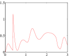
(a) Attitude error function $\Psi$

(b) Thrust at each rotor $f_{i}$ ($\mathrm{N}$)

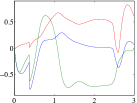
(c) Attitude error $e_{R}$ ($\mathrm{rad}$)

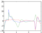
(d) Angular Velocity error $e_{\Omega}$($\mathrm{rad}/\mathrm{sec}$)

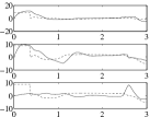
(e) Angular Velocity $\Omega$,$\Omega_{d}$ ($\mathrm{rad/s}$)

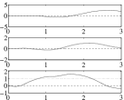
(f) Position $x$,$x_{d}$($\mathrm{m}$)

Figure 2: Flipping without adaptive term (dotted:desired, solid:actual)

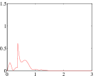
(a) Attitude error function $\Psi$

(b) Thrust at each rotor $f_{i}$ ($\mathrm{N}$)

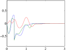
(c) Attitude error $e_{R}$ ($\mathrm{rad}$)

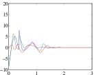
(d) Angular Velocity error $e_{\Omega}$($\mathrm{rad}/\mathrm{sec}$)

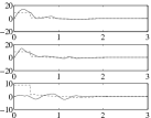
(e) Angular Velocity $\Omega$,$\Omega_{d}$ ($\mathrm{rad/s}$)

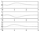
(f) Position $x$,$x_{d}$($\mathrm{m}$)

Figure 3: Flipping with adaptive term (dotted:desired, solid:actual)

Figure 4: Snapshots of a flipping maneuver: the red line denotes the rotation axis $e_{r}=[\frac{1}{\sqrt{2}},\;\frac{1}{\sqrt{2}},\;0]$. The quadrotor UAV rotates about the $e_{r}$ axis by $360^{\circ}$. The trajectory of its mass center is denoted by blue, dotted lines.

6 EXPERIMENTAL RESULTS

In this section, an experimental setup is described and the proposed geometric nonlinear controller is validated with experiments.

6.1 Hardware Description

The quadrotor UAV developed at the flight dynamics and control laboratory at the George Washington University is shown in figure 5, and its parameters are the same as described as the pervious section. The angular velocity is measured from inertial measurement unit (IMU) and the attitude is obtained from IMU data. Position of the UAV is measured from motion capture system (Vicon) and the velocity is estimated from the measurement. Ground computing system receives the Vicon data and send it to the UAV via XBee. The Gumstix is adopted as micro computing unit on the UAV. It has three main threads, namely Vicon thread, IMU thread, and control thread. The Vicon thread receives the Vicon measurement and estimates linear velocity of the quadrotor. In IMU thread, it receives the IMU measurement and estimates the attitude. The last thread handles the control outputs at each time step. Also, control outputs are calculated at 120Hz which is fast enough to run any kind of aggressive maneuvers. Information flow of the system is illustrated in Figure 6.

(a) Hardware configuration

Figure 5: Hardware development for a quadrotor UAV

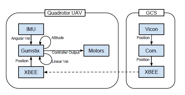
Figure 6: Information flow of overall system

6.2 Lissajous Curve Trajectory Tracking

We consider tracking of arbitrary trajectories. The following Lissajous path is chosen as desired trajectory:

$$x_{d}(t)=\begin{cases}x_{o}-\frac{t}{8}(x_{o}-x_{i})&\mbox{if }0\leqq t<8\\ [\sin(t-8)+\frac{\pi}{2}),\;\sin 2(t-8),\;-1.5]\,\mathrm{m}&\mbox{if }8\leqq t\\ \end{cases}.$$

The quadrotor takes-off from $x_{o}=[0.2,\,-2.8,\,-1.2]\mathrm{m}$ at $t=0\;\mathrm{sec}$ and flies to the initial position of the Lissajous curve trajectory where is $x_{i}=[1,\,0,\,1.5]\mathrm{m}$ by tracking a linear desired trajectory. Then, the quadrotor starts to follow the Lissajous curve trajectory at $t=8\;\mathrm{sec}$. There is about $0.15\;\mathrm{sec}$ of time delay from the Vicon motion capture system to the Gumstix. However, due to the robustness and stability properties of the proposed controller, position tracking performance shows satisfactory results as shown at Figure 7(c) and 8.

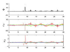
(a) Attitude error variables $\Psi,e_{R},e_{\Omega}$

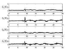
(b) Thrust of each rotor ($\mathrm{N}$)

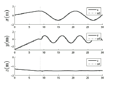
(c) Position (solid line) and desired (dotted line) $x,x_{d}$ ($\mathrm{m}$)

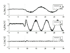
(d) Linear velocity ($\mathrm{m/sec}$)

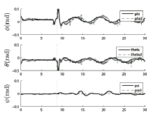
(e) Eular angles ($\mathrm{rad}$)

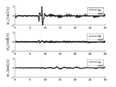
(f) Angular velocity $\Omega,\Omega_{d}$ ($\mathrm{rad/sec}$)

Figure 7: Lissajous curve trajectory tracking results (dotted:desired, solid:actual)

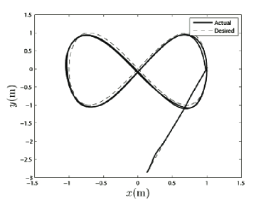
Figure 8: Lissajous curve $x-y$ plane trajectory

6.3 Flipping

Next, the proposed controller is validated with a flipping maneuver. The quadrotor takes off from a landing platform, increases altitude with constant speed to a constant point, flips $360$ degree about it $x$-axis. As presented in the numerical simulation section, this is a complex maneuver combining a nontrivial pitching maneuver with a yawing motion. It is achieved by concatenating the following two control modes of an attitude tracking same as presented in the numerical simulation to rotate the quadrotor

$$R_{d}(t)=I+\sin(4\pi t)\hat{e}_{r}+(1-\cos(4\pi t))(e_{r}e_{r}^{T}-I),$$

$$\Omega_{d}=5\pi\cdot e_{r}.$$

where $e_{r}=[1,\;0,\;0]$, and a trajectory tracking mode to make it hover after completing the preceding rotation. As it is clear from the figures, the attitude control part which handles the rotation happens in almost $0.3$ seconds and then it switched to the position control mode to make the quadrotor stabilized and hovers to the desired position. Figure 9 and 10 show the experimental results and snapshots of the flipping maneuver respectively.

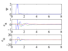
(a) Attitude error variables $\Psi,e_{R},e_{\Omega}$

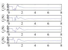
(b) Thrust of each rotor ($\mathrm{N}$)

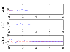
(c) Position $x,x_{d}$ ($\mathrm{m}$)

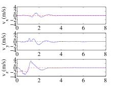
(d) Linear velocity ($\mathrm{m/sec}$)

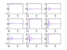
(e) Rotation Matrix

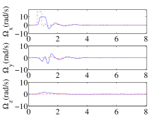
(f) Angular velocity $\Omega,\Omega_{d}$ ($\mathrm{rad/sec}$)

Figure 9: Flipping flight test results (dotted:desired, solid:actual)

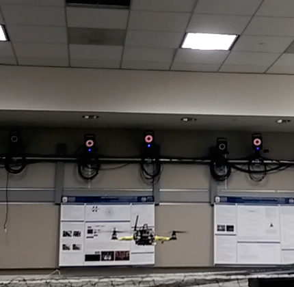
(a) $t=0.0$ sec

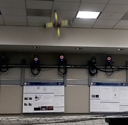
(b) $t=0.8756$ sec

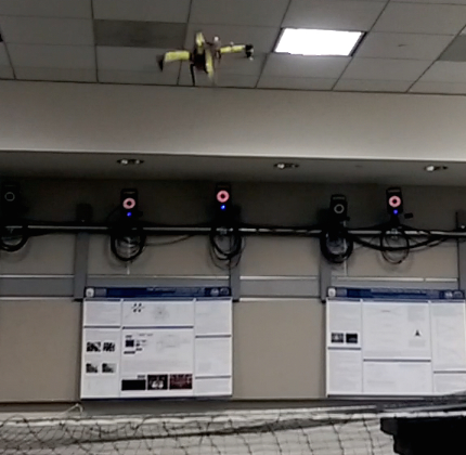
(c) $t=1.008$ sec

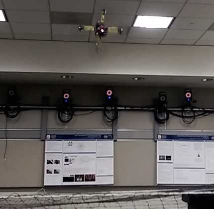
(d) $t=1.079$ sec

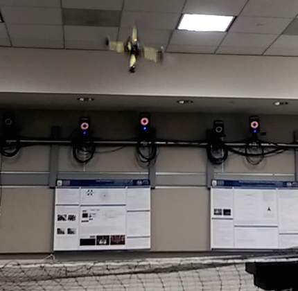
(e) $t=1.125$ sec

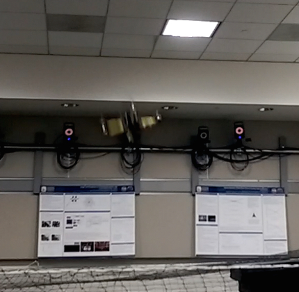
(f) $t=1.175$ sec

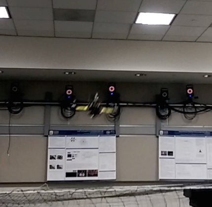
(g) $t=1.844$ sec

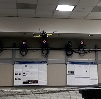
(h) $t=2.312$ sec

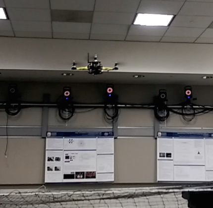
(i) $t=2.89$ sec

Figure 10: Snapshots for flipping maneuver.

7 Conclusions

A new nonlinear adaptive control system is proposed for tracking control of quadrotor unmanned aerial vehicles. It is developed directly on the special orthogonal group to avoid complexities and ambiguities that are associated with Euler-angles or quaternions, and the proposed adaptive control term guarantees almost global attractivity for the tracking error variables in the existence of uncertainties. These are verified by rigorous mathematical analysis and experiments concurrently.

This research has been supported in part by NSF under the grant CMMI-1243000 (transferred from 1029551), CMMI-1335008, and CNS-1337722.

Appendix A Proof of Proposition 1

We first find the error dynamics for $e_{R},e_{\Omega}$, and define a Lyapunov function. Then, we find conditions on control parameters to guarantee the boundedness of tracking errors. Using (3), (4), (24), the time-derivative of $Je_{\Omega}$ can be written as

$$J\dot{e}_{\Omega} =\{Je_{\Omega}+d\}^{\wedge}e_{\Omega}-k_{R}e_{R}-k_{\Omega}e_{\Omega}+\mathds{W}_{R}\tilde{\theta}_{R},$$ (33)

where $d=(2J-\mathrm{tr}[J]I)R^{T}R_{d}\Omega_{d}\in\mathbb{R}^{3}$ and $\tilde{\theta}_{R}=\theta_{R}-\bar{\theta}_{R}$. The important property is that the first term of the right hand side is normal to $e_{\Omega}$, and it simplifies the subsequent Lyapunov analysis. Define a Lyapunov function $\mathcal{V}_{2}$ be

$$\mathcal{V}_{2} =\frac{1}{2}e_{\Omega}\cdot Je_{\Omega}+k_{R}\,\Psi(R,R_{d})+c_{2}e_{R}\cdot Je_{\Omega}+\frac{1}{2\gamma_{R}}\|\tilde{\theta}_{R}\|^{2}.$$ (34)

From (12), (13), the Lyapunov function $\mathcal{V}_{2}$ is bounded as

$$z_{2}^{T}M_{21}z_{2}+\frac{1}{2\gamma_{R}}\|\tilde{\theta}_{R}\|^{2}\leq\mathcal{V}_{2}\leq z_{2}^{T}M_{22}z_{2}+\frac{1}{2\gamma_{R}}\|\tilde{\theta}_{R}\|^{2},$$ (35)

where $z_{2}=[\|e_{R}\|,\;\|e_{\Omega}\|]^{T}\in\mathbb{R}^{2}$, and the matrices $M_{12},M_{22}$ are given by

$$M_{21}=\frac{1}{2}\begin{bmatrix}k_{R}&-c_{2}\lambda_{M}\\ -c_{2}\lambda_{M}&\lambda_{m}\end{bmatrix},\,M_{22}=\frac{1}{2}\begin{bmatrix}\frac{2k_{R}}{2-\psi_{2}}&c_{2}\lambda_{M}\\ c_{2}\lambda_{M}&\lambda_{M}\end{bmatrix}.$$ (36)

From (13), the upper-bound of (35) is satisfied in the following domain:

$$D_{2}=\{(R,\Omega)\in\mathsf{SO(3)}\times\mathbb{R}^{3}\,|\,\Psi(R,R_{d})<\psi_{2}<2\}.$$ (37)

From (14), (33), the time derivative of $\mathcal{V}_{2}$ along the solution of the controlled system is given by

$$\dot{\mathcal{V}}_{2}= -k_{\Omega}\|e_{\Omega}\|^{2}+e_{\Omega}^{T}\mathds{W}_{R}\tilde{\theta}_{R}$$

$$+c_{2}\dot{e}_{R}\cdot Je_{\Omega}+c_{2}e_{R}\cdot J\dot{e}_{\Omega}+\frac{1}{\gamma_{R}}(\tilde{\theta})^{T}(\dot{\tilde{\theta}}).$$

We have $\dot{\tilde{\theta}}_{R}=-\dot{\bar{\theta}}_{R}$. Substituting (33), the above equation becomes

$$\dot{\mathcal{V}}_{2}= -k_{\Omega}\|e_{\Omega}\|^{2}+c_{2}\dot{e}_{R}\cdot Je_{\Omega}-c_{2}k_{R}\|e_{R}\|^{2}$$

$$+c_{2}e_{R}\cdot((Je_{\Omega}+d)^{\wedge}e_{\Omega}-k_{\Omega}e_{\Omega})$$

$$+\tilde{\theta}_{R}^{T}\mathds{W}_{R}^{T}(e_{\Omega}+c_{2}e_{R})-\frac{1}{\gamma_{R}}\tilde{\theta}_{R}^{T}\dot{\bar{\theta}}_{R}.$$

By substituting the adaptive law given by (16)

$$\dot{\mathcal{V}}_{2}= -k_{\Omega}\|e_{\Omega}\|^{2}+c_{2}\dot{e}_{R}\cdot Je_{\Omega}-c_{2}k_{R}\|e_{R}\|^{2}$$

$$+c_{2}e_{R}\cdot((Je_{\Omega}+d)^{\wedge}e_{\Omega}-k_{\Omega}e_{\Omega}).$$

Since $\|e_{R}\|\leq 1$, $\|\dot{e}_{R}\|\leq\|e_{\Omega}\|$, and $\|d\|\leq B_{2}$, we have

$$\dot{\mathcal{V}}_{2}\leq-z_{2}^{T}W_{2}z_{2},$$ (38)

where the matrix $W_{2}\in\mathbb{R}^{2\times 2}$ is given by

$$W_{2}=\begin{bmatrix}c_{2}k_{R}&-\frac{c_{2}}{2}(k_{\Omega}+B_{2})\\ -\frac{c_{2}}{2}(k_{\Omega}+B_{2})&k_{\Omega}-2c_{2}\lambda_{M}\end{bmatrix}.$$

Appendix B Proof of Proposition 2

We derive the tracking error dynamics and a Lyapunov function for the translational dynamics of a quadrotor UAV, and later it is combined with the stability analyses of the rotational dynamics. The subsequent analyses are developed in the domain $D_{1}$

$$D_{1}=\{ (e_{x},e_{v},R,e_{\Omega})\in\mathbb{R}^{3}\times\mathbb{R}^{3}\times\mathsf{SO(3)}\times\mathbb{R}^{3}\,|\,$$

$$\|e_{x}\|<e_{x_{\max}},\;\Psi<\psi_{1}<1\},$$ (39)

Similar to (13), we can show that

$$\frac{1}{2}\left\|e_{R}\right\|^{2}\leq\Psi(R,R_{c})\leq\frac{1}{2-\psi_{1}}\left\|e_{R}\right\|^{2}.$$ (40)

B.1 Translational Error Dynamics

The time derivative of the position error is $\dot{e}_{x}=e_{v}$. The time-derivative of the velocity error is given by

$$m\dot{e}_{v}=m\ddot{x}-m\ddot{x}_{d}=mge_{3}-fRe_{3}-m\ddot{x}_{d}+\mathds{W}_{x}\theta_{x}.$$ (41)

Consider the quantity $e_{3}^{T}R_{c}^{T}Re_{3}$, which represents the cosine of the angle between $b_{3}=Re_{3}$ and $b_{3_{c}}=R_{c}e_{3}$. Since $1-\Psi(R,R_{c})$ represents the cosine of the eigen-axis rotation angle between $R_{c}$ and $R$, we have $e_{3}^{T}R_{c}^{T}Re_{3}\geq 1-\Psi(R,R_{c})>0$ in $D_{1}$. Therefore, the quantity $\frac{1}{e_{3}^{T}R_{c}^{T}Re_{3}}$ is well-defined. To rewrite the error dynamics of $e_{v}$ in terms of the attitude error $e_{R}$, we add and subtract $\frac{f}{e_{3}^{T}R_{c}^{T}Re_{3}}R_{c}e_{3}$ to the right hand side of (41) to obtain

$$m\dot{e}_{v} =mge_{3}-m\ddot{x}_{d}-\frac{f}{e_{3}^{T}R_{c}^{T}Re_{3}}R_{c}e_{3}-X+\mathds{W}_{x}\theta_{x},$$ (42)

where $X\in\mathbb{R}^{3}$ is defined by

$$X=\frac{f}{e_{3}^{T}R_{c}^{T}Re_{3}}((e_{3}^{T}R_{c}^{T}Re_{3})Re_{3}-R_{c}e_{3}).$$ (43)

Let $A=-k_{x}e_{x}-k_{v}e_{v}-\mathds{W}_{x}\bar{\theta}_{x}-mge_{3}+m\ddot{x}_{d}$. Then, from (21), (23), we have ${b}_{3_{c}}=R_{c}e_{3}=-A/\left\|A\right\|$ and $f=-A\cdot Re_{3}$. By combining these, we obtain $f=(\left\|A\right\|R_{c}e_{3})\cdot Re_{3}$. Therefore, the third term of the right hand side of (42) can be written as

$$-\frac{f}{e_{3}^{T}R_{c}^{T}Re_{3}} R_{c}e_{3}=-\frac{(\left\|A\right\|R_{c}e_{3})\cdot Re_{3}}{e_{3}^{T}R_{c}^{T}Re_{3}}\cdot-\frac{A}{\left\|A\right\|}=A$$

$$=-k_{x}e_{x}-k_{v}e_{v}-\mathds{W}_{x}\bar{\theta}_{x}-mge_{3}+m\ddot{x}_{d}.$$

Substituting this into (42), the error dynamics of $e_{v}$ can be written as

$$m\dot{e}_{v}= -k_{x}e_{x}-k_{v}e_{v}-\mathds{W}_{x}\bar{\theta}_{x}-X+\mathds{W}_{x}{\theta}_{x}$$

$$=-k_{x}e_{x}-k_{v}e_{v}+\mathds{W}_{x}\tilde{\theta}_{x}-X.$$ (44)

where $\tilde{\theta}_{x}=\theta_{x}-\bar{\theta}_{x}$ is the estimation errors.

B.2 Lyapunov Candidate for Translation Dynamics

Let a Lyapunov candidate $\mathcal{V}_{1}$ be

$$\mathcal{V}_{1} =\frac{1}{2}k_{x}\|e_{x}\|^{2}+\frac{1}{2}m\|e_{v}\|^{2}+c_{1}e_{x}\cdot me_{v}+\frac{1}{2\gamma_{x}}\|\tilde{\theta}_{x}\|^{2}.$$ (45)

The derivative of ${\mathcal{V}}_{1}$ along the solution of (44) is given by

$$\dot{\mathcal{V}}_{1}= -(k_{v}-mc_{1})\|e_{v}\|^{2}-c_{1}k_{x}\|e_{x}\|^{2}$$

$$-c_{1}k_{v}e_{x}\cdot e_{v}+X\cdot\left\{c_{1}e_{x}+e_{v}\right\}$$

$$+\mathds{W}_{x}\tilde{\theta}_{x}\cdot\{e_{v}+c_{1}e_{x}\}-\frac{1}{\gamma_{x}}\tilde{\theta}_{x}^{T}\dot{\bar{\theta}}_{x}.$$ (46)

For the first case of the adaptive law given by (25), the last two terms of (46) are cancelled out. Also for the second case [39] that $\dot{\bar{\theta}}_{x}=\gamma_{x}(I-\frac{\bar{\theta}_{x}\bar{\theta}_{x}^{T}}{\bar{\theta}_{x}^{T}\bar{\theta}_{x}})\mathds{W}_{x}^{T}(e_{v}+c_{1}e_{x})$, we obtain

$$\dot{\mathcal{V}}_{1}= -(k_{v}-mc_{1})\|e_{v}\|^{2}-c_{1}k_{x}\|e_{x}\|^{2}$$

$$-c_{1}k_{v}e_{x}\cdot e_{v}+X\cdot\left\{c_{1}e_{x}+e_{v}\right\}$$

$$+\tilde{\theta}_{x}^{T}\frac{\bar{\theta}_{x}\bar{\theta}_{x}^{T}}{\bar{\theta}_{x}^{T}\bar{\theta}_{x}}W_{x}^{T}(e_{v}+c_{1}e_{x}).$$ (47)

In the above equation, the last term on the right hand side is always negative since $\bar{\theta}_{x}^{T}\mathds{W}_{x}^{T}(e_{v}+c_{1}e_{x})>0$ and $\tilde{\theta}_{x}^{T}\bar{\theta}_{x}\leq 0$. Therefore for both cases of (25), we obtain

$$\dot{\mathcal{V}}_{1}\leq -(k_{v}-mc_{1})\|e_{v}\|^{2}-c_{1}k_{x}\|e_{x}\|^{2}$$

$$-c_{1}k_{v}e_{x}\cdot e_{v}+X\cdot\left\{c_{1}e_{x}+e_{v}\right\}.$$ (48)

The last term of the above equation corresponds to the effects of the attitude tracking error on the translational dynamics. We find a bound of $X$, defined at (43), to show stability of the coupled translational dynamics and rotational dynamics in the subsequent Lyapunov analysis. Since $f=\|A\|(e_{3}^{T}R_{c}^{T}Re_{3})$, we have

$$\left\|X\right\|\leq \|A\|\,\|(e_{3}^{T}R_{c}^{T}Re_{3})Re_{3}-R_{c}e_{3}\|$$

$$\leq (k_{x}\|e_{x}\|+k_{v}\|e_{v}\|+B_{W_{x}}B_{\theta}+B_{1})$$

$$\times\|(e_{3}^{T}R_{c}^{T}Re_{3})Re_{3}-R_{c}e_{3}\|.$$

The last term $\|(e_{3}^{T}R_{c}^{T}Re_{3})Re_{3}-R_{c}e_{3}\|$ represents the sine of the angle between $b_{3}=Re_{3}$ and $b_{c_{3}}=R_{c}e_{3}$, since $(b_{3_{c}}\cdot b_{3})b_{3}-b_{3_{c}}=b_{3}\times(b_{3}\times b_{3_{c}})$. The magnitude of the attitude error vector, $\|e_{R}\|$ represents the sine of the eigen-axis rotation angle between $R_{c}$ and $R$ (see [29]). Therefore, $\|(e_{3}^{T}R_{c}^{T}Re_{3})Re_{3}-R_{c}e_{3}\|\leq\|e_{R}\|$ in $D_{1}$. It follows that

$$\|(e_{3}^{T}R_{d}^{T}Re_{3})Re_{3} -R_{d}e_{3}\|\leq\|e_{R}\|=\sqrt{\Psi(2-\Psi)}$$

$$\leq\left\{\sqrt{\psi_{1}(2-\psi_{1})}\triangleq\alpha\right\}<1.$$ (49)

Therefore, $X$ is bounded by

$$\left\|X\right\| \leq(k_{x}\|e_{x}\|+k_{v}\|e_{v}\|+B_{W_{x}}B_{\theta}+B_{1})\|e_{R}\|$$

$$\leq(k_{x}\|e_{x}\|+k_{v}\|e_{v}\|+B_{W_{x}}B_{\theta}+B_{1})\alpha.$$ (50)

Substituting (50) into (B.2),

$$\dot{\mathcal{V}}_{1} \leq-(k_{v}(1-\alpha)-mc_{1})\|e_{v}\|^{2}-{c_{1}k_{x}}(1-\alpha)\|e_{x}\|^{2}$$

$$+{c_{1}k_{v}}(1+\alpha)\|e_{x}\|\|e_{v}\|$$

$$+\|e_{R}\|\left\{(B_{W_{x}}B_{\theta}+B_{1})({c_{1}}\|e_{x}\|+\|e_{v}\|)+k_{x}\|e_{x}\|\|e_{v}\|\right\}.$$ (51)

In the above expression for $\dot{\mathcal{V}}_{1}$, there is a third-order error term, namely $k_{x}\|e_{R}\|\|e_{x}\|\|e_{v}\|$. Using (49), it is possible to choose its upper bound as $k_{x}\alpha\|e_{x}\|\|e_{v}\|$ similar to other terms, but the corresponding stability analysis becomes complicated, and the initial attitude error should be reduced further. Instead, we restrict our analysis to the domain $D_{1}$ defined in (39), and its upper bound is chosen as $k_{x}e_{x_{\max}}\|e_{R}\|\|e_{v}\|$.

B.3 Lyapunov Candidate for the Complete System

Let $\mathcal{V}=\mathcal{V}_{1}+\mathcal{V}_{2}$ be the Lyapunov candidate of the complete system. Define $z_{1}=[\|e_{x}\|,\;\|e_{v}\|]^{T}$, $z_{2}=[\|e_{R}\|,\;\|e_{\Omega}\|]^{T}\in\mathbb{R}^{2}$, and

$$\mathcal{V}_{A}=\frac{1}{2\gamma_{x}}\|\theta_{x}-\bar{\theta}_{x}\|^{2}+\frac{1}{2\gamma_{R}}\|\theta_{R}-\bar{\theta}_{R}\|^{2}.$$

Using (40), the bound of the Lyapunov candidate $\mathcal{V}$ can be written as

$$z_{1}^{T}M_{11}z_{1}+z_{2}^{T}M_{21}z_{2} +\mathcal{V}_{A}\leq\mathcal{V}\leq z_{1}^{T}M_{12}z_{1}+z_{2}^{T}M^{\prime}_{22}z_{2}+\mathcal{V}_{A},$$ (52)

where the matrices $M_{11},M_{12},M_{21},M_{22}$ are given by

$$M_{11}=\frac{1}{2}\begin{bmatrix}k_{x}&-mc_{1}\\ -mc_{1}&m\end{bmatrix},\;M_{12}=\frac{1}{2}\begin{bmatrix}k_{x}&mc_{1}\\ mc_{1}&m\end{bmatrix},$$

$$M_{21}=\frac{1}{2}\begin{bmatrix}k_{R}&-c_{2}\lambda_{M}\\ -c_{2}\lambda_{M}&\lambda_{m}\end{bmatrix},\;M_{22}=\frac{1}{2}\begin{bmatrix}\frac{2k_{R}}{2-\psi_{1}}&c_{2}\lambda_{M}\\ c_{2}\lambda_{M}&\lambda_{M}\end{bmatrix}.$$

Using (38) and (51), the time-derivative of $\mathcal{V}$ is given by

$$\dot{\mathcal{V}} \leq-z_{1}^{T}W_{1}z_{1}+z_{1}^{T}W_{12}z_{2}-z_{2}^{T}W_{2}z_{2}\leq-z^{T}Wz$$ (53)

where $z=[z_{1},z_{2}]^{T}\in\mathbb{R}^{2}$, and the matrices $W_{1},W_{12},W_{2}\in\mathbb{R}^{2\times 2}$ are defined at (29)-(31). The matrix $W\in\mathbb{R}^{2\times 2}$ is given by

$$W=\begin{bmatrix}\lambda_{m}(W_{1})&-\frac{1}{2}\|W_{12}\|_{2}\\ -\frac{1}{2}\|W_{12}\|_{2}&\lambda_{m}(W_{2})\end{bmatrix}.$$

The conditions given at (18), (27), (28) guarantee that all of matrices $M_{11},M_{12},M_{21},M_{22},W$ are positive definite.

Appendix C Proof of Proposition 3

According to the proof of Proposition 1, the attitude tracking errors asymptotically decrease to zero, and therefore, they enter the region given by (26) in a finite time $t^{*}$, after which the results of Proposition 2 can be applied to yield attractiveness. The remaining part of the proof is showing that the tracking error $z_{1}=[\|e_{x}\|,\|e_{v}\|]^{T}$ is bounded in $t\in[0,t^{*}]$. This is similar to the proof given at [17].

References

- [1] Mahony, R., Kumar, V., and Corke, P., 2012. “Multirotor aerial vehicles”. IEEE Robot. Automat. Mag, 19, pp. 20–32.
- [2] Goodarzi, F. A., Lee, D., and Lee, T., 2014. “Geometric stabilization of quadrotor UAV with a payload connected by flexible cable”. In Proceedings of American Control Conference.
- [3] Cabecinhas, D., Cunha, R., and Silvestre, C., 2009. “Rotorcraft path following control for extended flight envelope coverage”. In Proceedings of the IEEE Conference on Decision and Control, pp. 3460–3465.
- [4] Mellinger, D., and Kumar, V., 2011. “Minimum snap trajectory generation and control for quadrotors”. In Proceedings of the International Conference on Robotics and Automation.
- [5] Naldi, R., Marconi, L., and Gentili, L., 2009. “Robust takeoff and landing for a class of aerial robots”. In Proceedings of the IEEE Conference on Decision and Control, pp. 3436–3441.
- [6] Hua, M., Hamel, T., Morin, P., and Samson, C., 2009. “A control approach for thrust-propelled underactuated vehicles and its application to VTOL drones”. IEEE Transactions on Automatic Control, 54(8), pp. 1834–1853.
- [7] Johnson, N. L., and Leang, K. K., 2013. “Enhanced proportional-derivative control of a micro quadcopter”. In ASME 2013 Dynamic Systems and Control Conference.
- [8] M. Hassan Tanveer, S. Faiz Ahmed, D. H. M. K. J., and Warsi, F. A., 2013. “Disturbance and noise rejection controller design for smooth takeoff / landing and altitude stabilization of quad-rotor”. Journal of Applied Sciences Research, 5(9).
- [9] L na ck Besnard, Y. B. S., and Landrum, B., 2007. “Control of a quadrotor vehicle using sliding mode disturbance observer”. In Proceedings of the 2007 American Control Conference.
- [10] Hossein Bolandi, Mohammad Rezaei, R. M. H. N., and Smailzadeh, S. M., 2013. “Attitude control of a quadrotor with optimized pid controller”. Intelligent Control and Automation(4).
- [11] Sharma, A., and Barve, P. A., 2012. “Controlling of quad-rotor uav using pid controller and fuzzy logic controller”. International Journal of Electrical, Electronics and Computer Engineering, 1(2), pp. 38–41.
- [12] Chao Liu, Sheng Jing Tang, S. Y. Y., and Guo, J., 2013. “Fuzzy sliding-mode control for quad-rotor trajectory tracking”. The international journal of Unmanned System Technology, 278, pp. 1593–1600.
- [13] Addy Wahyudie, T. B. S., and Noura, H., 2013. “Robust pid controller for quad-rotors”. The international journal of Unmanned System Technology, 1(1).
- [14] Hoffmann, G., Huang, H., Waslander, S., and Tomlin, C., 2007. “Quadrotor helicopter flight dynamics and control: Theory and experiment”. In Proceedings of the AIAA Guidance, Navigation, and Control Conference. AIAA 2007-6461.
- [15] Castillo, P., Albertos, P., Garcia, P., and Lozano, R., 2006. “Simple real-time attitude stabilization of a quadrotor aircraft with bounded signals”. In Proceeding of the IEEE Conference on Decision and Control.
- [16] Lee, T., Leok, M., and McClamroch, N., 2012. “Nonlinear robust tracking control of a quadrotor UAV on SE(3)”. In Proceeding of the American Control Conference, pp. 4649–4654.
- [17] Lee, T., Leok, M., and McClamroch, N., 2013. “Nonlinear robust tracking control of a quadrotor UAV on ”. Asian Journal of Control, 15(2), Mar., pp. 391–408.
- [18] Dydek, Z., Annaswamy, A., and Lavretsky, E., 2012. “Adaptive control of quadrotor uavs: A design trade study with flight evaluations”. IEEE Transactions on Control Systems Technology, 21(4).
- [19] Selfridge, J. M., and Tao, G., 2014. “A multivariable adaptive controller for a quadrotor with guaranteed matching conditions”. Systems Science and Control Engineering An Open Access Journal, 2, pp. 24–33.
- [20] Gianluca Antonelli, Filippo Arrichiello, S. C., and Giordano, P. R., 2013. “Adaptive trajectory tracking for quadrotor mavs in presence of parameter uncertainties and external disturbances”. In IEEE/ASME International Conference on Advanced Intelligent Mechatronics (AIM).
- [21] Zhen, H., Qi, X., and Dong, H., 2013. An Adaptive Block Backstepping Controller for Attitude Stabilization of a Quadrotor Helicopter, Vol. 8 of 2. Transactions on Systems and Control, april.
- [22] Cabecinhas, D., Cunha, R., and Silvestre, C., 2014. “A nonlinear quadrotor trajectory tracking controller with disturbance rejection”. Control Engineering Practice, 26, pp. 1–10.
- [23] Lee, D., Kim, H., and Sastry, S., 2009. “Feedback linearization vs. adaptive sliding mode control for a quadrotor helicopter”. Int. Journal of Control, Automation and Systems, 7, pp. 1–10.
- [24] B. J. Bialy, J. Klotz, K. B., and Dixon, W. E., 2013. “Lyapunov-based robust adaptive control of a quadrotor uav in the presence of modeling uncertainties”. In Proceeding of American Control Conference (ACC 2013).
- [25] Mellinger, D., Michael, N., and Kumar, V., 2012. “Trajectory generation and control for precise aggressive maneuvers with quadrotors”. International Journal Of Robotics Research, 31(5), pp. 664–674.
- [26] Tayebi, A., and McGilvray, S., 2006. “Attitude stabilization of a VTOL quadrotor aircraft”. IEEE Transactions on Control System Technology, 14(3), pp. 562–571.
- [27] Bhat, S., and Bernstein, D., 2000. “A topological obstruction to continuous global stabilization of rotational motion and the unwinding phenomenon”. Systems and Control Letters, 39(1), pp. 66–73.
- [28] Mayhew, C., Sanfelice, R., and Teel, A., 2011. “Quaternion-based hybrid control for robust global attitude tracking”. IEEE Transactions on Automatic Control, 56(11), pp. 2555–2566.
- [29] Lee, T., Leok, M., and McClamroch, N., 2010. “Geometric tracking control of a quadrotor UAV on SE(3)”. In Proceedings of the IEEE Conference on Decision and Control, pp. 5420–5425.
- [30] Goodarzi, F., Lee, D., and Lee, T., 2013. “Geometric nonlinear PID control of a quadrotor UAV on SE(3)”. In in Proceedings of the European Control Conference, pp. 3845–3850.
- [31] Chaturvedi, N., Sanyal, A., and McClamroch, N., 2011. “Rigid-body attitude control”. IEEE Control Systems Magazine, 31(3), pp. 30–51.
- [32] Gillula, J., Hoffmann, G., Huang, H., Vitus, M., and Tomlin, C., 2011. “Applications of hybrid reachability analysis to robotic aerial vehicles”. The International Journal of Robotics Research, 30(3), pp. 335–354.
- [33] Castillo, P., Lozano, R., and Dzul, A., 2005. “Stabilization of a mini rotorcraft with four rotors”. IEEE Control System Magazine, pp. 45–55.
- [34] Bullo, F., and Lewis, A., 2005. Geometric control of mechanical systems, Vol. 49 of Texts in Applied Mathematics. Springer-Verlag, New York. Modeling, analysis, and design for simple mechanical control systems.
- [35] Lee, T., 2013. “Robust adaptive tracking on with an application to the attitude dynamics of a quadrotor UAV”. IEEE Transactions on Control Systems Technology, 21(5), pp. 1924–1930.
- [36] Subbarao, K., 2004. “Nonlinear PID-like controllers for rigid-body attitude stabilization”. Journal of the Astronautical Sciences, 52(1-2), pp. 61–74.
- [37] Subbarao, K., and Akella, M., 2004. “Differentiator-free nonlinear proportional-integral controllers for rigid-body attitude stabilization”. Journal of Guidance, Control, and Dynamics, 27(6), pp. 1092–1096.
- [38] Show, L., Juang, J., Lin, C., and Jan, Y., 2002. “Spacecraft robust attitude tracking design: PID control approach”. In Proceeding of the American Control Conference, 1360-1365, ed.
- [39] Ioannou, P. A., 1996. Robust Adaptive Control. PTR Prentice-Hall.