One–Loop Dominance in the Imaginary Part of the Polarizability:
Application to Blackbody and Non–Contact van der Waals Friction

Abstract

Phenomenologically important quantum dissipative processes include black-body friction (an atom absorbs counterpropagating blue-shifted photons and spontaneously emits them in all directions, losing kinetic energy) and non-contact van der Waals friction (in the vicinity of a dielectric surface, the mirror charges of the constituent particles inside the surface experience drag, slowing the atom). The theoretical predictions for these processes are modified upon a rigorous quantum electrodynamic (QED) treatment, which shows that the one-loop “correction” yields the dominant contribution to the off-resonant, gauge-invariant, imaginary part of the atom’s polarizability at room temperature, for typical atom-surface interactions. The tree-level contribution to the polarizability dominates at high temperature.

Introduction.—Can a physical object experience friction effects, even if it is not in contact with a surface, i.e., even if the overlap of the wave function of the atom with the surface is negligible? This question has intrigued physicists for the last three decades, and the precise functional form of the non-contact friction of an atom-surface interaction has been discussed controversially in the literature Levitov (1989); Polevoi (1990); Hoye and Brevik (1992); *HoBr1993; Mkrtchian (1995); Tomassone and Widom (1997); Persson and Zhang (1998); Dedkov and Kyasov (1999); *DeKy2001; *DeKy2002; *DeKy2002review; Volokitin and Persson (1999); *VoPe2001; *VoPe2002; *VoPe2003; *VoPe2005; *VoPe2006; *VoPe2007; *VoPe2008; Dorofeyev et al. (2001). Intuitively, if an ion moves parallel to a surface, at a distance a few (hundred) nanomenters, then it is quite natural to assume that the motion of the mirror charge inside the material leads to Ohmic heating and thus, to a commensurate energy loss (friction force) acting on the atom flying by. The corresponding effect for a neutral atom is less obvious to analyze, but one may argue that the thermal fluctuations of the electric dipole moment of the atom may induce corresponding fluctuations of the mirror charge(s) of the constituent particles of the atom inside the material, again leading to Ohmic heating. The derivation relies heavily on the quantum statistical theory of thermal fluctuations of the electromagnetic field near a surface, and on the fluctuation-dissipation theorem Pitaevskii and Lifshitz (1958); Kubo (1966); Tomassone and Widom (1997). For non-contact friction in the zero-temperature limit, even the existence of the effect still is subject to scientific debate Pendry (1997); Philbin and Leonhardt (2009); *Pe2010; *Le2010comment; *Pe2010reply; Volokitin and Persson (2011); Despoja et al. (2011). Ultimately, non-contact friction effects limit the extent to which friction forces Singer and Pollock (1992); *Pe1998friction can be reduced in an experiment. These limits are important for three-dimensional atomic imaging Sidles et al. (1995); *DoFuWeGo1998; *GoFu2001; *StEtAl2001; *MaRu2001; *HoEtAl2001, tests of gravitational interactions at small length scales Arkani-Hamed et al. (1998), limits of magnetic resonance force microscopy Rugar et al. (2004), and they affect the behavior of micro-electro-mechanical systems (MEMS) at the nanometer scale Buks and Roukes (2001); *ChEtAl2001science; *ChEtAl2001prl.

Complementing the effect non-contact friction, the drag exerted by oncoming blue-shifted thermal blackbody radiation on a moving atom has recently been analyzed for nonrelativistic neutral atoms as they travel through space Mkrtchian et al. (2003); Maia Neto and Farina (2004); Mkrtchian et al. (2004); Łach et al. (2012). Both the blackbody as well as the non-contact quantum (thermal) friction require as input the imaginary part of the atom’s polarizability, whose precise functional form for small driving frequencies is different depending on whether one uses (i) resonant Dirac-$\delta$ peaks Mkrtchian et al. (2003), or the (ii) length-gauge or (iii) velocity-gauge expressions in the low-frequency limit (see Chap. XXI of Ref. Messiah (1962) and Ref. Łach et al. (2012)). Any theoretical prediction crucially depends on a resolution of the “gauge puzzle”, which is the subject of the current Letter. Quite surprisingly, a separation of the problem in terms of a rigorous quantum electrodynamic approach to the atom Bethe and Salpeter (1957) leads to a natural separation of the resonant and the non-resonant (one-loop) effects. Perhaps even more surprisingly, the one-loop correction here dominates over the tree-level term, for typical materials and temperatures.

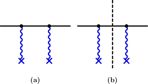
Figure 1: (Color online.) The Feynman diagram for the ac Stark shift involves the absorption or emission of two laser photons by the atom [Fig. (a)]. A tree-level imaginary part (cut of the diagram, see Fig. (b)] is generated only if the absorbed laser photon happens to be at resonance with regard to a transition of the atom to an excited state [see Eq. (12)].

Imaginary Part of the Polarizability.—The calculation of the imaginary part of the polarizability relies on the following two observations. (i) One identifies the main contribution to the imaginary part of the polarizability with the imaginary part of an energy shift, namely, the ac Stark shift Haas et al. (2006). In second quantization, the ac Stark shift in a laser field can be formulated in terms of the virtual transitions of a reference state (atom in the state $|\phi_{0}\rangle$, and $n_{L}$ laser photons), to a virtual state with the atom in the virtual state $|\phi_{m}\rangle$, and $n_{L}\pm 1$ laser photons. (ii) One observes that the imaginary part is generated by an additional virtual photon loop (self-energy insertion) which is cut in the middle of the diagram, with a virtual state that brings the atom back to the reference state $|\phi_{0}\rangle$, has $n_{L}-1$ laser photons (one laser photon has been absorbed) and one spontaneously emitted photon, with wave vector $\vec{k}$, polarization $\lambda$, and an energy $\omega_{\vec{k}\lambda}=\omega_{L}$.

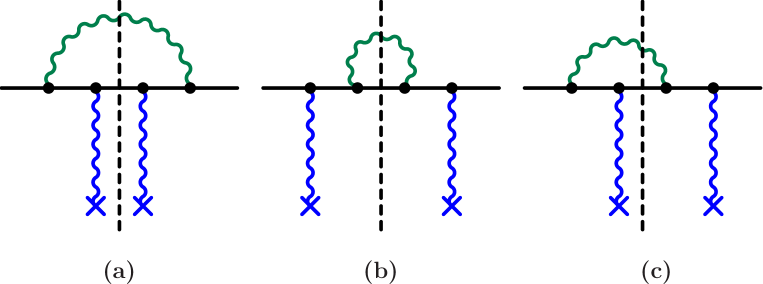
Figure 2: (Color online.) The radiative correction to the ac Stark shift involves an additional virtual photon loop (green). The imaginary part (cut of the diagram) is generated when the virtual photon becomes real, i.e., when the laser photon has the same energy as the spontaneously emitted photon.

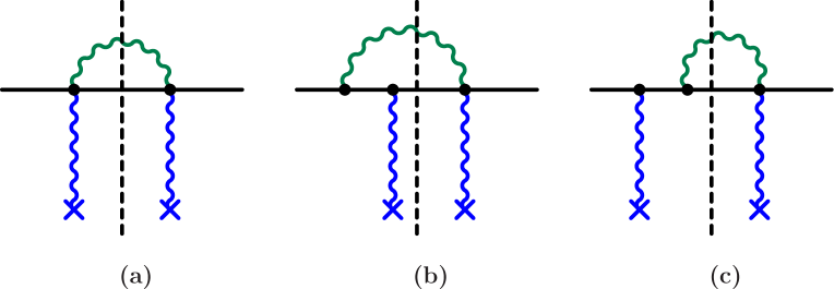
Figure 3: (Color online.) In velocity gauge, the seagull term leads to additional diagrams with a two-photon vertex.

The Feynman diagram for the ac Stark shift is given in Fig. 1. The reference state is $|\phi_{0}\rangle=|\phi,n_{L},0\rangle$, with the atom in the state $|\phi\rangle$, $n_{L}$ laser photons and zero photons in other modes. The energy eigenvalue of the unperturbed reference state is $H_{Q}\,|\phi_{0}\rangle=E_{0}\,|\phi_{0}\rangle$, with $E_{0}=E+\hbar\,n_{L}\,\omega_{L}$, where $H_{Q}$ is the sum of the atomic (A) and the electromagnetic (EM) field Hamiltonians,

$$H_{Q}= \;H_{A}+H_{EM}\,,\quad H_{A}=\sum_{m}E_{m}\,|\phi_{m}\rangle\,\langle\phi_{m}|\,,$$ (1a)

$$H_{EM}= \;\sum_{\vec{k}\,\lambda\neq L}\hbar\,\omega_{\vec{k}\,\lambda}a_{\vec{k}\,\lambda}^{+}\;a_{\vec{k}\,\lambda}+\hbar\,\omega_{L}\;a^{+}_{L}\;a_{L}\,,$$ (1b)

where $L$ denotes the laser mode, and the photon creation and annihilation operators are $a^{+}$ and $a$, respectively Cohen-Tannoudji et al. (1978a, b). If the laser photon of angular frequency $\omega_{L}$ is resonant with respect to an atomic transition, then the absorption of a laser photon may deplete the reference state, leading to a transition to a state $|\phi_{r}\rangle=|\phi_{m},n_{L}-1,0\rangle$, provided $\hbar\,\omega_{L}=E_{m}-E$, where $E$ is the atomic reference state energy. However, when the absorption of a laser photon is accompanied by the spontaneous emission of another photon, then a transition to a final state $|\phi_{f}\rangle=|\phi,n_{L}-1,1_{\vec{k}\,\lambda}\rangle$ becomes possible, where the laser fields retains $n_{L}-1$ photons, while one photon is emitted into the mode $\vec{k}\,\lambda$ (the state is $|1_{\vec{k}\,\lambda}\rangle$ in the occupation number notation). The imaginary part of the ac Stark shift due to the diagrams in Fig. 2 is due to the dipole interaction $H_{L}$ ($z$-polarized laser) and the interaction Hamiltonian $H_{I}$ (other field modes),

$$\vec{E}_{L}= \;\hat{e}_{z}\,\sqrt{\frac{\hbar\omega_{L}}{2\epsilon_{0}{\mathcal{V}}_{L}}}\,\left(a_{L}+a_{L}^{+}\right)=\hat{e}_{z}\,E_{L}\,,$$ (2a)

$$\vec{E}= \;\sum_{\vec{k}\,\lambda}\sqrt{\frac{\hbar\omega_{\vec{k}\,\lambda}}{2\epsilon_{0}{\mathcal{V}}}}\,\hat{\epsilon}_{\vec{k}\,\lambda}\left(a_{\vec{k}\,\lambda}+a_{\vec{k}\,\lambda}^{+}\right)\,,$$ (2b)

$$H_{L}= \;-e\,z\,E_{L}\,,\qquad H_{I}=-e\,\vec{r}\cdot\vec{E}\,.$$ (2c)

Here, the normalization volumes are ${\mathcal{V}}$ for the quantized field, and ${\mathcal{V}}_{L}$ for the laser field. We can write

$$I_{L}=\frac{n_{L}\,\hbar\omega_{L}\,c}{{\mathcal{V}}_{L}}\,,\qquad\sum_{\vec{k}}={\mathcal{V}}\,\int\frac{{\mathrm{d}}^{3}k}{(2\pi)^{3}}\,,$$ (3)

for the laser field intensity $I_{L}$ and the matching of the sum over available photon modes $\sum_{\vec{k}}$ to the integral $\int{\mathrm{d}}^{3}k$ over the continuum. Second-order perturbation theory for the reference state $|\phi_{0}\rangle$ leads to Haas et al. (2006)

$$\delta E^{(2)}= \;-\left<H_{L}\,G^{\prime}(E_{0})\,H_{L}\right>=-\frac{I_{L}}{2\epsilon_{0}\,c}\,\alpha(\omega_{L})\,,$$ (4a)

$$\alpha(\omega_{L})= \;e^{2}\,\sum_{\pm}\left<\phi\left|z\,G_{A}(E\pm\omega_{L})\,z\right|\phi\right>$$

$$= \;\frac{e^{2}}{3}\,\sum_{\pm}\left<\phi\left|x^{i}\,G_{A}(E\pm\omega_{L})\,x^{i}\right|\phi\right>\,,$$ (4b)

where $G^{\prime}(z)=[1/(H_{Q}-z)]^{\prime}$ is the reduced Green function for atom$+$field (with the reference state $|\phi_{0}\rangle$ excluded), while $G_{A}(z)=[1/(H_{A}-z-{\mathrm{i}}\,\epsilon)]$ is the atomic Green function. The “reduction” of the Green function excludes the combined atom$+$field state $|\phi_{0}\rangle$ but not the atomic reference state $|\phi\rangle$. We assume that the atom’s reference state is spherically symmetric. The fourth-order energy shift leads to the diagrams shown in Fig. 2,

$$\delta E^{(4)}=-\left<H_{I}\,G^{\prime}(E_{0})\,H_{L}\,G^{\prime}(E_{0})\,H_{L}\,G^{\prime}(E_{0})\,H_{I}\right>$$

$$\;-\left<H_{L}\,G^{\prime}(E_{0})\,H_{I}\,G^{\prime}(E_{0})\,H_{I}\,G^{\prime}(E_{0})\,H_{L}\right>$$

$$\;-2\,\left<H_{I}\,G^{\prime}(E_{0})\,H_{L}\,G^{\prime}(E_{0})\,H_{I}\,G^{\prime}(E_{0})\,H_{L}\right>\,,$$ (5)

The three terms in Eq. (One–Loop Dominance in the Imaginary Part of the Polarizability: Application to Blackbody and Non–Contact van der Waals Friction) correspond to the diagrams in Fig. 2(a), (b), (c), respectively. Let us consider the energy shift due to the diagram in Fig. 2(a),

$$\delta E_{a}= \;-e^{4}\sum_{\vec{k}\,\lambda}\frac{\hbar\omega_{L}}{2\epsilon_{0}{\mathcal{V}}_{L}}\frac{\hbar\omega_{\vec{k}\,\lambda}}{2\epsilon_{0}{\mathcal{V}}}\left<\phi_{0}\left|(\hat{\epsilon}_{\vec{k}\,\lambda}\cdot\vec{r})\left(a_{\vec{k}\,\lambda}^{+}+a_{\vec{k}\,\lambda}\right)\ \right.\right.$$

$$\;\times\;G^{\prime}(E_{0})\;z\,(a_{L}^{+}+a_{L})\;G^{\prime}(E_{0})\;z\,(a_{L}^{+}+a_{L})\,$$

$$\;\left.\left.\times\;G^{\prime}(E_{0})\,(\hat{\epsilon}_{\vec{k}\,\lambda}\cdot\vec{r})\,\left(a_{\vec{k}\,\lambda}^{+}+a_{\vec{k}\,\lambda}\right)\ \right|\phi_{0}\right>.$$ (6)

In order to calculate the imaginary part, one isolates the terms which correspond to the absorption from the laser field and emission into the spontaneous mode. Using the matching condition (3) and summing over the polarizations of the spontaneously emitted photon, one obtains

$$\delta E_{a}\sim \;-e^{4}\int\frac{{\mathrm{d}}^{3}k}{(2\pi)^{3}}\,\frac{I_{L}}{2\epsilon_{0}c}\,\frac{\hbar\omega_{\vec{k}\,\lambda}}{2\epsilon_{0}}\left(\delta^{ij}-\frac{k^{i}\,k^{j}}{\vec{k}^{\,2}}\right)$$

$$\;\times\left<\phi\left|z\,G_{A}(E-\omega_{\vec{k}\,\lambda})\,x^{i}\,G_{A}(E+\omega_{L}-\omega_{\vec{k}\,\lambda})\,\right.\right.$$

$$\;\left.\left.\times x^{j}\,G_{A}(E-\omega_{\vec{k}\,\lambda})\,z\,\right|\phi\right>\,.$$ (7)

The imaginary part due to the transition into the state $|\phi_{f}\rangle$ can be extracted from the relation $1/(x-{\mathrm{i}}\epsilon)\to\mbox{(P.V.)}(1/x)+{\mathrm{i}}\,\pi\,\delta(x)$, i.e., by projecting

$$G_{A}(E+\omega_{L}-\omega_{\vec{k}\,\lambda})\to\frac{{\mathrm{i}}\,\pi}{\hbar}\,\delta(\omega_{\vec{k}\,\lambda}-\omega_{L})\;|\phi\rangle\,\langle\phi|\,.$$ (8)

One finally obtains

$${\rm Im}(\delta E_{a})=-\frac{I_{L}}{2\epsilon_{0}c}\frac{\omega^{3}_{L}}{6\pi\epsilon_{0}c^{3}}\left[\frac{e^{2}}{3}\left<\phi\left|x^{i}G_{A}(E-\omega_{L})x^{i}\right|\phi\right>\right]^{2}$$ (9)

and after summing up the diagrams in Fig. 2(a), (b) and (c), the result is

$${\rm Im}(\delta E^{(4)})= \;-\frac{I_{L}}{2\epsilon_{0}c}\frac{\omega^{3}_{L}}{6\pi\epsilon_{0}c^{3}}\left[\frac{e^{2}}{3}\left<\phi\left|x^{i}G_{A}(E-\omega_{L})x^{i}\right|\phi\right>\right.$$

$$\;\left.+\frac{e^{2}}{3}\left<\phi\left|x^{j}G_{A}(E+\omega_{L})x^{j}\right|\phi\right>\right]^{2},$$ (10)

so that ${\rm Im}(\delta E^{(4)})=-{\textstyle{\frac{I_{L}}{2\epsilon_{0}c}}}\,{\textstyle{\frac{\omega^{3}_{L}}{6\pi\epsilon_{0}c^{3}}}}\left[\alpha(\omega_{L})\right]^{2}$. Matching with the second-order ac Stark shift given in Eq. (4), and adding the resonant contribution [Fig. 1(b)], one obtains

$${\rm Im}[\alpha(\omega_{L})]={\rm Im}[\alpha_{R}(\omega_{L})]+\frac{\omega^{3}_{L}}{6\pi\epsilon_{0}c^{3}}\,[\alpha(\omega_{L})]^{2}\,.$$ (11)

Here, ${\rm Im}\left[\alpha_{R}(\omega_{L})\right]={\rm Im}\left[\alpha_{r}(\omega_{L})\right]-{\rm Im}\left[\alpha_{r}(-\omega_{L})\right]$ where

$${\rm Im}\left[\alpha_{r}(\omega_{L})\right]=\frac{\pi}{2}\,\sum_{m}\frac{f_{m0}}{E_{m}-E}\,\delta(E_{m}-E+\hbar\,\omega_{L})$$ (12)

is the resonant contribution sym . The dipole oscillator strength $f_{m0}$ reads as $f_{m0}={\textstyle{\frac{2}{3}}}\,e^{2}\,(E_{m}-E)\,|\langle\phi|x^{i}|\phi_{m}\rangle|^{2}$ (see Ref. Yan et al. (1996)). The result (11) allows us to unify the formulas given in Eqs. (G2) and (G3) of Ref. Zurita-Sanchez et al. (2004), Eq. (49) of Ref. Boyer (1969) and Eq. (15.83) of Novotny and Hecht (2012), into a single, compact result. Namely, the appearance of the square of the polarizability is otherwise ascribed to a radiative reaction force Boyer (1969); Zurita-Sanchez et al. (2004), but finds a natural interpretation within a quantum electrodynamic (QED) formalism. The resonant contribution is the tree-level term in QED.

In velocity gauge, one replaces for the dipole coupling $-e\,\vec{r}\cdot\vec{E}$ by $-e\,\vec{p}\cdot\vec{A}/m_{e}$, where $m_{e}$ is the electron mass. From the diagrams in Fig. 2, one then obtains the energy shift given in Eq. (One–Loop Dominance in the Imaginary Part of the Polarizability: Application to Blackbody and Non–Contact van der Waals Friction), but with the replacement $\omega_{L}^{3}\to\omega_{L}$ in the prefactor, and $x^{i}\to p^{i}/m_{e}$ in the dipole matrix elements. The resulting expression is not identical to the length-gauge result (11) but there are additional diagrams to consider, given in Fig. 3, which involve the seagull Hamiltonian, proportional to the square of the vector potential. Using the commutator relation $p^{i}={\mathrm{i}}\,m_{e}\,[H-E+\omega_{L},r^{i}]$ repeatedly, one can show that the additional terms from the diagrams in Fig. 3 restore the full gauge invariance of the result (11).

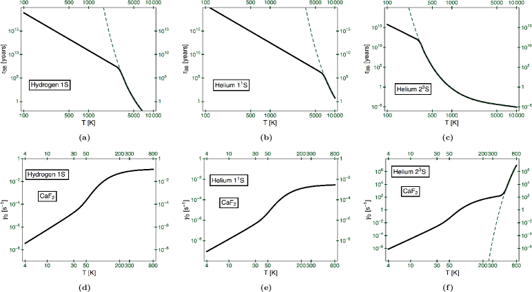
Figure 4: (Color online.) Theoretical predictions [Figs. (a)–(c)] for the attenuation time $\tau_{\rm BB}$ (equal to the ratio of atomic mass to $\eta_{\rm BB}$) are displayed for blackbody radiation friction. For CaF₂ van der Waals friction [see Figs. (d)–(f)], the coefficient $\gamma_{0}$ is defined in Eq. (17). The dashed lines in Figs. (a)–(c), and (f), are obtained with the tree-level term given in Eq. (12).

Numerical Evaluation.—We are concerned with the numerical evaluation of the blackbody friction integral (restoring SI mksA units)

$$\eta_{\rm BB}=\frac{\beta\hbar^{2}}{12\pi^{2}\,\epsilon_{0}\,c^{5}}\,\int\limits_{0}^{\infty}\frac{{\mathrm{d}}\omega\,\omega^{5}\;{\rm Im}[\alpha(\omega)]}{\sinh^{2}({\textstyle{\frac{1}{2}}}\beta\hbar\omega)}\,,$$ (13)

which determines the blackbody radiation force $F=-\eta\,v$, and the non-contact friction integral (in SI mksA)

$$\eta_{\rm QF}= \;\frac{3\beta\hbar^{2}}{32\pi^{2}\epsilon_{0}{\mathcal{Z}}^{5}}\,\int\limits_{0}^{\infty}\frac{{\mathrm{d}}\omega\,{\rm Im}[\alpha(\omega)]}{\sinh^{2}({\textstyle{\frac{1}{2}}}\beta\hbar\omega)}{\rm Im}\left[\frac{\epsilon(\omega)-1}{\epsilon(\omega)+1}\right]\,,$$ (14)

for interactions with a dielectric. Here, $\beta=1/(k_{B}\,T)$ is the Boltzmann factor, ${\mathcal{Z}}$ is the distance to the wall, and $\epsilon_{0}$ is the vacuum permittivity.

For low temperatures ($\beta\to\infty$), only small frequencies contribute to the friction forces and the imaginary part of the polarizability can be approximated as ${\rm Im}[\alpha(\omega)]\approx\omega^{3}[\alpha(0)]^{2}/(6\pi\epsilon_{0}c^{3})$ Here, $\alpha(0)$ is the static polarizability of the atom, i.e., the low-frequency limit, where the resonant contribution in Eq. (11) can be neglected. Thus, the blackbody friction coefficient goes as $T^{8}$ for small temperatures,

$$\eta_{\rm BB}\approx\frac{32\,\pi^{5}\,\left.\alpha(0)\right|_{{\rm SI}}^{2}}{135\,\hbar^{7}\,\epsilon_{0}^{2}\,c^{8}\,\beta^{8}}=\frac{512\,\pi^{7}\,\left.\alpha(0)\right|_{{\rm a.u.}}^{2}}{135\,\alpha^{6}\,\hbar\,m_{e}^{6}\,c^{14}\,\beta^{8}}\,.$$ (15)

The subscript of the static polarizability indicates the system of units. In atomic units, the subscript a.u. indicates the reduced quantity, i.e., the “numerical value” Bethe and Salpeter (1957); Mohr et al. (2012). The polarizability is normally given in atomic units in the literature Pachucki and Sapirstein (2000); Masili and Starace (2003); Łach et al. (2004). Assuming that ${\rm Im}\left[(\epsilon(\omega)-1)/(\epsilon(\omega)+1)\right]\sim\omega/\Omega_{0}$ for $\omega\to 0$, where $\Omega_{0}$ is a characteristic frequency of the material, the van der Waals friction coefficient reads as

$$\eta_{\rm QF}\approx\frac{\pi\,\left.\alpha(0)\right|_{{\rm SI}}^{2}}{60\,\hbar^{3}\,\epsilon_{0}^{2}\,c^{3}\,\Omega_{0}\,{\mathcal{Z}}^{5}\,\beta^{4}}=\frac{4\,\pi^{3}\,\hbar^{3}\,\left.\alpha(0)\right|_{{\rm a.u.}}^{2}}{15\,\alpha^{6}\,m_{e}^{6}\,c^{9}\,\Omega_{0}\,{\mathcal{Z}}^{5}\,\beta^{4}}$$ (16)

and thus is proportional to $T^{4}$ for low temperatures. For blackbody friction [Figs. 4(a)–(c)], numerical results are given in terms of the temperature-dependent attenuation time $\tau_{\rm BB}=m_{A}/\eta_{\rm BB}$, where $m_{A}$ is the mass of the atom (hydrogen or helium). The results for $\tau_{\rm BB}$ are free from gauge ambiguities (cf. Figs. 2–4 of Ref. Łach et al. (2012)). We also consider the CaF₂ van der Waals friction (for the temperature-dependent dielectric function, see Refs. Palik (1985); Passerat de Silans et al. (2009)). The numerical results can conveniently be expressed in terms of the damping constant $\gamma_{0}$, where

$$\frac{{\mathrm{d}}v}{{\mathrm{d}}t}=\frac{\eta_{\rm QF}}{m_{A}}\,v\,,\quad\frac{\eta_{\rm QF}}{m_{A}}=\gamma_{0}\,\left(\frac{a_{0}}{{\mathcal{Z}}}\right)^{5}\,,$$ (17)

and $a_{0}$ is the Bohr radius. A reference value at room temperature for metastable helium reads as $\gamma_{0}^{({\rm He},2^{3}S)}(298\,{\rm K})=101.6\,{\rm s}^{-1}$, which is exclusively due to the one-loop contribution [second term in Eq. (11)]. The tree-level term given in Eq. (12) contributes $1.82\times 10^{-5}\,{\rm s}^{-1}$ to $\gamma_{0}$ in the mentioned example.

Conclusions.—The imaginary part of the atomic polarizability can be formulated as the sum of a resonant tree-level, and a non-resonant one-loop contribution, which behaves as $\omega^{3}$ for small frequencies [see Eq. (11)]. This result holds for many-electron atoms; for transparency, the dipole coupling in the derivation outlined here is formulated for a single active electron. The one-loop dominance inverts the perturbative hierarchy of quantum electrodynamics. (The fine-structure constant, which is the perturbative coupling parameter of QED, remains ”hidden” in the square of the dynamic dipole polarizability, which is itself proportional to $e^{2}=4\pi\hbar\epsilon_{0}\alpha$.) The one-loop dominance is tied to the regime of low driving frequencies (on the scale of typical atomic transitions), which are commensurate with thermal photons at typical experimental conditions. It is surprising for a field theory with a small coupling parameter $\alpha\approx 1/137.036\ll 1$.

Gauge-invariant results are calculated for the black-body friction, and for CaF₂ van der Waals friction, for ground and selected excited states of hydrogen and helium (Fig. 4). These may be checked against future experimental results. The low-temperature limit of the blackbody and non-contact van der Waals friction is evaluated analytically in Eqs. (15) and (16). In this limit, the coefficients are proportional to the square of the static polarizability, and the friction coefficients are orders of magnitude larger for metastable $2{}^{3}S_{1}$ helium than ground-state helium. Our results finally clarify the gauge invariance of the imaginary part of the polarizability Messiah (1962); Łach et al. (2010). The gauge-invariant formulation using asymptotic states confirms that the susceptibility of the atom, for small frequencies, is consistent with the length-gauge expression from Ref. Łach et al. (2012) and Chap. XXI of Ref. Messiah (1962).

This research has been supported by the National Science Foundation (Grants PHY–1068547 and PHY–1403973).

References

- Levitov (1989) L. S. Levitov, Europhys. Lett. 8, 499 (1989).
- Polevoi (1990) V. G. Polevoi, Zh. Éksp. Teor. Fiz. 98, 1990 (1990), [JETP 71, 1119 (1991)].
- Hoye and Brevik (1992) J. S. Hoye and I. Brevik, Physica A 181, 413 (1992).
- Hoye and Brevik (1993) J. S. Hoye and I. Brevik, Physica A 196, 241 (1993).
- Mkrtchian (1995) V. E. Mkrtchian, Phys. Lett. A 207, 299 (1995).
- Tomassone and Widom (1997) M. S. Tomassone and A. Widom, Phys. Rev. B 56, 4938 (1997).
- Persson and Zhang (1998) B. N. J. Persson and Z. Zhang, Phys. Rev. B 57, 7327 (1998).
- Dedkov and Kyasov (1999) G. V. Dedkov and A. A. Kyasov, Phys. Lett. A 259, 38 (1999).
- Dedkov and Kyasov (2001) G. V. Dedkov and A. A. Kyasov, Tech. Phys. Lett. 27, 338 (2001).
- Dedkov and Kyasov (2002a) G. V. Dedkov and A. A. Kyasov, Tech. Phys. Lett. 28, 346 (2002a).
- Dedkov and Kyasov (2002b) G. V. Dedkov and A. A. Kyasov, Phys. Solid State 44, 1809 (2002b).
- Volokitin and Persson (1999) A. I. Volokitin and B. N. J. Persson, J. Phys.: Condens. Matter 11, 345 (1999).
- Volokitin and Persson (2001) A. I. Volokitin and B. N. J. Persson, Phys. Rev. B 63, 205404 (2001).
- Volokitin and Persson (2002) A. I. Volokitin and B. N. J. Persson, Phys. Rev. B 65, 115419 (2002).
- Volokitin and Persson (2003) A. I. Volokitin and B. N. J. Persson, Phys. Rev. B 68, 155420 (2003).
- Volokitin and Persson (2005) A. I. Volokitin and B. N. J. Persson, Phys. Rev. Lett. 94, 086104 (2005).
- Volokitin and Persson (2006) A. I. Volokitin and B. N. J. Persson, Phys. Rev. B 74, 205413 (2006).
- Volokitin and Persson (2007) A. I. Volokitin and B. N. J. Persson, Rev. Mod. Phys. 79, 1291 (2007).
- Volokitin and Persson (2008) A. I. Volokitin and B. N. J. Persson, Phys. Rev. B 78, 155437 (2008).
- Dorofeyev et al. (2001) I. Dorofeyev, H. Fuchs, B. Gotsmann, and J. Jersch, Phys. Rev. B 64, 035403 (2001).
- Pitaevskii and Lifshitz (1958) L. P. Pitaevskii and E. M. Lifshitz, Statistical Physics (Part 2) (Pergamon Press, Oxford, UK, 1958).
- Kubo (1966) R. Kubo, Rep. Prog. Phys. 29, 255 (1966).
- Pendry (1997) J. B. Pendry, J. Phys.: Condens. Matter 9, 10301 (1997).
- Philbin and Leonhardt (2009) T. G. Philbin and U. Leonhardt, New J. Phys. 11, 033035 (2009).
- Pendry (2010a) J. B. Pendry, New J. Phys. 11, 033028 (2010a).
- Leonhardt (2010) U. Leonhardt, New J. Phys. 12, 068001 (2010).
- Pendry (2010b) J. B. Pendry, New J. Phys. 12, 068002 (2010b).
- Volokitin and Persson (2011) A. I. Volokitin and B. N. J. Persson, Phys. Rev. Lett. 106, 094502 (2011).
- Despoja et al. (2011) V. Despoja, P. M. Echenique, and M. Sunjic, Phys. Rev. B 83, 205424 (2011).
- Singer and Pollock (1992) I. L. Singer and H. M. Pollock, Fundamentals of Friction: Macroscopic and Microscopic Processes (Kluwer, Dordrecht, 1992).
- Persson (1998) B. N. J. Persson, Sliding Friction: Physical Principles and Applications (Springer, Berlin, 1998).
- Sidles et al. (1995) J. A. Sidles, J. L. Carbini, K. J. Bruland, D. Rugar, O. Zuger, S. Hoen, and C. S. Yannoni, Rev. Mod. Phys. 67, 249 (1995).
- Dorofeyev et al. (1999) I. Dorofeyev, H. Fuchs, G. Wenning, and B. Gotsmann, Phys. Rev. Lett. 83, 2402 (1999).
- Gotsmann and Fuchs (2001) B. Gotsmann and H. Fuchs, Phys. Rev. Lett. 86, 2597 (2001).
- Stipe et al. (2001) B. C. Stipe, H. J. Mamin, T. D. Stowe, T. W. Kenny, and D. Rugar, Phys. Rev. Lett. 87, 096801 (2001).
- Mamin and Rugar (2001) H. J. Mamin and D. Rugar, Appl. Phys. Lett. 79, 3358 (2001).
- Hoffmann et al. (2001) P. M. Hoffmann, S. Jeffery, J. B. Pethica, H. Özgur Özer, and A. Oral, Phys. Rev. Lett. 87, 265502 (2001).
- Arkani-Hamed et al. (1998) N. Arkani-Hamed, S. Dimopoulos, and G. Dvali, Phys. Lett. B 429, 263 (1998).
- Rugar et al. (2004) D. Rugar, R. Budakian, H. J. Mamin, and B. W. Chui, Nature (London) 430, 329 (2004).
- Buks and Roukes (2001) E. Buks and M. L. Roukes, Phys. Rev. B 63, 033402 (2001).
- Chan et al. (2001a) H. B. Chan, V. A. Aksyuk, R. N. Kleiman, D. J. Bishop, and F. Capasso, Science 291, 1941 (2001a).
- Chan et al. (2001b) H. B. Chan, V. A. Aksyuk, R. N. Kleiman, D. J. Bishop, and F. Capasso, Phys. Rev. Lett. 87, 211801 (2001b).
- Mkrtchian et al. (2003) V. Mkrtchian, V. A. Parsegian, R. Podgornik, and W. M. Saslow, Phys. Rev. Lett. 91, 220801 (2003).
- Maia Neto and Farina (2004) P. A. Maia Neto and C. Farina, Phys. Rev. Lett. 93, 059001 (2004).
- Mkrtchian et al. (2004) V. Mkrtchian, V. A. Parsegian, R. Podgornik, and W. M. Saslow, Phys. Rev. Lett. 93, 059002 (2004).
- Łach et al. (2012) G. Łach, M. DeKieviet, and U. D. Jentschura, Phys. Rev. Lett. 108, 043005 (2012).
- Messiah (1962) A. Messiah, Quantum Mechanics II (North-Holland, Amsterdam, 1962).
- Bethe and Salpeter (1957) H. A. Bethe and E. E. Salpeter, Quantum Mechanics of One- and Two-Electron Atoms (Springer, Berlin, 1957).
- Haas et al. (2006) M. Haas, U. D. Jentschura, and C. H. Keitel, Am. J. Phys. 74, 77 (2006).
- Cohen-Tannoudji et al. (1978a) C. Cohen-Tannoudji, B. Diu, and F. Lalo, Quantum Mechanics 2, 1st ed. (J. Wiley & Sons, New York, 1978).
- Cohen-Tannoudji et al. (1978b) C. Cohen-Tannoudji, B. Diu, and F. Lalo, Quantum Mechanics 2, 1st ed. (J. Wiley & Sons, New York, 1978).
- (52) Both the resonant as well as the nonresonant (one-loop) contributions to the atomic polarizability are odd under a sign change of .
- Yan et al. (1996) Z. C. Yan, J. F. Babb, A. Dalgarno, and G. W. F. Drake, Phys. Rev. A 54, 2824 (1996).
- Zurita-Sanchez et al. (2004) J. R. Zurita-Sanchez, J.-J. Greffet, and L. Novotny, Phys. Rev. A 69, 022902 (2004).
- Boyer (1969) T. H. Boyer, Phys. Rev. 182, 1374 (1969).
- Novotny and Hecht (2012) L. Novotny and B. Hecht, Principles of nano-optics (Cambridge University Press, Cambridge, UK, 2012).
- Mohr et al. (2012) P. J. Mohr, B. N. Taylor, and D. B. Newell, Rev. Mod. Phys. 84, 1527 (2012).
- Pachucki and Sapirstein (2000) K. Pachucki and J. Sapirstein, Phys. Rev. A 63, 012504 (2000).
- Masili and Starace (2003) M. Masili and A. F. Starace, Phys. Rev. A 68, 012508 (2003).
- Łach et al. (2004) G. Łach, B. Jeziorski, and K. Szalewicz, Phys. Rev. Lett. 92, 233001 (2004).
- Palik (1985) E. D. Palik, Handbook of Optical Constants of Solids (Academic Press, San Diego, 1985).
- Passerat de Silans et al. (2009) T. Passerat de Silans, I. Maurin, P. Chaves de Souza Segundo, S. Saltiel, M.-P. Gorza, M. Ducloy, D. Bloch, D. de Sousa Meneses, and P. Echegut, J. Phys.: Condens. Matter 21, 255902 (2009).
- Łach et al. (2010) G. Łach, M. DeKieviet, and U. D. Jentschura, Phys. Rev. A 81, 052507 (2010).