Cooperative quasi-Cherenkov radiation

Abstract

We study the features of cooperative parametric (quasi-Cherenkov) radiation arising when initially unmodulated electron (positron) bunches pass through a crystal (natural or artificial) under the conditions of dynamical diffraction of electromagnetic waves in the presence of shot noise. A detailed numerical analysis is given for cooperative THz radiation in artificial crystals. The radiation intensity above 200 MW$/$cm² is obtained in simulations.

In two- and three-wave diffraction cases, the peak intensity of cooperative radiation emitted at small and large angles to particle velocity is investigated as a function of the particle number in an electron bunch. The peak radiation intensity appeared to increase monotonically until saturation is achieved. At saturation, the shot noise causes strong fluctuations in the intensity of cooperative parametric radiation.

It is shown that the duration of radiation pulses can be much longer than the particle flight time through the crystal. This enables a thorough experimental investigation of the time structure of cooperative parametric radiation generated by electron bunches available with modern accelerators.

The complicated time structure of cooperative parametric (quasi-Cherenkov) radiation can be observed in artificial (electromagnetic, photonic) crystals in all spectral ranges (X-ray, optical, terahertz, and microwave).

1 Introduction

The generation of short pulses of electromagnetic radiation is a primary challenge of modern physics. They find applications in studying molecular dynamics in biological objects and charge transfer in nanoelectronic devices, diagnostics of dense plasma and radar detection of fast moving objects.

The advances in the generation of short pulses of electromagnetic radiation in infrared, visible, ultraviolet, and X-ray ranges of wavelengths are traditionally associated with the development of quantum electronic devices — lasers. Radiation in lasers is generated via induced emission of photons by bound electrons.

Electrovacuum devices, operating in a cooperative regime  [1, 2], have recently become considered as an alternative to short-pulse lasers, whose active medium is formed by electrons bound in atoms and molecules. These are free electron lasers, cyclotron-resonance masers, and Cherenkov radiators, whose active medium is formed by initially unmodulated electron bunches propagating in complex electrodynamical structures (undulators, corrugated waveguides and others). The feature of the cooperative operation regime lies in the fact that the radiation power scales as the squared number of particles in the bunch. This allows calling this regime "superradiance" by analogy with the phenomenon predicted by Dicke in quantum electronics [1].

It should be noted, that the initial phases of charged particles in the electromagnetic wave are homogeneously distributed. As a result, bremsstrahlung produced by oscillating electrons starts from incoherent sponteneous emission. This is true even if the bunch length is much smaller than the radiation wave length. In contrast to bremsstrahlung, Cherenkov (quasi-Cherenkov) radiation starts from coherent spontaneous emission when such a short-length bunch is injected into a slow-wave structure, i. e. the radiation power is proportional to the squared number of particles. The question arises whether this dependence holds when the bunch length increases.

This paper considers cooperative radiation emitted by electron bunches when charged particles pass through crystals (natural or artificial) under the conditions of dynamical diffraction of electromagnetic waves. Note that a detailed analysis of the features of incoherent spontaneous radiation of electrons passing through crystals in both frequency [3] and time [4] domains has been carried out before. This radiation, emitted at both large and small angles with respect to the direction of electron motion, is called the parametric (quasi-Cherenkov) radiation. The problems of amplification of induced parametric X-ray radiation and microwave (optical) quasi-Cherenkov radiation have also been thoroughly studied in the literature [5], and the threshold current densities providing lasing in crystals have been calculated [6]. Coherent spontaneous radiation produced by modulated electron bunches in crystals has been analysed in [7, 8].

This paper is arranged as follows: In the beginning, a nonlinear theory of interaction of relativistic charged particles and the electromagnetic field in crystals is set forth, followed by the results of numerical calculations of the parametric radiation pulse. The dependence of the radiation intensity on the particle number in an electron bunch and the geometrical parameters of the system is considered. The appendix outlines the algorithm used in the simulation. The feature of the algorithm is that it is based on the particle-in-cell method [9], which enables studying kinetic phenomena. Let us note that in most of the existing codes (see, e.g. [10, 11]) used for simulating the interaction of charged particles and a synchronous wave, the motion of charged particles is considered within the framework of the hydrodynamic approximation.

2 Nonlinear theory of cooperative radiation

A theoretical analysis of radiation can be performed only by means of a self-consistent solution of a nonlinear set of the Newton–Maxwell equations:

$$\frac{d\vec{p}_{j}}{dt}=q_{e}\big{(}\vec{E}(\vec{r}_{j},t)+\vec{v}_{j}\times\vec{H}(\vec{r}_{j},t)\big{)},$$ (1)

$$\nabla\times\vec{E}=-\frac{1}{c}\frac{\partial\vec{H}}{\partial t},$$

$$\nabla\times\vec{H}=\frac{1}{c}\frac{\partial\vec{D}}{\partial t}+\frac{4\pi}{c}\vec{j},$$

$$\nabla\cdot\vec{D}=4\pi\rho,$$

$$\nabla\cdot\vec{H}=0,$$ (2)

describing the electron motion in the electric $\vec{E}$ and magnetic $\vec{H}$ fields. Here $\vec{j}=q_{e}\sum_{j}\vec{v}_{j}\delta(\vec{r}-\vec{r}_{j})$ and $\rho=q_{e}\sum_{j}\delta(\vec{r}-\vec{r}_{j})$ are the current and charge densities, respectively. Since the crystal is a periodic linear medium with frequency dispersion, the Fourier transform of the electric displacement field $\vec{D}(\vec{r},\omega)$ relates to the electric field $\vec{E}(\vec{r},\omega)$ as $D(\vec{r},\omega)=\big{(}1+\chi_{0}(\omega)+\sum\limits_{\vec{\tau}}2\chi_{\vec{\tau}}(\omega)\cos(\vec{\tau}\vec{r})\big{)}\vec{E}(\vec{r},\omega)$, where the summation is made over all reciprocal lattice vectors. The dielectric susceptibilities in natural crystals in the X-ray range and in grid photonic crystals built from metallic threads are inversely proportional to the frequency [12]: $\chi_{0,\vec{\tau}}(\omega)=\Omega_{0,\vec{\tau}}^{2}/\omega^{2}$. (We should underline that, in the case of photonic crystals built from metallic threads, the equality $\chi_{0,\vec{\tau}}(\omega)=\Omega_{0,\vec{\tau}}^{2}/\omega^{2}$ is valid when a thread radius is much smaller than the radiation wavelength). This permits to reduce Maxwell’s equations (2) to the equation of the form:

$$\frac{1}{c^{2}}\frac{\partial^{2}\vec{E}}{\partial t^{2}}+\nabla(\nabla\cdot\vec{E})-\Delta\vec{E}+\frac{\Omega_{0}^{2}}{c^{2}}\vec{E}+\sum\limits_{\vec{\tau}}2\frac{\Omega_{\vec{\tau}}^{2}}{c^{2}}\cos(\vec{\tau}\vec{r})\vec{E}=-\frac{4\pi}{c^{2}}\frac{\partial\vec{j}}{\partial t}.$$ (3)

Let’s simplify the equation (3) for the case when two strong waves are excited in the crystal: the forward wave and the diffracted wave (the so-called two-wave diffraction case). The forward wave (its wave vector is denoted by $\vec{k}$) is emitted at small angles with respect to the particle velocity, while the diffracted one, having the wave vector $\vec{k}_{\tau}=\vec{k}+\vec{\tau}$, is emitted at large angles to it (Fig. 1). Under the conditions of dynamical Bragg diffraction, the following relation is fulfilled: $\vec{k}_{\tau}^{2}\approx\vec{k}^{2}\approx\omega^{2}/c^{2}$.

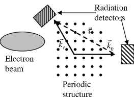
Figure 1: The two-wave diffraction geometry.

Let us perform the following simplifications: First, we shall neglect the longitudinal ($\nabla\cdot\vec{D}\to 0$) fields of the bunch, which is appropriate when the value of the Langmuir oscillation frequency $\Omega_{b}$ of the bunch is less than the values of $\Omega_{0,\tau}$. In this case, the Coulomb forces will not have an appreciable effect on electrodynamical properties of the system. Second, we shall seek for the electric field $\vec{E}$ using the method of slowly varying amplitudes. Third, we shall assume that a transversally infinite bunch executes one-dimensional motion along the $OZ$-axis (this is achieved by inducing a strong axial magnetic field in the system).

Under the conditions of two-wave diffraction, the field $\vec{E}$ can be presented as a sum

$$\vec{E}=\vec{e}_{0}E_{0}(z,t)e^{i(\vec{k}\vec{r}-\omega t)}+\vec{e}_{\tau}E_{\tau}(z,t)e^{i(\vec{k}_{\tau}\vec{r}-\omega t)},$$ (4)

where the amplitudes of the forward $E_{0}$ and diffracted $E_{\tau}$ waves are slowly varying variables. This means that for the distances comparable with the wavelength and the times comparable with the oscillation period, the values of $E_{0}$ and $E_{\tau}$ remain practically the same. Substituting (4) into (1) and (3) and then averaging them over the length $l=2j\lambda=2j\pi/k_{z}$, where $j$ is a natural number, we obtain

$$\frac{dp_{zj}}{dt}=2q_{e}e_{0z}Re\Big{(}E_{0}e^{i(k_{z}z_{j}-\omega t)}\Big{)},$$ (5)

$$\frac{1}{c}\frac{\partial E_{0}}{\partial t}+\gamma_{0}\frac{\partial E_{0}}{\partial z}+\frac{i\Omega_{0}^{2}}{2\omega c}E_{0}+\frac{i\Omega_{\tau}^{2}}{2\omega c}E_{\tau}=-\frac{2\pi}{c}\int_{z-l/2}^{z+l/2}e_{0z}j_{z}e^{i(\omega t-k_{z}z)}dz/l,$$

$$\gamma_{0}=k_{z}/k,$$

$$\frac{1}{c}\frac{\partial E_{\tau}}{\partial t}+\gamma_{\tau}\frac{\partial E_{\tau}}{\partial z}+\frac{i\Omega_{0}^{2}}{2\omega c}E_{\tau}+\frac{i\Omega_{\tau}^{2}}{2\omega c}E_{0}=-\frac{2\pi}{c}\int_{z-l/2}^{z+l/2}e_{\tau z}j_{z}e^{i(\omega t-k_{\tau z}z)}dz/l,$$

$$\gamma_{\tau}=k_{\tau z}/k.$$ (6)

Now let us complete the set of equations (5) and (2) with boundary conditions (the initial conditions are reduced to the condition that all values of the fields equal zero at $t=0$): in the plane $z=0$, let us specify the time dependence of function $f$ and set the field $E_{0}$ to zero. In the case of Bragg diffraction, the boundary condition imposed on the diffracted wave is reduced to the condition that the field $E_{\tau}$ equals zero at $z=L$, while in the case of Laue diffraction, it equals zero at $z=0$.

The difference between the two diffraction schemes is not merely kinematic, but radical. In the Bragg case, there is a synchronous wave moving against the electrons of the beam, which gives rise to the internal feedback and absolute instability. In Laue diffraction geometry, a backward wave is absent, and as a result absolute instability does not evolve. It may seem that electromagnetic radiation is not generated. However, fluctuations of the electron current (the shot noise), which always occur in real beams, are amplified when the beam enters the crystal (due to convective instability, excited in the beam).

In analyzing multiparametric problems, to which the problem of cooperative parametric (quasi-Cherenkov) radiation refers, it is convenient to write equations (5) and (2) in a dimensionless form. This procedure enabled transferring the calculation results from one set of parameters to another. The substitution of variables $\omega t\to t$, $\omega L/c\to L$, $mc\omega E_{0,\tau}/q_{e}\to E_{0,\tau}$ then gives

$$\frac{dp_{zj}}{dt}=2\theta Re\Big{(}E_{0}e^{-i(t-k_{z}z_{j}+\phi_{j})}\Big{)},$$ (7)

$$\frac{\partial E_{0}}{\partial t}+\gamma_{0}\frac{\partial E_{0}}{\partial z}+\frac{i\chi_{0}}{2}E_{0}+\frac{i\chi_{\tau}}{2}E_{\tau}=-\sum_{j}\frac{\theta\chi_{bj}}{2}\frac{e^{i(\omega t-k_{z}z_{j}+\phi_{j})}}{N_{l}},$$

$$\frac{\partial E_{\tau}}{\partial t}+\gamma_{\tau}\frac{\partial E_{\tau}}{\partial z}+\frac{i\chi_{0}}{2}E_{\tau}+\frac{i\chi_{\tau}}{2}E_{0}=0.$$ (8)

Here the quantity $\chi_{bj}=-4\pi q_{e}^{2}n_{j}/m\omega^{2}$ is determined at the moment when the $j$th particle enters the system, $n_{j}$ is the corresponding electron density, $\theta$ is the angle between the particle velocity and the wave vector $\vec{k}$, $\phi_{j}$ is the initial phase of the $j$th particle, and $N_{l}$ is the number of particles over the length $l$. The set of equations with boundary conditions contains four independent parameters: $\chi_{0,\tau}$, $\omega L/c$, $\theta$ that define the geometry of the system. In addition to these parameters, we need to specify the beam profile. Let

$$\chi_{b}=\chi_{b0}\exp(-z^{2}/L_{b}^{2}),$$ (9)

where the bunch length $L_{b}$ is further assumed to be equal to $0.1L/c$.

Obviously, in the three-diffraction case, the set of equations analogues to (2) should be rewritten as follows:

$$\frac{\partial E_{1}}{\partial t}+\gamma_{1}\frac{\partial E_{1}}{\partial z}+\frac{i\chi_{0}}{2}E_{1}+\frac{i\chi_{\tau}}{2}(E_{2}+E_{3})=-\sum_{j}\frac{\theta\chi_{bj}}{2}\frac{e^{i(t-k_{z1}z_{j}+\phi_{j})}}{N_{l}},$$

$$\frac{\partial E_{2}}{\partial t}+\gamma_{2}\frac{\partial E_{2}}{\partial z}+\frac{i\chi_{0}}{2}E_{2}+\frac{i\chi_{\tau}}{2}(E_{3}+E_{1})=0,$$

$$\frac{\partial E_{3}}{\partial t}+\gamma_{3}\frac{\partial E_{3}}{\partial z}+\frac{i\chi_{0}}{2}E_{3}+\frac{i\chi_{\tau}}{2}(E_{1}+E_{2})=0.$$ (10)

3 Simulation results

The characteristic feature of cooperative pulses is the peculiar dependence of the peak power on the number of particles $N_{b}$ in the bunch. When the particles are small in number, the radiation power monotonically increases until saturation is achieved.

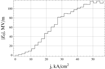
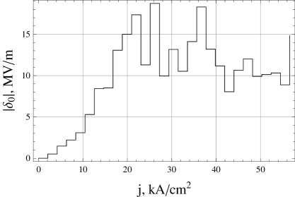
Figure 2: The Bragg case. Quasi-Cherenkov radiation at small angles to particles’ velocities: radiation amplitude (left), amplitude dispersion (right) [$\theta_{B}=67.5^{o}$, $\nu=0.1$ THz].

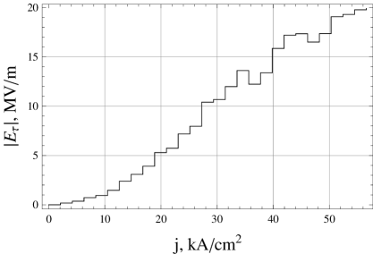
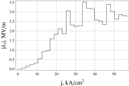
Figure 3: The Bragg case. Quasi-Cherenkov radiation at large angles to particles’ velocities: radiation amplitude (left), amplitude dispersion (right) [$\theta_{B}=67.5^{o}$, $\nu=0.1$ THz].

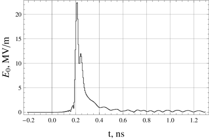
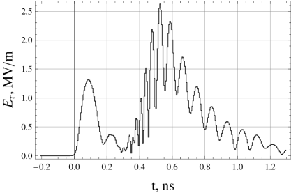
Figure 4: The Bragg case. Quasi-Cherenkov radiation at small (left) and (large) angles to particles’ velocities [$\theta_{B}=67.5^{o}$, $j=10$ kA$/$cm², $\nu=0.1$ THz].

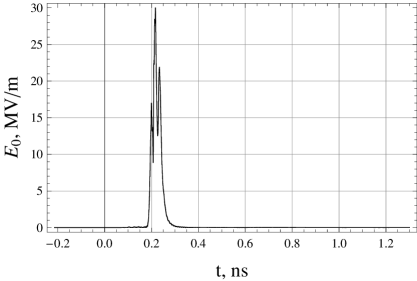
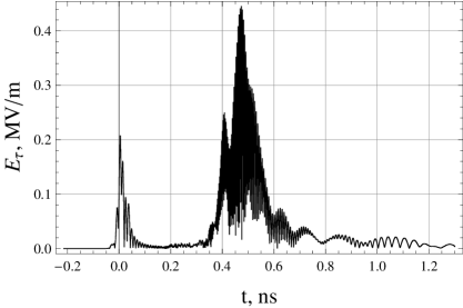
Figure 5: The Bragg case. Quasi-Cherenkov radiation at small angles to particles’ velocities: radiation amplitude (left), amplitude dispersion (right) [$\theta_{B}=67.5^{o}$, $\nu=1.0$ THz].

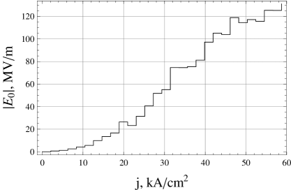
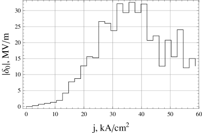
Figure 6: The Laue case. Quasi-Cherenkov radiation at small angles to particles’ velocities: radiation amplitude (left), amplitude dispersion (right) [$\theta_{B}=22.5^{o}$, $\nu=0.1$ THz].

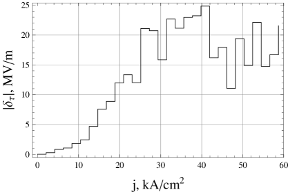
Figure 7: The Laue case. Quasi-Cherenkov radiation at large angles to particles’ velocities: radiation amplitude (left), amplitude dispersion (right) [$\theta_{B}=22.5^{o}$, $\nu=0.1$ THz].

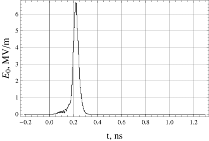
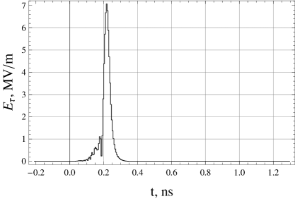
Figure 8: The Laue case. Quasi-Cherenkov radiation at small (left) and (large) angles to particles’ velocities [$\theta_{B}=22.5^{o}$, $j=10$ kA$/$cm², $\nu=0.1$ THz].

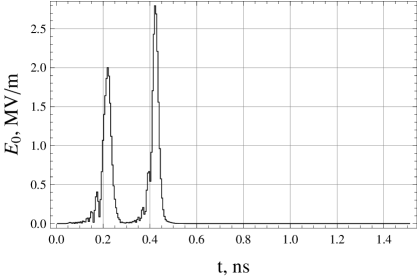
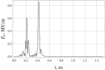
Figure 9: The Laue case. Quasi-Cherenkov radiation in the absence of shot noise [$\theta_{B}=22.5^{o}$, $L_{b}/L=1.0$, $j=10$ kA$/$cm², $\nu=0.1$ THz].

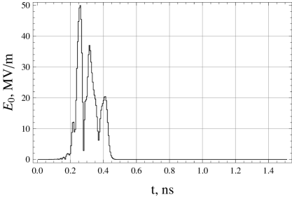
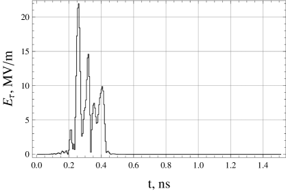
Figure 10: The Laue case. Quasi-Cherenkov radiation in the presence of shot noise [$\theta_{B}=22.5^{o}$, $L_{b}/L=1.0$, $j=10$ kA$/$cm², $\nu=0.1$ THz]

Let us see now how the dynamical diffraction of electromagnetic waves affects the cooperative radiation in crystals. How the Bragg diffraction case is different from the case of Laue diffraction?

We shall assume that $\gamma=3.0$, $\theta=0.33$ rad, $\chi_{0}/2=\chi_{\tau}=0.1$, and $L=6$ cm.

Let us start our consideration with the Bragg case. In this case, along with the electromagnetic wave emitted in the forward direction, one can observe the electromagnetic wave that is emitted by charged particles in the diffraction direction and leaves the crystal through the bunch entrance surface.

The peak radiation field emitted at small and large angles to particle velocity is investigated as a function of the peak current density $j$. The peak radiation intensity appeared to increase monotonically until saturation is achieved (Fig. 2—3). At saturation, the shot noise causes strong fluctuations in the intensity of cooperative parametric radiation. The amplitute dispersion $\delta_{0,\tau}=\sqrt{<E_{0,\tau}>^{2}-<E_{0,\tau}^{2}>}$ is presented on fig. 2 (the brackets $<..>$ denote average values).

The results of computation (Fig. 4) show that the cooperative radiation emitted at large angles lasts much longer ($t_{rad}\sim 0.6$ ns) than the particle flight time through the crystal ($t_{p}=0.2$ ns), though that is much lower than the radiation intensity emitted in forward direction. We would like to note that the long duration of parametric radiation can be observed in sponteneous processes too [4].

Figures 2—4 correspond to the frequency $\nu=0.1$ THz and current density $j=10$ kA$/$cm². If we increase $\nu$ in ten times leaving the current density unchanged the peak radiation field will be $E\approx 30$ MV$/$m which corresponds to 240 MW$/$cm² (fig. 5).

Now, let us consider the Laue case. In this case, the electromagnetic waves emitted by charged particles in the forward and diffraction directions leave the crystal through the same surface. Under Laue diffraction conditions (Fig. 6—8), the pulses of parametric radiation emitted in forward and diffracted directions have comparable amplitudes and durations.

We should point out that the shot noise results in strong fluctuations in radiation intensity at saturation. Under Laue diffraction conditions, the shot noise leads to an appreciable change in the pulse form due to the convective character of instability: in the absence of noise, the generation occurs only at the ends of the bunch of charged particles. As a result, the cooperative pulse posses a two-peak structure (Fig. 9). The presence of noise leads to an appreciable change in the pulse form: the interval between the two pulses is filled with a chaotic signal (Fig.10).

Under three-wave diffraction conditions (Fig. 11—14), the results of computation are very similar to those of the Bragg case. Namely, the intensity of cooperative radiation emitted at large angles lasts much longer than the particle flight time through the crystal, though that is much lower than the radiation intensity emitted in forward direction.

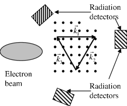
Figure 11: The three-wave diffraction geometry.

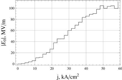
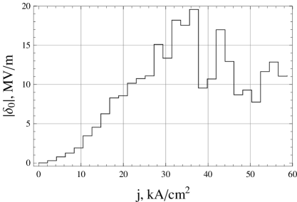
Figure 12: The three-wave diffraction case. Quasi-Cherenkov radiation at small angles to particles’ velocities: radiation amplitude (left), amplitude dispersion (right) [$\nu=0.1$ THz]

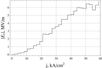
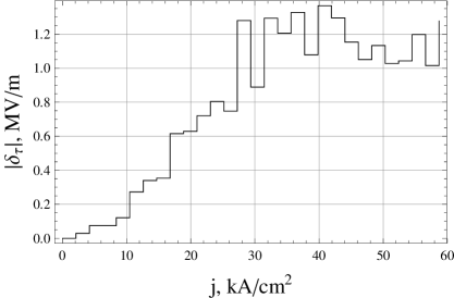
Figure 13: The three-wave diffraction case. Quasi-Cherenkov radiation at large angles to particles’ velocities: radiation amplitude (left), amplitude dispersion (right) [$\nu=0.1$ THz].

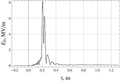
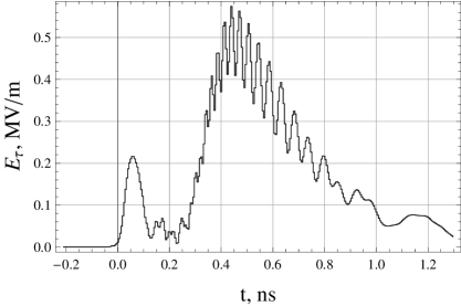
Figure 14: The three-wave diffraction case. Quasi-Cherenkov radiation at small (left) and large (right) angles to particles’ velocities [$j=10$ kA$/$cm², $\nu=0.1$ THz]

4 Conclusion

This paper studies the features of parametric (quasi-Cherenkov) cooperative radiation emitted at both large and small angles to the particle velocity direction in two- and three-wave diffraction cases. A detailed numerical analysis is given for cooperative THz radiation in artificial crystals.

The peak intensity of cooperative radiation emitted at small and large angles to particle velocity is investigated as a function of the peak current density. The peak radiation intensity appeared to increase monotonically until saturation is achieved. At saturation, the shot noise causes strong fluctuations in the intensity of cooperative parametric radiation.

It is shown that, the intensity of cooperative radiation emitted at large angles can last much longer than the particle flight time through the crystal. At saturation, the shot noise causes strong fluctuations in the intensity of cooperative parametric radiation. The intensity of THz radiation above 200 MW$/$cm² is obtained in simulations.

The complicated time structure of cooperative parametric radiation can be observed in artificial (electromagnetic, photonic) crystals in all spectral ranges (X-ray, optical, terahertz, and microwave).

It should be pointed out that thermal fluctuations become essential if $kT\geq\hbar\omega$ [19] ($k$ and $\hbar$ is the Bolzman constant and the Plank constant, respectively); namely, when $kT\gg\hbar\omega$, generation starts as a stimulated emission induced by thermal quanta rather than as a spontaneous one. This fact should be taken into account in development of terahertz generators operating at room temperature.

Appendix A Particle-in-cell method

The set of equations (5) and (2) was solved using the particle-in-cell method, which is widely used in plasma physics [13, 14]. This method implies that the solution of the kinetic equation is modeled using a large number of macroparticles moving along the characteristics of the kinetic equation. The current and charge densities are calculated from particle velocities and positions and are further used for computations of the electric field on a space-time mesh. The mesh values of the field are interpolated to the macroparticle locations; then the forces acting on macroparticles are calculated. The approach described here is close to the method described by I. J. Morey and C. K. Birdsall in [9], which was used for travelling wave tube modeling.

Let us introduce a spatial $\omega_{z}=\{z_{n}=n\Delta z,n=0,1,...,n_{max},n_{max}\Delta z=L\}$ and a time $\omega_{t}=\{t_{s}=s\Delta t,s=0,1,...\}$ mesh. Specify an implicit finite-difference scheme [15] of field equations (2) with second order accuracy in time and coordinate (the Bragg case):

$$E_{00}^{s+1}=0,E_{\tau nmax}^{s+1}=0,$$

$$0\leq n<n_{max}:$$

$$\frac{E_{\tau n+1/2}^{s+1}-E_{\tau n+1/2}^{s}}{c\Delta t}=-\gamma_{\tau}\frac{E_{\tau n+1}^{s+1/2}-E_{\tau n}^{s}}{\Delta z}-\frac{i\chi_{0}}{2}E_{\tau n}^{s+1/2}-\frac{i\chi_{\tau}}{2}E_{0n+1/2}^{s+1/2},$$

$$0<n\leq n_{max}:$$

$$\frac{E_{0n-1/2}^{s+1}-E_{0n-1/2}^{s}}{c\Delta t}=-\gamma_{0}\frac{E_{0n}^{s+1/2}-E_{0n-1}^{s+1/2}}{\Delta z}-\frac{i\chi_{0}}{2}E_{0n-1/2}^{s+1/2}$$

$$-\frac{i\chi_{\tau}}{2}E_{\tau n-1/2}^{s+1/2}-J_{0n-1/2}^{s+1/2}.$$ (11)

Let us define the source $J_{0n}^{s+1/2}$ on the right-hand side of (A), using the formula

$$J_{0n}^{s+1/2}=(J_{0n}^{s}+J_{0n}^{s+1})/2,$$

$$J_{0n}^{s+1}=\frac{2\pi\sin\theta e^{i\omega(t+\Delta t)}}{l}\Big{(}\sum_{j}Q_{j}\frac{z_{n+1}-z_{j}^{s+1}}{\Delta z}e^{-ik_{z}z_{j}^{s+1}}$$

$$+\sum_{j}Q_{j}\frac{z_{j}^{s+1}-z_{n-1}}{\Delta z}e^{-ik_{z}z_{j}^{s+1}}\Big{)}.$$ (12)

The contributions to each node come from the particles concentrated in the domain $z_{n-1}\leq z_{j}<z_{n+1}$. Summation in the first and second terms is made over all particles in the domains $z_{n}\leq z_{j}^{s+1}<z_{n+1}$ and $z_{n-1}\leq z_{j}^{s+1}<z_{n}$, respectively. The weighting factors $\frac{z_{n+1}-z_{j}^{s+1}}{\Delta z}$ and $\frac{z_{j}^{s+1}-z_{n-1}}{\Delta z}$ are responsible for linear interpolation of the contributions to the node with number $n$ that come from each particle.

Complete the leap-frog difference scheme (A) with the discrete analogues of the equations of motion of macroparticles:

$$\frac{p_{zj}^{s+1/2}-p_{zj}^{s-1/2}}{\Delta t}=2Q_{j}\theta Re\big{(}E_{0j}^{s}e^{ik_{z}z_{j}^{s+1/2}-i\omega(t+dt/2)}\big{)},$$

$$\frac{z_{j}^{s+1}-z_{j}^{s}}{\Delta t}=v_{zj}^{s+1/2},v_{zj}^{s+1/2}=\frac{p_{zj}^{s+1/2}/M_{j}}{\sqrt{1+(p_{zj}^{s+1/2}/M_{j}c)^{2}}}.$$ (13)

The field $E_{j}^{s}$ at particles’ locations can be found by means of linear interpolation from surrounding nodes:

$$E_{0j}^{s}=\frac{z_{n+1}-z_{j}^{s}}{\Delta z}E_{0n}^{s}+\frac{z_{j}^{s}-z_{n}}{\Delta z}E_{0n+1}^{s},$$

$$z_{n}\leq z_{j}^{s}<z_{n+1}.$$ (14)

Injection and extraction of particles are performed as follows: during every time step, we inject $\Delta N$ number of particles, whose initial phases are uniformly distributed on the interval $[0,\pi)$ [16]. It should be noted that the quantity $\Delta N$ obeys the Poisson statistics [17]

$$P(\Delta N)=\frac{\Delta N_{av}^{\Delta N}\exp(-\Delta N_{av})}{\Delta N!},$$ (15)

where $N_{av}$ — is an average number of particles injected during the time interval $\Delta t$.

References

- [1] R. Bonifacio, et. al. Rivista Nuovo Cimento 13 (9) (1990) 1–69.
- [2] S. D. Korovin, et. al. Phys. Rev. E74 (2006) 016501.
- [3] V. G. Baryshevsky, I. D. Feranchuk, and A. P. Ulyanenkov, Parametric X-Ray Radiation in Crystals: Theory, Experiment and Applications, Springer-Verlag, Berlin Heidelberg, 2005.
- [4] S. V.Anishchenko, V. G. Baryshevsky, and A. A. Gurinovich, Nucl. Instrum. Methods B293 (2012) 35–41.
- [5] V. G. Baryshevsky and I. D. Feranchuk. Phys. Lett. A102 (1984) 141–144.
- [6] V. G. Baryshevsky, 2012, Available from: arXiv: 1211.4769.
- [7] V.G. Baryshevsky, Vesti AN BSSR 1 (1984) 31–37.
- [8] K.A. Ispirian, Nucl. Instrum. Methods B309 (2012) 4–9.
- [9] I. J. Morey and C. K. Birdsall. Memorandum No. UCB/ERL M89/116. Electronics Research Laboratory. University of California. 1989.
- [10] T. M. Antonsen, et. al. Proceedings of the IEEE 87 (1999) 804–839.
- [11] N. S. Ginzburg, S. P. Kuznecov, and T. H. Fedoseeva, Izv. vuzov. Radiofizika 21 (1978) 1037–1052.
- [12] V. G. Baryshevsky and A. A. Gurinovich, Nucl. Instrum. Methods B252 (2006) 92–101.
- [13] J. P. Verboncoeur, Plasma Phys. Control. Fusion 47 (2005) A231–A260.
- [14] A. G. Sveshnikov and S. A. Jakunin, Matematicheskoe modelirovanie 1 (4) (1989) 1–25.
- [15] N.N. Kalitkin, Numerical methods, Nauka, Moscow, 2005.
- [16] T.M. Tran and J.S. Wurtele, Phys. Rep. 195 (1) (1990) 1–21.
- [17] B.W.J. McNeil, G.R.M. Robb, and M.W. Pole, Proc. of the PAC (2003) 950–952.
- [18] E. B. Abubakirov, A. P. Konjushkov, and A. S. Sergeev, Radiotehnika i electronika 54 (2009) 1009–1014.
- [19] S.V. Anishchenko, 2014, Available from: arXiv:1406.1483v1.