Superconducting circuit boundary conditions
beyond the Dynamical Casimir Effect

Abstract

We study analytically the time-dependent boundary conditions of superconducting microwave circuit experiments in the high plasma frequency limit, in which the conditions are Robin-type and relate the value of the field to the spatial derivative of the field. We give an explicit solution to the field evolution for boundary condition modulations that are small in magnitude but may have arbitrary time dependence, in a formalism that applies both to a semiopen waveguide and to a closed waveguide with two independently adjustable boundaries. The correspondence between the microwave Robin boundary conditions and the mechanically-moving Dirichlet boundary conditions of the Dynamical Casimir Effect is shown to break down at high field frequencies, approximately one order of magnitude above the frequencies probed in the 2011 experiment of Wilson et al. Our results bound the parameter regime in which a microwave circuit can be used to model relativistic effects in a mechanically-moving cavity, and they show that beyond this parameter regime moving mirrors produce more particles and generate more entanglement than their non-moving microwave waveguide simulations.

1 Introduction

The quantum theory of relativistic fields with moving boundaries was first explored by Moore in a remarkably original paper on the quantum formulation of linearly polarized light in a one-dimensional moving cavity [1]. The primary result of this investigation was the discovery that moving mirrors in vacuum create photons. Later, motivated by developments in quantum field theory in curved spacetimes, the specialization to a single moving mirror in Minkowski spacetime was carried out by Fulling and Davies [2], who again found that non-uniformly accelerating mirrors generate radiation. These effects, in which particles are produced by moving boundaries, are generally referred to as the Dynamical Casimir Effect (DCE) or the Nonstationary Casimir Effect [3, 4, 5].

An experimental verification of the DCE in a system with a mechanically moving boundary has remained elusive because of the technological challenges in creating sufficiently large accelerations [3, 4, 5]. However, an experimental observation of a similar particle creation effect has been reported in a mechanically static semiconductor waveguide where the boundary condition on the field is modulated electrically, by a superconducting quantum-interference device (SQUID) [6]. A related experimental observation of particle creation in Josephson metamaterial has been reported in [7]. These observations open fascinating prospects for simulating on a mechanically static desktop device quantum phenomena due to motion, including entanglement generation and degradation, in a regime where the moving system would experience significant relativistic effects [8, 9, 10].

In this paper we address the evolution of a quantum field in waveguides of the type used in the experiment of [6] in situations where the modulation of the SQUID(s) at the end(s) of the waveguide is small in magnitude but may have arbitrary time-dependence, under the further assumption that the plasma frequency of the SQUID(s) is negligibly high compared with the frequencies where the experiment operates. More precisely, recall that the field $\Phi(t,x)$ in the experiment of [6] satisfies, under the approximations described in [11, 12], the $(1+1)$-dimensional Klein-Gordon equation

$$0=\left(\frac{\partial^{2}}{\partial t^{2}}-v^{2}\frac{\partial^{2}}{\partial x^{2}}\right)\Phi(t,x)$$ (1.1)

with the boundary condition

$$0=C_{J}\ddot{\phi}(t,0)+\left(\frac{2\pi}{\Phi_{0}}\right)^{2}E_{J}(t)\Phi(t,0)+\frac{1}{L_{0}}\Phi^{\prime}(t,0)\ ,$$ (1.2)

where the cavity is at $x\leq 0$, the SQUID is at $x=0$, the meaning of the positive constants $v$, $\Phi_{0}$, $C_{J}$ and $L_{0}$ is as described in [12], and $E_{J}(t)$ can be given arbitrary time-dependence by modulating the magnetic field applied to the SQUID. In the regime where the SQUID’s plasma frequency is large compared to the frequency of $\Phi$, the time derivative term in (1.2) is negligible, and (1.2) reduces to

$$0=\Phi(t,0)+L_{0}^{\text{eff}}(t)\Phi^{\prime}(t,0)\ ,$$ (1.3)

where $L_{0}^{\text{eff}}(t)={\bigl{[}\Phi_{0}/(2\pi)\bigr{]}}^{2}{\bigl{[}L_{0}E_{J}(t)\bigr{]}}^{-1}$. We shall consider the regime in which the boundary condition (1.3) applies and the time-dependence of $L_{0}^{\text{eff}}(t)$ is arbitrary in profile but small in magnitude. The regime where the SQUID’s plasma frequency is large but not negligibly so is considered in [13, 14, 15].

Our interest in the boundary condition (1.3) is twofold. First, considering the condition in its own right, we give an explicit solution to the quantum dynamics to leading perturbative order in the time variation of the boundary condition, using a formalism that allows us to handle both the semiopen waveguide and a closed waveguide, and allowing for the closed waveguide the modulations at the two ends to remain independent of each other. The mathematical observation underlying our formalism is that (1.3) is a linear relation between the value of the field and the spatial derivative of the field, known as a Robin boundary condition, and when this condition is independent of time, it has a well-known role in making the spatial part of the wave operator in (1.1) self-adjoint and hence ensuring the unitarity of the time evolution [16, 17, 18]. A time-dependent boundary condition can then be treated perturbatively by combining the spectral methods of [16, 17, 18] to the techniques developed in [19, 20] for mechanically moving cavities. For the semiopen waveguide our results agree with those found in [21, 22, 23, 24] via a different formalism.

Second, we wish to address the sense in which (1.3) models a mechanically moving boundary of the DCE. For a Dirichlet mirror at the time-dependent location $x=x_{\text{DCE}}(t)$, the boundary condition on the field reads

$$0=\Phi\bigl{(}t,x_{\text{DCE}}(t)\bigr{)}\ .$$ (1.4)

If we choose in (1.3) $L_{0}^{\text{eff}}(t)=x_{\text{DCE}}(t)$, (1.3) reduces to (1.4) for field frequencies much smaller than $v/|L_{0}^{\text{eff}}|$, but for higher field frequencies the correspondence no longer holds. We shall see that our perturbative solution of the field evolution with the condition (1.3) indeed differs from the similar perturbative solution with the condition (1.4) for frequencies that are not much smaller than $v/|L_{0}^{\text{eff}}|$, both for a semiopen waveguide and a closed waveguide; in particular, the large frequency falloff properties of the solution are qualitatively different. Simulations of relativistic motion with the mechanically static semiconductor waveguide would hence need to take place in the low frequency regime where the successive approximations from (1.2) via (1.3) to (1.4) hold. Both the experiment of [6] and the proposals of [8, 9, 10] appear to operate within in this domain by a margin of approximately one order of magnitude.

The plan of the paper is as follows:

Section 2 considers evolution under a small discontinuous change in the boundary condition (1.3) for a semiopen waveguide, and Section 3 presents the similar analysis for the closed waveguide. Evolution under small changes in the boundary condition with arbitrary time-dependence for both types of waveguides is written out in Section 4. Section 5 compares the evolution to that under Dirichlet boundary conditions at one or two mechanically moving boundaries. Section 6 presents a summary and concluding remarks.

Appendix A collects technical identities in a perturbative expansion of Bogoliubov coefficients. Appendix B treats the evolution under the Dirichlet boundary condition at one mechanically moving boundary in a small acceleration expansion in which velocities and travel distances are unrestricted, adapting to one moving boundary the treatment of mechanically rigid cavities given in [19, 20]. In appendix C we derive the first order formula for the negativity measure of entanglement in the case when the modes have a continuous spectrum.

2 Semiopen waveguide

In this section we discuss a semiopen waveguide under a sudden change in the Robin boundary condition (1.3). Subsection 2.1 establishes the notation and reviews the known properties of a time-independent Robin boundary condition. The sudden change is implemented in subsection 2.2, and small sudden changes about the Robin boundary condition relevant for the experiment of [6] and about the Dirichlet boundary condition are discussed respectively in subsections 2.3 and 2.4.

2.1 Static boundary condition

We adopt units in which the phase velocity $v$ in (1.1) is set to unity. We may hence think of the field as a real scalar field $\phi$ on a $(1+1)$-dimensional Minkowski spacetime, with the global Minkowski coordinates $(t,x)$ and the metric $ds^{2}=-dt^{2}+dx^{2}$. We take the boundary to be at $x=0$ and the field to live in the half $0\leq x<\infty$.

We consider the massive Klein-Gordon field equation

$$(\partial_{t}^{2}-\partial_{x}^{2}+\mu^{2})\phi=0\ ,$$ (2.1)

where $\mu\geq 0$ is the mass. The massless special case $\mu=0$ reduces to (1.1). We keep here $\mu$ general, in part because setting $\mu=0$ does not significantly simplify the analysis, but also in part in view of prospective future comparisons with mechanically moving cavities in situations where transverse dimensions may generate a positive $\mu$ by Fourier decomposition [19, 20, 25].

We introduce at $x=0$ the Robin family of boundary conditions

$$0 =\phi(t,0)+D\phi^{\prime}(t,0)\ ,$$ (2.2)

where $D\in\mathbb{R}\cup\{\infty\}$ is a constant independent of $t$. The special case $D=0$ gives the Dirichlet boundary condition, $\phi(t,0)=0$, the special case $D=\infty$ gives the Neumann boundary condition, $\phi^{\prime}(t,0)=0$, and all other values of $D$ mix $\phi(t,0)$ and $\phi^{\prime}(t,0)$.

Any choice for $D$ makes $-\partial_{x}^{2}$ self-adjoint [16, 17, 18] and would hence yield a consistent quantum theory of a non-relativistic particle on the half-line, although the choice $D=0$ may in that context be considered less fine-tuned than the others [26]. In the present context of a relativistic quantum field theory, we consider only the values of $D$ that make the spectrum of $-\partial_{x}^{2}+\mu^{2}$ strictly positive. For $\mu=0$ this means $D\in(-\infty,0]\cup\{\infty\}$, and for $\mu>0$ it means $D\in(-\infty,0]\cup\{\infty\}\cup(\mu^{-1},\infty)$. A negative eigenvalue of $-\partial_{x}^{2}+\mu^{2}$ would give a tachyonic instability, and the zero eigenvalue that occurs when $\mu>0$ and $D=\mu^{-1}$ would give a zero mode and hence a theory without a Fock vacuum.

The field is quantised in the usual fashion. A continuum of mode solutions that are positive frequency with respect to $\partial_{t}$ are

$$\phi_{k}(t,x)=\frac{1}{\sqrt{\pi\omega}}\,e^{-i\omega t}\sin(kx+\delta)\ ,$$ (2.3)

where $k>0$, $\omega=\sqrt{k^{2}+\mu^{2}}$, $\delta$ is determined as a function of $k$ from

$$\tan\delta=-kD\ ,$$ (2.4)

and we may fix the phase by choosing $|\delta|<\pi/2$ for $D\in\mathbb{R}$ and $\delta=\pi/2$ for $D=\infty$. When $\mu>0$ and $\mu^{-1}<D<\infty$, there is in addition a discrete ground state mode, given by

$$\phi_{g}(t,x):=\frac{1}{{\bigl{(}\mu^{2}D^{2}-1\bigr{)}}^{1/4}}\,e^{-i\sqrt{\mu^{2}-D^{-2}}\,t}\,e^{-x/D}\ .$$ (2.5)

Writing the Klein-Gordon inner product in the conventions of [27] as

$$(\phi,\chi)=-i\int_{0}^{\infty}\bigl{(}\phi\,(\partial_{t}\overline{\chi})-(\partial_{t}\phi)\,\overline{\chi}\bigr{)}\,dx\ ,$$ (2.6)

where the overline denotes complex conjugation, the continuum modes $\phi_{k}$ are Dirac-orthonormal,

$$(\phi_{k},\phi_{k^{\prime}})=\delta(k-k^{\prime})\ ,$$ (2.7)

and when the discrete ground state $\phi_{g}$ (2.5) exists, it is normalised and orthogonal to the continuum modes. The Fock space is built on the vacuum that is annihilated by the annihilation operators associated with the continuum modes $\phi_{k}$ and with the discrete mode $\phi_{g}$ when the latter exists.

2.2 Sudden change in the boundary condition

Suppose that for $t<0$ we use the field modes as introduced above and for $t>0$ we use a similar set of field modes with $D$ replaced by $D^{\prime}$. Denoting the new continuum modes by $\tilde{\phi}_{k^{\prime}}$ and the new discrete mode by $\tilde{\phi}_{g^{\prime}}$, we may match the two sets of modes at $t=0$ in the notation of [27] as

$$\tilde{\phi}_{k^{\prime}} =\int_{0}^{\infty}\bigl{(}{{}_{\text{o}}\alpha}_{k^{\prime}k}\phi_{k}+{{}_{\text{o}}\beta}_{k^{\prime}k}\overline{\phi_{k}}\,\bigr{)}\,dk\ +{{}_{\text{o}}\alpha}_{k^{\prime}g}\phi_{g}+{{}_{\text{o}}\beta}_{k^{\prime}g}\overline{\phi_{g}}\ ,$$ (2.8a)

$$\tilde{\phi}_{g^{\prime}} =\int_{0}^{\infty}\bigl{(}{{}_{\text{o}}\alpha}_{g^{\prime}k}\phi_{k}+{{}_{\text{o}}\beta}_{g^{\prime}k}\overline{\phi_{k}}\,\bigr{)}\,dk\ +{{}_{\text{o}}\alpha}_{g^{\prime}g}\phi_{g}+{{}_{\text{o}}\beta}_{g^{\prime}g}\overline{\phi_{g}}\ ,$$ (2.8b)

where we have included the lower left subscript ${}_{\text{o}}$ in the Bogoliubov coefficients ${{}_{\text{o}}\alpha}$ and ${{}_{\text{o}}\beta}$ to indicate that the change in the boundary condition is sudden.

Expressions for the Bogoliubov coefficients can be found by taking inner products of (2.8) with the untilded modes and their complex conjugates [27]. For the continuum-to-continuum Bogoliubov coefficients, we find

$${{}_{\text{o}}\alpha}_{k^{\prime}k} =\cos(\delta-\delta^{\prime})\delta(k-k^{\prime})+\frac{\sin\delta\sin\delta^{\prime}}{\pi\sqrt{\omega\omega^{\prime}}}\left(\frac{1}{D^{\prime}}-\frac{1}{D}\right)P\left(\frac{1}{\omega-\omega^{\prime}}\right)\ ,$$ (2.9a)

$${{}_{\text{o}}\beta}_{k^{\prime}k} =\frac{\sin\delta\sin\delta^{\prime}}{\pi\sqrt{\omega\omega^{\prime}}\,(\omega+\omega^{\prime})}\left(\frac{1}{D^{\prime}}-\frac{1}{D}\right)\ ,$$ (2.9b)

where $\delta$ and $\delta^{\prime}$ are determined by

$$\tan\delta =-kD\ ,$$ (2.10a)

$$\tan\delta^{\prime} =-k^{\prime}D^{\prime}\ ,$$ (2.10b)

and $P$ in (2.9a) denotes the principal value in the integration over $k$ at $k=k^{\prime}$. In the special cases $D=0$ and $D^{\prime}=0$ the formulas (2.9) are understood in their well-defined limiting sense. The continuum-to-discrete and discrete-to-continuum Bogoliubov coefficients will not be needed below and we omit the formulas.

We note that while ${{}_{\text{o}}\beta}_{k^{\prime}k}$ (2.9b) is a function for all $k$ and $k^{\prime}$, ${{}_{\text{o}}\alpha}_{k^{\prime}k}$ (2.9a) has distributional support at $k=k^{\prime}$ because of the Dirac delta in the first term and the principal value integral in the second term.

2.3 Small sudden change: far from Dirichlet

We now consider the case where $D$ and $D^{\prime}$ are negative and close to each other. This is the situation relevant for the the waveguide experiment of [6]. (Recall that in our conventions the field $\phi$ lives at $x\geq 0$, while the field $\Phi$ in (1.1)–(1.3) lives at $x\leq 0$.)

We write

$$D =-\Lambda\ ,$$ (2.11a)

$$D^{\prime} =-\Lambda(1+\eta)\ ,$$ (2.11b)

where $\Lambda$ is a positive constant of dimension length and $\eta$ is small. The mode expansion contains no discrete mode for any value of $\mu$.

Expanding the Bogoliubov coefficients (2.9) in $\eta$, we find

$${{}_{\text{o}}\alpha}_{k^{\prime}k} =\left\{1-\frac{\eta^{2}{(k\Lambda)}^{2}}{2\,{\bigl{[}1+{(k\Lambda)}^{2}\bigr{]}}^{2}}\right\}\delta(k-k^{\prime})$$

$$\hskip 12.91663pt+\frac{\eta\Lambda kk^{\prime}}{\pi\sqrt{\omega\omega^{\prime}}\,\sqrt{1+{(k\Lambda)}^{2}}\ \sqrt{1+{(k^{\prime}\Lambda)}^{2}}}\left[1-\frac{\eta{(k^{\prime}\Lambda)}^{2}}{1+{(k^{\prime}\Lambda)}^{2}}\right]P\left(\frac{1}{\omega-\omega^{\prime}}\right)+O\bigl{(}\eta^{3}\bigr{)}\ ,$$ (2.12a)

$${{}_{\text{o}}\beta}_{k^{\prime}k} =\frac{\eta\Lambda kk^{\prime}}{\pi\sqrt{\omega\omega^{\prime}}\,(\omega+\omega^{\prime})\sqrt{1+{(k\Lambda)}^{2}}\ \sqrt{1+{(k^{\prime}\Lambda)}^{2}}}\left[1-\frac{\eta{(k^{\prime}\Lambda)}^{2}}{1+{(k^{\prime}\Lambda)}^{2}}\right]+O\bigl{(}\eta^{3}\bigr{)}\ .$$ (2.12b)

As a consistency check, we have verified that the expansion (2.12) is consistent with the identities satisfied by the Bogoliubov coefficients, collected in Appendix A, in the sense that the linear order identities (A.4a) hold and the off-diagonal part of the quadratic order identities (A.4b) holds. We are not aware of reasons to suspect inconsistencies in the diagonal part of (A.4b) but we have not undertaken the distributional analysis to examine this.

2.4 Small sudden change: near Dirichlet

As a second regime of interest, we perturb around the Dirichlet boundary condition. This case is not directly relevant for the experiment of [6], but we shall see in Section 5 that it exhibits close theoretical similarity with a mechanically moving boundary.

We set $D=0$ and assume $D^{\prime}$ to be close to $0$. If $D^{\prime}$ is negative, the result may be obtained from (2.12) by writing $\eta\Lambda=-b$ and letting $\Lambda\to 0$ while $b$ remains finite and negative but small: then $D^{\prime}=b<0$, and the Bogoliubov coefficients are given by

$${{}_{\text{o}}\alpha}_{k^{\prime}k} =\left[1-\tfrac{1}{2}{(kb)}^{2}\right]\delta(k-k^{\prime})-\frac{bkk^{\prime}}{\pi\sqrt{\omega\omega^{\prime}}}\,P\left(\frac{1}{\omega-\omega^{\prime}}\right)+O\bigl{(}{b}^{3}\bigr{)}\ ,$$ (2.13a)

$${{}_{\text{o}}\beta}_{k^{\prime}k} =-\frac{bkk^{\prime}}{\pi\sqrt{\omega\omega^{\prime}}\,(\omega+\omega^{\prime})}+O\bigl{(}b^{3}\bigr{)}\ .$$ (2.13b)

If $D^{\prime}$ is positive, the $t>0$ theory has a tachyonic instability (for all positive $D^{\prime}$ if $\mu=0$ and for $0<D^{\prime}<\mu^{-1}$ if $\mu>0$) because of the negative eigenvalue of $-\partial_{x}^{2}+\mu^{2}$; however, the tachyon is nonperturbative in $D^{\prime}$, and we have verified that just ignoring the tachyon and proceeding directly from (2.9) leads again to (2.13), where now $D^{\prime}=b>0$.

As a consistency check, we have verified that (2.13) satisfies the linear order Bogoliubov identities (A.4a) and the off-diagonal part of the quadratic order Bogoliubov identities (A.4b), regardless the sign of $b$.

3 Closed waveguide

In this section we adapt the analysis of Section 2 to a cavity waveguide that is closed at both ends. For simplicity, we treat only the massless field, $\mu=0$.

3.1 Static boundary condition

We follow the notation of Section 2, setting $\mu=0$. We place the cavity at $0\leq x\leq L$, where the positive constant $L$ is the length of the cavity.

We write the static Robin boundary conditions at the ends of the cavity as

$$0 =\phi(t,0)+D_{1}\phi^{\prime}(t,0)\ ,$$ (3.1a)

$$0 =\phi(t,L)+D_{2}\phi^{\prime}(t,L)\ ,$$ (3.1b)

where $D_{1}$ and $D_{2}$ are constants independent of $t$, taking values in $\mathbb{R}\cup\{\infty\}$.

Any choice for $D_{1}$ and $D_{2}$ makes $-\partial_{x}^{2}$ self-adjoint [16, 17, 18]. To avoid instabilities and zero modes, we assume initially $D_{1}$ and $D_{2}$ to be such that the spectrum of $-\partial_{x}^{2}$ is strictly positive. We shall however see in subsection 3.3 that a perturbative treatment in $D_{1}$ and $D_{2}$ remains consistent even in the presence of a nonperturbative tachyon, on a par with what happened for the semiopen waveguide in subsection 2.4.

The field is again quantised in the usual fashion. The Klein-Gordon inner product is as in (2.6) but integrated over $x\in[0,L]$. The equation for the eigenvalues can be written down using (3.1).

3.2 Small sudden change: far from Dirichlet

We consider the case where $D_{1}<0$ and $D_{2}>0$, and there is a sudden but small change in their values. This models a waveguide whose each end terminates at a SQUID as in the experiment of [6].

For $t<0$, we set $D_{1}=-\kappa_{1}L$ and $D_{2}=\kappa_{2}L$, where $\kappa_{1}$ and $\kappa_{2}$ are positive dimensionless constants. With this boundary condition $-\partial_{x}^{2}$ is positive definite. The mode functions are

$$\phi_{q}(t,x)=\sqrt{\frac{(1+\kappa_{1}^{2}q^{2})(1+\kappa_{2}^{2}q^{2})}{qF(q)}}\,e^{-iqt/L}\sin(qx/L+\delta_{q}),$$ (3.2)

where

$$F(q):=(1+\kappa_{1}+\kappa_{1}^{2}q^{2})(1+\kappa_{2}+\kappa_{2}^{2}q^{2})-\kappa_{1}\kappa_{2}\ ,$$ (3.3)

$q$ goes over the positive solutions to

$$\cot q=\frac{\kappa_{1}\kappa_{2}q^{2}-1}{(\kappa_{1}+\kappa_{2})q}\ ,$$ (3.4)

$\tan\delta_{q}=\kappa_{1}q$, and we choose the phase so that $0<\delta_{q}<\pi/2$. There is exactly one $q$ in each interval $m\pi<q<(m+1)\pi$, $m=0,1,2,\ldots$. The mode functions are normalised to $(\phi_{q},\phi_{q}^{\prime})=\delta_{qq^{\prime}}$.

For $t>0$, we set $D_{1}=(-\kappa_{1}+\eta_{1})L$ and $D_{2}=(\kappa_{2}+\eta_{2})L$, where $\eta_{1}$ and $\eta_{2}$ are dimensionless constants, assumed to be small. We work perturbatively in $\eta_{1}$ and $\eta_{2}$, setting both of them to be proportional to a formal expansion parameter $\eta$ which at the end is set to unity. The mode functions are proportional to $e^{-ikt}\sin(kx+\delta)$ where $k$ and $\delta$ are determined from (3.1). We label the mode functions by the positive solutions to

$$\cot p=\frac{\kappa_{1}\kappa_{2}p^{2}-1}{(\kappa_{1}+\kappa_{2})p}\ ,$$ (3.5)

such that $k=p/L+O(\eta)$, we denote them by $\tilde{\phi}_{p}$, and we choose their phase to agree with that of (3.2) in the zeroth perturbative order. We then find that the eigenfrequencies are given by

$$k_{p}=\left(1+\frac{\eta_{1}(1+\kappa_{2}^{2}p^{2})-\eta_{2}(1+\kappa_{1}^{2}p^{2})}{F(p)}\right)\frac{p}{L}\ \ +O\bigl{(}\eta^{2}\bigr{)}\ .$$ (3.6)

The Bogoliubov coefficients are now defined by matching the modes at $t=0$ as

$$\tilde{\phi}_{p}=\sum_{q}\bigl{(}{{}_{\text{o}}\alpha}_{pq}\phi_{q}+{{}_{\text{o}}\beta}_{pq}\overline{\phi_{q}}\,\bigr{)}\ .$$ (3.7)

Proceeding as in [19, 25], we find

$${{}_{\text{o}}\alpha}_{pp} =1+O\bigl{(}\eta^{2}\bigr{)}\ ,$$ (3.8a)

$${{}_{\text{o}}\alpha}_{pq} =\frac{\Bigl{[}\eta_{1}\sqrt{(1+\kappa_{2}^{2}p^{2})(1+\kappa_{2}^{2}q^{2})}-{(-1)}^{\varphi_{p}+\varphi_{q}}\eta_{2}\sqrt{(1+\kappa_{1}^{2}p^{2})(1+\kappa_{1}^{2}q^{2})}\,\Bigr{]}\sqrt{pq}}{(p-q)\sqrt{F(p)F(q)}}$$

$$\hskip 12.91663pt+O\bigl{(}\eta^{2}\bigr{)}\ \ \ \text{for $p\neq q$}\ ,$$ (3.8b)

$${{}_{\text{o}}\beta}_{pq} =-\frac{\Bigl{[}\eta_{1}\sqrt{(1+\kappa_{2}^{2}p^{2})(1+\kappa_{2}^{2}q^{2})}-{(-1)}^{\varphi_{p}+\varphi_{q}}\eta_{2}\sqrt{(1+\kappa_{1}^{2}p^{2})(1+\kappa_{1}^{2}q^{2})}\,\Bigr{]}\sqrt{pq}}{(p+q)\sqrt{F(p)F(q)}}$$

$$\hskip 12.91663pt+O\bigl{(}\eta^{2}\bigr{)}\ ,$$ (3.8c)

where the map $q\mapsto\varphi_{q}$ labels the consecutive solutions to (3.4) by consecutive integers. The expressions for the order $\eta^{2}$ terms in (3.6) and (3.8) are lengthy and we suppress them here.

As a consistency check, the linear terms in (3.8) satisfy the linear order Bogoliubov identities (A.4a). We are not aware of reasons to suspect inconsistencies in the quadratic order identities (A.4b) but examining these would require a nontrivial evaluation of the left-hand side in (A.4b) and we have not carried out this evaluation.

3.3 Small sudden change: near Dirichlet

We consider also a perturbation around the Dirichlet boundary condition. If $\eta_{1}<0$ and $\eta_{2}>0$, the result may be obtained from (3.8) simply by taking the limit $\kappa_{1}\to 0$ and $\kappa_{2}\to 0$. The $t<0$ mode functions are given by

$$\phi_{n}(t,x)=\frac{1}{\sqrt{\pi n}}\,e^{-in\pi t/L}\sin(n\pi x/L)\ ,$$ (3.9)

where $n=1,2,\ldots$. Using positive integers to label both the $t<0$ mode functions and the $t>0$ mode functions, we find that the $t>0$ eigenfrequencies are given by

$$k_{m}=\left(1+(\eta_{1}-\eta_{2})+{(\eta_{1}-\eta_{2})}^{2}\right)\frac{\pi m}{L}\ \ +O\bigl{(}\eta^{3}\bigr{)}\ ,$$ (3.10)

where $m=1,2,\ldots$, and the Bogoliubov coefficients are given by

$${{}_{\text{o}}\alpha}_{mm} =1-\tfrac{1}{6}\bigl{(}\eta_{1}^{2}+\eta_{1}\eta_{2}+\eta_{2}^{2}\bigr{)}\,m^{2}\pi^{2}+O\bigl{(}\eta^{3}\bigr{)}\ ,$$ (3.11a)

$${{}_{\text{o}}\alpha}_{mn} =\frac{\bigl{(}\eta_{1}-{(-1)}^{m+n}\eta_{2}\bigr{)}\sqrt{mn}}{(m-n)}$$

$$\hskip 12.91663pt-\frac{\bigl{(}\eta_{1}-{(-1)}^{m+n}\eta_{2}\bigr{)}(\eta_{1}-\eta_{2})\,n\sqrt{mn}}{{(m-n)}^{2}}+O\bigl{(}\eta^{3}\bigr{)}\ \ \ \text{for $m\neq n$}\ ,$$ (3.11b)

$${{}_{\text{o}}\beta}_{mn} =-\frac{\bigl{(}\eta_{1}-{(-1)}^{m+n}\eta_{2}\bigr{)}\sqrt{mn}}{(m+n)}$$

$$\hskip 12.91663pt-\frac{\bigl{(}\eta_{1}-{(-1)}^{m+n}\eta_{2}\bigr{)}(\eta_{1}-\eta_{2})\,n\sqrt{mn}}{{(m+n)}^{2}}+O\bigl{(}\eta^{3}\bigr{)}\ ,$$ (3.11c)

where we have now displayed also the order $\eta^{2}$ terms. If $\eta_{1}\geq 0$ and/or $\eta_{2}\leq 0$, the $t>0$ theory may have tachyonic instabilities or zero modes; however, both of these are nonperturbative, and we have verified that setting $D_{1}=D_{2}=0$ for $t<0$, $D_{1}=\eta_{1}L$ and $D_{2}=\eta_{2}L$ for $t>0$, ignoring any tachyons or zero modes, and working directly from (3.1) and (3.7), yields (3.10) and (3.11) regardless the signs of $\eta_{1}$ and $\eta_{2}$.

As a consistency check, the expressions in (3.11) can be verified to satisfy the perturbative Bogoliubov identities (A.4). The elements of the matrix square on the left-hand side of (A.4a) are given by absolutely convergent sums that can be evaluated by residue techniques.

4 Boundary condition with arbitrary time-dependence

When the boundary condition has arbitrary time dependence but the variations remain so small in magnitude that first-order perturbation theory suffices, the evolution of the field can be obtained by composing the sudden changes of Sections 2 and 3 and passing to the limit [20]. We discuss first the semiopen waveguide and then the closed waveguide.

4.1 Semiopen waveguide

For the semiopen waveguide of Section 2, we consider a boundary condition of the form (2.2) where $D$ may change in time but only within the interval $t_{0}\leq t\leq t_{f}$.

4.1.1 Far from Dirichlet

Consider first the far-from Dirichlet case. We write $D=-\Lambda\bigl{(}1+\eta(t)\bigr{)}$, where $\Lambda$ is a positive constant and the function $\eta(t)$ is vanishing outside the interval $t_{0}\leq t\leq t_{f}$ and satisfies $|\eta(t)|\ll 1$.

At $t<t_{0}$, we introduce early time basis modes that are as in (2.3) but with the replacement $e^{-i\omega t}\to e^{-i\omega(t-t_{0})}$. At $t>t_{f}$, we similarly introduce late time basis modes that are as in (2.3) but with the replacement $e^{-i\omega t}\to e^{-i\omega(t-t_{f})}$. Let $\alpha_{k^{\prime}k}$ and $\beta_{k^{\prime}k}$ be the coefficients in the Bogoliubov transformation from the early time modes to the late time modes. Working perturbatively in $\eta$, we may proceed as in [20], and the outcome can be read off from formulas (6) and (7) therein. We find

$$\alpha_{k^{\prime}k} =e^{i\omega^{\prime}(t_{f}-t_{0})}\left(\delta(k-k^{\prime})+\hat{A}_{k^{\prime}k}+O\bigl{(}\eta^{2}\bigr{)}\right)\ ,$$ (4.1a)

$$\beta_{k^{\prime}k} =e^{i\omega^{\prime}(t_{f}-t_{0})}\hat{B}_{k^{\prime}k}+O\bigl{(}\eta^{2}\bigr{)}\ ,$$ (4.1b)

where

$$\hat{A}_{k^{\prime}k} =-\frac{i\Lambda kk^{\prime}}{\pi\sqrt{\omega\omega^{\prime}}\,\sqrt{1+{(k\Lambda)}^{2}}\ \sqrt{1+{(k^{\prime}\Lambda)}^{2}}}\int_{t_{0}}^{t_{f}}e^{-i(\omega^{\prime}-\omega)(t-t_{0})}\,\eta(t)\,dt\ ,$$ (4.2a)

$$\hat{B}_{k^{\prime}k} =\frac{i\Lambda kk^{\prime}}{\pi\sqrt{\omega\omega^{\prime}}\,\sqrt{1+{(k\Lambda)}^{2}}\ \sqrt{1+{(k^{\prime}\Lambda)}^{2}}}\int_{t_{0}}^{t_{f}}e^{-i(\omega^{\prime}+\omega)(t-t_{0})}\,\eta(t)\,dt\ .$$ (4.2b)

When $\mu=0$, (4.1) and (4.2) reduce to what was found in [21, 22, 23, 24] via a different formalism.

4.1.2 Near Dirichlet

In the near-Dirichlet case, we take $D=b(t)$, where the function $b(t)$ is vanishing outside the interval $t_{0}\leq t\leq t_{f}$. Proceeding as above, we find

$$\alpha_{k^{\prime}k} =e^{i\omega^{\prime}(t_{f}-t_{0})}\left(\delta(k-k^{\prime})+\hat{A}_{k^{\prime}k}+O\bigl{(}b^{2}\bigr{)}\right)\ ,$$ (4.3a)

$$\beta_{k^{\prime}k} =e^{i\omega^{\prime}(t_{f}-t_{0})}\hat{B}_{k^{\prime}k}+O\bigl{(}b^{2}\bigr{)}\ ,$$ (4.3b)

where

$$\hat{A}_{k^{\prime}k} =\frac{ikk^{\prime}}{\pi\sqrt{\omega\omega^{\prime}}}\int_{t_{0}}^{t_{f}}e^{-i(\omega^{\prime}-\omega)(t-t_{0})}\,b(t)\,dt\ ,$$ (4.4a)

$$\hat{B}_{k^{\prime}k} =-\frac{ikk^{\prime}}{\pi\sqrt{\omega\omega^{\prime}}}\int_{t_{0}}^{t_{f}}e^{-i(\omega^{\prime}+\omega)(t-t_{0})}\,b(t)\,dt\ .$$ (4.4b)

4.2 Closed waveguide

For the closed waveguide of Section 3, we consider a boundary condition of the form (3.1) where $D_{1}$ and $D_{2}$ may change in time but only within the interval $t_{0}\leq t\leq t_{f}$. We may proceed as above. The only new aspect is that the method of [20] needs to be generalised to accommodate the linear term that appears in the frequencies (3.6) and (3.10).

4.2.1 Far from Dirichlet

In the far-from Dirichlet case, we write $D_{1}=\bigl{(}-\kappa_{1}+\eta_{1}(t)\bigr{)}L$ and $D_{2}=\bigl{(}\kappa_{2}+\eta_{2}(t)\bigr{)}L$, where $\kappa_{1}$ and $\kappa_{2}$ are positive constants and the functions $\eta_{1}(t)$ and $\eta_{2}(t)$ are vanishing outside the interval $t_{0}\leq t\leq t_{f}$ and satisfy $|\eta_{1}(t)|\ll 1$ and $|\eta_{2}(t)|\ll 1$. Indexing the mode functions in the notation of subsection (3.2), writing

$$\omega_{p}=p/L\ ,\ \ \ \omega_{q}=q/L\ ,$$ (4.5)

and proceeding as above, we find that the coefficients in the Bogoliubov transformation from the early time modes to the late time modes are given by

$$\alpha_{pq} =e^{i\omega_{p}(t_{f}-t_{0})}\left(\delta_{pq}+\hat{A}_{pq}+O\bigl{(}\eta^{2}\bigr{)}\right)\ ,$$ (4.6a)

$$\beta_{pq} =e^{i\omega_{p}(t_{f}-t_{0})}\hat{B}_{pq}+O\bigl{(}\eta^{2}\bigr{)}\ ,$$ (4.6b)

where

$$\hat{A}_{pq} =\frac{i\sqrt{pq}}{L\sqrt{F(p)F(q)}}\left[\sqrt{(1+\kappa_{2}^{2}p^{2})(1+\kappa_{2}^{2}q^{2})}\int_{t_{0}}^{t_{f}}e^{-i(\omega_{p}-\omega_{q})(t-t_{0})}\,\eta_{1}(t)\,dt\right.$$

$$\hskip 30.1388pt\left.-{(-1)}^{\varphi_{p}+\varphi_{q}}\sqrt{(1+\kappa_{1}^{2}p^{2})(1+\kappa_{1}^{2}q^{2})}\int_{t_{0}}^{t_{f}}e^{-i(\omega_{p}-\omega_{q})(t-t_{0})}\,\eta_{2}(t)\,dt\right]\ ,$$ (4.7a)

$$\hat{B}_{pq} =-\frac{i\sqrt{pq}}{L\sqrt{F(p)F(q)}}\left[\sqrt{(1+\kappa_{2}^{2}p^{2})(1+\kappa_{2}^{2}q^{2})}\int_{t_{0}}^{t_{f}}e^{-i(\omega_{p}+\omega_{q})(t-t_{0})}\,\eta_{1}(t)\,dt\right.$$

$$\hskip 30.1388pt\left.-{(-1)}^{\varphi_{p}+\varphi_{q}}\sqrt{(1+\kappa_{1}^{2}p^{2})(1+\kappa_{1}^{2}q^{2})}\int_{t_{0}}^{t_{f}}e^{-i(\omega_{p}+\omega_{q})(t-t_{0})}\,\eta_{2}(t)\,dt\right]\ .$$ (4.7b)

4.2.2 Near Dirichlet

In the near-Dirichlet case, we write $D_{1}=\eta_{1}(t)L$ and $D_{2}=\eta_{2}(t)L$. Indexing the past and future mode functions by positive integers in the notation of subsection (3.3), and writing

$$\omega_{m}=\pi m/L\ ,\ \ \ \omega_{n}=\pi n/L\ ,$$ (4.8)

we find

$$\alpha_{mn} =e^{i\omega_{m}(t_{f}-t_{0})}\left(\delta_{mn}+\hat{A}_{mn}+O\bigl{(}\eta^{2}\bigr{)}\right)\ ,$$ (4.9a)

$$\beta_{mn} =e^{i\omega_{m}(t_{f}-t_{0})}\hat{B}_{mn}+O\bigl{(}\eta^{2}\bigr{)}\ ,$$ (4.9b)

where

$$\hat{A}_{mn} =\frac{i\pi\sqrt{mn}}{L}\int_{t_{0}}^{t_{f}}e^{-i(\omega_{m}-\omega_{n})(t-t_{0})}\,\bigl{(}\eta_{1}(t)-{(-1)}^{m+n}\eta_{2}(t)\bigr{)}\,dt\ ,$$ (4.10a)

$$\hat{B}_{mn} =-\frac{i\pi\sqrt{mn}}{L}\int_{t_{0}}^{t_{f}}e^{-i(\omega_{m}+\omega_{n})(t-t_{0})}\,\bigl{(}\eta_{1}(t)-{(-1)}^{m+n}\eta_{2}(t)\bigr{)}\,dt\ .$$ (4.10b)

5 Comparison

We are now ready to compare the evolution under the time-dependent Robin boundary condition to the evolution under the Dirichlet condition at a mechanically moving boundary.

5.1 Semiopen waveguide

For the semiopen waveguide, the evolution of a field with mass $\mu\geq 0$ under the time-dependent Robin boundary condition was given in subsection 4.1. The evolution of a massless field under a Dirichlet condition at a mechanically moving boundary is given in Appendix B in terms of the acceleration of the boundary, in a small acceleration approximation that allows the velocity and the travel distance to remain arbitrary and overlaps with the DCE literature results [3, 4, 5] in the common domain of validity.

Comparing (4.3)–(4.4) and (B.11)–(B.12), we see that the massless field with the mechanically moving boundary can be simulated to the leading order in perturbation theory by the $\mu=0$ near-Dirichlet Robin boundary condition provided we choose $b(t)$ so that $a(\tau)=\partial_{\tau}^{2}b(\tau)$, where $a(\tau)$ is the proper acceleration of the boundary as a function of its proper time $\tau$, and the modulation starts and ends so gently that both $b$ and $\dot{b}$ vanish. This is precisely the relation one would have expected from the low frequency equivalence between the Robin boundary condition (1.3) and the mechanically moving Dirichlet boundary condition (1.4). The simulation is reliable in the frequency range where the first-order perturbation theory results on both the Robin side and on the mechanical side remain reliable; we shall not attempt to quantify this range more precisely, but for given $a(\tau)$ and $b(\tau)$ the range is unlikely to include arbitrarily high frequencies.

Comparing further (4.3)–(4.4) and (B.11)–(B.12) with (4.1)–(4.2), we see that the massless field with the mechanically moving boundary can be simulated by the $\mu=0$ far-from-Dirichlet Robin boundary condition provided we choose $\eta(t)$ so that $a(\tau)=-\Lambda\partial_{\tau}^{2}\eta(\tau)$, the frequencies are much smaller than $\Lambda^{-1}$, and the modulation starts and ends so gently that both $\eta$ and $\dot{\eta}$ vanish. Again, this is precisely the outcome one would have expected from (1.3) and (1.4). When the frequencies are not much smaller than $\Lambda^{-1}$, the evolution with the Robin boundary condition differs from the evolution with the mechanically moving boundary because the square root factors in (4.2) differ from unity.

Investigating these differences further, recall that the beta coefficients are directly related to the total photon production number by:

$$N=\int{|\beta_{k^{\prime}k}|}^{2}\,dk\,dk^{\prime}\ .$$ (5.1)

Taking $\eta(t)$ to be a sinusoidal function:

$$\eta(t)=\varepsilon\sin[\omega_{d}(t-t_{0})]\ ,$$ (5.2)

with positive constant $\varepsilon\ll 1$ and driving frequency $\omega_{d}$, the integrals in (4.2) can be performed exactly. The dominant part of the photon flux occurs for frequencies below the driving frequency. We therefore define the photon flux density, $n(\overline{k})$, as a function of the reduced frequency $\overline{k}:=k^{\prime}/\omega_{d}$, by

$$n(\overline{k}):=\omega_{d}\int_{0}^{\infty}{|\beta_{\omega_{d}\overline{k}\;k}|}^{2}\,dk\ ,$$ (5.3)

so that

$$N=\int_{0}^{\infty}n(\overline{k})\,d\overline{k}\ .$$ (5.4)

Figure 1 presents numerical plots of the photon flux density for $\Lambda\ll 1/\omega_{d}$ and $\Lambda\gg 1/\omega_{d}$. In both cases the spectrum has in the range $0<\overline{k}<1$ a distinctive parabolic shape that is qualitatively characteristic of the DCE, and for $\Lambda\ll 1/\omega_{d}$ there is good agreement with the zero temperature curve of Figure 8 in [12].

For a quantitative comparison with the DCE, Figure 1 presents also the photon flux density for the mechanically moving Dirichlet boundary, obtained from (B.11)–(B.12) with the matching $a(\tau)=-\Lambda\partial_{\tau}^{2}\eta(\tau)$. When the effective length, $\Lambda$, is much smaller than the effective wavelength of the driving frequency ($\Lambda\ll 1/\omega_{d}$), the moving boundary and Robin-boundary systems produce almost identical spectral functions, even though the modulation used for the plot has nonvanishing $\dot{\eta}$ at the start and end. On the other hand, when the effective length is larger than the effective wavelength of the driving frequency ($\Lambda\gg 1/\omega_{d}$), the spectral functions from the moving boundary system and the Robin-boundary systems differ: the radiation from the moving boundary has a higher intensity, and the spectrum from the Robin boundary condition decays more rapidly at high frequencies. Both of these behaviours result from the square root factors which suppress the beta coefficients in (4.2).

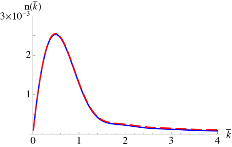
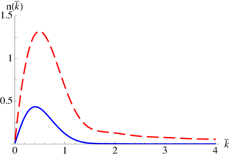
Figure 1: Photon flux densities $n(\overline{k})$ (5.3) for the semiopen waveguide in terms of the reduced frequency $\overline{k}=k/\omega_{d}$ for moving boundary (red dashed) and non-moving time-varying Robin boundary (blue solid). (Left) In the small effective length limit $\Lambda\ll 1/\omega_{d}$ the two systems display near identical behavior. (Right) In the large effective length limit $\Lambda\gg 1/\omega_{d}$ the moving and non-moving systems have different photon production profiles. In both plots we use the values (in units with $v=1$), $\epsilon=0.25$, $\omega_{d}=0.155$mm^-1 and $t_{f}-t_{0}=40.5$mm. In the Left plot we take $\Lambda=0.44$mm and in the Right plot we take $\Lambda=10$mm. The parameters in the Left plot can be matched to those suggested in [12] by taking the propagation velocity $v=1.2\times 10^{11}$mm/s and noting that $L^{\text{eff}}_{0}\rightarrow\Lambda$, $\delta L^{\text{eff}}_{0}/L^{\text{eff}}_{0}\rightarrow\varepsilon$.

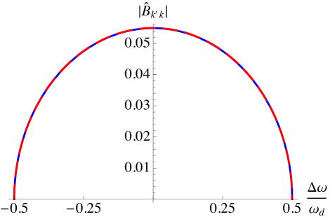
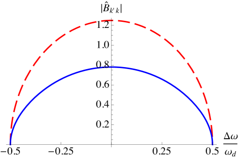
Figure 2: The plots show the negativity function $|\hat{B}_{k^{\prime}k}|=\mathcal{N}/\Delta k$ (see appendix C) with $k=\omega_{d}/2+\Delta\omega$ and $k^{\prime}=\omega_{d}/2-\Delta\omega$ in terms of $\Delta\omega/\omega_{d}$ for moving boundary (red dashed) and non-moving time-varying Robin boundary (blue solid). (Left) In the small effective length limit $\Lambda\ll 1/\omega_{d}$ the two systems display near identical behavior. (Right) In the large effective length limit $\Lambda\gg 1/\omega_{d}$ the moving system produces more entanglement than the non-moving system. We use the same parameters as in Fig. 1.

One of the signatures of the DCE radiation is that emitted photons are entangled. We can quantify the amount of entanglement produced using the negativity [28, 29] which is defined as minus the sum of the negative eigenvalues of the partially transposed state. We show in appendix C that for perturbative Bogoliubov coefficients of the type (4.1)–(4.2) the leading term in the negativity between sharply peaked field modes $k$ and $k^{\prime}$ is given by $\Delta k|\hat{B}_{k^{\prime}k}|$ where $\Delta k$ is the spectral line-width of the frequencies.

For the driving function given in equation (5.2), $|\hat{B}_{k^{\prime}k}|$ is highest for values of $k+k^{\prime}$ near the driving frequency. Therefore, we define $\Delta\omega=(k-k^{\prime})/2$, and we expand the frequencies near half driving-frequency as:

$$k =\omega_{d}/2+\Delta\omega\ ,$$ (5.5a)

$$k^{\prime} =\omega_{d}/2-\Delta\omega\ .$$ (5.5b)

The results for $|\hat{B}_{k^{\prime}k}|$ as a function of $\Delta\omega/\omega_{d}$ are shown in Fig. 2. These plots are qualitatively similar to those of Fig. 14 in [12] for the “without resonator” line. We again observe good agreement when $\Lambda\ll 1/\omega_{d}$ between moving mirrors and non-moving microwave waveguides. Also, when $\Lambda\gg 1/\omega_{d}$ we find that the moving mirrors generate more entanglement than their associated non-moving microwave waveguide simulations.

The entanglement considered above is entanglement between the field modes. This entanglement could be observed directly with a homodyne setup by coupling the emitted radiation into an optics circuit with stationary photodetectors. Another possibility would be to harvest the entanglement by inserting localised detectors, such as an atomic qubit. This has been discussed in a range of settings in [30, 31, 32, 33, 34, 35] and the references therein.

5.2 Closed waveguide

For the closed waveguide, the evolution of a massless field under the time-dependent Robin boundary condition was given in subsection 4.2. The evolution of a massless field in a moving, mechanically rigid cavity of proper length $L$ with Dirichlet boundary conditions is given by [19, 20]

$$\alpha_{mn} =e^{i\omega_{m}(\tau_{f}-\tau_{0})}\left(\delta_{mn}+\hat{A}_{mn}+O\bigl{(}a^{2}\bigr{)}\right)\ ,$$ (5.6a)

$$\beta_{mn} =e^{i\omega_{m}(\tau_{f}-\tau_{0})}\hat{B}_{mn}+O\bigl{(}a^{2}\bigr{)}\ ,$$ (5.6b)

where

$$\hat{A}_{nn} =0\ ,$$ (5.7a)

$$\hat{A}_{mn} =-\frac{i\pi\sqrt{mn}\bigl{(}1-{(-1)}^{m+n}\bigr{)}}{L^{2}{(\omega_{m}-\omega_{n})}^{2}}\,\int_{\tau_{0}}^{\tau_{f}}e^{-i(\omega_{m}-\omega_{n})(\tau-\tau_{0})}\,a(\tau)\,d\tau\ \ \ \text{for $m\neq n$}\ ,$$ (5.7b)

$$\hat{B}_{mn} =\frac{i\pi\sqrt{mn}\bigl{(}1-{(-1)}^{m+n}\bigr{)}}{L^{2}{(\omega_{m}+\omega_{n})}^{2}}\,\int_{\tau_{0}}^{\tau_{f}}e^{-i(\omega_{m}+\omega_{n})(\tau-\tau_{0})}\,a(\tau)\,d\tau\ ,$$ (5.7c)

$m$ and $n$ are positive integers, $\omega_{m}$ and $\omega_{n}$ are given by (4.8), $\tau$ is the proper time at the centre of the cavity and $a(\tau)$ is the proper acceleration at the centre of the cavity.

Comparing (4.9)–(4.10) and (5.6)–(5.7), we see that the massless field in the rigidly moving cavity can be simulated to the leading order in perturbation theory by the near-Dirichlet Robin boundary condition provided we choose $\eta_{1}(\tau)=\eta_{2}(\tau)$ and $a(\tau)=L\partial_{\tau}^{2}\eta_{1}(\tau)$, and the modulation starts and ends so gently that both $\eta$ and $\dot{\eta}$ vanish. Again, this is precisely the relation one would have expected from (1.3) and (1.4), and the simulation is reliable in the frequency range where the first-order perturbation theory results on both sides are reliable.

Comparing further with (4.6)–(4.7), we see that the rigidly moving cavity can be simulated by the far-from-Dirichlet Robin boundary condition with $\eta_{1}(\tau)=\eta_{2}(\tau)$ and $a(\tau)=L\partial_{\tau}^{2}\eta_{1}(\tau)$ when the frequencies are much smaller than $\kappa_{1}^{-1}$ and $\kappa_{2}^{-1}$ and the modulation starts and ends so gently that both $\eta$ and $\dot{\eta}$ vanish.

We anticipate that the simulation can be extended to a moving cavity that is not rigid, in the small amplitude regime commonly considered in the DCE literature [3, 4, 5], by equating $L\eta_{1}(t)$ (respectively $L\eta_{2}(t)$) to the variation in the position of the left (right) boundary. We have however not examined this question systematically.

6 Conclusions

In this paper we have analysed the evolution of a quantum field in $1+1$ dimensions under time-dependent Robin boundary conditions that occur in superconducting microwave circuit experiments in the high plasma frequency limit. We solved the evolution explicitly to linear order in the time variation of the Robin boundary condition, in a formalism that allowed us to handle both a semiopen waveguide and a closed waveguide, and for the latter allowing the boundary conditions at the two ends to be varied independently. For frequencies that are much smaller than the effective inverse length associated with the SQUID(s) at the end(s) of the waveguide, we verified that a suitable modulation of the SQUID(s) allows the waveguide to simulate a Dirichlet boundary condition at a mechanically moving boundary of the DCE, even in the regime where the mechanical motion is relativistic; both the experiment reported in [6] and the experimental proposals of [8, 9, 10] appear to operate within in this domain by a margin of approximately one order of magnitude. For higher frequencies the waveguide still exhibits particle creation and mode mixing, but these can no longer be quantitatively matched to those of the DCE, and in particular the large frequency falloff properties in the evolution are qualitatively different. These features in the large frequency Bogoliubov coefficients result in differing particle emission spectrum for the moving and non-moving systems when the effective length is larger than the inverse driving frequency $L\gg 1/\omega_{d}$. In this limit, mechanically moving boundary radiation can be characterised as having a larger total flux and a less steep falloff at high frequencies compared to radiation from the static waveguide with time-varying Robin boundary conditions.

While the analogy between a moving Dirichlet boundary and a time-varying Robin boundary condition is useful for simulation purposes it is important to keep in mind that the physical systems corresponding to these two situations are different and therefore can lead to different outcomes. On the one hand, our results support proposals to simulate in a mechanically static waveguide quantum phenomena due to motion, including entanglement generation and degradation, even in a regime where the mechanically moving system experiences significant relativistic effects [8, 9, 10]. On the other hand, our results demonstrate that the interpretation of a waveguide experiment in terms of the simulation of the DCE is possible only in certain parameter ranges. Within the Robin boundary condition approximation that we have analysed, the range of DCE interpretation is determined just by the effective inverse length scale set by the SQUID(s) at the end(s) of the waveguide. It remains a subject to future work to establish the range of DCE interpretation when all relevant effects beyond the Robin boundary condition approximation are considered [11, 12], including the effects due to a large but finite SQUID plasma frequency analysed in [13, 14, 15].

Appendix A Perturbative Bogoliubov identities

In this appendix we record identities satisfied by a perturbative expansion of the Bogoliubov coefficients. These identities are used in the main text for consistency checks of the perturbative treatment.

Let $\alpha$ and $\beta$ denote the matrices of a Bogoliubov transformation in the notation of [27], with the matrix elements $\alpha_{jk}$ and $\beta_{jk}$. The indices may be discrete or continuous; in the latter case the matrix is understood as the kernel of an integral operator and may include a distributional part. By construction, the matrices satisfy the Bogoliubov identities

$$\mathbb{I} =\alpha\alpha^{\dagger}-\beta\beta^{\dagger}\ ,$$ (A.1a)

$$0 =\alpha\beta^{T}-\beta\alpha^{T}\ ,$$ (A.1b)

where $\mathbb{I}$ stands for the identity matrix.

Suppose now that $\alpha$ and $\beta$ have the formal power series expansions

$$\alpha =\mathbb{I}+\epsilon\alpha_{1}+\epsilon^{2}\alpha_{2}+\epsilon^{3}\alpha_{3}+\cdots\ ,$$ (A.2a)

$$\beta =\epsilon\beta_{1}+\epsilon^{2}\beta_{2}+\epsilon^{3}\beta_{3}+\cdots\ ,$$ (A.2b)

where $\epsilon$ is a real-valued expansion parameter. Substituting (A.2) in (A.1) and collecting terms order by order, order $\epsilon^{0}$ is identically satisfied while orders $\epsilon^{1}$ and $\epsilon^{2}$ give

$$\epsilon^{1}: \ \ \begin{cases}0=\alpha_{1}+\alpha_{1}^{\dagger}\ ,\\ 0=\beta_{1}-\beta_{1}^{T}\ ,\end{cases}$$ (A.3a)

$$\epsilon^{2}: \ \ \begin{cases}0=\alpha_{1}\alpha_{1}^{\dagger}-\beta_{1}\beta_{1}^{\dagger}+\alpha_{2}+\alpha_{2}^{\dagger}\ ,\\ 0=\beta_{1}\alpha_{1}^{T}-\alpha_{1}\beta_{1}^{T}+\beta_{2}-\beta_{2}^{T}\ .\end{cases}$$ (A.3b)

When $\alpha$ and $\beta$ are real, (A.3) simplifies to

$$\epsilon^{1}: \ \ \begin{cases}\alpha_{1}=-\alpha_{1}^{T}\ ,\\ \beta_{1}=\beta_{1}^{T}\ ,\end{cases}$$ (A.4a)

$$\epsilon^{2}: \ \ {(\alpha_{1}\pm\beta_{1})}^{2}=\alpha_{2}+\alpha_{2}^{T}\pm\bigl{(}\beta_{2}-\beta_{2}^{T}\bigr{)}\ .$$ (A.4b)

Appendix B Accelerated boundary in Minkowski spacetime

In this appendix we consider a quantised massless scalar field in $(1+1)$-dimensional Minkowski spacetime subject to the Dirichlet boundary condition at one accelerated boundary, in the limit where the acceleration is treated perturbatively but may have arbitrary time-dependence, and the velocity and travel distance of the boundary remain arbitrary. We follow the methods that were developed for a mechanically rigid accelerated cavity in [19, 20]. The results overlap with those in the DCE literature [3, 4, 5] for small amplitude oscillations in the common domain of validity. The corresponding problem for a classical scalar field has been analysed in [36, 37, 38].

B.1 Inertial boundary to uniformly accelerated boundary

We work with a massless scalar field $\phi$ in $(1+1)$-dimensional Minkowski spacetime, in the notation of the main text: the metric is $ds^{2}=-dt^{2}+dx^{2}$, and the wave equation is (2.1) with $\mu=0$.

For $t<0$, we take the field to live in the half-space $x\geq a^{-1}$, where $a$ is a positive constant of dimension inverse length, and we adopt at $x=a^{-1}$ the Dirichlet boundary condition. We adopt the basis of mode functions

$$\phi_{k}(t,x)=\frac{1}{\sqrt{\pi k}}\,e^{-ikt}\sin[k(x-a^{-1})]\ ,$$ (B.1)

where $k>0$. $\phi_{k}$ has the positive frequency $k$ with respect to $\partial_{t}$, and the normalisation in the Klein-Gordon inner product is $(\phi_{k},\phi_{k^{\prime}})=\delta(k-k^{\prime})$.

For $t\geq 0$, we make the boundary follow the uniformly-accelerated worldline $x=\sqrt{t^{2}+a^{-2}}$. The proper acceleration of the boundary is equal to $a$. The field lives in the region $x\geq\sqrt{t^{2}+a^{-2}}$, and we take the field to satisfy the Dirichlet boundary condition at the accelerated boundary. We adopt the basis of mode functions

$$\Phi_{k}(t,x)=\frac{1}{2i\,\sqrt{\pi k}}\left\{\bigl{[}a(x-t)\bigr{]}^{ik/a}-\bigl{[}a(x+t)\bigr{]}^{-ik/a}\right\}\ ,$$ (B.2)

where $k>0$. $\Phi_{k}$ has the positive frequency $k/a$ with respect to the boost Killing vector $x\partial_{t}+t\partial_{x}$, and it has the positive frequency $k$ with respect to the proper time of the boundary. The normalisation in the Klein-Gordon inner product is $(\Phi_{k},\Phi_{k^{\prime}})=\delta(k-k^{\prime})$.

At the junction $t=0$, we match the two sets of modes by the Bogoliubov transformation

$$\Phi_{k^{\prime}} =\int_{0}^{\infty}\bigl{(}{{}_{\text{o}}\alpha}_{k^{\prime}k}\phi_{k}+{{}_{\text{o}}\beta}_{k^{\prime}k}\overline{\phi_{k}}\,\bigr{)}\,dk\ .$$ (B.3)

From the inner products that give the Bogoliubov coefficients [27], we find

$${{}_{\text{o}}\alpha}_{k^{\prime}k} =\frac{1}{\pi a}\sqrt{\frac{k^{\prime}}{k}}\,\operatorname{Re}\left[\int_{1}^{\infty}\frac{dy}{y}\,y^{-ik^{\prime}/a}\,e^{i(k/a)(y-1)}\right]\ ,$$ (B.4a)

$${{}_{\text{o}}\beta}_{k^{\prime}k} =\frac{1}{\pi a}\sqrt{\frac{k^{\prime}}{k}}\,\operatorname{Re}\left[\int_{1}^{\infty}\frac{dy}{y}\,y^{ik^{\prime}/a}\,e^{i(k/a)(y-1)}\right]\ .$$ (B.4b)

B.2 Small acceleration expansion

We wish to find the asymptotic form of ${{}_{\text{o}}\alpha}_{k^{\prime}k}$ and ${{}_{\text{o}}\beta}_{k^{\prime}k}$ (B.4) when the acceleration $a$ of the boundary is small compared with both $k$ and $k^{\prime}$.

The small $a$ expansion of ${{}_{\text{o}}\beta}_{k^{\prime}k}$ may be obtained by applying to (B.4b) the method of repeated integration by parts [39]. The result is

$${{}_{\text{o}}\beta}_{kk^{\prime}} =\frac{a\,\sqrt{k^{\prime}k}}{\pi{(k+k^{\prime})}^{3}}+O\bigl{(}a^{3}\bigr{)}\ .$$ (B.5)

The small $a$ expansion of ${{}_{\text{o}}\alpha}_{k^{\prime}k}$ is more involved since we expect the coefficients in this expansion to be no longer functions but distributions, the leading term being $\delta(k-k^{\prime})$. We shall not give a rigorous treatment but proceed heuristically as follows.

Starting from the integral in (B.4a), we replace $k$ in the integrand by $k+i\epsilon$ where $\epsilon>0$. If $\epsilon$ is considered fixed, the asymptotic small $a$ expansion can be obtained by the method of repeated integration by parts [39], with the result

$${{}_{\text{o}}\alpha}_{k^{\prime}k} =\frac{1}{\pi}\sqrt{\frac{k^{\prime}}{k}}\left\{-\operatorname{Im}\left[\frac{1}{{(k-k^{\prime}+i\epsilon)}}\right]+a\operatorname{Re}\left[\frac{k+i\epsilon}{{(k-k^{\prime}+i\epsilon)}^{3}}\right]\vphantom{\left[\frac{(k+i\epsilon)\bigl{[}2(k+i\epsilon)+k^{\prime}\bigr{]}}{{(k-k^{\prime}+i\epsilon)}^{4}}\right]}\right.$$

$$\hskip 51.6665pt+\left.a^{2}\operatorname{Im}\left[\frac{(k+i\epsilon)\bigl{[}2(k+i\epsilon)+k^{\prime}\bigr{]}}{{(k-k^{\prime}+i\epsilon)}^{5}}\right]+O\bigl{(}a^{3}\bigr{)}\right\}\ .$$ (B.6)

Each of the three terms shown in (B.6) has a well-defined distributional limit as $\epsilon\to 0$, as follows from the identity

$$\lim_{\epsilon\to 0^{+}}\int dk\,\frac{f(k)}{k+i\epsilon}=-i\pi f(0)+P\int dk\,\frac{f(k)}{k}\ ,$$ (B.7)

and its derivatives. Assuming that the $\epsilon\to 0$ limit commutes with the small $a$ expansion, we obtain

$${{}_{\text{o}}\alpha}_{k^{\prime}k} =\delta(k-k^{\prime})+aG_{1}(k^{\prime},k)+a^{2}G_{2}(k^{\prime},k)+O\bigl{(}a^{3}\bigr{)}\ ,$$ (B.8)

where the distributions $G_{1}$ and $G_{2}$ are given by

$$\int_{0}^{\infty}dk\,G_{1}(k^{\prime},k)\,f(k) =\frac{{(k^{\prime})}^{1/2}}{2\pi}P\int_{0}^{\infty}dk\,\frac{1}{{(k-k^{\prime})}}\,\partial_{k}^{2}\left(k^{1/2}\,f(k)\right)\ ,$$ (B.9a)

$$\int_{0}^{\infty}dk\,G_{2}(k^{\prime},k)\,f(k) =-\frac{{(k^{\prime})}^{1/2}}{12}\,\partial^{4}_{k^{\prime}}\left({(k^{\prime})}^{3/2}f(k^{\prime})\right)-\frac{{(k^{\prime})}^{3/2}}{24}\,\partial^{4}_{k^{\prime}}\left({(k^{\prime})}^{1/2}f(k^{\prime})\right)\ .$$ (B.9b)

Both $G_{1}$ and $G_{2}$ are hence representable by a function except at the coincidence limit, and we may write

$$G_{1}(k^{\prime},k) =\frac{\sqrt{kk^{\prime}}}{\pi\,{(k-k^{\prime})}^{3}} \text{for $k\neq k^{\prime}$}\ ,$$ (B.10a)

$$G_{2}(k^{\prime},k) =0 \text{for $k\neq k^{\prime}$}\ .$$ (B.10b)

As a consistency check, the expansions in (B.5) and (B.8) satisfy the linear order Bogoliubov identities (A.4a). The quadratic order Bogoliubov identities (A.4b) would require a distributional treatment and we shall not analyse them here.

B.3 Arbitrarily-accelerated boundary

Let $\tau$ denote the proper time of the boundary and $a(\tau)$ the proper acceleration of the boundary, such that positive (negative) values of $a(\tau)$ mean acceleration towards increasing (decreasing) $x$. We assume that $a(\tau)$ is vanishing outside the interval $\tau_{0}\leq\tau\leq\tau_{f}$ and non-negative within this interval, and we assume that $a(\tau)$ remains much smaller than the frequencies to be considered.

We define the early (respectively late) time modes by (B.1) in the inertial frame in which the boundary is at rest in the early (late) times. Proceeding as in [19, 20], or in Section 4 of the present paper, we find that the Bogoliubov coefficients from the early time modes to the late time modes are

$$\alpha_{k^{\prime}k} =e^{ik^{\prime}(\tau_{f}-\tau_{0})}\left(\delta(k-k^{\prime})+\hat{A}_{k^{\prime}k}+O\bigl{(}a^{2}\bigr{)}\right)\ ,$$ (B.11a)

$$\beta_{k^{\prime}k} =e^{ik^{\prime}(\tau_{f}-\tau_{0})}\hat{B}_{k^{\prime}k}+O\bigl{(}a^{2}\bigr{)}\ ,$$ (B.11b)

where

$$\hat{A}_{k^{\prime}k} =-\frac{i\sqrt{kk^{\prime}}}{\pi{(k-k^{\prime})}^{2}}\,\int_{\tau_{0}}^{\tau_{f}}e^{-i(k^{\prime}-k)(\tau-\tau_{0})}\,a(\tau)\,d\tau\ \ \ \text{for $k\neq k^{\prime}$}\ ,$$ (B.12a)

$$\hat{B}_{k^{\prime}k} =\frac{i\sqrt{kk^{\prime}}}{\pi{(k+k^{\prime})}^{2}}\,\int_{\tau_{0}}^{\tau_{f}}e^{-i(k^{\prime}+k)(\tau-\tau_{0})}\,a(\tau)\,d\tau\ ,$$ (B.12b)

and we omit the examination of the distributional part of $\hat{A}_{k^{\prime}k}$ at $k=k^{\prime}$.

The above treatment assumes $a(\tau)$ to be non-negative. We shall not examine the validity of (B.12) when $a(\tau)$ may take negative values.

Appendix C Entanglement formula for continuous spectra

In this appendix we derive the formula for the perturbative approximation to the bipartite mode entanglement of the field, as measured by the entanglement negativity, in the case when the field solutions have continuous spectra. These generalise the negativity formulas found for field solutions with discrete eigenvalues in [40]. The field is prepared initially in the vacuum state and is subjected to an evolution which can be described by Bogoliubov transformations that are assumed to take the general form:

$$\alpha_{k^{\prime}k} =c(k^{\prime})\left(\delta(k-k^{\prime})+\hat{A}_{k^{\prime}k}+O\bigl{(}\eta^{2}\bigr{)}\right)\ ,$$ (C.1a)

$$\beta_{k^{\prime}k} =c(k^{\prime})\hat{B}_{k^{\prime}k}+O\bigl{(}\eta^{2}\bigr{)}\ ,$$ (C.1b)

where $\eta\ll 1$, $k$ and $k^{\prime}$ are continuous real-valued parameters, $\hat{A}_{k^{\prime}k}$ and $\hat{B}_{k^{\prime}k}$ are of linear order in $\eta$ and $c(k)$ is a phase taking the general form, $c(k)=e^{if(k)}$, where $f$ is a real-valued function of $k$. Furthermore, we assume that $\hat{A}_{k^{\prime}k}$ and $\hat{B}_{k^{\prime}k}$ satisfy the conditions:

$$\hat{A}_{k^{\prime}k} = -\hat{A}_{kk^{\prime}}^{\star}\ \ \ \text{for $k\neq k^{\prime}$},$$ (C.2a)

$$\hat{B}_{k^{\prime}k} = \hat{B}_{kk^{\prime}},$$ (C.2b)

where the star denotes complex conjugation. Equations (C.2) are satisfied by the evolution in the semiopen waveguide (4.1) and by the evolution with the accelerated mirror (B.12).

The added difficulty of systems with continuous spectra is that the states are Dirac $\delta$-normalised which can lead to apparent infinities in formulas for the entanglement if not correctly handled. The infinities are an artefact of working with infinitely precise frequencies which in practice is not possible — there is always a spectral line-width, $\Delta k$, associated with the measurement of a frequency. Experiments which measure bipartite entanglement of the field do so by measuring two distinct frequencies each with a small line-width. For simplicity, we will assume that the modes measured are uniform wavepackets of frequencies having spectral line-width $\Delta k$ and central frequencies $k_{\text{p}}$, $k_{\text{p}}^{\prime}$ respectively. We define:

$$f_{k_{\text{p}}}(k)=\begin{cases}\frac{1}{\sqrt{\Delta k}}&\text{for $k\in(k_{\text{p}}-\frac{\Delta k}{2},k_{\text{p}}+\frac{\Delta k}{2})$},\\[4.30554pt] 0&\text{otherwise.}\end{cases}$$ (C.3)

We will also assume that the measured frequencies are sufficiently separated such that there is no overlap of their supports in frequency space:

$$\int f_{k_{\text{p}}}(k)f_{k_{\text{p}}^{\prime}}(k)dk=0.$$ (C.4)

Let $\hat{a}(k)$ be the annihilation operator associated with the frequency $k$. After the evolution the annihilation operators are transformed by the Bogoliubov transfomations according to:

$$\hat{\bar{a}}(k)=\int\left(\alpha_{kk^{\prime}}^{\star}\hat{a}(k^{\prime})-\beta_{kk^{\prime}}^{\star}\hat{a}(k^{\prime})^{\dagger}\right)dk^{\prime}.$$ (C.5)

The quadrature operators associated with these frequencies are:

$$\hat{\bar{x}}(k) = \hat{\bar{a}}(k)+\hat{\bar{a}}(k)^{\dagger},$$ (C.6a)

$$\hat{\bar{p}}(k^{\prime}) = \frac{1}{i}\left(\hat{\bar{a}}(k)-\hat{\bar{a}}(k)^{\dagger}\right),$$ (C.6b)

where we use the conventions of [41].

As already alluded these frequencies are not measured precisely rather the actual measurement occurs over a small band of frequencies. We can define the quadrature operators associated with a wavepacket centred at the frequency $k_{\text{p}}$ by:

$$\hat{\bar{x}}_{k_{\text{p}}} = \int f_{k_{\text{p}}}(k)\hat{\bar{x}}(k)dk,$$ (C.7a)

$$\hat{\bar{p}}_{k_{\text{p}}} = \int f_{k_{\text{p}}}(k)\hat{\bar{p}}(k)dk.$$ (C.7b)

A short calculation shows that the quadrature operators satisfy the commutation relations:

$$\left[\hat{\bar{x}}_{i},\hat{\bar{p}}_{j}\right] = 2i\delta_{ij},$$ (C.8a)

$$\left[\hat{\bar{x}}_{i},\hat{\bar{x}}_{j}\right] = \left[\hat{\bar{p}}_{i},\hat{\bar{p}}_{j}\right]=0,$$ (C.8b)

where $i,j\in\{k_{\text{p}},k_{\text{p}}^{\prime}\}$.

Since the Bogoliubov transformations are linear and the vacuum state is a Gaussian state, it follows that the final state of the field will also be a Gaussian state. Gaussian states are completely characterised by their first and second statistical moments. It is the second moments which are important for determining the amount of entanglement in a Gaussian state. The second moments can be arranged into a covariance matrix: we define $R=(\hat{\bar{x}}_{k_{\text{p}}},\hat{\bar{p}}_{k_{\text{p}}},\hat{\bar{x}}_{k_{\text{p}}^{\prime}},\hat{\bar{p}}_{k_{\text{p}}^{\prime}})$, then the covariance matrix can be defined by:

$$\sigma_{ij}=\frac{1}{2}\langle\{R_{i},R_{j}\}\rangle-\langle R_{i}\rangle\langle R_{j}\rangle,$$ (C.9)

where curly braces denote anti-commutator and the covariance matrix is normalised such that the covariance matrix of the vacuum state is the identity matrix. Expectation values are to be taken with respect to the initial state which in our case is the vacuum state. It is easy to see that the second term in (C.9) vanishes.

We define the kernels:

$$X(k,k^{\prime}) = \frac{1}{2}\langle\{\hat{\bar{x}}(k),\hat{\bar{x}}(k^{\prime})\}\rangle$$ (C.10a)

$$= \int dl(\alpha_{kl}^{\star}-\beta_{kl})(\alpha_{k^{\prime}l}-\beta_{k^{\prime}l}^{\star}),$$

$$H(k,k^{\prime}) = \frac{1}{2}\langle\{\hat{\bar{x}}(k),\hat{\bar{p}}(k^{\prime})\}\rangle$$ (C.10b)

$$= i\int dl(\alpha_{kl}^{\star}-\beta_{kl})(\alpha_{k^{\prime}l}+\beta_{k^{\prime}l}^{\star})-i\delta(k-k^{\prime}),$$

$$P(k,k^{\prime}) = \frac{1}{2}\langle\{\hat{\bar{p}}(k),\hat{\bar{p}}(k^{\prime})\}\rangle$$ (C.10c)

$$= \int dl(\alpha_{kl}^{\star}+\beta_{kl})(\alpha_{k^{\prime}l}+\beta_{k^{\prime}l}^{\star}),$$

and the matrix:

$$S(k,k^{\prime})=\left(\begin{array}[]{cc}X(k,k^{\prime})&H(k,k^{\prime})\\ H(k^{\prime},k)&P(k,k^{\prime})\end{array}\right),$$ (C.13)

then the covariance matrix takes the form:

$$\sigma=\left(\begin{array}[]{cc}\sigma_{a}&\sigma_{c}\\ \sigma_{c}^{T}&\sigma_{b}\end{array}\right),$$ (C.16)

where superscript $T$ indicates matrix transposition and

$$\sigma_{a} \equiv \int f_{k_{\text{p}}}(k)f_{k_{\text{p}}}(k^{\prime})S(k,k^{\prime})dkdk^{\prime},$$ (C.17a)

$$\sigma_{b} \equiv \int f_{k_{\text{p}}^{\prime}}(k)f_{k_{\text{p}}^{\prime}}(k^{\prime})S(k,k^{\prime})dkdk^{\prime},$$ (C.17b)

$$\sigma_{c} \equiv \int f_{k_{\text{p}}}(k)f_{k_{\text{p}}^{\prime}}(k^{\prime})S(k,k^{\prime})dkdk^{\prime}.$$ (C.17c)

Using relations (C.1) and (C.2), the matrix $S(k,k^{\prime})$ simplifies to

$$S(k,k^{\prime})=\delta(k-k^{\prime})+S^{1}(k,k^{\prime})+\mathcal{O}(\eta^{2}),$$ (C.18)

where the matrix elements of $S^{1}(k,k^{\prime})$ are given by:

$$S^{1}_{11}=-S^{1}_{22} = -c(k)^{\star}\beta_{k^{\prime}k}^{\star}-c(k^{\prime})\beta_{kk^{\prime}},$$ (C.19a)

$$S^{1}_{21}=-S^{1}_{12} = i\big{(}c(k)^{\star}\beta_{k^{\prime}k}^{\star}-c(k^{\prime})\beta_{kk^{\prime}}\big{)}.$$ (C.19b)

We can also write the covariance matrix as a Taylor expansion in $\eta$:

$$\sigma=\sigma^{0}+\sigma^{1}+\mathcal{O}(\eta^{2}),$$ (C.20)

and with equation (C.18) it is easily seen that $\sigma^{0}$ is the $4\times 4$ identity matrix.

To determine the bipartite entanglement, it is necessary to calculate the symplectic eigenvalues, $\tilde{\nu}_{\pm}$, of the covariance matrix of the partially transposed state, $\tilde{\sigma}$. The partial transpose is implemented by a transformation of the covariance matrix given by [42]:

$$\sigma_{a} \rightarrow \tilde{\sigma}_{a}=\sigma_{a},$$ (C.21a)

$$\sigma_{b} \rightarrow \tilde{\sigma}_{b}=\sigma_{3}\sigma_{b}\sigma_{3},$$ (C.21b)

$$\sigma_{c} \rightarrow \tilde{\sigma}_{c}=\sigma_{c}\sigma_{3},$$ (C.21c)

where $\sigma_{3}=\text{diag}(1,-1)$ is the $z$-direction Pauli matrix.

The symplectic values of $\tilde{\sigma}$ can be found from the absolute values of the eigenvalues of the matrix $\Omega\tilde{\sigma}$, where $\Omega=\text{diag}(\omega,\omega)$ and

$$\omega=\left(\begin{array}[]{cc}0&1\\ -1&0\end{array}\right).$$ (C.24)

The zeroth order eigenvalues are $\pm i$ and both eigenvalues have double degeneracy. It is therefore necessary to use degenerate perturbation theory to determine the eigenvalues to the linear order. The linear order corrections to the eigenvalues are found to be:

$$\lambda_{\pm}=\pm 2i\sqrt{I},$$ (C.25)

where

$$I\equiv\int dl\int dl^{\prime}\int dk\int dk^{\prime}f_{k_{\text{p}}}(l)f_{k_{\text{p}}^{\prime}}(l^{\prime})f_{k_{\text{p}}}(k)f_{k_{\text{p}}^{\prime}}(k^{\prime})c(l^{\prime})c(k)^{\star}\beta_{ll^{\prime}}\beta_{k^{\prime}k}^{\star}.$$ (C.26)

The symplectic eigenvalues are therefore:

$$\tilde{\nu}_{\pm}=|1\pm 2\sqrt{I}|,$$ (C.27)

and the negativity is:

$$\mathcal{N}=\text{max}\left(0,\frac{1-\tilde{\nu}_{s}}{2\tilde{\nu}_{s}}\right),$$ (C.28)

where $\tilde{\nu}_{s}$ is the smallest of the two symplectic values. Let us now assume that the wavepackets are very sharply peaked $\Delta k/k_{\text{p}}\ll 1$ and $\Delta k/k_{\text{p}}^{\prime}\ll 1$, then the integrals in equation (C.26) can be approximated by:

$$I = \Delta k^{2}c(k_{\text{p}}^{\prime})c(k_{\text{p}})^{\star}\beta_{k_{\text{p}}k_{\text{p}}^{\prime}}\beta_{k_{\text{p}}^{\prime}k_{\text{p}}}^{\star}$$ (C.29)

$$= \Delta k^{2}|\hat{B}_{k_{\text{p}}k_{\text{p}}^{\prime}}|^{2},$$

and the negativity (to first order in $\eta$) simplifies to:

$$\mathcal{N}=\Delta k|\hat{B}_{k_{\text{p}}k_{\text{p}}^{\prime}}|.$$ (C.30)

This is the continuous spectrum formula for the entanglement negativity and holds for non-integer values of the frequencies. It is equivalent to the formula for discrete frequency modes in the case when the modes have opposite parity, i.e., when $(k+k^{\prime})$ is odd [40].

References

- [1] G. T. Moore, “Quantum Theory of the Electromagnetic Field in a Variable Length One Dimensional Cavity,” J. Math. Phys. 11, 2679 (1970).
- [2] S. A. Fulling and P. C. W. Davies, “Radiation from a Moving Mirror in Two Dimensional Space-Time: Conformal Anomaly,” Proc. R. Soc. London, Ser. A 348, 393 (1976).
- [3] V. V. Dodonov, “Nonstationary Casimir effect and analytical solutions for quantum fields in cavities with moving boundaries,” Adv. Chem. Phys. 119, 309 (2001) [quant-ph/0106081].
- [4] V. V. Dodonov, “Current status of the dynamical Casimir effect,” Phys. Scripta 82, 038105 (2010).
- [5] D. A. R. Dalvit, P. A. Maia Neto and F. D. Mazzitelli, “Fluctuations, dissipation and the dynamical Casimir effect,” Lect. Notes Phys. 834, 419 (2011) [arXiv:1006.4790 [quant-ph]].
- [6] C. M. Wilson, G. Johansson, A. Pourkabirian, M. Simoen, J. R. Johansson, T. Duty, F. Nori and P. Delsing, “Observation of the dynamical Casimir effect in a superconducting circuit,” Nature 479, 376 (2011) [arXiv:1105.4714 [quant-ph]].
- [7] P. Lähteenmäki, G. S. Paraoanu, J. Hassel and P. J. Hakonen, “Dynamical Casimir effect in a Josephson metamaterial,” Proc. Nat. Acad. Sci. 110, 4234 (2013) [arXiv:1111.5608 [cond-mat.mes-hall]].
- [8] N. Friis, A. R. Lee, K. Truong, C. Sabín, E. Solano, G. Johansson and I. Fuentes, “Relativistic Quantum Teleportation with Superconducting Circuits,” Phys. Rev. Lett. 110, 113602 (2013) [arXiv:1211.5563 [quant-ph]].
- [9] J. Lindkvist, C. Sabín, I. Fuentes, A. Dragan, I.-M. Svensson, P. Delsing and G. Johansson, “Twin paradox with macroscopic clocks in superconducting circuits,” Phys. Rev. A 90, 052113 (2014) [arXiv:1401.0129 [quant-ph]].
- [10] J. Lindkvist, C. Sabín, G. Johansson and I. Fuentes, “Motion and gravity effects in the precision of quantum clocks,” arXiv:1409.4235 [quant-ph].
- [11] J. R. Johansson, G. Johansson, C. M. Wilson and F. Nori, “Dynamical Casimir Effect in a Superconducting Coplanar Waveguide,” Phys. Rev. Lett. 103, 147003 (2009) [arXiv:0906.3127 [cond-mat.supr-con]].
- [12] J. R. Johansson, G. Johansson, C. M. Wilson and F. Nori, “Dynamical Casimir effect in superconducting microwave circuits,” Phys. Rev. A 82, 052509 (2010).
- [13] W. Wustmann and V. Shumeiko, “Parametric resonance in tunable superconducting cavities,” Phys. Rev. B 87, 184501 (2013) [arXiv:1302.3484 [cond-mat.mes-hall]].
- [14] C. D. Fosco, F. C. Lombardo and F. D. Mazzitelli, “Vacuum fluctuations and generalized boundary conditions,” Phys. Rev. D 87, 105008 (2013) [arXiv:1303.6176 [hep-th]].
- [15] S. Felicetti, M. Sanz, L. Lamata, G. Romero, G. Johansson, P. Delsing and E. Solano, “Dynamical Casimir Effect Entangles Artificial Atoms,” Phys. Rev. Lett. 113, 093602 (2014) [arXiv:1402.4451 [quant-ph]].
- [16] M. Reed and B. Simon, Methods of Modern Mathematical Physics II: Fourier Analysis, Self-adjointness (Academic, New York, 1975).
- [17] J. Blank, P. Exner and M. Havlíček, Hilbert Space Operators in Quantum Physics, 2nd edition (Springer, New York, 2008).
- [18] G. Bonneau, J. Faraut and G. Valent, “Selfadjoint extensions of operators and the teaching of quantum mechanics,” Am. J. Phys. 69, 322 (2001) [arXiv:quant-ph/0103153].
- [19] D. E. Bruschi, I. Fuentes and J. Louko, “Voyage to Alpha Centauri: Entanglement degradation of cavity modes due to motion,” Phys. Rev. D 85, 061701 (2012) [arXiv:1105.1875 [quant-ph]].
- [20] D. E. Bruschi, J. Louko, D. Faccio and I. Fuentes, “Mode-mixing quantum gates and entanglement without particle creation in periodically accelerated cavities,” New J. Phys. 15, 073052 (2013) [arXiv:1210.6772 [quant-ph]].
- [21] H. O. Silva and C. Farina, “A simple model for the dynamical Casimir effect for a static mirror with time-dependent properties,” Phys. Rev. D 84, 045003 (2011) [arXiv:1102.2238 [hep-th]].
- [22] C. Farina, H. O. Silva, A. L. C. Rego and D. T. Alves, “Time-dependent Robin boundary conditions in the dynamical Casimir effect,” Int. J. Mod. Phys. Conf. Ser. 14, 306 (2012) [arXiv:1201.3846 [quant-ph]].
- [23] A. L. C. Rego, J. P. d. S. Alves, D. T. Alves and C. Farina, “Relativistic bands in the spectrum of created particles via the dynamical Casimir effect,” Phys. Rev. A 88, 032515 (2013) [arXiv:1309.3159 [quant-ph]].
- [24] A. L. C. Rego, C. Farina, H. O. Silva and D. T. Alves, “New signatures of the dynamical Casimir effect in a superconducting circuit,” Phys. Rev. D 90, 025003 (2014) [arXiv:1405.3720 [quant-ph]].
- [25] N. Friis, A. R. Lee and J. Louko, “Scalar, spinor, and photon fields under relativistic cavity motion,” Phys. Rev. D 88, 064028 (2013) [arXiv:1307.1631 [quant-ph]].
- [26] B. Belchev and M. A. Walton, “Robin boundary conditions and the Morse potential in quantum mechanics”, J. Phys. A 43, 085301 (2010) [arXiv:1002.2139 [quant-ph]].
- [27] N. D. Birrell and P. C. W. Davies, Quantum Fields in Curved Space (Cambridge University Press, 1982).
- [28] A. Peres, “Separability Criterion for Density Matrices,” Phys. Rev. Lett. 77, 1413 (1996) [arXiv:quant-ph/9604005].
- [29] M. Horodecki, P. Horodecki and R. Horodecki, “Separability of mixed states: necessary and sufficient conditions,” Phys. Lett. A 223, 1 (1996) [arXiv:quant-ph/9605038].
- [30] G. Benenti, S. Siccardi and G. Strini, “Exotic states in the dynamical Casimir effect,” Eur. Phys. J. D 68, 139 (2014) [arXiv:1312.6315 [quant-ph]].
- [31] G. Benenti, A. D’Arrigo, S. Siccardi and G. Strini, “Dynamical Casimir effect in quantum-information processing,” Phys. Rev. A 90, 052313 (2014) [arXiv:1407.7567 [quant-ph]].
- [32] G. Benenti and G. Strini, “Dynamical Casimir effect and minimal temperature in quantum thermodynamics,” arXiv:1412.4819 [quant-ph].
- [33] J. Doukas and L. C. L. Hollenberg, “Loss of spin entanglement for accelerated electrons in electric and magnetic fields,” Phys. Rev. A 79, 052109 (2009) [arXiv:0807.4356 [quant-ph]].
- [34] J. Doukas and B. Carson, “Entanglement of two qubits in a relativistic orbit,” Phys. Rev. A 81, 062320 (2010) [arXiv:1003.2201 [quant-ph]].
- [35] E. Martín-Martínez and N. C. Menicucci, “Entanglement in curved spacetimes and cosmology,” Class. Quant. Grav. 31, 214001 (2014) [arXiv:1408.3420 [quant-ph]].
- [36] J. Dittrich, P. Duclos and P. Šeba, “Instability in a classical periodically driven string,” Phys. Rev. E 49, 3535 (1994).
- [37] J. Dittrich, P. Duclos and N. Gonzalez, “Stability and instability of the wave equation solutions in a pulsating domain,” Rev. Math. Phys. 10, 925 (1998).
- [38] J. Dittrich and P. Duclos, “Massive scalar field in a one-dimensional oscillating region,” J. Phys. A 35, 8213 (2002) [arXiv:math-ph/0206047].
- [39] R. Wong, Asymptotic Approximations of Integrals (Society for Industrial and Applied Mathematics, Philadelphia, 2001).
- [40] N. Friis, D. E. Bruschi, J. Louko and I. Fuentes, “Motion generates entanglement,” Phys. Rev. D 85, 081701(R) (2012) [arXiv:1201.0549 [quant-ph]].
- [41] C. Weedbrook, S. Pirandola, R. García-Patrón, N. J. Cerf, T. C. Ralph, J. H. Shapiro and S. Lloyd, “Gaussian quantum information,” Rev. Mod. Phys. 84, 621 (2012) [arXiv:1110.3234 [quant-ph]].
- [42] R. Simon, “Peres-Horodecki separability criterion for continuous variable systems,” Phys. Rev. Lett. 84, 2726 (2000) [arXiv:quant-ph/9909044].