Statistically optimal analysis of state-discretized trajectory data from multiple thermodynamic states

Abstract

We propose a discrete transition-based reweighting analysis method (dTRAM) for analyzing configuration-space-discretized simulation trajectories produced at different thermodynamic states (temperatures, Hamiltonians, etc.) dTRAM provides maximum-likelihood estimates of stationary quantities (probabilities, free energies, expectation values) at any thermodynamic state. In contrast to the weighted histogram analysis method (WHAM), dTRAM does not require data to be sampled from global equilibrium, and can thus produce superior estimates for enhanced sampling data such as parallel/simulated tempering, replica exchange, umbrella sampling, or metadynamics. In addition, dTRAM provides optimal estimates of Markov state models (MSMs) from the discretized state-space trajectories at all thermodynamic states. Under suitable conditions, these MSMs can be used to calculate kinetic quantities (e.g. rates, timescales). In the limit of a single thermodynamic state, dTRAM estimates a maximum likelihood reversible MSM, while in the limit of uncorrelated sampling data, dTRAM is identical to WHAM. dTRAM is thus a generalization to both estimators.

I Introduction

The dynamics of complex stochastic systems are often governed by rare events - examples include protein folding, macromolecular association, or phase transitions. These rare events lead to sampling problems when trying to compute expectation values from computer simulations, such as molecular dynamics (MD) or Markov chain Monte Carlo (MCMC).

One approach to alleviate such sampling problems is to increase the rate at which the rare events occur by generating and combining simulations at different thermodynamic states. For example, proteins can easily be unfolded at high temperatures, and protein-ligand complexes can dissociate at artificial Hamiltonians, where protein and ligand have reduced interaction energies. Generalized ensemble methods, such as replica exchange molecular dynamicsGreyer (1991), parallel temperingHukushimi and Nemoto (1996); Hansmann (1997); Sugita and Okamato (1999) and simulated temperingMarinari and Parisi (1992) exploit this observation by coupling simulations at different temperatures or Hamiltonians within an MCMC framework. Yet another example is umbrella samplingTorrie and Valleau (1977) which uses a set of biased Hamiltonians to ensure approximately uniform sampling along a set of pre-defined slow coordinates.

All of the aforementioned enhanced sampling methods are constructed such that for long simulation times, the equilibrium distribution of each thermodynamic state will be sampled from. With that in mind, reweighting estimators make use of all simulation data by reweighting each probability density from the thermodynamic state sampled at to the condition of interest via the Boltzmann density. The most frequently used reweighting estimators are the weighted histogram analysis method (WHAM) Ferrenberg and Swendsen (1989); Kumar et al. (1992), bin-less WHAM Souaille and Roux (2001) and the multi-state Bennett acceptance ratio (MBAR) method Shirts and Chodera (2008). The most common use of reweighting is to obtain equilibrium expectations or free energy differences. Reweighting can also be applied to obtain dynamical information from the available contiguous trajectory pieces Sriraman et al. (2005). When the probability density of trajectories can be evaluated, MBAR can be applied to trajectories instead of sample configurations, obtaining estimates of dynamical expectations Minh and Chodera (2009); Chodera et al. (2011); Prinz et al. (2011a); Du and Bolhuis (2013). Both WHAM and MBAR are statistically optimal under specific assumptions as they can be derived from maximum-likelihood or minimum variance principles Ferrenberg and Swendsen (1989); Kumar et al. (1992); Bartels and Karplus (1997); Shirts and Chodera (2008). However, a key assumption of both estimators is that data is given as statistically independent samples of the respective equilibrium distributions. In reality, MD and MCMC simulations provide time-correlated data trajectories. Consequently, estimators exploiting the time-correlation in the data can achieve significantly better resultsSakuraba and Kitao (2009); Wu and Noé (2014); Mey et al. (2014); Rosta and Hummer (2014). In particular, WHAM and MBAR cannot obtain unbiased estimates from datasets for which the initial conditions of harvested trajectories do not come from a probability density that is known a priori. Examples of such datasets are swarms of short uncoupled trajectories Shirts and Pande (2000); Noé et al. (2009); Buch et al. (2011) or Metadynamics and conformational flooding during the fill-up phase Laio and Parrinello (2002); Grubmüller (1995).

A complementary approach to address sampling problems is Markov state modeling Schütte et al. (1999); Swope et al. (2004); Singhal and Pande (2005); Sriraman et al. (2005); Noé et al. (2007); Chodera et al. (2007); Buchete and Hummer (2008); Prinz et al. (2011b). A Markov state model (MSM) transition matrix contains conditional transition probabilities between discrete configuration states at some lagtime $\tau$. Given the transition matrix, an equilibrium distribution can be computed that is unbiased if each transition event used for estimating the MSM originates from a local equilibrium distribution restricted to respective discrete state Sarich et al. (2010). In this case, MSMs are able to reweigh trajectories that are not sampled from global equilibrium without any a priori knowledge of the transition probabilities. In order to use MSMs for computing kinetics, $\tau$ must be long enough for transition events to approximately decorrelate for a given configuration space discretization Swope et al. (2004); Sarich et al. (2010); Prinz et al. (2011b). Since MSM estimators are purely based on observed transition statistics they cannot combine the information from different thermodynamic states. Therefore, the orders-of-magnitude speedup that can sometimes be achieved with enhanced sampling methods has not been accessible to MSMs as yet.

The transition-based reweighting analysis method (TRAM) Wu and Noé (2014); Mey et al. (2014) aims at combining the advantages of reweighting estimators and MSMs. In Ref. Mey et al. (2014), we have defined TRAM as a class of estimators that (1) take the statistical weights of samples at different thermodynamic states into account, in order to reweigh these samples; and (2) exploits transitions observed in the sampled trajectories, without assuming that these trajectories are sampled from equilibrium. Ref. Tan (2008) introduced a statistically optimal estimator for non-equilibrium trajectories given that the statistical weight of each trajectory can be evaluated. Conceptually, an optimal TRAM estimator could be formulated from this principle. In practice, however, data is typically not stored at every integration time step, such that trajectory probability densities are not available.

In Ref. Wu and Noé (2014), we have introduced the first TRAM estimator that is applicable to practical molecular dynamics data, and could show that it can provide superior estimates of equilibrium probabilities and free energy compared with WHAM. However, the estimator in Ref. Wu and Noé (2014) is only approximately optimal and is very tedious to compute. Another TRAM estimator is presented in Ref. Rosta and Hummer (2014) and called the dynamic histogram analysis method (DHAM). DHAM was shown to avoid systematic errors that may occur when analyzing umbrella sampling with WHAM. DHAM uses a dynamical model (diffusion along a reaction coordinate) to relate transition matrices of simulations at different bias potentials. This assumption is helpful when a diffusion model is appropriate and there is one or a few slow reaction coordinates only (e.g. as in the case of umbrella sampling). In this way it regularizes the solution and therefore makes the estimates statistically more stable. In Ref. Mey et al. (2014) we introduced xTRAM, which does not assume a specific dynamical model but only exploits the fact that samples can be reweighted in order to couple different thermodynamic states. Moreover, xTRAM is as yet the only TRAM estimator that avoids the discretization of reweighting factors required in the other TRAM methods and as well as in WHAM. xTRAM may provide substantial improvements compared to MBAR for time-correlated data, is shown to be asymptotically exact, and is shown to converge to MBAR when the data is not time correlated Mey et al. (2014). However, xTRAM was not derived from a maximum-likelihood or minimum-variance principle and is therefore probably not statistically optimal for finite data sets.

In the present paper, we provide for the first time a statistically optimal TRAM method by presenting a maximum-likelihood solution to the discrete TRAM problem formulated in Ref. Wu and Noé (2014). We derive a set of self-consistent equations whose solution yields the maximum likelihood dTRAM estimator. It is shown that the dTRAM solution is an asymptotically correct estimator, i.e. it converges to the exact equilibrium probabilities and transition probabilities with an increasing amount of simulation data. The dTRAM equations can be solved using a Newton method, as done before for WHAM and MBAR Tan et al. (2012); Zhu and Hummer (2012), or an easy-to-implement iterative algorithm provided here.

We show that dTRAM becomes identical to WHAM in the limit of statistically independent samples, i.e. sampled from the global equilibrium at each thermodynamic state. Moreover, dTRAM becomes identical to a reversible MSM when we have only a single thermodynamic state. A number of applications are shown to demonstrate the usefulness and versatility of dTRAM.

II Discrete TRAM

II.1 Likelihood of WHAM, reversible Markov models and TRAM

We assume that a set of MD or MCMC simulations have been performed, each in one of $K$ thermodynamic states (indexed by the superscript $k\in\{1,...,K\}$). For simulations in which the thermodynamic state is frequently changed, such as in replica-exchange simulations, each contiguous sequence is treated as a separate trajectory at one of the $K$ thermodynamic states. Furthermore, we assume that the data has been discretized to a configuration space partition (indexed by subscripts $i,j\in\{1,...,n\}$). We are primarily interested in the free energy, or equivalently, the equilibrium probability of discrete states in some unbiased or reference ensemble $(\pi_{i})_{i=1,...,n}$. In addition we might be interested in the equilibrium probability of states under all biased ensembles. If the simulation trajectories are long enough, we will also be able to compute kinetic properties, as discussed later.

We will be dealing with simulations where the unbiased, or reference probability $\pi_{i}$ and the biased probability at simulation condition $k$, $\pi_{i}^{(k)}$ are related by a known and constant bias factor $\gamma_{i}^{(k)}$:

$$\pi_{i}^{(k)} = f^{(k)}\pi_{i}\gamma_{i}^{(k)},$$ (1)

$$f^{(k)} = \frac{1}{\sum_{l}\pi_{l}\gamma_{l}^{(k)}}$$ (2)

where $f^{(k)}$ is a normalization constant. Thus, the bias is multiplicative in probabilities or additive in the potential. This formalism is applicable whenever one has simulations conducted at different thermodynamic states, such as replica-exchange methods or umbrella sampling, but also direct simulations at different temperatures or Hamiltonians. In the results section, we will show how the reweighting factor $\gamma_{i}^{(k)}$ can be computed for a few selected examples. The most common analysis method used in the present scenario is WHAM. WHAM uses the histogram counts $N_{i}^{(k)}$, i.e. the number of samples falling into bin $i$ at thermodynamic state $k$. Although WHAM was originally derived as a minimum-variance estimatorFerrenberg and Swendsen (1989); Kumar et al. (1992), it can be derived as a maximum-likelihood estimatorBartels and Karplus (1997) using the likelihood

$$L_{\mathrm{WHAM}}=\prod_{k}\prod_{i}(\pi_{i}^{(k)})^{N_{i}^{(k)}}$$ (3)

which simply assumes that every count $N_{i}^{(k)}$ is independently drawn from the biased distribution $\pi_{i}^{(k)}$, which is linked to the unbiased distribution $\boldsymbol{\pi}$ via Eq. (1).

Let us now turn to reversible Markov state models Noé (2008); Buchete and Hummer (2008); Bowman et al. (2009); Prinz et al. (2011b). The maximum likelihood Markov model is the transition matrix $\mathbf{P}=(p_{ij})$ between $n$ discrete configuration states, that maximizes the likelihood of the observed transitions between these states. The likelihood of a Markov model is well knownNorris (1998), and simply a product of all transition probabilities corresponding to the observed trajectory. To obtain a reversible Markov state model, this likelihood is maximized using the constraints that the transition probabilities $p_{ij}$ must fulfill detailed balance with respect to the equilibrium distribution $\boldsymbol{\pi}$:

$$L_{\mathrm{MSM}} = \prod_{i}\prod_{j}p_{ij}^{c_{ij}}$$ (4)

$$s.t. \pi_{i}p_{ij}=\pi_{j}p_{ji}\>\>\>\>\>\mathrm{for}\>\mathrm{all}\>i,j,$$ (5)

where $c_{ij}$ is the number of times the trajectories were observed in state $i$ at time $t$ and in state $j$ at a later time $t+\tau$, where $\tau$ is the lag time at which the Markov model is estimated. For an MSM, all simulation data producing counts $c_{ij}$, has to be generated at the same thermodynamic state (e.g. temperature, Hamiltonian), and the estimated $\mathbf{P}$ is then only valid for this thermodynamic state. The reversibility of the MSM is ensured by the constraint equations (5). Estimators that maximize Eqs. (4-5) usually provide both $\mathbf{P}$ and the equilibrium distribution $\boldsymbol{\pi}$ Bowman et al. (2009); Prinz et al. (2011b).

In TRAM, we combine these two approaches as follows: we avoid the WHAM assumption that every count is sampled from global equilibrium, and instead treat every trajectory at thermodynamic condition $k$ as a Markov chain with the configuration-state transition counts $c_{ij}^{(k)}$. However, in contrast to Markov models we exploit the fact that equilibrium probabilities can be reweighted between different thermodynamic states via (1-2). The resulting likelihood of all $\mathbf{P}^{(k)}$ and $\boldsymbol{\pi}$, based on simulations at all thermodynamic states can be formulated as:

$$L_{\mathrm{TRAM}} = \prod_{k}\prod_{i}\prod_{j}(p_{ij}^{(k)})^{c_{ij}^{(k)}}$$ (6)

$$s.t. \pi_{i}^{(k)}p_{ij}^{(k)}=\pi_{j}^{(k)}p_{ji}^{(k)}\>\>\>\>\>\mathrm{for}\>\mathrm{all}\>i,j,k.$$ (7)

Here, $\mathbf{P}^{(k)}=(p_{ij}^{(k)})$ is the Markov transition matrix at thermodynamic state $k$, and $c_{ij}^{(k)}$ are the number of transitions observed at that simulation condition. $\boldsymbol{\pi}^{(k)}$ is the vector of equilibrium probabilities of discrete states at each thermodynamic state. Note that all of these $K$ equilibrium distributions are coupled through Eqs. (1-2). Because each Markov model $\mathbf{P}^{(k)}$ must have the distribution $\boldsymbol{\pi}^{(k)}$ as a stationary distribution, all Markov models are coupled too. This is what makes the maximization of the TRAM likelihood Eqs. (6-7) difficult, and it can neither be achieved by WHAM, nor by existing MSM estimators. We call Eqs. (1,2,6,7) the TRAM equations. In the present paper we will obtain the reweighting factors $\gamma_{i}^{(k)}$ in Eqs. (1-2) by a configuration space discretization or binning, such as in WHAM. For this reason we call the present solution a discrete TRAM method, which should be distinguished from approaches where the reweighting is done for individual samples Shirts and Chodera (2008); Mey et al. (2014).

II.2 dTRAM log-likelihood and self-consistent solution equations

We will seek the maximum likelihood of Eq. (6). As in common practice, we work with the logarithm of the likelihood, because it has the same maximum point as the likelihood but can be treated more easily:

$$\log L_{\mathrm{TRAM}}=\sum_{k=1}^{K}\sum_{i=1}^{n}\sum_{j=1}^{n}c_{ij}^{(k)}\ln p_{ij}^{(k)}$$ (8)

Moreover, we have the following constraints. Using detailed balance Eq. (7) with the reweighting equations (1-2) results in

$$\pi_{i}\gamma_{i}^{(k)}p_{ij}^{(k)}=\pi_{j}\gamma_{j}^{(k)}p_{ji}^{(k)}\>\>\>\>\mathrm{for\>all\>}i,j,k.$$ (9)

Note that the normalization factors, $f^{(k)}$, have cancelled. In addition, $\mathbf{P}^{(k)}$ should be a transition matrix and $\boldsymbol{\pi}$ should be a probability vector, so we have the normalization conditions:

$$\sum_{j}p_{ij}^{(k)} = 1\>\>\>\>\forall i,k$$ (10)

$$\sum_{j}\pi_{j} = 1$$ (11)

The normalization of $\boldsymbol{\pi}^{(k)}$ is achieved by the normalization constants in Eq. (1)-(2).

In order to solve the discrete TRAM problem we have to maximize the log likelihood (8) under the constraints (9-11). The variables are both the unbiased equilibrium probabilities $\boldsymbol{\pi}$ (providing $n-1$ variables due to the constraint (17)), and the biased transition matrices $\mathbf{P}^{(k)}$ (each having $n(n-1)/2$ remaining free variables that are not fixed by constraints (9)-(10)).

Note that changing the simulation conditions, such as bias or temperature, will modify the transition probabilities in a non-trivial way that depends on the simulation condition, the integrator and thermostat used, and the state space discretization. Therefore we cannot relate the different $\mathbf{P}^{(k)}$ without restricting the generality of our estimator. The only general connection between these Markov models is the coupling of their equilibrium distributions via Eqs. (1-2).

In Appendix A.1-3, we use Lagrange duality theory to show that the optimal solution of the discrete TRAM problem above fulfills the following two conditions:

$$\sum_{k}\sum_{j}\frac{\left(c_{ij}^{(k)}+c_{ji}^{(k)}\right)\gamma_{i}^{(k)}\pi_{i}v_{j}^{(k)}}{\gamma_{i}^{(k)}\pi_{i}v_{j}^{(k)}+\gamma_{j}^{(k)}\pi_{j}v_{i}^{(k)}} = \sum_{k}\sum_{j}c_{ji}^{(k)}$$ (12)

$$\sum_{j}\frac{\left(c_{ij}^{(k)}+c_{ji}^{(k)}\right)\gamma_{j}^{(k)}\pi_{j}}{\gamma_{i}^{(k)}\pi_{i}v_{j}^{(k)}+\gamma_{j}^{(k)}\pi_{j}v_{i}^{(k)}} = 1$$ (13)

where $v_{i}^{(k)}$ are unknown Lagrange multipliers. In the setting with detailed balance we can unfortunately not give a closed expression for them, but we can optimize them along with the equilibrium distribution $\boldsymbol{\pi}$. Note that the equations above do not require the transition probabilities $p_{ij}^{(k)}$ to be computed explicitly. If these are desired, they can be subsequently computed from the solution of Eqs. (12-13) (see Sec. II.4 below).

In Appendix A.4 we prove that the dTRAM equations above are asymptotically correct. This means that in the limit of a lot of simulation data - either realized by long trajectories or many short trajectories - the estimate will converge to the correct stationary distributions $\boldsymbol{\pi}$ and $\boldsymbol{\pi}^{(k)}$.

II.3 Solution methods

We can rewrite the self-consistent equations (12,13) to derive the following iteration (fixed-point method), that can be used to numerically solve the discrete TRAM problem. First we initialize $\boldsymbol{\pi}$ and $\mathbf{v}^{(k)}$ by the simple guess:

$$\pi_{i}^{init} := 1/n$$ (14)

$$v_{i}^{(k),init} := \sum_{j}c_{ij}^{(k)}$$ (15)

and then we iterate the following equations until $\boldsymbol{\pi}$ is converged:

$$v_{i}^{(k),new} := v_{i}^{(k)}\sum_{j}\frac{\left(c_{ij}^{(k)}+c_{ji}^{(k)}\right)\gamma_{j}^{(k)}\pi_{j}}{\gamma_{i}^{(k)}\pi_{i}v_{j}^{(k)}+\gamma_{j}^{(k)}\pi_{j}v_{i}^{(k)}}$$ (16)

$$\pi_{i}^{new} := \frac{\sum_{k,j}c_{ji}^{(k)}}{\sum_{k,j}\frac{\left(c_{ij}^{(k)}+c_{ji}^{(k)}\right)\gamma_{i}^{(k)}v_{j}^{(k)}}{\gamma_{i}^{(k)}\pi_{i}v_{j}^{(k)}+\gamma_{j}^{(k)}\pi_{j}v_{i}^{(k)}}}$$ (17)

Instead of the simple $1/n$ initialization for $\pi_{i}$ in Eq. (14), we could use the standard WHAM algorithm to obtain a much better guess Ferrenberg and Swendsen (1989); Kumar et al. (1992). While a better starting point might be relevant for optimizing computational performance, we have not observed the estimation result to depend on this choice.

As an alternative to the fixed-point iteration (16,17), we can solve equations (12,13) by using the multidimensional Newton method for root finding available in many numerics packages.

II.4 Kinetics and the selection of the estimation lag time $\tau$

Given $\boldsymbol{\pi}$ and $\mathbf{v}^{(k)}$ at their optimal values, the transition probabilities can be computed for any thermodynamic state $k$ simulated at by:

$$p_{ij}^{(k)}(\tau)=\frac{\left(c_{ij}^{(k)}(\tau)+c_{ji}^{(k)}(\tau)\right)\gamma_{j}^{(k)}\pi_{j}}{\gamma_{i}^{(k)}\pi_{i}v_{j}^{(k)}+\gamma_{j}^{(k)}\pi_{j}v_{i}^{(k)}}$$ (18)

See Appendix A.2 for the derivation. In Eq. (18) we have explicitly stated that transition counts, and hence the transition probabilities are estimated at a given lag time $\tau$. As a consequence of the asymptotic correctness of dTRAM (Appendix A.4), the estimates of $p_{ij}^{(k)}(\tau)$ are also asymptotically correct, that is for either long trajectories or many short trajectories we will get an unbiased estimate of the transition probabilities.

In order to compute kinetics, such as transition rates or timescales, the transition matrices $\mathbf{P}^{(k)}$ do not only have to be valid for the lag time $\tau$ estimated at, but they have to be Markov models that predict the kinetics at longer times correctly. How adequate $\mathbf{P}^{(k)}$ is as a Markov model should be tested by validating that the relaxation timescales computed from the eigenvalues of $\mathbf{P}^{(k)}$ are approximately constant in $\tau$ Swope et al. (2004) and by checking that the Chapman-Kolmogorow $\mathbf{P}^{(k)}(n\tau)\approx[\mathbf{P}^{(k)}(\tau)]^{n}$ approximately holds Prinz et al. (2011b).

The $\mathbf{P}^{(k)}$ can only be used as Markov models when the contiguous simulation trajectories are long enough to support a suitable lag time $\tau$. Generalized ensemble simulations, such as replica-exchange, parallel or simulated tempering generally only provide very short contiguous trajectory pieces and are only suitable for constructing Markov models of small systems and using excellent configuration state discretizations Sriraman et al. (2005); Chodera et al. (2011); Prinz et al. (2011a).

Based on umbrella sampling simulations, the construction of Markov models at the different umbrellas $k$ is usually possible, but for the unbiased system we can only obtain the equilibrium distribution $\boldsymbol{\pi}$ and not the Markov model. The reason is that the transition matrices (18) can only be estimated at the different simulation conditions $k$, whereas the equilibrium probability of the chosen reference ensemble $\boldsymbol{\pi}$ is computed through reweighting, and is thus also available for thermodynamic states not simulated at. However, the umbrella-Markov models $\mathbf{P}^{(k)}$ could still provide useful information. For example comparing the longest relaxation timescale of each umbrella Markov model with the respective simulation length could be used as an indicator of convergence, and whether some or all simulation lengths should be increased Rosta and Hummer (2014).

Unbiased MD simulations at different thermodynamic states are most suitable for constructing Markov models, because one has the choice of running simulations long enough to accommodate a suitable lag time $\tau$. A systematic way of constructing such simulations is the random swapping protocol Mey et al. (2014). Note that such simulations may not only violate the sampling from global equilibrium, but also the sampling from local equilibrium, it is possible that the estimation of $\boldsymbol{\pi}$ and all associated stationary estimates are biased for short lag times $\tau$. Therefore, when using dTRAM to analyze unbiased MD simulations at different thermodynamic states, one should definitely compute the estimates as a function of $\tau$ in order to ensure that a large enough $\tau$ is used to obtain unbiased estimates.

II.5 WHAM is a special case of dTRAM

We now show that the commonly used WHAM method is obtained as a special case of dTRAM. Starting from the dTRAM estimator, we employ the WHAM assumption that each sample at thermodynamic state $k$ is independently generated from the biased probability distribution $\pi^{(k)}$. This means that transition probabilities $p_{ij}^{(k)}$ are equal to the probability of observing state $j$ without knowledge of $i$:

$$p_{ij}^{(k)}=\pi_{j}^{(k)}$$ (19)

In a setting where counts are generated independently, the transition counts $c_{ij}^{(k)}$ can be modeled by splitting up the total counts ending in bin $j$ according to the equilibrium probability that they have been in a given bin $i$ before:

$$c_{ij}^{(k)}=\pi_{i}^{(k)}N_{j}^{(k)}$$ (20)

Note that this selection generates actually observed histogram counts as $\sum_{i}c_{ij}^{(k)}=N_{j}^{(k)}\sum_{i}\pi_{i}^{(k)}=N_{j}^{(k)}$. Substituting $\pi_{j}^{(k)}$ in (19-20) using (1-2) and inserting the result into Eq. (18) yields the equalities

$$N_{j}^{(k)}\gamma_{i}^{(k)}\pi_{i}+N_{i}^{(k)}\gamma_{j}^{(k)}\pi_{j}=\gamma_{i}^{(k)}\pi_{i}v_{j}^{(k)}+\gamma_{j}^{(k)}\pi_{j}v_{i}^{(k)}$$ (21)

which must hold for all $i$ and $k$. This is exactly the case when the Lagrange multipliers become:

$$v_{i}^{(k)}=N_{i}^{(k)}.$$ (22)

Substituting (20) and (22) into (17) gives us the solution for the unbiased stationary probabilities:

$$\pi_{i}^{\mathrm{new}} = \frac{\sum_{k}N_{i}^{(k)}}{\sum_{k}N^{(k)}f^{(k)}\gamma_{i}^{(k)}}$$ (23)

$$f^{(k),\mathrm{new}} = \frac{1}{\sum_{j}\gamma_{j}^{(k)}\pi_{j}}$$ (24)

which is exactly the WHAM algorithm Ferrenberg and Swendsen (1989); Kumar et al. (1992). Therefore, WHAM is a special case of dTRAM, suggesting that TRAM should yield estimates that are at least as good as WHAM, but should give better estimates when the WHAM assumptions of sampling from global equilibrium at condition $k$ does not hold.

II.6 A reversible Markov state model is a special case of dTRAM

Now we relate dTRAM to reversible Markov models. Suppose we only have a single thermodynamic state $k$ and one or several simulation trajectories generating counts $c_{ij}$ at this condition. In this case we can drop the index $k$, all reweighting factors are unity $\gamma_{i}\equiv 1$, and equations (12-13) become:

$$\sum_{j}\frac{\left(c_{ij}+c_{ji}\right)\pi_{i}v_{j}}{\pi_{i}v_{j}+\pi_{j}v_{i}} = \sum_{j}c_{ji}$$ (25)

$$\sum_{j}\frac{\left(c_{ij}+c_{ji}\right)\pi_{j}}{\pi_{i}v_{j}+\pi_{j}v_{i}} = 1$$ (26)

We can combine both equations to:

$$\sum_{j}c_{ji}+v_{i} = \sum_{j}\frac{\left(c_{ij}+c_{ji}\right)\pi_{i}v_{j}}{\pi_{i}v_{j}+\pi_{j}v_{i}}+\sum_{j}\frac{\left(c_{ij}+c_{ji}\right)\pi_{j}v_{i}}{\pi_{i}v_{j}+\pi_{j}v_{i}}$$ (27)

$$= \sum_{j}\left(c_{ij}+c_{ji}\right)$$

Thus we solve for the Lagrange multipliers:

$$v_{i}=\sum_{j}c_{ij}=N_{i}.$$ (28)

Substituting $v_{i}=N_{i}$ into (13) leads to the optimality condition for $\pi_{i}$:

$$\pi_{i} = \sum_{j}\frac{c_{ij}+c_{ji}}{\frac{c_{i}}{\pi_{i}}+\frac{c_{j}}{\pi_{j}}}$$ (29)

Inserting the result into (18) yields the reversible transition matrix estimator:

$$\pi_{i}p_{ij}=\frac{c_{ij}+c_{ji}}{\frac{c_{j}}{\pi_{j}}+\frac{c_{i}}{\pi_{i}}}$$ (30)

which is identical to the known optimality condition for a reversible Markov model transition matrix and the corresponding iterative estimator Bowman et al. (2009); Prinz et al. (2011b). Therefore, a reversible MSM is a special case of dTRAM.

III Results

III.1 Illustrative example

We start with a simple example to illustrate a scenario in which the classical WHAM estimator fails because the assumption of sampling from global equilibrium is not fulfilled. Fig. 1a shows the energy levels $(u_{A}=4,\>u_{TS}=8,\>u_{B}=0)$ of a discrete three-state system. We consider a Metropolis-Hastings jump process between neighboring states. Due to the high-energy transition state $TS$, the minima $A$ and $B$ are long-lived and escaping them is a rare event. Now we run a simulation consisting of three independent trajectories:

1. An unbiased trajectory of length $L$ starting state $A$

2. An unbiased trajectory of length $L$ starting state $B$

3. A trajectory of length $L$ using bias $(b_{A}=4,\>b_{TS}=0,b_{B}=8)$ starting in state $TS$.

The biased trajectory 3 samples from an energy landscape that is flat over $A$, $B$ and $TS$. Trajectories 1 and 2 will be stuck in states $A$ or $B$, respectively, and only be able to escape them when $L$ is sufficiently long.

Trajectories 1 and 2 are using the same unbiased Hamiltonian and are therefore in the same thermodynamic state $k=1$. The corresponding reweighting factor is simply:

$$\gamma_{i}^{(1)}=1$$

for all states $i=A,\,TS,\,B$. Trajectory 3 is in a different thermodynamic state with a biased Hamiltonian that we shall call $k=2$. We use the bias as a reweighting factor:

$$\gamma_{i}^{(2)}=\mathrm{e}^{-b_{i}}$$

for all states $i=A,\,TS,\,B$. In this way we can reweigh all samples between the two thermodynamic states and produce estimates of the energies $u_{A},\,u_{TS},u_{B}$ using both WHAM with Eqs. (23-24) and dTRAM with Eqs (16-17).

Because states $A$ and $B$ are long-lived, we expect that the unbiased trajectories 1 and 2 cannot sample from the global equilibrium, unless the simulation times $L$ is very long. As a result the WHAM estimator is strongly biased initially and systematically underestimates the energy differences - see solid lines in Fig. 1b. Only after about $L=10,000$ steps, the bias of the WHAM estimator is negligible. In contrast, the dTRAM estimate is unbiased even for short simulation lengths - see dashed lines in Fig. 1b. dTRAM does not suffer from the WHAM bias because each transition count is indeed independent from the previous transition count, even when the simulation does not sample from global equilibrium. Moreover, the uncertainty of the dTRAM estimate is much smaller than the uncertainty of the WHAM estimate. This is because every transition count is an independent sample, and therefore dTRAM benefits from a much larger statistical efficiency than WHAM.

While illustrative, this example is over-simplistic. In reality, we do not have discrete states and the dynamics is no Markov chain. Let us investigate next how dTRAM performs in a more realistic setting.

(a)

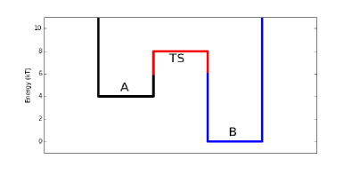
(b)

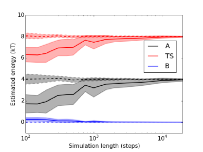
Figure 1: Comparison of WHAM and dTRAM estimation results using three independent trajectories sampling from three discrete states (two unbiased trajectories starting in $A$ and $B$ respectively, and biased trajectory sampling from a flat energy landscape over $A$, $TS$ and $B$). (a) Schematic of the energies of three states. Error bars correspond to one standard deviation of the estimate computed over 25 independent runs. (b) Estimation of the energies of $A$, $TS$ and $B$ using WHAM (solid lines) and dTRAM (dashed lines).

III.2 Umbrella sampling

In umbrella sampling, one introduces for each simulation $k$ an additive bias potential, such that our total potential in simulation $k$ is given by

$$u_{i}^{(k)}=u_{i}+b_{i}^{(k)}$$ (31)

where $i$ is a bin index of one or several finely discretized coordinates in which the bias potential is acting. $u_{i}$ is the unbiased potential evaluated at bin $i$ (usually at its center), and $b_{i}^{(k)}$ is the value of the $k$th umbrella (bias) potential. All energies are dimensionless (i.e. in units of the thermal energy $k_{B}T$). The biased equilibrium probabilities are proportional to:

$$\pi_{i}^{(k)} \propto \mathrm{e}^{-u_{i}^{(k)}}=\gamma_{i}^{(k)}\pi_{i}$$ (32)

with the unbiased equilibrium probability and the reweighting factors given by :

$$\pi_{i} = \frac{\mathrm{e}^{-u_{i}}}{\sum_{j}\mathrm{e}^{-u_{j}}}$$ (33)

$$\gamma_{i}^{(k)} = \mathrm{e}^{-b_{i}^{(k)}}$$ (34)

Umbrella sampling is typically employed using stiff constraining potentials, such that the simulations quickly decorrelate. In such a scenario, WHAM is a suitable estimator for extracting unbiased equilibrium probabilities and free energy differences. However, an analysis of umbrella sampling data can indeed benefit from using dTRAM. Firstly, dTRAM uses conditional transition events, and the number of statistically independent observations thus depends on a lag time $\tau$ which can be thought of as a local decorrelation time, i.e. a time at which transitions become statistically independent. This time is generally shorter than the global decorrelation time (or statistical inefficiency) $t_{corr}$, at which samples generated by the trajectory become statistically independent. Thus, whenever $t_{corr}$ is longer than the interval at which configurations are saved, dTRAM will be able to exploit that this data more efficiently than WHAM. This should lead to improved estimates.

Moreover, umbrella sampling can, in conjunction with WHAM, result in systematic errors that can be avoided with a TRAM estimator: As shown inRosta and Hummer (2014), using umbrellas that are too weak to stabilize the simulation at a transition state can lead to umbrella simulations that still have high internal free energy barriers and therefore do not generate samples that are drawn from the respective equilibrium distribution. Although a WHAM estimate would be correct in the limit of infinitely long simulation times, it may provide drastically biased estimates for practical simulation times.

Here, we employ umbrella sampling simulations on a one-dimensional double-well potential with a dimensionless energy:

$$u\left(x\right)=\frac{1}{4}x^{4}-5x^{2}-9.9874,$$ (35)

illustrated in Fig. 2B,C. The configuration space is discretized using a one dimensional binning: All $x$-values are assigned to the closest point from the set $\left\{-5,-4.9,\ldots,4.9,5\right\}$, generating up to 101 discrete states. However, in practice only about 80 states are visited and we exclude empty bins from the analysis. Umbrella sampling simulations are conducted using $K=11$ different biasing potentials given by:

$$b^{(k)}\left(x\right)=4\left(x-\bar{x}^{(k)}\right)^{2},\quad\text{for }k=1,\ldots,11$$ (36)

where $\bar{x}^{(k)}=k-6$ is the center of the $k$-th biasing potential. The dynamics are simulated using the Metropolis process described in Appendix C. The bias potentials are chosen relatively weak, such that the umbrella simulations near the transition state contain rare events . In this case, WHAM is a poor estimator because it takes relatively long to generate statistically independent samples.

In order to apply dTRAM, we evaluate all bias potentials for each discrete state, compute the reweighting factors according to Eq. (34), and store this information in a reweighting matrix. We additionally store all state-to-state transition counts $c_{ij}^{(k)}$ for each umbrella simulation $k$. Given this data the dTRAM estimation is computed by iterating equations (16-17) to convergence.

The performances of WHAM and dTRAM are compared in terms of the mean error of the estimated energy barriers:

$$\mathrm{error}=\frac{1}{2}\left(\left|\Delta u_{AB}-\Delta u_{AB}^{\mathrm{approx}}\right|+\left|\Delta u_{BA}-\Delta u_{BA}^{\mathrm{approx}}\right|\right)$$ (37)

where $\Delta u_{AB}$ and $\Delta u_{BA}$ are the energy barriers for the $A\rightarrow B$ and $B\rightarrow A$ process, respectively, and the superscript “$\mathrm{approx}$” represents the approximate value obtained from the estimated $u(x)$. Fig. 2A compares the energy barrier estimation error using WHAM (black) and dTRAM (red) as a function of the length of the umbrella simulations. In addition, estimation results our earlier approximate TRAM method from Wu and Noé (2014) are shown in blue. Fig. 2B and C show the energy profile estimated from the data using trajectory lengths of $910$ and $10000$ steps per umbrella, respectively. All means and standard deviations are obtained by repeating the simulation 30 times.

It is apparent that both estimators converge to the correct energy barriers and energy profile in the limit of a large amount of simulation data. For short simulations, the dTRAM estimates are significantly better than the WHAM and approximate TRAM estimates - or in other words much less simulation data is needed with dTRAM to obtain estimates of equal quality than when WHAM or approximate TRAM are used.

(A)

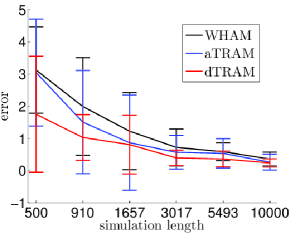
(B)

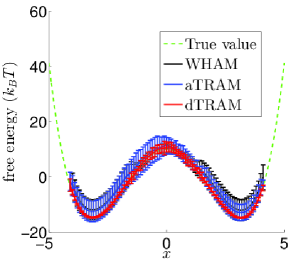
(C)

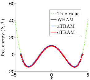
Figure 2: Estimation results of WHAM, the present method (dTRAM), and our early approximate TRAM method (aTRAM) from Wu and Noé (2014) based on umbrella sampling simulations in a double-well potential. (A) Mean and standard deviation of the energy barrier estimation error calculated over $30$ independent umbrella sampling runs with $K=11$ umbrellas each. The $x$-Axis shows the number of steps in an umbrella trajectory. (B) Mean and standard deviation of estimates of the potential $u(x)$ generated by WHAM, dTRAM and approximate TRAM using a trajectory length of $500$. (C) Same as (B), but with a trajectory length of $10000$.

In order to demonstrate the validity of dTRAM on molecular dynamics data of a large protein system, we have used it to analyze umbrella sampling simulations of the passage of Na⁺ ions through the transmembrane pore of the GLIC channel (Fig. 3). The data was generated in the simulations of Zhu and Hummer Zhu and Hummer (2012). WHAM and dTRAM provide a similar free energy profile (Fig. 3B), but for a given number of bins used to discretize the membrane normal used as a reaction coordinate, dTRAM provides a smaller systematic error. The systematic error is measured in terms of the energy difference calculated for the two end-states which should be 0 as a result of the periodic boundary conditions used in the simulation (Fig. 3C).

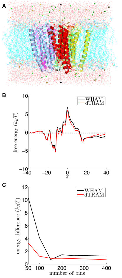
Figure 3: Estimation results of WHAM and dTRAM based on umbrella sampling simulations of Na⁺ passage through a GLIC channel using simulations of Zhu and Hummer Zhu and Hummer (2012). (A) Structure of the ion channel. (B) Free energy profile computed by WHAM and dTRAM when using 400 bins to discretize the reaction coordinate (membrane normal). (C) Systematic estimating error of the energies of the end-states, measured by its difference from 0, as a function of the number of discretization bins used.

IV Conclusions

We have derived a maximum likelihood estimator for the transition-based reweighting analysis method (TRAM). This estimator optimally combines simulation trajectories produced at different thermodynamic states. This is done by taking into account both the time correlations in the trajectories via transition counts, and by considering that the weight of every configuration can be given in any thermodynamic state via the Boltzmann distribution. The present estimator operates a configuration space discretization, and in particular also discretizes the reweighting factors between different thermodynamic states. Hence we call the present method discrete TRAM, or in short dTRAM.

dTRAM combines ideas from the weighted histogram analysis method (WHAM) and reversible Markov state models (MSMs). We have shown that dTRAM is in fact a proper generalization of both methods, i.e. both the WHAM estimator and the reversible MSM estimator can be derived as special cases from the dTRAM equations. Consequently, dTRAM can be applied to any kind of simulation data that either WHAM or MSMs can be applied to. In particular, dTRAM is useful for getting improved estimates from general-ensemble simulations (replica-exchange molecular dynamics, parallel or simulated tempering), multiple biased simulations (umbrella sampling, metadynamics, conformational flooding etc). Like MSMs, dTRAM is useful for obtaining estimates from swarms of short simulations that are not in global equilibrium, but beyond MSMs it can do so for trajectories produced under different thermodynamic conditions, such as temperatures or Hamiltonians.

dTRAM provides estimates for both the equilibrium distribution at a thermodynamic state of interest, and the kinetics at the thermodynamic states simulated at. The kinetic estimates should be treated with care as they are only useful when the data admits the choice of a lagtime that is sufficiently long to parametrize a Markov model that can predict long-term kinetics. For such estimates, it should be checked whether they are converged as a function of the lag time, as it is common practice in Markov state modeling. We will investigate the suitability of dTRAM to estimate kinetic data in future work. In the present paper we have only worked with short trajectory segments, and hence have only used dTRAM in order to estimate equilibrium distributions and free energies. It has been demonstrated that dTRAM provides superior estimates of these properties compared to WHAM when applied to biased simulations.

The present reweighting formulation is straightforwardly applied when the configuration space can be discretized in such a way that the bias factor $\gamma_{i}^{(k)}$ is approximately constant within each bin. Although such a discretization is easily done for umbrella sampling while biasing one or two coordinates, it is unsuitable in other cases, such as replica-exchange simulations. It has been suggested to construct a joint discretization in configuration and energy space Gallicchio et al. (2005). An optimal solution to the problem will involve a self-consistent evaluation of $\gamma_{i}^{(k)}$ in a way that integrates the sampled configurations assigned to bin $i$ with a MBAR-like approach Shirts and Chodera (2008).

A python implementation of the dTRAM method is available under https://github.com/markovmodel/pytram.

Acknowledgements

The authors thank following colleagues for enlightening discussions: John D. Chodera (MSKCC, New York), Gerhard Hummer (MPI for Biophysics, Frankfurt), Alessandro Laio (SISSA, Trieste), Roland R. Netz (FU Berlin) and the entire CMB team at FU Berlin. We thank Fangqiang Zhu for providing us with the umbrella sampling simulation data of the GLIC ion channel. This work was funded from following grants: WU 744/ 1-1 and DFG SFB 1114 (Wu), DFG SFB 740 and 958 (Mey), ERC grant “pcCell” (Noé).

Appendix A: Discrete TRAM: Derivation and proofs

A.1 Lagrange duality

A detailed description of Lagrange duality theory we refer to textbooks Hiriart-Urruty and Lemaréchal (1993a, b). Here we just summarize a few aspects of the theory relevant for solving the TRAM problem.

Consider a constrained minimization problem of the following form:

$$\begin{array}[]{cl}\min_{\mathbf{x}}&f\left(\mathbf{x}\right)\\ s.t.&f_{e}\left(\mathbf{x}\right)=0\end{array}$$ (38)

The Lagrangian function can be defined by

$$\Lambda\left(\mathbf{x},\mathbf{v}\right)=f\left(\mathbf{x}\right)+\mathbf{v}^{\intercal}f_{e}\left(\mathbf{x}\right)$$ (39)

If (38) is a convex problem and some technical assumption such as Slater condition holds, it can be proven that (38) is equivalent to the following maximization problem:

$$\max_{\mathbf{v}}g(\mathbf{v})$$ (40)

where $g(\mathbf{v})$ is the Lagrange dual function defined by

$$g(\mathbf{v}):=\min_{\mathbf{x}}\Lambda\left(\mathbf{x},\mathbf{v}\right)$$ (41)

The equivalence here means the optimal values of the two problems are equal, i.e., the solution $\mathbf{x}^{*}$ to (38) and the solution $\mathbf{v}^{*}$ to (40) satisfies $g\left(\mathbf{v}^{*}\right)=f\left(\mathbf{x}^{*}\right)$. Moreover,

$$\mathbf{x}^{*}=\arg\min_{\mathbf{x}}\Lambda\left(\mathbf{x},\mathbf{v}^{*}\right)$$ (42)

A.2 Single thermodynamic state

We first consider the dual Lagrange approach to solving dTRAM at a single thermodynamic state, i.e. the situation that is equivalent with a reversible Markov state model. Here we first ignore the normalization of the stationary distribution $\boldsymbol{\pi}$, i.e., $\sum_{i}\pi_{i}$ may not be equal to $1$. The maximum likelihood estimation of the transition matrix $\mathbf{P}$ with a fixed equilibrium distribution $\boldsymbol{\pi}$ is given by the following optimization problem:

$$\begin{array}[]{cl}\min_{\mathbf{P}}&-L\left(\mathbf{P}\mid\mathbf{C}\right)\\ s.t.&\pi_{i}p_{ij}=\pi_{j}p_{ji}\\ &\sum_{j}p_{ij}=1\end{array}$$ (43)

where

$$L\left(\mathbf{P}\mid\mathbf{C}\right)=\sum_{i,j}c_{ij}\ln p_{ij}$$ (44)

is the log-likelihood function of $\mathbf{P}$. By using the Lagrange duality theory, we have the following lemma:

Lemma: The minimization problem (43) is equivalent to the maximization problem

$$\begin{array}[]{crl}\min_{\mathbf{v}}&h_{\mathbf{C}}\left(\boldsymbol{\pi},\mathbf{v}\right)=&\sum_{i,j}c_{ij}\ln\left(\pi_{i}v_{j}+\pi_{j}v_{i}\right)\\ &&-\sum_{i,j}c_{ij}\ln\pi_{j}-\sum_{i}v_{i}\\ &&-\sum_{i,j}c_{ij}\ln\left(c_{ij}+c_{ji}\right)+\sum_{i,j}c_{ij}\end{array}$$ (45)

and the optimal solution $\mathbf{P}^{*}$ to (43) and the optimal solution $\mathbf{v}^{*}$ to (45) satisfy

$$p_{ij}^{*}=\frac{\left(c_{ij}+c_{ji}\right)\pi_{j}}{\pi_{i}v_{j}^{*}+\pi_{j}v_{i}^{*}}$$ (46)

Proof: The Lagrangian function of (43) is defined as

$$\Lambda_{\boldsymbol{\pi}}\left(\mathbf{P},\boldsymbol{\lambda},\mathbf{v}\right) = -\sum_{i,j}c_{ij}\ln p_{ij}+\sum_{i,j}\lambda_{ij}\left(\pi_{i}p_{ij}-\pi_{j}p_{ji}\right)$$ (47)

$$+\sum_{i}v_{i}\left(\sum_{j}p_{ij}-1\right)$$

$$= -\sum_{i,j}c_{ij}\ln p_{ij}+\sum_{i,j}\left(\pi_{i}\left(\lambda_{ij}-\lambda_{ji}\right)+v_{i}\right)p_{ij}$$

$$-\sum_{i}v_{i}.$$

Note that

$$\frac{\partial\Lambda_{\boldsymbol{\pi}}}{\partial p_{ij}}=-\frac{c_{ij}}{p_{ij}}+\pi_{i}\left(\lambda_{ij}-\lambda_{ji}\right)+v_{i}$$ (48)

Then the dual function of (43) is

$$g_{\boldsymbol{\pi}}\left(\lambda,\nu\right) = \min_{\mathbf{P}}\Lambda_{\boldsymbol{\pi}}\left(\mathbf{P},\boldsymbol{\lambda},\mathbf{v}\right)$$ (49)

$$= \Lambda\left(\left[\frac{c_{ij}}{\pi_{i}\left(\lambda_{ij}-\lambda_{ji}\right)+v_{i}}\right],\boldsymbol{\lambda},\mathbf{v}\right)$$

$$= -\sum_{i,j}c_{ij}\ln\left(\frac{c_{ij}}{\pi_{i}\left(\lambda_{ij}-\lambda_{ji}\right)+v_{i}}\right)$$

$$+\sum_{i,j}c_{ij}-\sum_{i}v_{i}$$

$$= \sum_{i,j}c_{ij}\ln\left(\pi_{i}\left(\lambda_{ij}-\lambda_{ji}\right)+v_{i}\right)-\sum_{i}v_{i}$$

$$-\sum_{i,j}c_{ij}\ln c_{ij}+\sum_{i,j}c_{ij}$$

and (43) is equivalent to the maximization problem

$$\max_{\boldsymbol{\lambda},\mathbf{v}}g_{\boldsymbol{\pi}}\left(\boldsymbol{\lambda},\mathbf{v}\right)$$ (50)

From (49), we can get

$$\frac{\partial g_{\boldsymbol{\pi}}\left(\boldsymbol{\lambda},\mathbf{v}\right)}{\partial\lambda_{ij}}=\frac{c_{ij}\pi_{i}}{\pi_{i}\left(\lambda_{ij}-\lambda_{ji}\right)+v_{i}}-\frac{c_{ji}\pi_{j}}{\pi_{j}\left(\lambda_{ji}-\lambda_{ij}\right)+v_{j}}$$ (51)

and

$$\frac{\partial g_{\boldsymbol{\pi}}\left(\boldsymbol{\lambda},\mathbf{v}\right)}{\partial\lambda_{ij}}=0\Leftrightarrow\lambda_{ij}-\lambda_{ji}=\frac{c_{ij}\pi_{i}v_{j}-c_{ji}\pi_{j}v_{i}}{\left(c_{ij}+c_{ji}\right)\pi_{i}\pi_{j}}$$ (52)

Therefore,

$$\max_{\boldsymbol{\lambda}}g_{\boldsymbol{\pi}}\left(\boldsymbol{\lambda},\mathbf{v}\right) = \sum_{i,j}c_{ij}\ln\left(\pi_{i}\frac{c_{ij}\pi_{i}v_{j}-c_{ji}\pi_{j}v_{i}}{\left(c_{ij}+c_{ji}\right)\pi_{i}\pi_{j}}+v_{i}\right)$$ (53)

$$-\sum_{i}v_{i}-\sum_{i,j}c_{ij}\ln c_{ij}+\sum_{i,j}c_{ij}$$

$$= \sum_{i,j}c_{ij}\ln\left(\frac{c_{ij}\left(\pi_{i}v_{j}+\pi_{j}v_{i}\right)}{\left(c_{ij}+c_{ji}\right)\pi_{j}}\right)$$

$$-\sum_{i}v_{i}-\sum_{i,j}c_{ij}\ln c_{ij}+\sum_{i,j}c_{ij}$$

$$= \sum_{i,j}c_{ij}\ln\left(\pi_{i}v_{j}+\pi_{j}v_{i}\right)-\sum_{i,j}c_{ij}\ln\pi_{j}$$

$$-\sum_{i}v_{i}-\sum_{i,j}c_{ij}\ln\left(c_{ij}+c_{ji}\right)+\sum_{i,j}c_{ij}$$

$$= h_{\mathbf{C}}\left(\boldsymbol{\pi},\mathbf{v}\right)$$

and the optimal value of (43) is equal to

$$\max_{\boldsymbol{\lambda},\mathbf{v}}g_{\boldsymbol{\pi}}\left(\boldsymbol{\lambda},\mathbf{v}\right)=\max_{\mathbf{v}}\left(\max_{\boldsymbol{\lambda}}g_{\boldsymbol{\pi}}\left(\boldsymbol{\lambda},\mathbf{v}\right)\right)=\max_{\mathbf{v}}h_{\mathbf{C}}\left(\boldsymbol{\pi},\mathbf{v}\right)$$ (54)

and

$$p_{ij}^{*} = \frac{c_{ij}}{\pi_{i}\left(\lambda_{ij}^{*}-\lambda_{ji}^{*}\right)+v_{i}^{*}}$$ (55)

$$= \frac{c_{ij}}{\pi_{i}\frac{c_{ij}\pi_{i}v_{j}^{*}-c_{ji}\pi_{j}v_{i}^{*}}{\left(c_{ij}+c_{ji}\right)\pi_{i}\pi_{j}}+v_{i}^{*}}$$

$$= \frac{\left(c_{ij}+c_{ji}\right)\pi_{j}}{\pi_{i}v_{j}^{*}+\pi_{j}v_{i}^{*}}$$

where

$$\lambda_{ij}^{*}-\lambda_{ji}^{*}=\frac{c_{ij}\pi_{i}v_{j}^{*}-c_{ji}\pi_{j}v_{i}^{*}}{\left(c_{ij}+c_{ji}\right)\pi_{i}\pi_{j}}$$ (56)

We now consider the case that the stationary distribution is unknown. In this case, the maximum likelihood estimate of $\pi$ is

$$\boldsymbol{\pi}^{*} = \arg\min_{\boldsymbol{\pi}}\left(\min_{\mathbf{P}\text{ is feasible to \eqref{eq:single-1}}}-L\left(\mathbf{P}\right)\right)$$ (57)

$$= \arg\min_{\boldsymbol{\pi}}\left(\max_{\mathbf{v}}h_{\mathbf{C}}\left(\boldsymbol{\pi},\mathbf{v}\right)\right)$$

A.3 Multiple Simulations

If we further consider multiple biased simulations with $\pi_{i}^{(k)}\propto\gamma_{i}^{(k)}\pi_{i}$, we can also conclude that the maximum likelihood estimate of $\boldsymbol{\pi}$ can be given by the following min-max problem:

$$\min_{\boldsymbol{\pi}}\max_{\mathbf{v}^{(1)},\ldots,\mathbf{v}^{(K)}}\sum_{k}h_{\mathbf{C}^{(k)}}\left(\mathrm{diag}\left(\boldsymbol{\gamma}^{(k)}\right)\boldsymbol{\pi},\mathbf{v}^{(k)}\right)$$ (58)

For the sake of convenience, here we define $u_{i}=-\ln\pi_{i}$. Then (58) can be rewritten as

$$\min_{\mathbf{u}}\max_{\mathbf{v}^{(1)},\ldots,\mathbf{v}^{(K)}}\sum_{k}h_{\mathbf{C}^{(k)}}\left(\mathrm{diag}\left(\boldsymbol{\gamma}^{(k)}\right)\exp\left(-\mathbf{u}\right),\mathbf{v}^{(k)}\right)$$ (59)

Because $h\left(\exp\left(-\mathbf{u}\right),\mathbf{v}\right)$ is a concave function of $\mathbf{v}$ if $\mathbf{u}$ is fixed and a convex function of $\mathbf{u}$ if $\mathbf{v}$ is fixed, the solution to (59) is a saddle point and characterized by (see Section 10.3.4 in Boyd and Vandenberghe (2004))

$$\frac{\partial h_{\mathbf{C}^{(k)}}\left(\mathrm{diag}\left(\boldsymbol{\gamma}^{(k)}\right)\exp\left(-\mathbf{u}\right),\mathbf{v}^{(k)}\right)}{\partial\nu_{i}^{(k)}} = 0,$$

$$\quad\quad\quad\quad i=1,\ldots,n,\>k=1,\ldots,K$$ (60)

$$\frac{\partial\sum_{k}h_{\mathbf{C}^{(k)}}\left(\mathrm{diag}\left(\boldsymbol{\gamma}^{(k)}\right)\exp\left(-\mathbf{u}\right),\mathbf{v}^{(k)}\right)}{\partial u_{i}} = 0,$$

$$\quad\quad\quad\quad i=1,\ldots,n$$ (61)

Considering that

$$\frac{\partial h_{\mathbf{C}}\left(\mathrm{diag}\left(\boldsymbol{\gamma}\right)\exp\left(-\mathbf{u}\right),\mathbf{v}\right)}{\partial v_{i}}=\sum_{j}\frac{\left(c_{ij}+c_{ji}\right)\gamma_{j}\pi_{j}}{\gamma_{i}\pi_{i}v_{j}+\gamma_{j}\pi_{j}v_{i}}-1$$ (62)

and

$$\frac{\partial h_{\mathbf{C}}\left(\mathrm{diag}\left(\boldsymbol{\gamma}\right)\exp\left(-\mathbf{u}\right),\mathbf{v}\right)}{\partial u_{i}}$$

$$= \frac{\partial h_{\mathbf{C}}\left(\mathrm{diag}\left(\boldsymbol{\gamma}\right)\boldsymbol{\pi},\mathbf{v}\right)}{\partial\pi_{i}}\frac{\partial\pi_{i}}{\partial u_{i}}$$

$$= -\pi_{i}\left(\sum_{j}\frac{\left(c_{ij}+c_{ji}\right)\gamma_{i}v_{j}}{\gamma_{i}\pi_{i}v_{j}+\gamma_{j}\pi_{j}v_{i}}-\frac{\sum_{j}c_{ji}}{\pi_{i}}\right)$$

$$= \sum_{j}c_{ji}-\sum_{j}\frac{\left(c_{ij}+c_{ji}\right)\gamma_{i}\pi_{i}v_{j}}{\gamma_{i}\pi_{i}v_{j}+\gamma_{j}\pi_{j}v_{i}}$$ (64)

We can conclude that the optimal solution to (58) should satisfy

$$\sum_{j}\frac{\left(c_{ij}^{(k)}+c_{ji}^{(k)}\right)\gamma_{j}^{(k)}\pi_{j}}{\gamma_{i}^{(k)}\pi_{i}v_{j}^{(k)}+\gamma_{j}^{(k)}\pi_{j}v_{i}^{(k)}} = 1$$ (65)

$$\pi_{i}\sum_{j,k}\frac{\left(c_{ij}^{(k)}+c_{ji}^{(k)}\right)\gamma_{i}^{(k)}v_{j}^{(k)}}{\gamma_{i}^{(k)}\pi_{i}v_{j}^{(k)}+\gamma_{j}^{(k)}\pi_{j}v_{i}^{(k)}} = \sum_{j,k}c_{ji}^{(k)}$$ (66)

This leads to the following iterative algorithm for unbiased estimation of multiple simulations:

$$v_{i}^{(k),\mathrm{new}} = v_{i}^{(k)}\sum_{j}\frac{\left(c_{ij}^{(k)}+c_{ji}^{(k)}\right)\gamma_{j}^{(k)}\pi_{j}}{\left(\gamma_{i}^{(k)}\pi_{i}v_{j}^{(k)}+\gamma_{j}^{(k)}\pi_{j}v_{i}^{(k)}\right)},$$ (67)

$$\quad\quad\quad\quad\quad\quad\quad\quad\quad\quad\quad\text{for }i=1,\ldots n$$

$$\pi_{i}^{\mathrm{new}} = \frac{\sum_{k,j}c_{ji}^{(k)}}{\sum_{k,j}\frac{\left(c_{ij}^{(k)}+c_{ji}^{(k)}\right)\gamma_{i}^{(k)}v_{j}^{(k)}}{\left(\gamma_{i}^{(k)}\pi_{i}v_{j}^{(k)}+\gamma_{j}^{(k)}\pi_{j}v_{i}^{(k)}\right)}},$$ (68)

$$\quad\quad\quad\quad\quad\quad\quad\quad\quad\quad\quad\text{for }i=1,\ldots n$$

A.4 Asymptotic correctness of dTRAM

Here we show that dTRAM converges to the correct equilibrium distribution and transition probabilities in the limit of large statistics. In this limit, either achieved through long simulation trajectories or many short simulation trajectories, the count matrices $\mathbf{C}^{(k)}=[c_{ij}^{(k)}]$ become:

$$c_{ij}^{(k)}=N_{i}^{(k)}\bar{p}_{ij}^{(k)}$$ (69)

where $\bar{\mathbf{P}}^{(k)}=[\bar{p}_{ij}^{(k)}]$ is the matrix of exact transition probabilities (no statistical error), which satisfies

$$\bar{\pi}_{i}\gamma_{i}^{(k)}\bar{p}_{ij}^{(k)}=\bar{\pi}_{j}\gamma_{j}^{(k)}\bar{p}_{ji}^{(k)}$$ (70)

where $\boldsymbol{\pi}=[\bar{\pi}_{i}]$ are the exact stationary probabilities of configuration states. Inserting (69) into the dTRAM equations (12-13), we obtain:

$$\sum_{k}\sum_{j}\frac{\left(c_{ij}^{(k)}+c_{ji}^{(k)}\right)\gamma_{i}^{(k)}\bar{\pi}_{i}N_{j}^{(k)}}{\gamma_{i}^{(k)}\bar{\pi}_{i}N_{j}^{(k)}+\gamma_{j}^{(k)}\bar{\pi}_{j}N_{i}^{(k)}}$$ (71)

$$= \sum_{k}\sum_{j}\frac{\left(N_{i}^{(k)}\bar{p}_{ij}^{(k)}+N_{j}^{(k)}\bar{p}_{ji}^{(k)}\right)\gamma_{i}^{(k)}\bar{\pi}_{i}N_{j}^{(k)}}{\gamma_{i}^{(k)}\bar{\pi}_{i}N_{j}^{(k)}+\gamma_{j}^{(k)}\bar{\pi}_{j}N_{i}^{(k)}}$$ (72)

$$= \sum_{k}\sum_{j}\frac{\left(N_{i}^{(k)}\gamma_{j}^{(k)}\bar{\pi}_{j}+N_{j}^{(k)}\gamma_{i}^{(k)}\bar{\pi}_{i}\right)\bar{p}_{ji}^{(k)}N_{j}^{(k)}}{\gamma_{i}^{(k)}\bar{\pi}_{i}N_{j}^{(k)}+\gamma_{j}^{(k)}\bar{\pi}_{j}N_{i}^{(k)}}$$ (73)

$$= \sum_{k}\sum_{j}\bar{p}_{ji}^{(k)}N_{j}^{(k)}$$ (74)

$$= \sum_{k}\sum_{j}c_{ji}^{(k)}$$ (75)

and thus the first dTRAM equation is satisfied. Furthermore, we obtain:

$$\sum_{j}\frac{\left(c_{ij}^{(k)}+c_{ji}^{(k)}\right)\gamma_{j}^{(k)}\bar{\pi_{j}}}{\gamma_{i}^{(k)}\bar{\pi}_{i}N_{j}^{(k)}+\gamma_{j}^{(k)}\bar{\pi}_{j}N_{i}^{(k)}}$$ (76)

$$= \sum_{j}\frac{\left(N_{i}^{(k)}\bar{p}_{ij}^{(k)}+N_{j}^{(k)}\bar{p}_{ji}^{(k)}\right)\gamma_{j}^{(k)}\bar{\pi_{j}}}{\gamma_{i}^{(k)}\bar{\pi}_{i}N_{j}^{(k)}+\gamma_{j}^{(k)}\bar{\pi}_{j}N_{i}^{(k)}}$$ (77)

$$= \sum_{j}\frac{N_{i}^{(k)}\bar{p}_{ij}^{(k)}\gamma_{j}^{(k)}\bar{\pi_{j}}+N_{j}^{(k)}\bar{p}_{ij}^{(k)}\gamma_{i}^{(k)}\bar{\pi_{i}}}{\gamma_{i}^{(k)}\bar{\pi}_{i}N_{j}^{(k)}+\gamma_{j}^{(k)}\bar{\pi}_{j}N_{i}^{(k)}}$$ (78)

$$= \sum_{j}\bar{p}_{ij}^{(k)}$$ (79)

$$= 1$$ (80)

and thus the second dTRAM equation is satisfied as well. From the above two equations, we can conclude that in the statistical limit (either achieved by long trajectories or many short trajectories), the solution of the dTRAM equations converges to the correct equilibrium distribution and the correct transition probabilities. Note that we have assumed that all trajectory data is in local equilibrium within each starting state $i$ - if this is not the case the counts $c_{ij}$ and thus also the estimated $\pi_{i}$ and $p_{ij}$ will be biased. Thus, if the data is of such a nature that local equilibrium is a concern (e.g. metadynamics or uncoupled short MD trajectories), all estimates should be computed as a function of the lag time $\tau$.

Appendix B: Double-well simulation model

The simulation trajectory $\{x_{t}^{(k)}\}_{t=0}^{M}$ is generated by a Metropolis simulation model, which is a reversible Markov chain with initial state $x_{0}^{(k)}=\bar{x}^{(k)}$, stationary distribution $\pi_{i}^{(k)}\propto\mathrm{e}^{-u_{i}-b_{i}^{(k)}}$, and transition probability

$$\Pr\left(x_{t+1}^{(k)}=x^{\prime}|x_{t}^{(k)}=x\right)$$ (81)

$$=\left\{\begin{array}[]{ll}\min\left\{\frac{\exp\left(-u\left(x^{\prime}\right)-v^{(k)}\left(x^{\prime}\right)\right)}{\exp\left(-u\left(x\right)-v^{(k)}\left(x\right)\right)}q\left(x|x^{\prime}\right),q\left(x^{\prime}|x\right)\right\},&x^{\prime}\neq x\\ 1-\sum_{y\neq x}\Pr\left(x_{t+1}^{(k)}=y|x_{t}^{(k)}=x\right),&x^{\prime}=x\end{array}\right.$$ (84)

where $q\left(x^{\prime}|x\right)$ denotes the proposal distribution which satisfies $q\left(x^{\prime}|x\right)\propto 1_{\left|x^{\prime}-x\right|\leq 0.2}$ and $\sum_{x^{\prime}}q\left(x^{\prime}|x\right)=1$.

References

- Greyer (1991) C. G. Greyer (American Statistical Association, New York, 1991) pp. 156–163.
- Hukushimi and Nemoto (1996) K. Hukushimi and K. Nemoto, J. Phys. Soc. Jpn. 65, 1604 (1996).
- Hansmann (1997) U. H. Hansmann, Chem. Phys. Let. 281, 140 (1997).
- Sugita and Okamato (1999) Y. Sugita and Y. Okamato, Chem. Phys. Lett. 314, 141 (1999).
- Marinari and Parisi (1992) E. Marinari and G. Parisi, Euro. Phys. Let. 19, 451 (1992).
- Torrie and Valleau (1977) G. M. Torrie and J. P. Valleau, J. Comp. Phys. 23, 187 (1977).
- Ferrenberg and Swendsen (1989) A. M. Ferrenberg and R. H. Swendsen, Phys. Rev. Lett. 63, 1195 (1989).
- Kumar et al. (1992) S. Kumar, D. Bouzida, R. H. Swendsen, P. A. Kollman, and J. M. Rosenberg, J. Comput. Chem. 13, 1011 (1992).
- Souaille and Roux (2001) M. Souaille and B. Roux, Comput. Phys. Commun. 135, 40 (2001).
- Shirts and Chodera (2008) M. R. Shirts and J. D. Chodera, J. Chem. Phys. 129, 124105 (2008).
- Sriraman et al. (2005) S. Sriraman, I. G. Kevrekidis, and G. Hummer, J. Phys. Chem. B 109, 6479 (2005).
- Minh and Chodera (2009) D. D. L. Minh and J. D. Chodera, J. Chem. Phys. 131, 134110 (2009).
- Chodera et al. (2011) J. D. Chodera, W. C. Swope, F. Noé, J.-H. Prinz, and V. S. Pande, J. Phys. Chem. 134, 244107 (2011).
- Prinz et al. (2011a) J.-H. Prinz, J. D. Chodera, V. S. Pande, W. C. Swope, J. C. Smith, and F. Noé, J. Chem. Phys. 134, 244108 (2011a).
- Du and Bolhuis (2013) W. Du and P. G. Bolhuis, J. Chem. Phys. 139, 044105 (2013).
- Bartels and Karplus (1997) C. Bartels and M. Karplus, J. Comp. Chem. 18, 1450 (1997).
- Sakuraba and Kitao (2009) S. Sakuraba and A. Kitao, Journal of computational chemistry 30, 1850 (2009).
- Wu and Noé (2014) H. Wu and F. Noé, SIAM Multiscale Model. Simul. 12, 25 (2014).
- Mey et al. (2014) A. S. J. S. Mey, H. Wu, and F. Noé, Phys. Rev. X 4, 041018 (2014).
- Rosta and Hummer (2014) E. Rosta and G. Hummer, J. Chem. Theo. Comput. (submitted) (2014).
- Shirts and Pande (2000) M. Shirts and V. S. Pande, Science 290, 1903 (2000).
- Noé et al. (2009) F. Noé, C. Schütte, E. Vanden-Eijnden, L. Reich, and T. Weikl, Proc. Natl. Acad. Sci. USA 106, 19011 (2009).
- Buch et al. (2011) I. Buch, T. Giorgino, and G. de Fabritiis, Proc. Natl. Acad. Sci. USA 108, 10184 (2011).
- Laio and Parrinello (2002) A. Laio and M. Parrinello, Proc. Natl. Acad. Sci. USA 99, 12562 (2002).
- Grubmüller (1995) H. Grubmüller, Phys. Rev. E 52, 2893 (1995).
- Schütte et al. (1999) C. Schütte, A. Fischer, W. Huisinga, and P. Deuflhard, J. Comput. Phys. 151, 146 (1999).
- Swope et al. (2004) W. C. Swope, J. W. Pitera, and F. Suits, The Journal of Physical Chemistry B 108, 6571 (2004).
- Singhal and Pande (2005) N. Singhal and V. S. Pande, J. Chem. Phys. 123, 204909 (2005).
- Noé et al. (2007) F. Noé, I. Horenko, C. Schütte, and J. C. Smith, J. Chem. Phys. 126, 155102 (2007).
- Chodera et al. (2007) J. D. Chodera, K. A. Dill, N. Singhal, V. S. Pande, W. C. Swope, and J. W. Pitera, J. Chem. Phys. 126, 155101 (2007).
- Buchete and Hummer (2008) N. V. Buchete and G. Hummer, J. Phys. Chem. B 112, 6057 (2008).
- Prinz et al. (2011b) J.-H. Prinz, H. Wu, M. Sarich, B. Keller, M. Senne, M. Held, J. D. Chodera, C. Schütte, and F. Noé, J. Chem. Phys. 134, 174105 (2011b).
- Sarich et al. (2010) M. Sarich, F. Noé, and C. Schütte, SIAM Multiscale Model. Simul. 8, 1154 (2010).
- Tan (2008) Z. Tan, J. Stat. Plan. Inf. 138, 1967 (2008).
- Tan et al. (2012) Z. Tan, E. Gallicchio, M. Lapelosa, and R. M. Levy, J. Chem. Phys. 136, 144102 (2012).
- Zhu and Hummer (2012) F. Zhu and G. Hummer, J. Comput. Chem. 33, 453 (2012).
- Noé (2008) F. Noé, J. Chem. Phys. 128, 244103 (2008).
- Bowman et al. (2009) G. R. Bowman, K. A. Beauchamp, G. Boxer, and V. S. Pande, J. Chem. Phys. 131, 124101+ (2009).
- Norris (1998) J. R. Norris, Markov Chains, Cambridge Series in Statistical and Probabilistic Mathematics, Vol. 4 (Cambridge University Press, Cambridge, 1998).
- Gallicchio et al. (2005) E. Gallicchio, M. Andrec, A. K. Felts, and R. M. Levy, J. Phys. Chem. B 109, 6722 (2005).
- Hiriart-Urruty and Lemaréchal (1993a) J.-B. Hiriart-Urruty and C. Lemaréchal, Convex Analysis and Minimization Algorithms I: Fundamentals (Springer, Heidelberg, 1993).
- Hiriart-Urruty and Lemaréchal (1993b) J.-B. Hiriart-Urruty and C. Lemaréchal, Convex Analysis and Minimization Algorithms II: Advanced theory and bundle methods (Springer, Heidelberg, 1993).
- Boyd and Vandenberghe (2004) S. Boyd and L. Vandenberghe, Convex Optimization (Cambridge University Press, 2004).